Monitoring Inter- and Intra-Seasonal Dynamics of Rapidly Degrading Ice-Rich Permafrost Riverbanks in the Lena Delta with TerraSAR-X Time Series

 , , ,
, , , 
Abstract
:1. Introduction
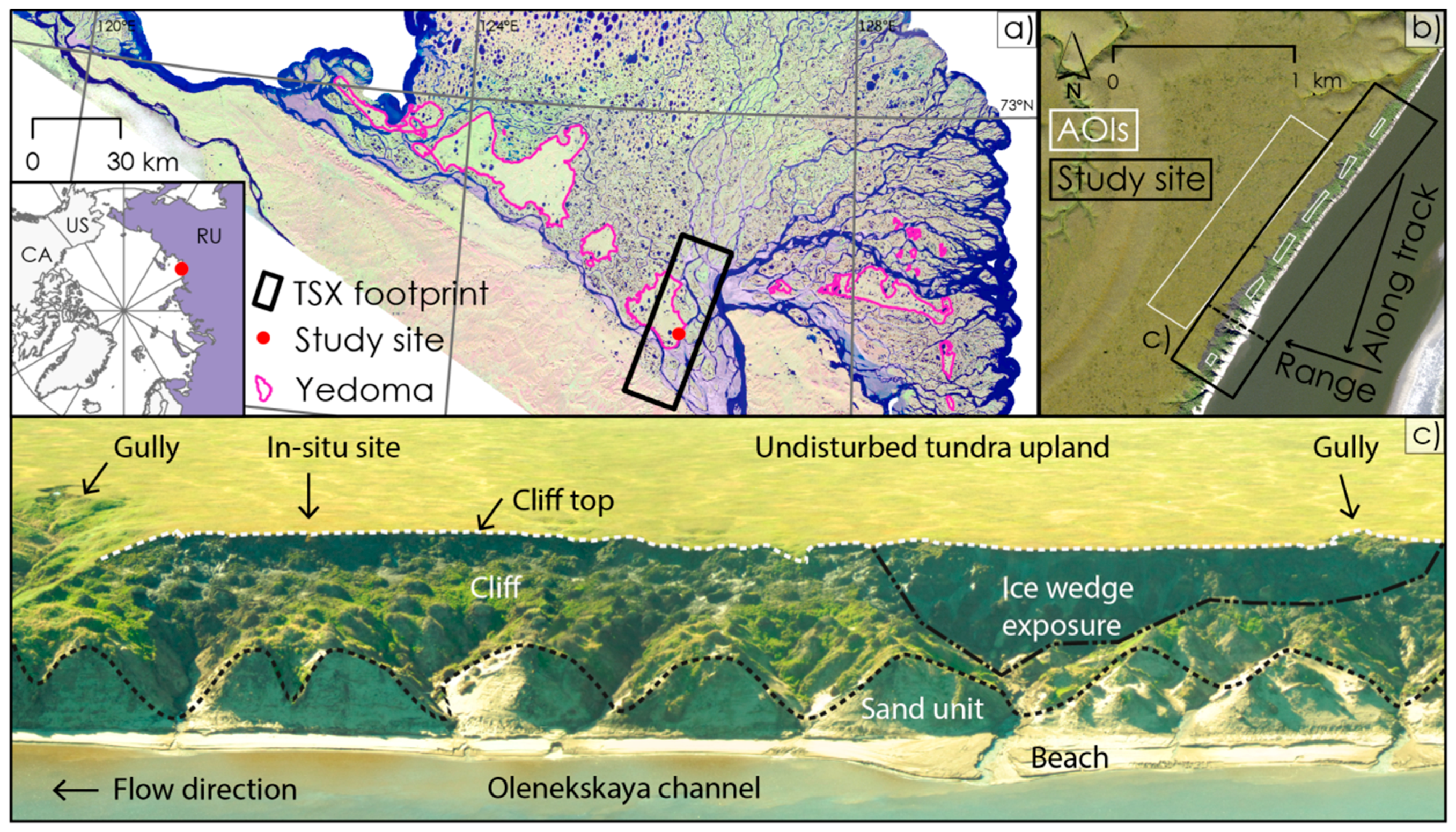
2. Study Area
3. Data and Methods
3.1. SAR Data and Processing
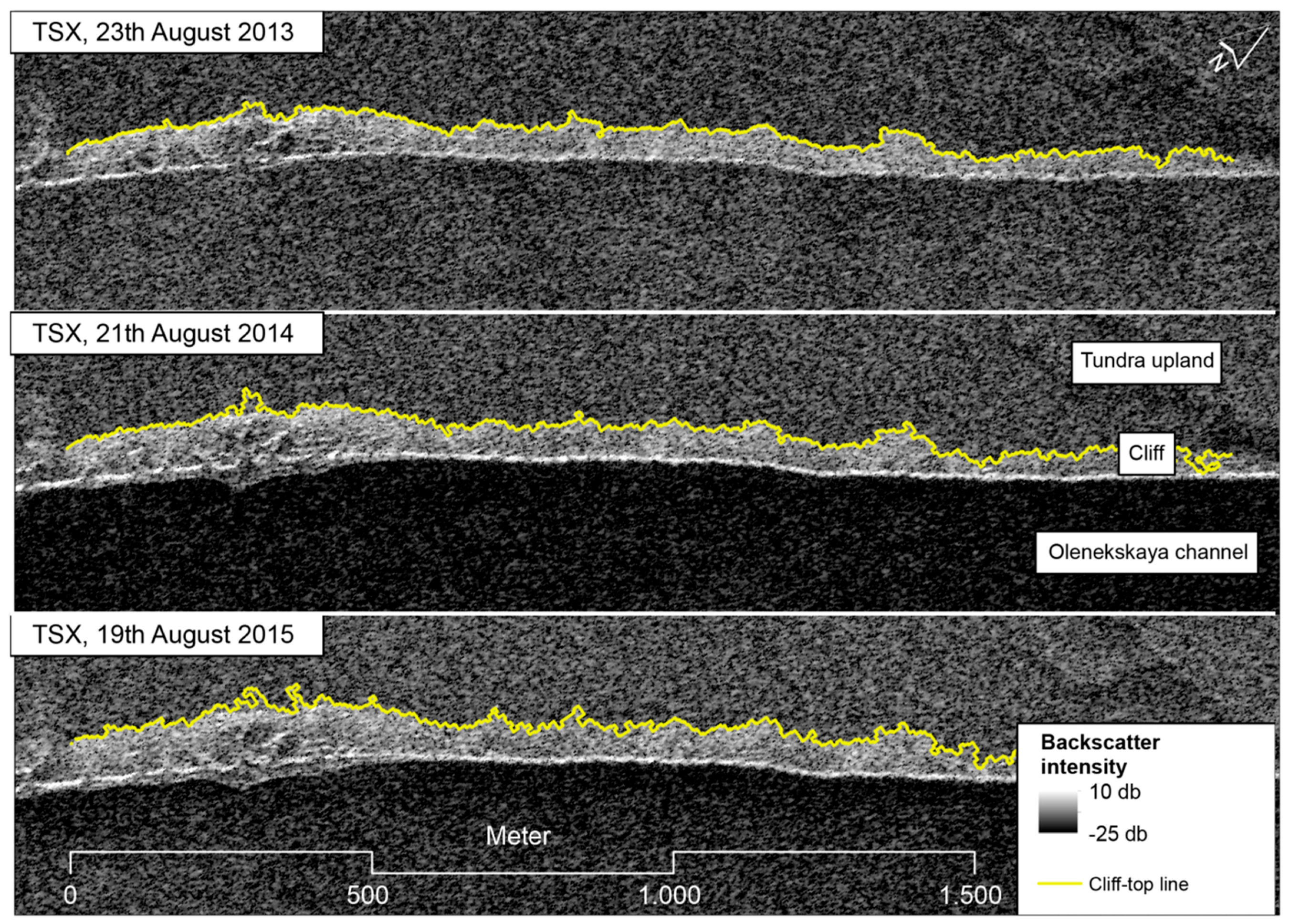
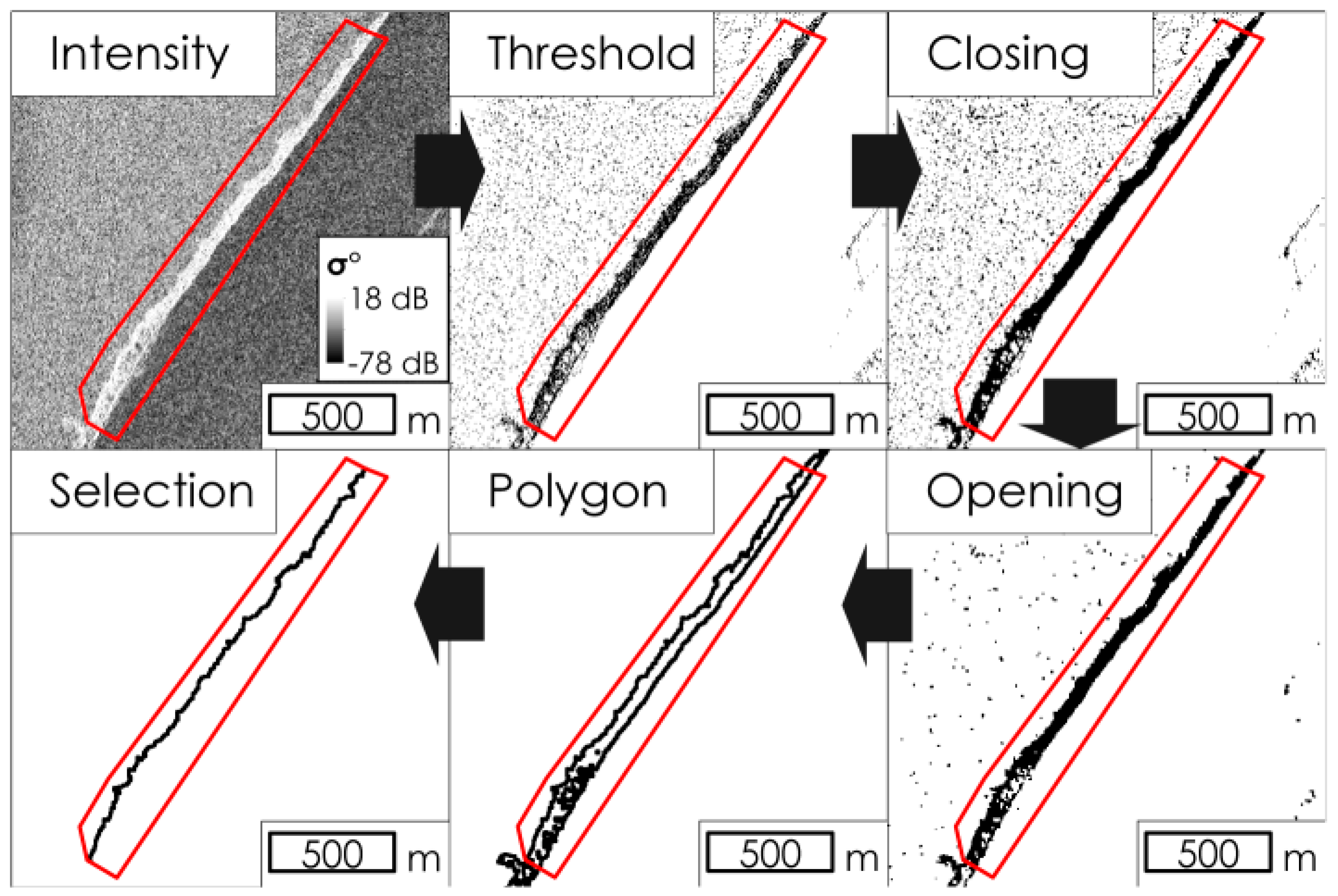
3.2. Automated Cliff-Top Line Extraction from SAR Data
3.3. Quantification of Cliff-Top Erosion with the Digital Shoreline Analysis System (DSAS)
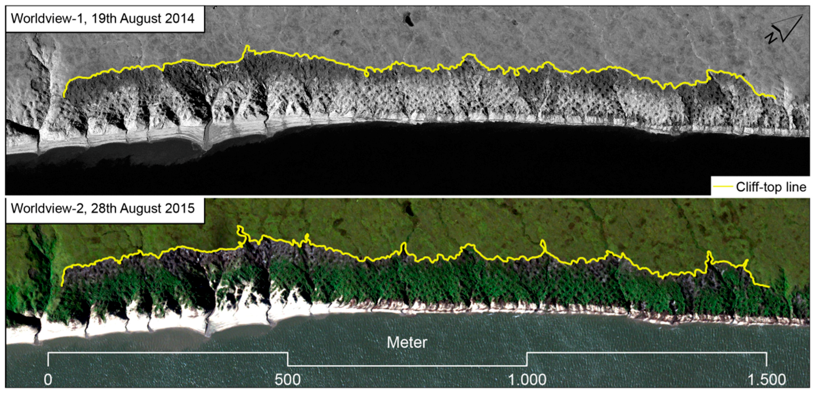
3.4. Cliff Top Mapping from Optical Satellite Data
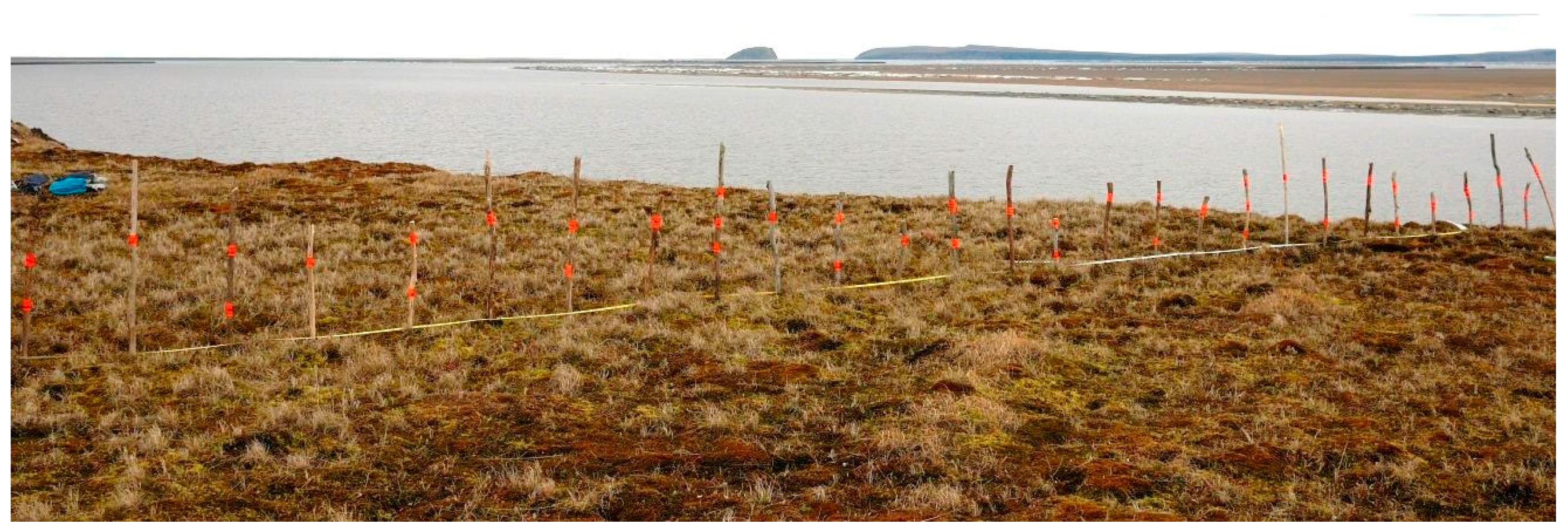
3.5. In-Situ Observations of Cliff-Top Erosion
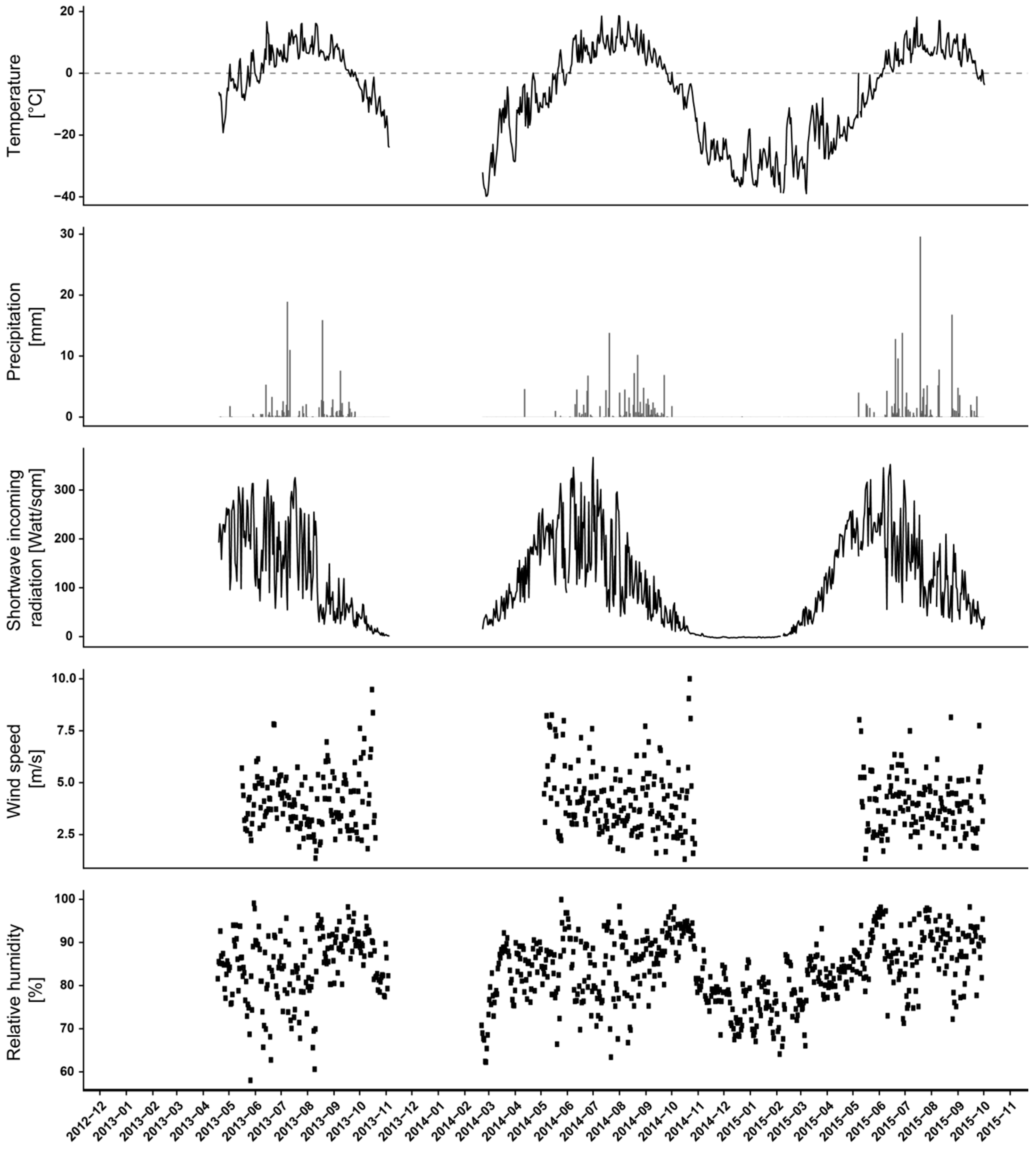
3.6. Climate Data
3.7. Statistical Data Analysis
4. Results
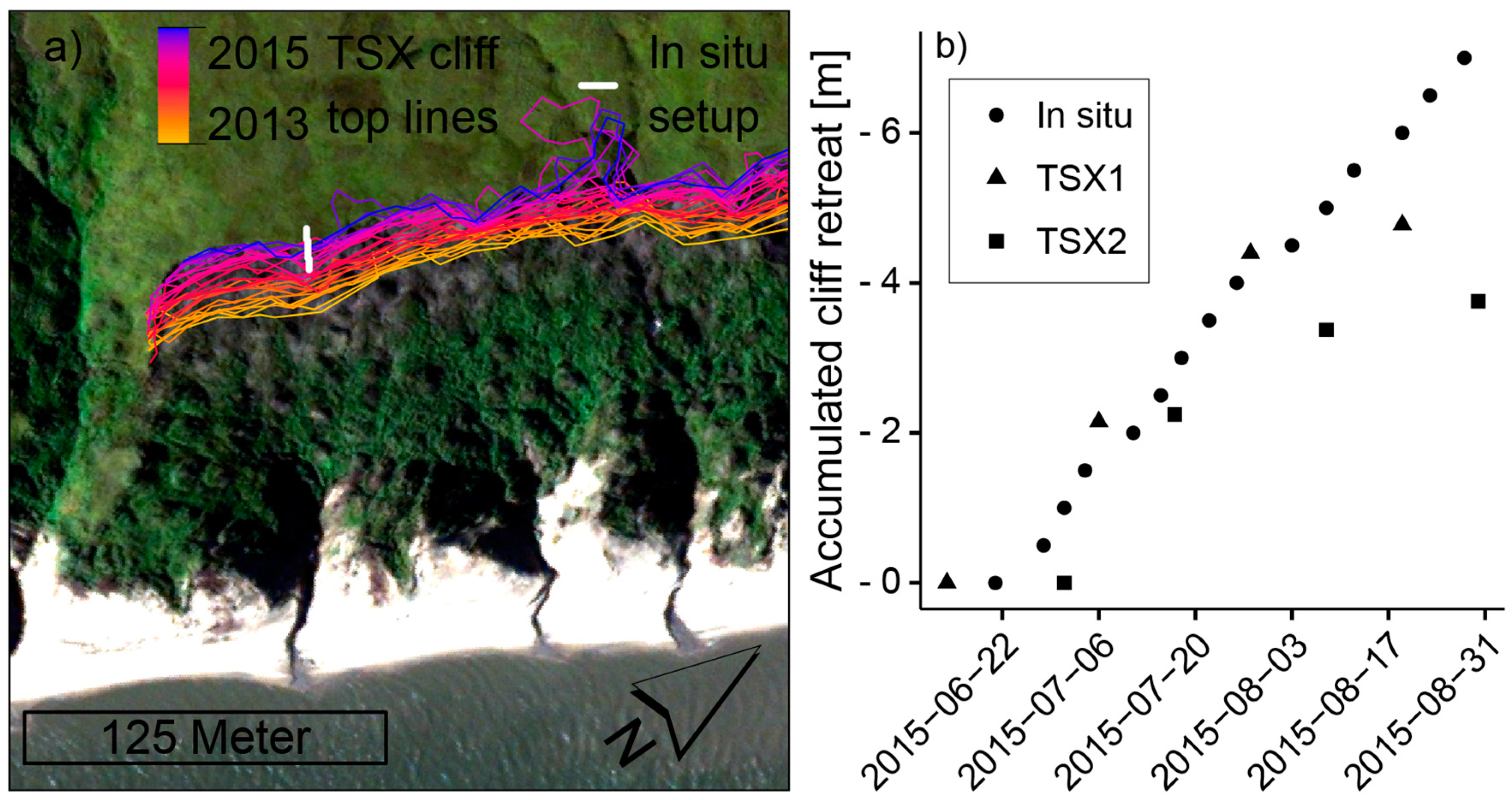
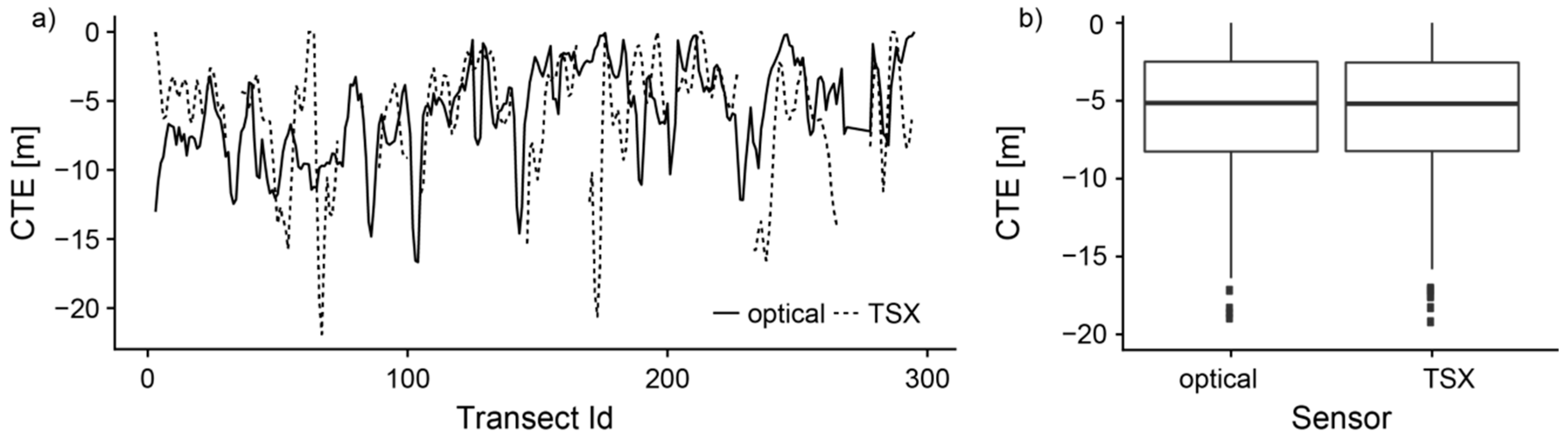
4.1. TSX Erosion versus In-Situ and Optical Datasets
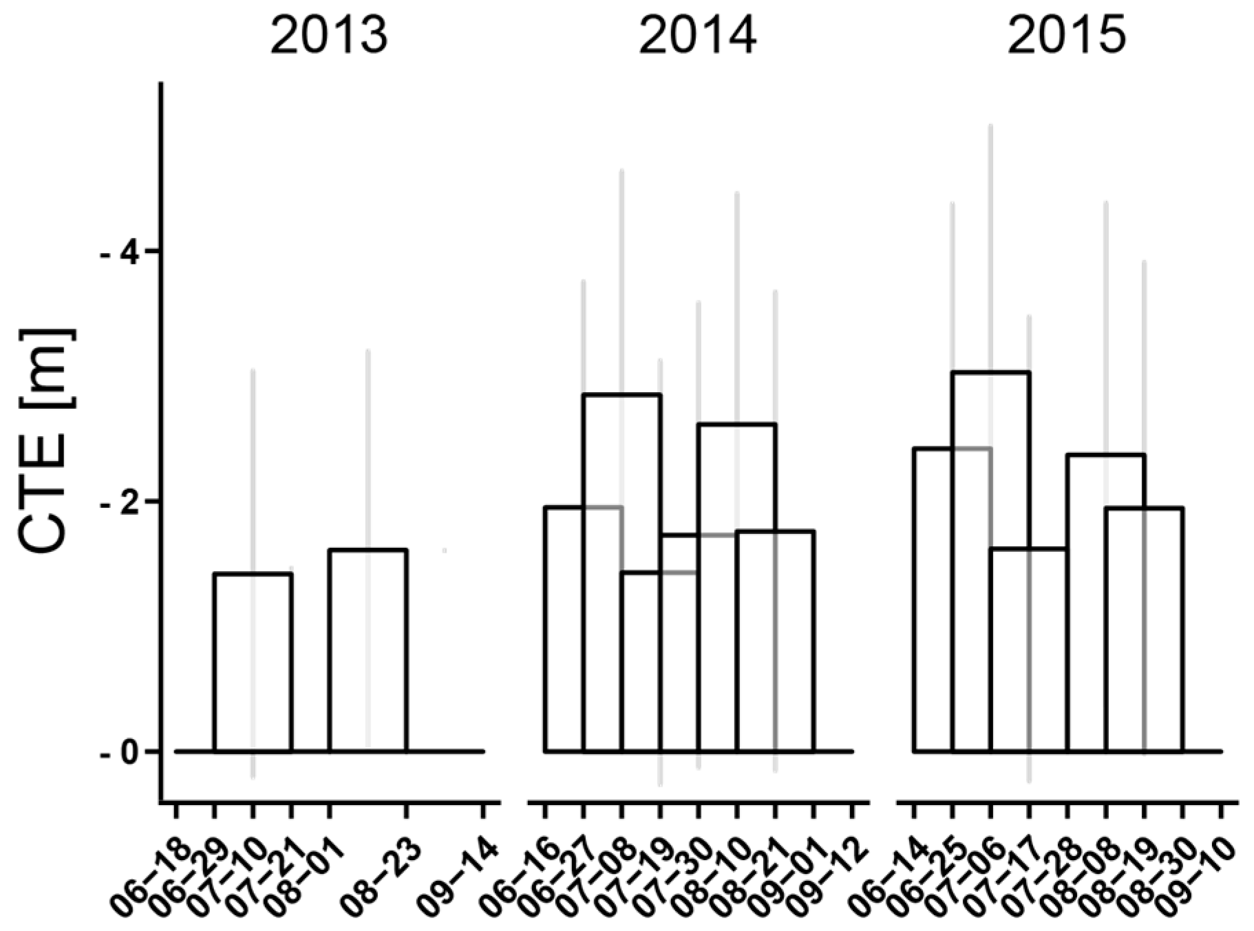
4.2. Inter- and Intra-Annual Cliff-Top Erosion and Climate Data
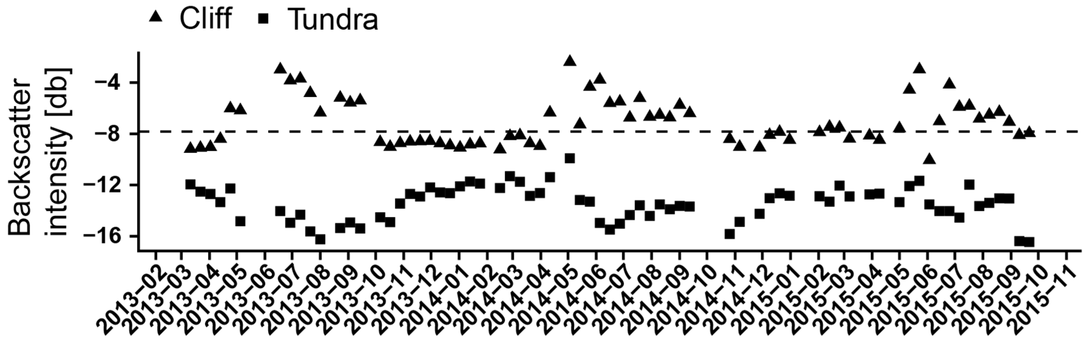
4.3. Backscatter Time Series
5. Discussion
5.1. Inter-Annual Dynamics of Cliff-Top Erosion
5.2. Intra-Annual Dynamics of Cliff-Top Erosion
5.3. Backscatter Dynamics of Tundra and Cliff Surfaces
6. Conclusions
Acknowledgments
Author Contributions
Conflicts of Interest
References
- AMAP. Snow, Water, Ice and Permafrost in the Arctic (SWIPA): Climate Change and the Cryosphere; AMAP: Oslo, Norway, 2011; p. 538. [Google Scholar]
- Romanovsky, V.E.; Smith, S.L.; Christiansen, H.H. Permafrost thermal state in the polar Northern Hemisphere during the international polar year 2007–2009: A synthesis. Permafr. Periglac. Process. 2010, 21, 106–116. [Google Scholar] [CrossRef]
- Grosse, G.; Harden, J.; Turetsky, M.; McGuire, A.D.; Camill, P.; Tarnocai, C.; Frolking, S.; Schuur, E.A.G.; Jorgenson, T.; Marchenko, S.; et al. Vulnerability of high-latitude soil organic carbon in North America to disturbance. J. Geophys. Res. 2011, 116. [Google Scholar] [CrossRef]
- Schuur, E.A.G.; McGuire, A.D.; Schadel, C.; Grosse, G.; Harden, J.W.; Hayes, D.J.; Hugelius, G.; Koven, C.D.; Kuhry, P.; Lawrence, D.M.; et al. Climate change and the permafrost carbon feedback. Nature 2015, 520, 171–179. [Google Scholar] [CrossRef] [PubMed]
- Liljedahl, A.K.; Boike, J.; Daanen, R.P.; Fedorov, A.N.; Frost, G.V.; Grosse, G.; Hinzman, L.D.; Iijma, Y.; Jorgenson, J.C.; Matveyeva, N.; et al. Pan-arctic ice-wedge degradation in warming permafrost and its influence on tundra hydrology. Nat. Geosci. 2016, 9, 312–318. [Google Scholar] [CrossRef]
- Subcommittee, P. Glossary of Permafrost and Related Ground-Ice Terms; Associate Committee on Geotechnical Research, National Research Council of Canada: Ottawa, ON, USA, 1988; p. 156. [Google Scholar]
- Lantuit, H.; Pollard, W.H.; Couture, N.; Fritz, M.; Schirrmeister, L.; Meyer, H.; Hubberten, H.W. Modern and Late Holocene retrogressive thaw slump activity on the Yukon coastal plain and Herschel Island, Yukon Territory, Canada. Permafr. Periglac. Process. 2012, 23, 39–51. [Google Scholar] [CrossRef]
- Morgenstern, A.; Grosse, G.; Günther, F.; Fedorova, I.; Schirrmeister, L. Spatial analyses of thermokarst lakes and basins in Yedoma landscapes of the Lena Delta. Cryosphere 2011, 5, 849–867. [Google Scholar] [CrossRef] [Green Version]
- Aré, F.E. Thermal abrasion of sea coasts (part I). Polar Geogr. Geol. 1988, 12, 1. [Google Scholar] [CrossRef]
- Shur, Y.L. The Upper Horizon of Permafrost and Thermokarst; USSR Academy of Sciences, Siberian Branch: Novosibirsk, Russia, 1988; p. 210. [Google Scholar]
- Kanevskiy, M.; Shur, Y.; Strauss, J.; Jorgenson, T.; Fortier, D.; Stephani, E.; Vasiliev, A. Patterns and rates of riverbank erosion involving ice-rich permafrost (Yedoma) in northern Alaska. Geomorphology 2016, 253, 370–384. [Google Scholar] [CrossRef]
- Walker, J.; Lennart, A.; Peippo, J. Riverbank erosion in the colville delta, Alaska. Geogr. Ann. 1987, 69, 61–70. [Google Scholar] [CrossRef]
- Costard, F.; Gautier, E.; Fedorov, A.; Konstantinov, P.; Dupeyrat, L. An assessment of the erosion potential of the fluvial thermal process during ice breakups of the Lena River (Siberia). Permafr. Periglac. Process. 2014, 25, 162–171. [Google Scholar] [CrossRef]
- Günther, F.; Overduin, P.P.; Sandakov, A.V.; Grosse, G.; Grigoriev, M.N. Short- and long-term thermo-erosion of ice-rich permafrost coasts in the Laptev Sea region. Biogeosciences 2013, 10, 4297–4318. [Google Scholar] [CrossRef] [Green Version]
- Jones, B.M.; Grosse, G.; Arp, C.D.; Jones, M.C.; Anthony, K.M.W.; Romanovsky, V.E. Modern thermokarst lake dynamics in the continuous permafrost zone, northern Seward Peninsula, Alaska. J. Geophys. Res. 2011, 116. [Google Scholar] [CrossRef]
- Morgenstern, A. Thermokarst and Thermal Erosion: Degradation of Siberian Ice-Rich Permafrost. Ph.D. Thesis, University of Potsdam, Potsdam, Germany, 2012. [Google Scholar]
- Scott, K.M. Effects of Permafrost on Stream Channel Behavior in Arctic Alaska; Geological Survey Professional Paper 1068; U.S. Department of the Interior: Washington, DC, USA, 1978; pp. 1–19.
- Tananaev, N.I. Hydrological and sedimentary controls over fluvial thermal erosion, the Lena River, central yakutia. Geomorphology 2016, 253, 524–533. [Google Scholar] [CrossRef]
- Shur, Y.; Vasiliev, A.; Kanevsky, M.; Maximov, V.; Pokrovsky, S.; Zaikanov, V. Shore erosion in Russian Arctic. In Cold Regions Engineering: Cold Regions Impacts on Transportation and Infrastructure; American Society of Civil Engineers: Anchorage, AK, USA, 2002. [Google Scholar]
- Günther, F.; Overduin, P.P.; Sandakov, A.V.; Grosse, G.; Grigoriev, M.N. Thermo-erosion along the Yedoma coast of the Buor Khaya Peninsula, Laptev Sea, East Siberia. In Proceedings of the 10th International Conference on Permafrost, Salekhard, Russia, 25–29 June 2012; Volume 2, pp. 137–142. [Google Scholar]
- Morgenstern, A.; Grosse, G.; Arcos, D.R.; Günther, F.; Overduin, P.P.; Schirrmeister, L. The role of thermal erosion in the degradation of Siberian ice-rich permafrost. J. Geophys. Res. 2014. under revision. [Google Scholar]
- Bartsch, A. Requirements for Monitoring of Permafrost in Polar Regions—A Community White Paper in Response to the WMO Polar Space Task Group (PSTG). Available online: http://www.wmo.int/pages/prog/sat/meetings/documents/PSTG-4_Doc_08-03_Permafrost-Recommendations-Final.pdf (accessed on 31 October 2017).
- Ullmann, T.; Schmitt, A.; Roth, A.; Duffe, J.; Dech, S.; Hubberten, H.-W.; Baumhauer, R. Land cover characterization and classification of arctic tundra environments by means of polarized synthetic aperture X- and C-Band radar (polsar) and Landsat 8 multispectral imagery—Richards Island, Canada. Remote Sens. 2014, 6, 8565–8593. [Google Scholar] [CrossRef]
- Widhalm, B.; Bartsch, A.; Heim, B. A novel approach for the characterization of tundra wetland regions with C-Band sar satellite data. Int. J. Remote Sens. 2015, 36, 5537–5556. [Google Scholar] [CrossRef] [PubMed] [Green Version]
- Short, N.; Brisco, B.; Couture, N.; Pollard, W.; Murnaghan, K.; Budkewitsch, P. A comparison of TerraSAR-X, RADARSAT-2 and ALOS-PALSAR interferometry for monitoring permafrost environments, case study from Herschel Island, Canada. Remote Sens. Environ. 2011, 115, 3491–3506. [Google Scholar] [CrossRef]
- Hogstrom, E.; Trofaier, A.M.; Gouttevin, I.; Bartsch, A. Assessing seasonal backscatter variations with respect to uncertainties in soil moisture retrieval in Siberian tundra regions. Remote Sens. 2014, 6, 8718–8738. [Google Scholar] [CrossRef]
- Antonova, S.; Kääb, A.; Heim, B.; Langer, M.; Boike, J. Spatio-temporal variability of X-Band radar backscatter and coherence over the Lena River Delta, Siberia. Remote Sens. Environ. 2016, 182, 169–191. [Google Scholar] [CrossRef]
- Notti, D.; Davalillo, J.C.; Herrera, G.; Mora, O. Assessment of the performance of X-Band satellite radar data for landslide mapping and monitoring: Upper Tena Valley case study. Nat. Hazards Earth Syst. Sci. 2010, 10, 1865–1875. [Google Scholar] [CrossRef] [Green Version]
- Strozzi, T.; Delaloye, R.; Kääb, A.; Ambrosi, C.; Perruchoud, E.; Wegmüller, U. Combined observations of rock mass movements using satellite SAR interferometry, differential GPS, airborne digital photogrammetry, and airborne photography interpretation. J. Geophys. Res. 2010, 115. [Google Scholar] [CrossRef]
- Zwieback, S.; Bartsch, A.; Boike, J.; Grosse, G.; Günther, F.; Heim, B.; Morgenstern, A.; Hajnsek, I. Monitoring permafrost and thermokarst processes with Tandem-x dem time series: Opportunities and limitations. In Proceedings of the IEEE International Geoscience and Remote Sensing Symposium (IGARSS), Beijing, China, 10–15 July 2016; pp. 332–335. [Google Scholar]
- Zwieback, S.; Kokelj, S.V.; Günther, F.; Boike, J.; Grosse, G.; Hajnsek, I. Sub-seasonal thaw slump mass wasting is not consistently energy limited at the landscape scale. Cryosphere Discuss. 2017, 1–24. [Google Scholar] [CrossRef]
- Ullmann, T.; Banks, S.N.; Schmitt, A.; Jagdhuber, T. Scattering characteristics of X-, C- and L-Band polsar data examined for the tundra environment of the Tuktoyaktuk Peninsula, Canada. Appl. Sci. 2017, 7, 595. [Google Scholar] [CrossRef]
- Walker, H.J. Arctic deltas. J. Coast. Res. 1998, 14, 718–738. [Google Scholar]
- Schneider, J.; Grosse, G.; Wagner, D. Land cover classification of tundra environments in the arctic Lena Delta based on Landsat 7 ETM+ data and its application for upscaling of methane emissions. Remote Sens. Environ. 2009, 113, 380–391. [Google Scholar] [CrossRef] [Green Version]
- Romanovskii, N.N.; Hubberten, H.W.; Gavrilov, A.V.; Tumskoy, V.E.; Kholodov, A.L. Permafrost of the east Siberian arctic shelf and coastal lowlands. Quat. Sci. Rev. 2004, 11, 1359–1369. [Google Scholar] [CrossRef] [Green Version]
- Boike, J.; Kattenstroth, B.; Abramova, K.; Bornemann, N.; Chetverova, A.; Fedorova, I.; Frob, K.; Grigoriev, M.; Gruber, M.; Kutzbach, L.; et al. Baseline characteristics of climate, permafrost and land cover from a new permafrost observatory in the Lena River Delta, Siberia (1998–2011). Biogeosciences 2013, 10, 2105–2128. [Google Scholar] [CrossRef] [Green Version]
- Grosse, G.; Robinson, J.E.; Bryant, R.; Taylor, M.D.; Harper, W.; DeMasi, A.; Kyker-Snowman, E.; Veremeeva, A.; Schirrmeister, L.; Harden, J. Distribution of Late Pleistocene Ice-Rich Syngenetic Permafrost of the Yedoma Suite in East and Central Siberia, Russia; Open File Report 2013-1078; U.S. Geological Survey: Reston, VA, USA, 2013; pp. 1–37.
- Strauss, J.; Schirrmeister, L.; Grosse, G.; Fortier, D.; Hugelius, G.; Knoblauch, C.; Romanovsky, V.; Schädel, C.; von Deimling, T.S.; Schuur, E.A.G.; et al. Deep Yedoma permafrost: A synthesis of depositional characteristics and carbon vulnerability. Earth-Sci. Rev. 2017, 172, 75–86. [Google Scholar] [CrossRef]
- Morgenstern, A.; Ulrich, M.; Günther, F.; Roessler, S.; Fedorova, I.V.; Rudaya, N.A.; Wetterich, S.; Boike, J.; Schirrmeister, L. Evolution of thermokarst in east Siberian ice-rich permafrost: A case study. Geomorphology 2013, 201, 363–379. [Google Scholar] [CrossRef]
- Grigoriev, M.N.; Rachold, V.; Bolshiyanov, D. Russian-German Cooperation System Laptev Sea: The Expedition Lena 2002; Alfred Wegener Institute for Polar and Marine Research: Bremerhaven, Germany, 2003; p. 341. [Google Scholar]
- Schirrmeister, L.; Grosse, G.; Schwamborn, G.; Andreev, A.A.; Meyer, H.; Kunitsky, V.V.; Kuznetsova, T.V.; Dorozhkina, M.V.; Pavlova, E.Y.; Bobrov, A.A.; et al. Late Quaternary history of the accumulation plain north of the Chekanovsky Ridge (Lena Delta, Russia): A multidisciplinary approach. Polar Geogr. 2003, 27, 277–319. [Google Scholar] [CrossRef]
- Wetterich, S.; Kuzmina, S.; Andreev, A.A.; Kienast, F.; Meyer, H.; Schirrmeister, L.; Kuznetsova, T.; Sierralta, M. Palaeoenvironmental dynamics inferred from Late Quaternary permafrost deposits on Kurungnakh island, Lena Delta, northeast Siberia, Russia. Quat. Sci. Rev. 2008, 27, 1523–1540. [Google Scholar] [CrossRef] [Green Version]
- Fedorova, I.; Chetverova, A.; Bolshiyanov, D.; Makarov, A.; Boike, J.; Heim, B.; Morgenstern, A.; Overduin, P.P.; Wegner, C.; Kashina, V.; et al. Lena Delta hydrology and geochemistry: Long-term hydrological data and recent field observations. Biogeosciences 2015, 12, 345–363. [Google Scholar] [CrossRef] [Green Version]
- Morgenstern, A.; Röhr, C.; Grosse, G.; Grigoriev, M.N. The Lena River Delta—Inventory of Lakes and Geomorphological Terraces; Alfred Wegener Institute—Research Unit Potsdam: Potsdam, Germany, 2011. [Google Scholar]
- ESA. Sentinel Application Platform (SNAP) Version 3.0. Available online: http://step.esa.int (accessed on 20 November 2017).
- Douglas, D.H.; Peucker, T.K. Algorithms for the reduction of the number of points required to represent a digitized line or its caricature. Cartogr. Int. J. Geogr. Inf. Geovis. 1973, 10, 112–122. [Google Scholar] [CrossRef]
- Thieler, E.R.; Himmelstoss, E.A.; Zichichi, J.L.; Ergul, A. Digital Shoreline Analysis System (DSAS) Version 4.0—An ArcGIS extension for Calculating Shoreline Change; Open-File Report 2008-1278; U.S. Geological Survey: Reston, VA, USA, 2009.
- Fraser, C.S.; Ravanbakhsh, M. Georeferencing accuracy of Geoeye-1 imagery. Photogramm. Eng. Remote Sens. 2009, 75, 634–638. [Google Scholar]
- Stettner, S. Characterizing Thermo-Erosional Landforms in Siberian Ice-Rich Permafrost. Morphometric Investigations in the Lena Delta Using High-Resolution Satellite Imagery and Digital Elevation Models. Master’s Thesis, Freie Universität Berlin, Berlin, Germany, 2014. [Google Scholar]
- R Core Team. R: A Language and Environment for Statistical Computing; R Foundation for Statistical Computing: Vienna, Austria, 2016. [Google Scholar]
- Bates, D.; Mächler, M.; Bolker, B.; Walker, S. Fitting linear mixed-effects models using lme4. J. Stat. Softw. 2015, 67. [Google Scholar] [CrossRef]
- Schuur, E.A.G.; Bockheim, J.; Canadell, J.G.; Euskirchen, E.; Field, C.B.; Goryachkin, S.V.; Hagemann, S.; Kuhry, P.; Lafleur, P.M.; Lee, H.; et al. Vulnerability of permafrost carbon to climate change: Implications for the global carbon cycle. Bioscience 2008, 58, 701–714. [Google Scholar] [CrossRef]
- Kokelj, S.V.; Tunnicliffe, J.; Lacelle, D.; Lantz, T.C.; Chin, K.S.; Fraser, R. Increased precipitation drives mega slump development and destabilization of ice-rich permafrost terrain, Northwestern Canada. Glob. Planet. Chang. 2015, 129, 56–68. [Google Scholar] [CrossRef]
- Dupeyrat, L.; Costard, F.; Randriamazaoro, R.; Gailhardis, E.; Gautier, E.; Fedorov, A. Effects of ice content on the thermal erosion of permafrost: Implications for coastal and fluvial erosion. Permafr. Periglac. Process. 2011, 22, 179–187. [Google Scholar] [CrossRef]
- Ramage, J.L.; Irrgang, A.M.; Herzschuh, U.; Morgenstern, A.; Couture, N.; Lantuit, H. Terrain controls on the occurrence of coastal retrogressive thaw slumps along the Yukon Coast, Canada. J. Geophys. Res. Earth Surf. 2017, 122, 1619–1634. [Google Scholar] [CrossRef]
- Duguay, Y.; Bernier, M.; Lévesque, E.; Tremblay, B. Potential of C and X-Band SAR for shrub growth monitoring in sub-arctic environments. Remote Sens. 2015, 7, 9410–9430. [Google Scholar] [CrossRef]
- Gorrab, A.; Zribi, M.; Baghdadi, N.; Mougenot, B.; Fanise, P.; Chabaane, Z. Retrieval of both soil moisture and texture using TerraSAR-X images. Remote Sens. 2015, 7, 10098–10116. [Google Scholar] [CrossRef] [Green Version]
- Shi, X.; Zhang, L.; Tang, M.; Li, M.; Liao, M. Investigating a reservoir bank slope displacement history with multi-frequency satellite SAR data. Landslides 2017, 14, 1961–1973. [Google Scholar] [CrossRef]
- Eriksen, H.Ø.; Lauknes, T.R.; Larsen, Y.; Corner, G.D.; Bergh, S.G.; Dehls, J.; Kierulf, H.P. Visualizing and interpreting surface displacement patterns on unstable slopes using multi-geometry satellite SAR interferometry (2D InSAR). Remote Sens. Environ. 2017, 191, 297–312. [Google Scholar] [CrossRef]


| Sensor | Observation Start (yyyy-mm-dd) | Observation End (yyyy-mm-dd) | Days above 0 °C | Net CTE (m) | Theoretical Cliff-Top Erosion Rate (m/day) |
|---|---|---|---|---|---|
| In situ | 2015-06-21 | 2015-08-30 | 71 | −7.0 | 0.09 |
| TSX | 2015-06-25 | 2015-08-30 | 67 | −5.19 | 0.07 |
| Sensor | Observation Start (yyyy-mm-dd) | Observation End (yyyy-mm-dd) | Days above 0 °C | Mean Net CTE (m) | Theoretical Cliff-Top Erosion Rate (m/day) |
|---|---|---|---|---|---|
| Optical | 2014-08-19 | 2015-08-26 | 126 | −5.78 ± 4.45 | 0.04 |
| TSX | 2014-08-21 | 2015-08-30 | 128 | −6.92 ± 6.31 | 0.05 |
| 2013 | 2014 | 2015 | Long Term Mean * | |
|---|---|---|---|---|
| Mean CTE per 22-day (m) | −1.37 ± 1.55 a | −1.96 ± 1.85 b | −1.85 ± 1.97 c | |
| Median CTE per 22-day (m) | −1.24 | −1.9 | −1.49 | |
| Mean net CTE (m) | −4.1 ± 3.7 (88 days) a | −6.9 ± 4.6 (88 days) b | −5.1 ± 5.3 (66 days) c | |
| Mean Temperature (°C) (June to September) | 6.1 ± 4.8 a | 7.6 ± 4.7 b | 6.4 ± 4.4 ab | 6.4 ± 3.4 (1998–2014) |
| Thawing-degree days (June to September) | 691.9 | 824.2 | 628.9 | 790 ± 120 (1998–2014) |
| Mean incoming short wave radiation (W/m2) (June to September) | 133 ± 87.2 a | 141.4 ± 91 a | 130.9 ± 81.7 a | - |
| Mean Precipitation (mm) (June to September) | 0.9 ± 2.6 a | 0.8 ± 1.6 a | 1.1 ± 2.9 a | 1.3 ± 3.1 (1998–2008) |
| Precipitation sum (mm) (June to September) | 109 | 104 | 146 | 124 ± 69 (1998–2008) |
| No of extreme precipitation events >15/10/5 mm (June to September) | 2/3/5 | 0/0/5 | 2/5/8 | 1.45 ± 1.30/2.58 ± 1.83/ 6.5 ± 4.23 (1998–2008) |
| Year | Fixed Effects | Random Effects | AIC | BIC | p-Value |
|---|---|---|---|---|---|
| 2013 | CTE~SWIN + P + TDD | MD + TID | 7138.6 | 7138.6 | <0.01 |
| 2014 | CTE~P | MD + TID | 10,993.4 | 1102.9 | >0.05 |
| 2015 | CTE~SWIN + P | MD + TID | 10,962.7 | 10,998.0 | <0.05 |
| AOI | 2013 | 2014 | 2015 | All | |
|---|---|---|---|---|---|
| Mean summer backscatter | Tundra | −16.29 ± 6.53 a | −15.62 ± 6.47 b | −14.81 ± 6.47 c | −15.50 ± 6.51 |
| cliff | −5.29 ±6.65 a | −6.88 ± 6.93 b | −6.69 ± 7.05 c | −6.39 ± 6.93 |
© 2017 by the authors. Licensee MDPI, Basel, Switzerland. This article is an open access article distributed under the terms and conditions of the Creative Commons Attribution (CC BY) license (http://creativecommons.org/licenses/by/4.0/).
Share and Cite
Stettner, S.; Beamish, A.L.; Bartsch, A.; Heim, B.; Grosse, G.; Roth, A.; Lantuit, H. Monitoring Inter- and Intra-Seasonal Dynamics of Rapidly Degrading Ice-Rich Permafrost Riverbanks in the Lena Delta with TerraSAR-X Time Series. Remote Sens. 2018, 10, 51. https://doi.org/10.3390/rs10010051
Stettner S, Beamish AL, Bartsch A, Heim B, Grosse G, Roth A, Lantuit H. Monitoring Inter- and Intra-Seasonal Dynamics of Rapidly Degrading Ice-Rich Permafrost Riverbanks in the Lena Delta with TerraSAR-X Time Series. Remote Sensing. 2018; 10(1):51. https://doi.org/10.3390/rs10010051
Chicago/Turabian StyleStettner, Samuel, Alison L. Beamish, Annett Bartsch, Birgit Heim, Guido Grosse, Achim Roth, and Hugues Lantuit. 2018. "Monitoring Inter- and Intra-Seasonal Dynamics of Rapidly Degrading Ice-Rich Permafrost Riverbanks in the Lena Delta with TerraSAR-X Time Series" Remote Sensing 10, no. 1: 51. https://doi.org/10.3390/rs10010051