3-D Water Vapor Tomography in Wuhan from GPS, BDS and GLONASS Observations


1
Shanghai Key Laboratory of Space Navigation and Positioning Techniques, Shanghai Astronomical Observatory, Chinese Academy of Sciences, Shanghai 200030, China
2
University of Chinese Academy of Sciences, Beijing 100049, China
3
Department of Geomatics Engineering, Bulent Ecevit University, Zonguldak 67100, Turkey
4
Geospheric Activities and Atmospheric Variations Lab, Harbin Institute of Technology, Shenzhen 518000, China
*
Author to whom correspondence should be addressed.
Remote Sens. 2018, 10(1), 62; https://doi.org/10.3390/rs10010062
Submission received: 6 December 2017
/
Revised: 2 January 2018
/
Accepted: 3 January 2018
/
Published: 4 January 2018
(This article belongs to the Special Issue Multi-Constellation Global Navigation Satellite Systems: Methods and Applications)
Abstract
:Three-dimensional water vapor can be reconstructed from Global Navigation Satellite System (GNSS) observations, which can study 3-D profile variations of atmospheric water vapor and climate. However, there is a large uncertainty of water vapor tomography from single GPS system observations due to limited satellites. The rapid development of multi-GNSS, including China’s Beidou Navigation Satellite System (BDS) and Russia’s GLONASS, has greatly improved the geometric distribution of satellite ray-path signals, which may improve the performance of water vapor tomography by combining multi-GNSS. In this paper, 3-D water vapor tomography results are the first time obtained using multi-GNSS data from Continuously Operating Reference Stations (CORS) network in Wuhan, China, whose performances are validated by radiosonde and the latest ECMWF ERA5 reanalysis products. The results show that the integrated multi-GNSS can pronouncedly increase the number of effective signals, and 3-D water vapor results are better than those from the GPS-only system, improving by 5% with GPS + GLONASS or GPS + GLONASS + BDS, while BDS has results that are not improved too much. Therefore, multi-GNSS will enhance the reliability and accuracy of 3-D water vapor tomography, which has more potential applications in the future.
1. Introduction
The distribution and variations of atmospheric water vapor are related to various weathers and climate changes and, hence, water vapor has always been an extremely important observation in these fields. Since Bevis et al. [1] proposed to remotely sense atmospheric water vapor using the Global Positioning System (GPS), after more than 20 years of sustainable development GPS meteorology has become a significant approach for water vapor detection with its advantages of continuous observations, high accuracy and temporal-spatial resolution, high cost-benefit, and so on [2,3,4,5]. The spatial distribution of 3-D or 4-D water vapor can be obtained by tomographic techniques through the dense ground-based GPS station network, which will benefit numeric weather prediction together with assimilation methods, the study of water vapor transport during precipitation, and even the nowcasting of extreme disastrous weather. However, it has a large uncertainty of water vapor tomography from single-system GPS observations due to limited satellites. Nowadays, with the rapid development of Global Navigation Satellite Systems (GNSS), we have entered the era of GNSS meteorology, and the integration of multi-GNSS tropospheric tomography will provide more inversion signals, which may improve water vapor tomography in comparison with GPS-only systems.
Although previous studies have proved that GPS tropospheric tomography is a promising technique to remotely sense the temporal-spatial distribution of water vapor [6,7,8,9], GNSS tomography is still in the experimental stage due to the low accuracy and limited ray-path signals [10]. Different grid tomography optimization methods and inversion signal utilization methods have been proposed to improve the quality of tomographic water vapor fields [11,12]. Combining with other water vapor observation technologies, including radiosondes, water vapor radiometers, sun photometers, and even COSMIC and MODIS, can provide additional inversion information [13,14], but their contributions are still limited and also difficult to carry out in practice due to the restriction of these technologies, themselves, such as the cost, the quality of observations, and the temporal-spatial resolution of the observations. With the significant progress of BDS and Galileo systems, as well as updating GLONASS, the integrated multi-GNSS may improve water vapor tomography [15,16].
In this paper, 3-D tropospheric water vapor tomography is estimated with observed multi-GNSS data, which is validated by radiosonde and the latest reanalysis ERA5 products from ECMWF. In Section 2, methods of 3-D water vapor tomography are introduced, the results from different GNSS systems are presented in Section 3, a discussion is offered in Section 4, and, finally, conclusions are given in Section 5.
2. GNSS Observations and Methods
2.1. GNSS Tropospheric Estimation
The tropospheric zenith total delay (ZTD) can be obtained from GNSS observations, including the zenith hydrostatic delay (ZHD) and zenith wet delay (ZWD). The ZHD can be precisely calculated by atmospheric models or surface meteorological parameters, and the zenith wet delay (ZWD) can be obtained by subtracting ZHD from ZTD, namely:
There is a linear relationship between ZWD and precipitable water vapor (PWV) [4]:
where Π is the conversion factor between ZWD and PWV. The physical sense of PWV represents the height at which water vapor in the atmosphere column of the unit bottom reaches saturation and condenses into liquid water. Π is a function of the mean temperature of the water vapor Tm:
where ρw is the density of liquid water, R is the universal gas constant (R = 8314 Pa·m3·K−1·kmol−1), mw is the molar mass of water (mw = 18.02 kg/kmol), md represents the molar mass of the dry atmosphere (md = 28.96 kg/kmol), k1, k2, and k3 are empirical physical constants (k1 = 77.604 K/hPa, k2 = 70.4 K/hPa, k3 = 3.776 × 10⁵ K2/hPa), and Tm is related to the temperature and vapor pressure at different altitudes in the atmosphere. In practice, an empirical formula for surface temperature and Tm is established by linear regression analysis using long-term radiosonde data [1].
The observations of the tropospheric water vapor tomography are the integration of water vapor in the direction of the ray-path slant water vapor (SWV) which can be expressed as:
where ρ(l) represents the water vapor density, dl specifies the length of a signal element, Mw is the wet mapping coefficient, and the last term R refers to the non-homogeneous variation of water vapor, which is calculated by multiplying the post-fit residual by the conversion factor.
2.2. Tomographic observation model
The principle of tomography technique is to use the integral observations to reconstruct the detailed information of the studied objects through a certain mathematical constraint. In GNSS meteorology, the integral observations of tropospheric tomography are SWV, with the movement of satellites in space and the rotation of Earth, and dense GNSS observations can retrieve the 3-D water vapor over the interested area with the tomography technique.
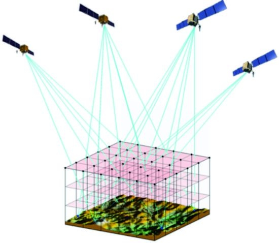
To solve the integral problem of total water vapor, the discretized method is adopted in GNSS water vapor tomography. Based on the voxel-based method, the tropospheric zone over the interested area is discretized into the self-enclosed 3-D voxels in horizontal and vertical directions (Figure 1). Due to the limited number of ground stations, the total number of tomographic signals at single epoch is not enough and, therefore, it usually requires accumulating observation signals for a period time, which is called tomography window, so the inversion field is the average of the water vapor distribution over this period time. Assumed that the water vapor parameters of each voxel at epoch t are represented by X(r, t), where r stands for the position of voxels, the slant water vapor (SWV) for signal p in a single tomography window can be described as:
where dl represents the intercept of the signal p at the r voxel.
Although we assumed that the water vapor status remains stationary in a tomography window and the number of accumulated tomography signals will be much larger than the total number of voxels, the tropospheric tomographic observation equations are still ill-posed as some voxels always have no signal passing due to the limited spatial distribution of satellites and stations on the ground network. Thus, the observation equations cannot be solved directly by the least square (LS) estimation. In order to solve the inversion problem of the singular design matrix in the tomography model, constraints are introduced into the observation model. It is supposed that there is a spatial correlation between the atmospheric water vapor in a specific voxel and surrounding voxels. The common methods of constraints include the horizontal constraint, vertical constraint, and boundary constraint [6,17].
In the same layer of the grid, it is assumed that there is a Gaussian inverse distance weighted relationship between the water vapor density of a voxel and the other voxels. The Gaussian distance weighting function has the following form:
where (i, j) represents the voxel location calculated at a certain layer of the grid, (i1, j1) stands for a nearby voxel, di1, j1 represents the distance from voxel (i, j) to (i1, j1), nl and nn are the number of the grid divided in the latitude and longitude directions, and δ is a Gaussian smoothing factor, which is determined according to the range of smoothing assumptions.
A priori water vapor distribution information is used to establish the vertical constraints [13,18] to solve the alteration phenomenon of inversion water vapor field that upper water vapor density is smaller than water vapor density at the bottom. In addition, the top boundary constraint can also be added to force the water vapor density of voxels at the topper layer to zeros. Then, the tomography model can be described as:
where y is a column vector composed of all GNSS SWV in a single tomography window, AGNSS is the design matrix composed of GNSS signal intercepts at each voxel, H, V, and B are the coefficient matrices for the horizontal, vertical, and top boundary constraints, r represents the prior water density provided by external observation techniques, and ε is the residual.
The design matrix of tomography equation established by GNSS technique and constraint equations is a large-scale sparse matrix and, in fact, the tomography solution is the inverse problem of the coefficient matrix. In order to ensure the physical sense of the solution, the results of the equations must be positive. The solving methods of tomography equations include the non-iterative algorithm, iterative algorithm and the joint approach of both. Non-iterative methods, such as LS, singular value decomposition (SVD), etc., are not sensitive to initial values, and only approximate values can be obtained. The iterative reconstruction method requires a higher precision initial value to converge, and the accuracy of the corresponding solution is also higher. Bender et al. [19] compared different iterative reconstruction algorithms, and the results showed that the multiplicative algebraic reconstruction technique (MART) has better iterative accuracy and iterative speed. The MART algorithm is given by the following expression [20,21]:
where swvi and Ai represent the ith observation of the GNSS tomography equations and the corresponding vector of equation coefficients, the inner product is the back projection of ith GNSS tomography observation after the kth iteration, and λ is the relaxation parameter, which gives the weight correction rate. MART algorithm can be divided into two steps, firstly, the water vapor density of voxels (index j, j = 1, 2, …, m) is corrected one by one for each observation (index i, i = 1, 2, …, n), and then the next iteration is performed (index k, k = 1, 2, …, p) until the solution converges. Balancing the advantages and disadvantages of non-iterative and iterative approaches, a combined method has been demonstrated [22]. In this paper, the combined method is adopted, and SVD is implemented to obtain the approximate solution as the initial value of MART.
3. Results and Analysis
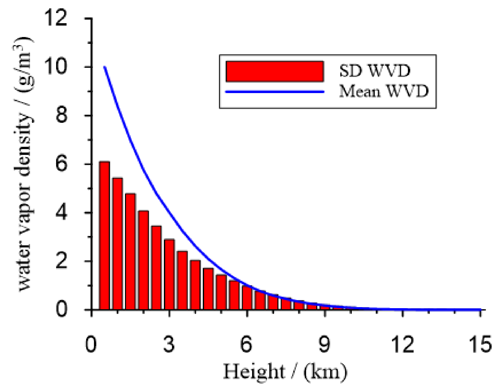
The tropospheric water vapor tomography is carried out from GPS system alone, GPS + BDS, GPS + GLONASS, and GPS + BDS + GLONASS. The multi-GNSS observations are from seven stations in Wuhan, China from day of year (DOY) 170 to 176, 2014. The station information is listed in Table 1, it should be noted that there are only six GNSS stations for DOY 170 and 175 because of missing data. The weather conditions are shown in Table 1 during the experiment, while the wind speed is less than 12 km/h per day. The average distance between seven stations is 18 km. According to the distribution of seven stations, the range of the studied areas in this tomography experiment is 30.25°N–30.9°N in latitude, 114.00°E–114.90°E in longitude, and the horizontal resolution is 0.13° in latitude and 0.18° in longitude. The spatial resolution of the east-west direction is about 17 km and about 14 km in south-north direction. The statistical results of radiosonde water vapor density profiles below 15 km from the year of 2004 to 2013 at radiosonde station 57,494 are shown in Figure 2, which gives the statistical mean value and standard deviation (SD) of water vapor density at different altitude.
We can find the average water vapor density and SD are close to 0 at the 10 km, and, therefore, 10 km is regarded as the top boundary of the water vapor layer, and the water vapor density in the vertical direction greater than 10 km is regarded as 0 g/m3. As Chen and Liu [11] stated, the non-uniform division method in the vertical direction is more consistent with the spatial distribution characteristics of water vapor. The troposphere from the ground surface to 10 km is set as 10 layers with a thickness of 500 m, five layers of 800 m and one layer of 1000 m. Hence, the total number of voxels is 5 × 5 × 16. The selected GNSS stations and the radiosonde station are shown in Figure 3.
During the experiment, 32 GPS satellites and 24 GLONASS satellites were operating normally, as were 14 BDS satellites, because the BDS geostationary Earth orbit (GEO) satellites have a relatively low accuracy of orbit determination and CODE (Center for Orbit Determination in Europe) did not provide their precise orbit and clock products, which are excluded from the experiment. The GNSS data sampling rate is 30 s, and the satellite cut-off angle is set at 10°. The multi-GNSS precise point positioning (PPP) is adopted to estimate the tropospheric delay using dual-frequency observations from GPS L1/L2, GLONASS G1/G2, and BDS B1/B2 observations, and the tropospheric zenith wet delay is modeled as a random walk process. The multi-constellation precise satellite orbit and clock products provided by CODE are employed to mitigate the satellite orbit and clock errors. IGS absolute model is applied to correct phase center offset (PCO) and variation (PCV) for GPS, GLONASS satellites and GNSS receiver, and BDS PCO are corrected with antenna offsets recommended by MGEX. To avoid the satellite-specific code hardware delay of GLONASS satellites, GLONASS pseudo-range observations are not used. Due to the difference of time datums for different GNSS systems, the system time difference is estimated as an unknown parameter. Other model corrections are performed as IGS suggested. The observations are weighted with satellite elevation angles, but different initial weights are assigned to different GNSS systems. The initial weight ratios of GPS, GLONASS, and BDS system are set to 2:1:2. The details of GNSS data processing are shown in Cai et al. [23].
The linear regression formula for surface temperature Ts and the mean temperature of the water vapor Tm obtained from radiosonde data at radiosonde station 57,494 from 2004 to 2013 is: , which is used for computing the conversion factor of water vapor. The average water vapor profile from three-day radiosonde data prior to the tomographic time is adopted as vertical prior information for the tomography [13], and the size of the tomography window is set to 0.5 h.
The corresponding radiosonde data and the latest ERA5 reanalysis products provided by the European Center for Medium Range Weather Forecasts (ECMWF) are used for external validation for the tomographic fields. Here, only one radiosonde station is available in the tomography area. The radiosonde usually launches two sounding balloons at UTC 00:00 and 12:00 each day, which is considered the most accurate method for water vapor detection. The ERA5 is the fifth generation of ECMWF atmospheric reanalysis of the global climate from 1950 to present. The first seven-year segment of the dataset from 2010 to 2016 is available free to public users now, and the whole dataset is gradually released over the next two years and continues to be updated forward in near real-time later. ERA5 provides hourly estimates of atmospheric, land, and oceanic climate variables with uncertainties. The data cover the Earth on a 30 km grid and resolve the atmosphere using 137 levels from the surface up to a height of 80 km, which will eventually replace the ERA-Interim reanalysis. Due to a lack of observed meteorological parameters around GNSS stations, surface pressure and temperature data used to calculate ZHD and Π are also provided by ERA5 surface products. The temporal resolution of ERA5 reanalysis products is 1 h, so the statistics of tomographic results and ERA5 are considered at 1 h interval in the later sections.
3.1. Comparison of GNSS Tomographic Results
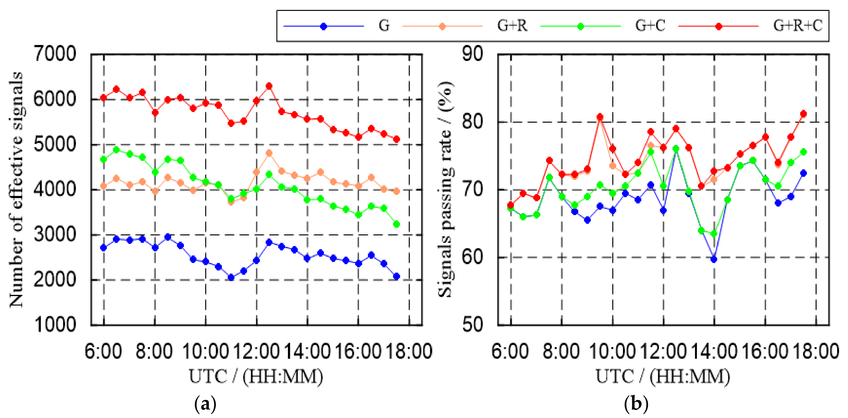
Figure 4 shows the effective SWV signals and the percentage of voxels crossed by effective signals of different GNSS systems in each tomography window from UTC 6:00 to 18:00 on DOY 171, 2014. G represents GPS-only tomographic signals in tomography experiments, G + R means the GPS and GLONASS integrated tomography system, G + C stands for the GPS and BDS combined tomography system, and G + R + C indicates that the GPS, GLONASS, and BDS are jointly used for tomography. As shown in Figure 4a, compared with the GPS-only tomography experiment, the number of GPS + GLONASS and GPS + BDS tomography signals is increased by 1.6 times, although there are significantly more GLONASS satellites than BDS satellites, more BDS satellites can be observed in the Asia-Pacific region due to current constellation optimization, while the combined triple-system is increased 2.2 times. Figure 4b shows the percentage of voxels crossed by signals of the integrated multi-GNSS system, which is better than the GPS-only system, and the increase in the voxel passing rate means that more voxels have the direct observations in the processing of reconstruction, which can obviously enhance the accuracy and reliability of the water vapor density inversion. The percentage of voxels crossed by signals from GPS + GLONASS systems is better than GPS + BDS, and the triple-system is slightly better than GPS + GLONASS. The average grid passing rate of seven days during our experiment was calculated as 69% for GPS-only, 74% for GPS + GLONASS, 71% for GPS + BDS, and 75% for GPS + GLONASS + BDS. It can be seen that the improvement of the grid passing rate of combined GNSS systems is unapparent.
3.2. Tomographic Profile Validation
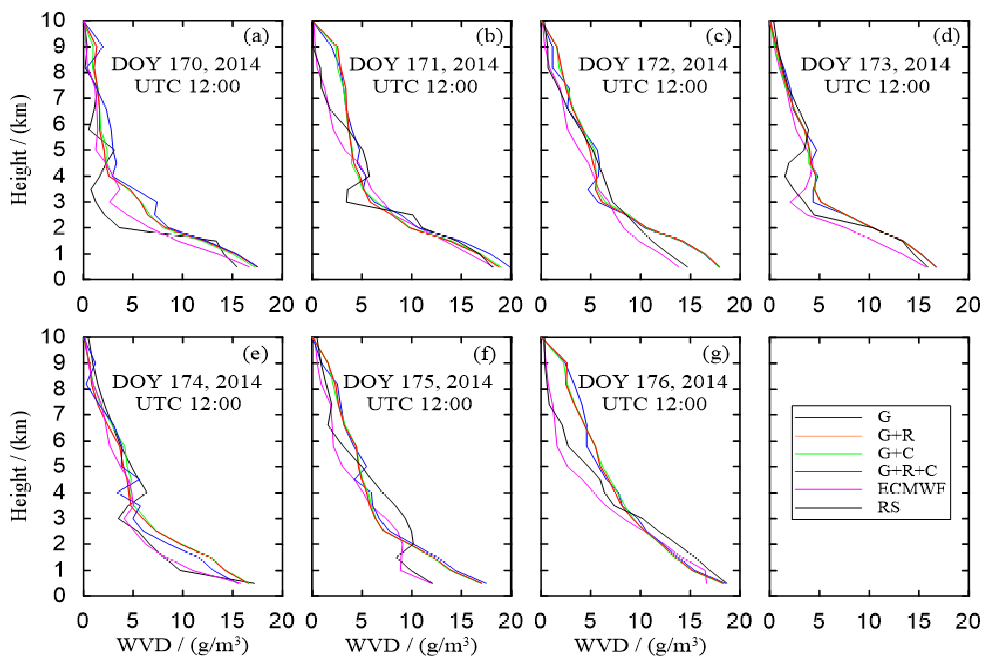
The advantage of tomography technique can obtain the vertical profile of water vapor density. Figure 5 shows the water vapor density profiles over the radiosonde station retrieved from tropospheric tomography in the four different GNSS systems, radiosonde data, and ERA5 reanalysis products. There is a good consistency between three types of water vapor density profiles, but the integrated multi-GNSS does not significantly improve the accuracy of the profiles. The inversion profiles on the day of year 171 and 176 show an obvious deviation above 6 km, and the main reason is the missing surface meteorological data in the tomographic experiment. At the same time, the precipitation is frequent during our tomographic experiment, which may cause a large model error.
Figure 6 shows the comparison of RMS and relative error between water vapor densities derived from ERA5 and different GNSS tomographic results from UTC 6:00 to 18:00 for seven days at different layers. Since the water vapor content decreases with the increase of the height, as shown in Figure 6a, the RMS of the different grid layers generally shows a decreasing trend with the height, and the RMS of the dual-system and triple-system are very close, both better than the GPS alone. The maximum RMS appears between 1 km to 1.5 km with 2.28 g/m3, 2.22 g/m3, 2.24 g/m3, and 2.22 g/m3 for GPS-only, GPS + GLONASS, GPS + BDS, and GPS + GLONASS + BDS, respectively. Table 2 lists the average Pearson correlations between GNSS tropospheric profiles and ERA5 profiles. The average Pearson correlation f is 96.4% for the integrated GNSS tomographic profiles and 95.9% for the GPS-only system. It can be found that the deviation of the RMS between combined systems and the GPS-only system increases with the increase of the layer height, and the relative error also exists in Figure 6b, which appears as large relative errors above 5 km, especially greater than 100% above 7 km. The main reason for this phenomenon is that the water vapor mainly concentrates below 5 km near the Earth’s surface. Additionally, the 10 years of statistical results from radiosonde data mentioned above show that water vapor content accounts for 90.4% below 5 km near the Earth’s surface, so the error between tomography and ERA5 easily masks the real weak water vapor information in the voxels of the upper layers.
3.3. Water Vapor Density Evaluation
Using ERA5 reanalysis products as the reference water vapor density of each voxel, the statistical GNSS tomographic results for seven days are listed in Table 3. The daily MAE and RMS of GPS-only tomographic results are worse than multi-GNSS tomography systems, while the statistical values of integrated systems are very close. Linear regression analysis of water vapor density from GNSS tomography and ERA5 reanalysis products was carried out. Figure 7a–d represent the regression results of GPS-only, GPS + BDS, GPS + GLONASS, and GPS + GLONASS + BDS, respectively. The bias, MAE, and RMS of GPS-only tomography are 0.92 g/m3, 1.42 g/m3, and 1.57 g/m3, respectively, and the slope of the linear regression equation is 0.95. The bias for GPS + GLONASS, GPS + BDS, and GPS + GLONASS + BDS are 0.87 g/m3, 0.87 g/m3, and 0.88 g/m3, respectively, and the RMS are 1.49 g/m3, 1.50 g/m3, 1.49 g/m3, respectively. The regression analysis indicates that the inversion accuracy of integrated multi-GNSS systems is improved by 5%, on average, when compared to GPS alone, while integrated multi-GNSS tomographic results are almost similar, indicating that the tomographic accuracy can be improved from GPS system to dual-system, while dual-system and triple-system have not too much improvement. Table 4 shows the total statistical results for seven days below 5 km since the water vapor is mainly concentrated below 5 km near the Earth surface. The RMS of tomographic water vapor density is 1.77 g/m3 for GPS + BDS, and the RMS of GPS + GLONASS and GPS + GLONASS + BDS are both 1.76 g/m3. Therefore, the accuracy is improved by 3% on average in comparison with GPS-only. The improvement of integrated multi-GNSS tomographic water vapor density below 5 km is less than the overall improvement rate.
3.4. PWV Validation
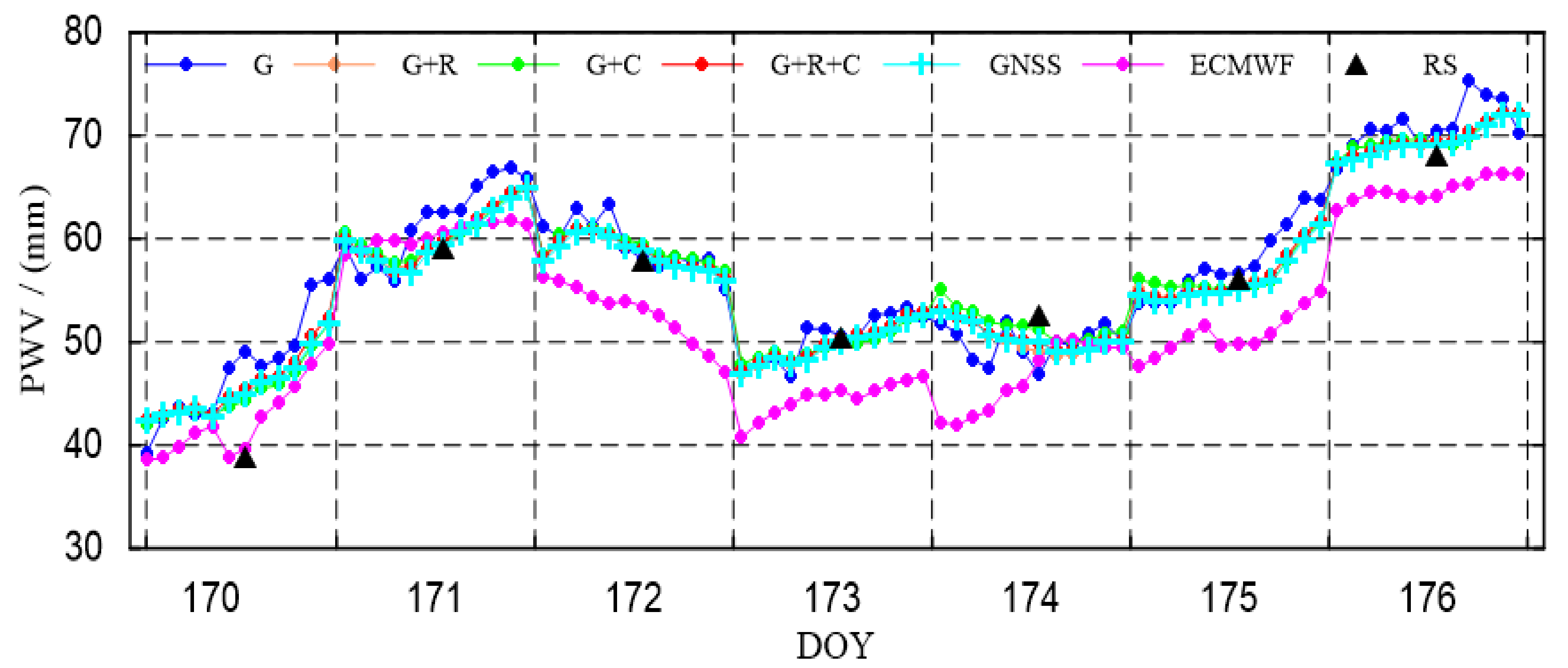
In order to further compare the accuracy of different GNSS systems, the tomographic results are evaluated by PWV derived from ERA5 surface reanalysis products from UTC 6:00 to 18:00 for seven days. Figure 8 shows the PWV time series from GNSS tomography, raw PWV estimated in the triple-system, ECMWF, and radiosonde. The patterns of PWV time series are basically consistent, but there is a systematic deviation. Except for the DOY 170, 2014, the tomographic PWV is very close to the radiosonde PWV. Comparing with the GNSS tomographic PWV series themselves, GPS-only tomographic results fluctuate more than the integrated multi-GNSS systems, but they are very close to each other, especially for GPS + GLONASS and GPS + GLONASS + BDS. Table 5 lists the statistical results of the derivation from GNSS tomography and ERA5 and shows that the bias and RMS of integrated GNSS tomography are better than the GPS-only results. The accuracy of the combined systems is increased by 5%, on average, and GPS + BDS is the worst in combined systems, while the statistical values of GPS + GLONASS and GPS + GLONASS + BDS are almost similar. Table 6 presents the further statistical results for seven stations during the whole experiment, which reveals the same results as Table 5.
3.5. Tomographic Residual Comparison
Table 7 lists the daily residual statistical results of different GNSS tomography systems. The MAE of GPS-only tomography is less than 1 mm, and other integrated multi-GNSS are very close to each other with being less than 0.4 mm. The RMS of GPS-only tomography is less than 1.5 mm, and the RMS of integrated multi-GNSS tomography are also similar, which are both less than 0.5 mm. Table 8 lists the statistical results for seven days. The RMS of the GPS-only system is 1.15 mm, and the RMS for both GPS + GLONASS and GPS + BDS are 0.37 mm, while the GPS + GLONASS + BDS system is even greater than the dual-system, up to 0.39 mm. Figure 9 shows the daily distribution of residuals. The GPS-only tomography residuals are mainly distributed between −2 mm to 2 mm, while the integrated systems are mainly distributed between −1 mm to 1 mm. The error distribution of the integrated multi-GNSS tomography is better than the GPS-only system. It also reveals that the residual distribution of integrated multi-GNSS systems is very similar to each other because the tomographic signals at the same epoch are projected from the same PWV to different elevations and azimuths. When enough redundant observations are available, more stable tomographic results can be obtained. Therefore, continuing to increase the additive GNSS signals will not further improve the accuracy of the tomographic results.
4. Discussion
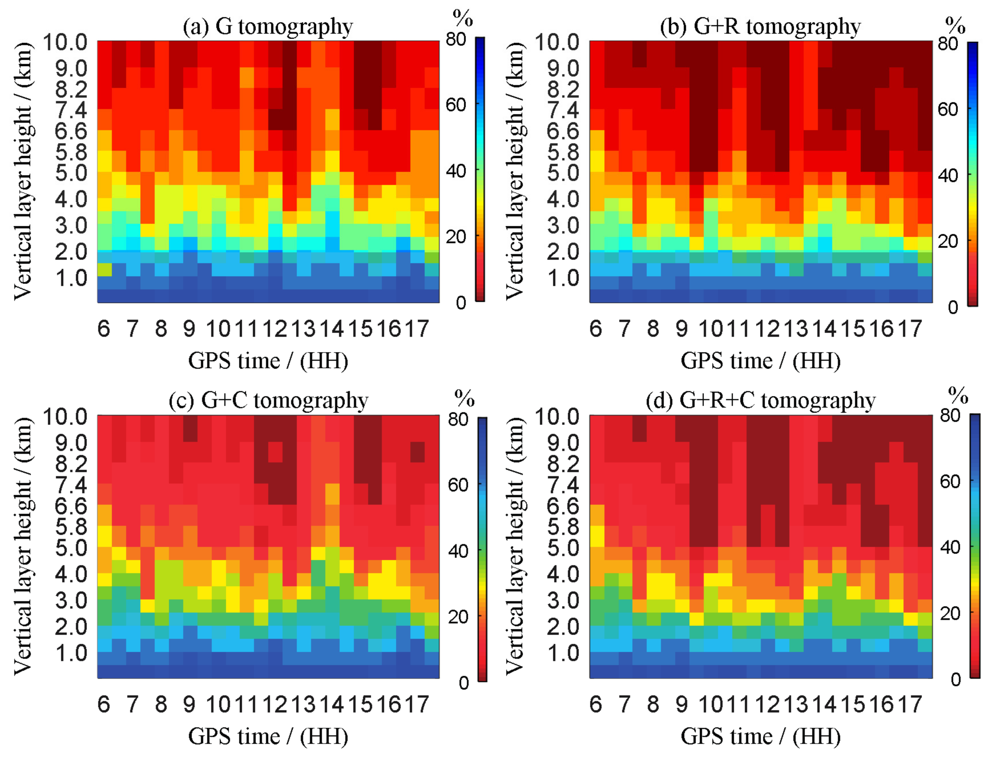
By comparing different GNSS tropospheric tomography results, it can be found that the integrated multi-GNSS systems can significantly increase the number of tomography signals, improve the spatial distribution of inversion signals in tomographic grid, as well as obtain more stable inversed solutions than standalone systems, and multi-GNSS system results are better than standalone ones, which will benefit in the research of weather and climate change. The performances of dual-system tomography and triple-system tomography are almost closed, which means that the additional signals from other GNSS systems added to dual-GNSS tomography have little effect on the final reconstructed water vapor density fields. From the single GPS system to the dual-system, the number of tomographic signals is greatly increased, which generates abounding redundant observations, when the redundant observations achieve a certain extent, and it cannot further improve the accuracy of the tomographic results because these signals cannot increase the number of voxels crossed by signals, especially when located at the bottom. Figure 10 shows the empty rate of voxels at different grid layers in each tomography window from UTC 6:00 to 18:00 on DOY 171, 2014. The average tomographic grid passing rates for different GNSS systems above and below 5 km for seven days are listed in Table 9. In the case of GPS-only tomography, the voxel passing rate is higher above 5 km in the grid. Although the number of GPS + GLONASS signals is increased 1.6 times, the percentage of voxels crossed by signals only improves by 6.3%, and most of the new signals contribute as redundant observations. Since the number of visible satellites in the BDS system is less than GLONASS during the experiment, and given the special distribution of BDS orbits, the empty rate of the GPS + BDS tomographic grid decreased by just 2.2%. The grid empty rate of the GPS + GLONASS + BDS triple-system is reduced by just 0.4% when compared with GPS + GLONASS. Below 5 km, the closer the signal to the GNSS receiver, the denser the distribution of the signals, so the improvement of the empty rate with the integrated multi-GNSS tomography is still limited.
5. Conclusions
In this paper, the multi-GNSS observations provided by the CORS network in Wuhan, China are used to reconstruct 3-D water vapor, and the tomographic results are validated by radiosonde data and the latest ERA5 reanalysis products. The results show that in comparison with the GPS-only system, the average number of effective signals for GPS + GLONASS, GPS + BDS, and GPS + GLONASS + BDS increases 1.6 times, 1.6 times, and 2.2 times, respectively, in each tomographic window for seven days in our experiment, while the corresponding grid passing rate is improved by 5%, 2%, and 6%, respectively. The GNSS tomographic water vapor density profiles have a good agreement with radiosonde data and the ERA5 atmospheric model. The reliability of tomographic water vapor density reconstructed by combining multi-GNSS is significantly enhanced when compared to the GPS-only system with attributing the abundant redundant observations, and inversion accuracy of the GNSS tropospheric tomographic results is improved by 5% from the GPS-only system to the dual-system. The tomographic results are almost similar between the dual-system and the triple-system. However, the number of GNSS signals in the triple-system, or more, increases significantly at the same tomography window, so the combined multi-GNSS systems can improve the temporal resolution of the tropospheric tomography, which has potential to expand applications in the future.
Acknowledgments
The authors would like to thank ECMWF for providing meteorological reanalysis data. This research is supported by the National Natural Science Foundation of China (NSFC) Project (grant no. 11573052).
Author Contributions
Shuanggen Jin and Zhounan Dong conceived and designed the experiments; Zhounan Dong performed the experiments and analyzed the data; and both authors contributed to the writing of the paper.
Conflicts of Interest
The authors declare no conflict of interest.
References
- Bevis, M.; Businger, S.; Herring, T.A.; Rocken, C.; Anthes, R.A.; Ware, R.H. GPS meteorology: Remote sensing of atmospheric water vapor using the Global Positioning System. J. Geophys. Res. Atmos. 1992, 97, 15787–15801. [Google Scholar] [CrossRef]
- Flores, A.; Ruffini, G.; Rius, A. 4D tropospheric tomography using GPS slant wet delays. Ann. Geophys. 2000, 18, 223–234. [Google Scholar] [CrossRef]
- Jin, S.; Li, Z.; Cho, J. Integrated water vapor field and multiscale variations over China from GPS measurements. J. Appl. Meteorol. Climatol. 2008, 47, 3008–3015. [Google Scholar] [CrossRef]
- Jin, S.; Luo, O.F.; Gleason, S. Characterization of diurnal cycles in ZTD from a decade of global GPS observations. J. Geod. 2009, 83, 537–545. [Google Scholar] [CrossRef]
- Jin, S.; Luo, O.F. Variability and climatology of PWV from global 13-year GPS observations. IEEE Trans. Geosci. Remote Sens. 2009, 47, 1918–1924. [Google Scholar]
- Jin, S.; Cardellach, E.; Xie, F. GNSS Remote Sensing: Theory, Methods and Applications; Springer Netherlands: Berlin, Germany, 2014; pp. 48–60. ISBN 978-94-007-7482-7. (eBook). [Google Scholar]
- Guo, J.; Yang, F.; Shi, J.; Xu, C. An Optimal Weighting Method of Global Positioning System (GPS) Troposphere Tomography. IEEE J. Sel. Top. Appl. Earth Observ. 2016, 9, 5880–5887. [Google Scholar] [CrossRef]
- Sá, A.; Bento, F.; Fernandes, R.; Crocker, P. Tomographic determination of the spatial Distribution of Water Vapor using GNSS observations. ALEGG 2016. [Google Scholar] [CrossRef]
- Yao, Y.; Zhao, Q. Maximally Using GPS Observation for Water Vapor Tomography. IEEE Trans. Geosci. Remote Sens. 2016, 54, 7185–7196. [Google Scholar] [CrossRef]
- Guerova, G.; Jones, J.; Dousa, J.; Dick, G.; de Haan, S.; Pottiaux, E.; Bock, O.; Pacione, R.; Elgered, G.; Vedel, H.; et al. Review of the state of the art and future prospects of the ground-based GNSS meteorology in Europe. Atmos. Meas. Tech. 2016, 9, 5385–5406. [Google Scholar] [CrossRef]
- Chen, B.; Liu, Z. Voxel-optimized regional water vapor tomography and comparison with radiosonde and numerical weather model. J. Geod. 2014, 88, 691–703. [Google Scholar] [CrossRef]
- Yao, Y.; Zhao, Q. A novel, optimized approach of voxel division for water vapor tomography. Meteorol. Atmos. Phys. 2017, 129, 57–70. [Google Scholar] [CrossRef]
- Chen, B.; Liu, Z. Assessing the performance of troposphere tomographic modeling using multi-source water vapor data during Hong Kong’s rainy season from May to October 2013. Atmos. Meas. Tech. 2016, 9, 5249–5263. [Google Scholar] [CrossRef]
- Ye, S.; Xia, P.; Cai, C. Optimization of GPS water vapor tomography technique with radiosonde and COSMIC historical data. Ann. Geophys. 2016, 34, 789–799. [Google Scholar] [CrossRef]
- Wang, X.; Wang, X.; Dai, Z.; Ke, F.; Cao, Y.; Wang, F.; Song, L. Tropospheric wet refractivity tomography based on the BeiDou satellite system. Adv. Atmos. Sci. 2014, 31, 355–362. [Google Scholar] [CrossRef]
- Benevides, P.; Nico, G.; Catalão, J.; Miranda, P.M. Analysis of Galileo and GPS Integration for GNSS Tomography. IEEE Trans. Geosci. Remote Sens. 2017, 55, 1936–1943. [Google Scholar] [CrossRef]
- Rohm, W. The ground GNSS tomography–unconstrained approach. Adv. Space Res. 2013, 51, 501–513. [Google Scholar] [CrossRef]
- Davis, J.L.; Elgered, G.; Niell, A.E.; Kuehn, C.E. Ground-based measurement of gradients in the “wet” radio refractivity of air. Radio Sci. 1993, 28, 1003–1018. [Google Scholar] [CrossRef]
- Bender, M.; Dick, G.; Ge, M.; Deng, Z.; Wickert, J.; Kahle, H.G.; Raabe, A.; Tetzlaff, G. Development of a GNSS water vapour tomography system using algebraic reconstruction techniques. Adv. Space Res. 2011, 47, 1704–1720. [Google Scholar] [CrossRef]
- Jin, S.; Park, J.U. GPS ionospheric tomography: A comparison with the IRI-2001 model over South Korea. Earth Planets Space 2007, 59, 287–292. [Google Scholar] [CrossRef]
- Jin, S.; Park, J.U.; Wang, J.L.; Choi, B.K.; Park, P.H. Electron density profiles derived from ground-based GPS observations. J. Navig. 2006, 59, 395–401. [Google Scholar] [CrossRef]
- Notarpietro, R.; Cucca, M.; Gabella, M.; Venuti, G.; Perona, G. Tomographic reconstruction of wet and total refractivity fields from GNSS receiver networks. Adv. Space Res. 2011, 47, 898–912. [Google Scholar] [CrossRef]
- Cai, C.; Gao, Y.; Pan, L.; Zhu, J. Precise point positioning with quad-constellations: GPS, BeiDou, GLONASS and Galileo. Adv. Space Res. 2015, 56, 133–143. [Google Scholar] [CrossRef]
Figure 1.
The principle of GNSS tropospheric water vapor tomography.
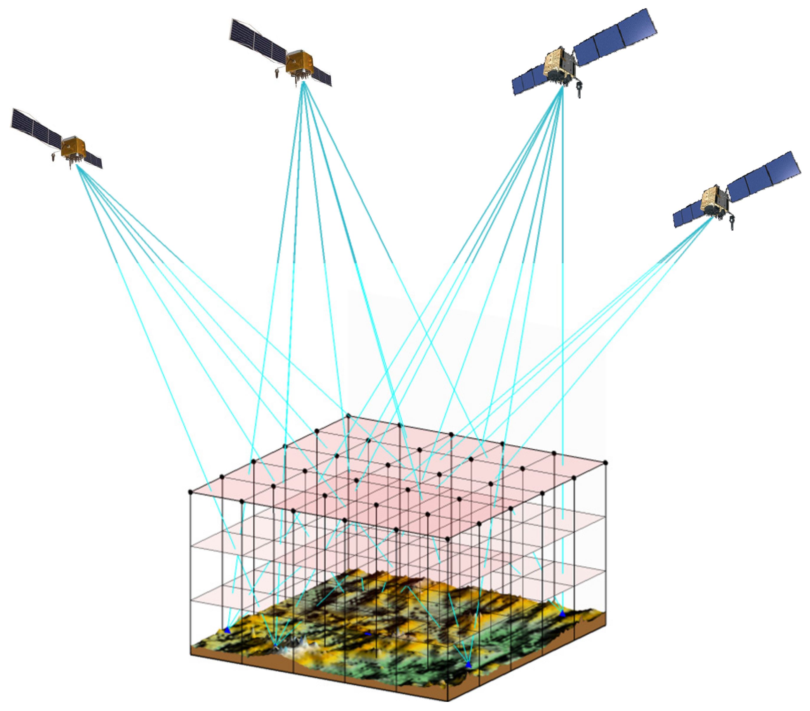
Figure 2.
Average water vapor density and SD from radiosonde station 57,494 from 2004 to 2013.

Figure 3.
The geographic distribution of GNSS stations and radiosonde.
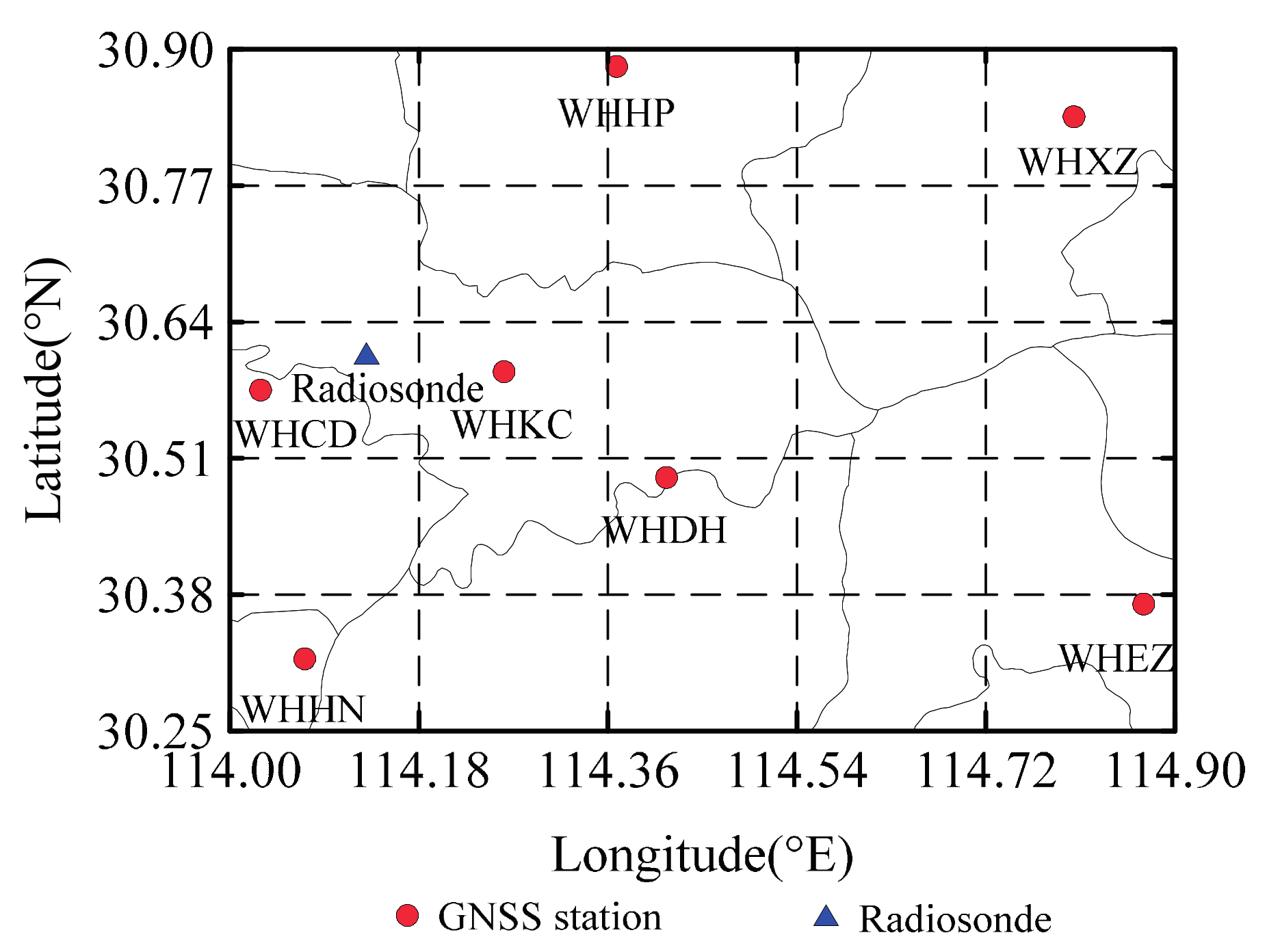
Figure 4.
Effective SWV signals and the percentage of voxels crossed by signals of different GNSS tomography systems in each tomography window from UTC 6:00 to 18:00 on DOY 171, 2014. (a) The number of validated GNSS tomography signals; and (b) the percentage of voxels crossed by the GNSS signals.
Figure 4.
Effective SWV signals and the percentage of voxels crossed by signals of different GNSS tomography systems in each tomography window from UTC 6:00 to 18:00 on DOY 171, 2014. (a) The number of validated GNSS tomography signals; and (b) the percentage of voxels crossed by the GNSS signals.

Figure 5.
(a–g) represent profiles from different combined multi-GNSS systems, radiosonde, and ECMWF at WHCD station at UTC 12:00 from DOY 170 to 176, 2014.
Figure 5.
(a–g) represent profiles from different combined multi-GNSS systems, radiosonde, and ECMWF at WHCD station at UTC 12:00 from DOY 170 to 176, 2014.

Figure 6.
RMS (a) and relative error (b) at different heights of tomography results.
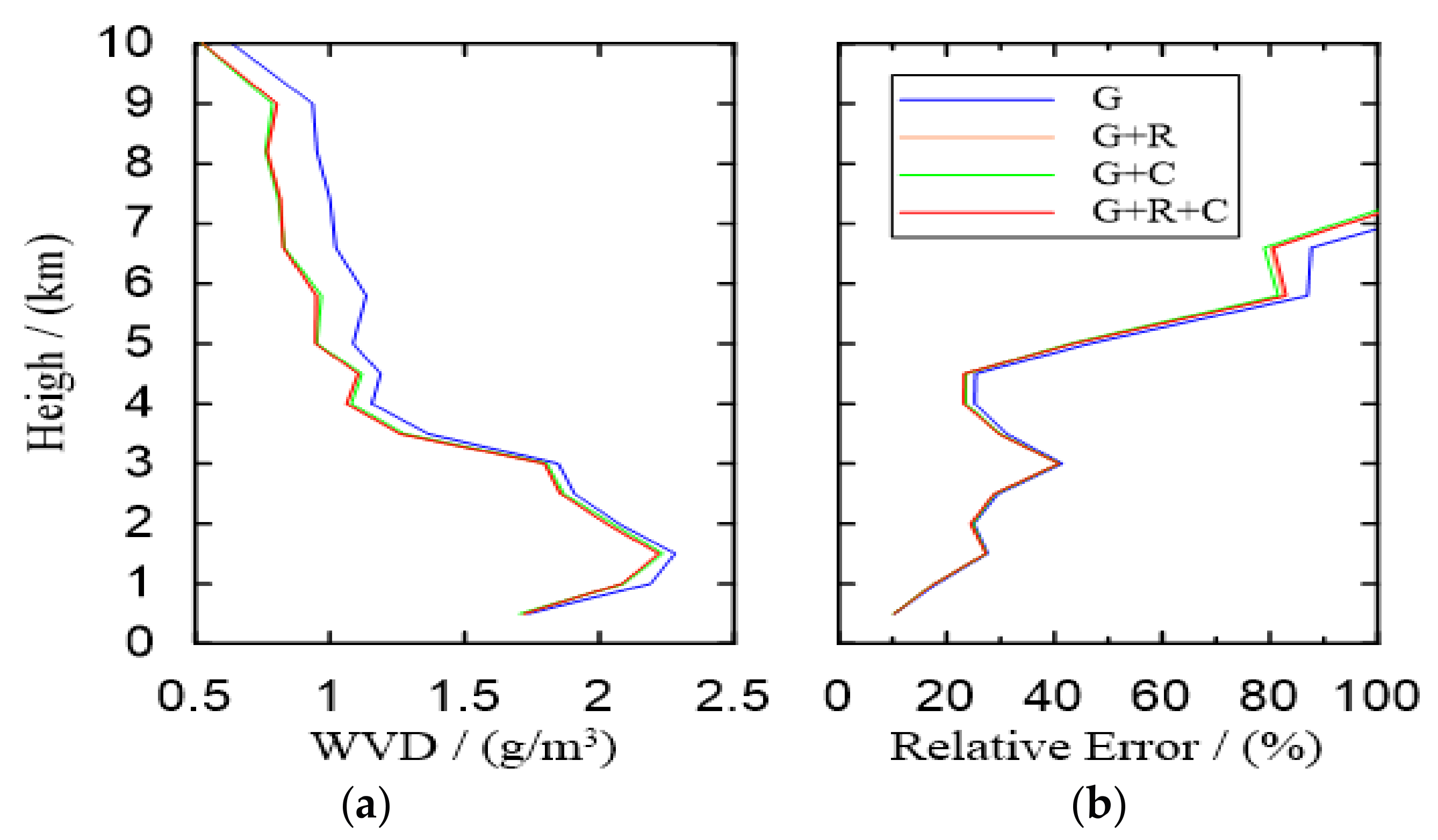
Figure 7.
Linear regression of water vapor density from GNSS tomography and ECMWF. (a–d) represent the regression results of GPS-only, GPS + GLONASS, GPS + GLONASS + BDS, respectively.
Figure 7.
Linear regression of water vapor density from GNSS tomography and ECMWF. (a–d) represent the regression results of GPS-only, GPS + GLONASS, GPS + GLONASS + BDS, respectively.
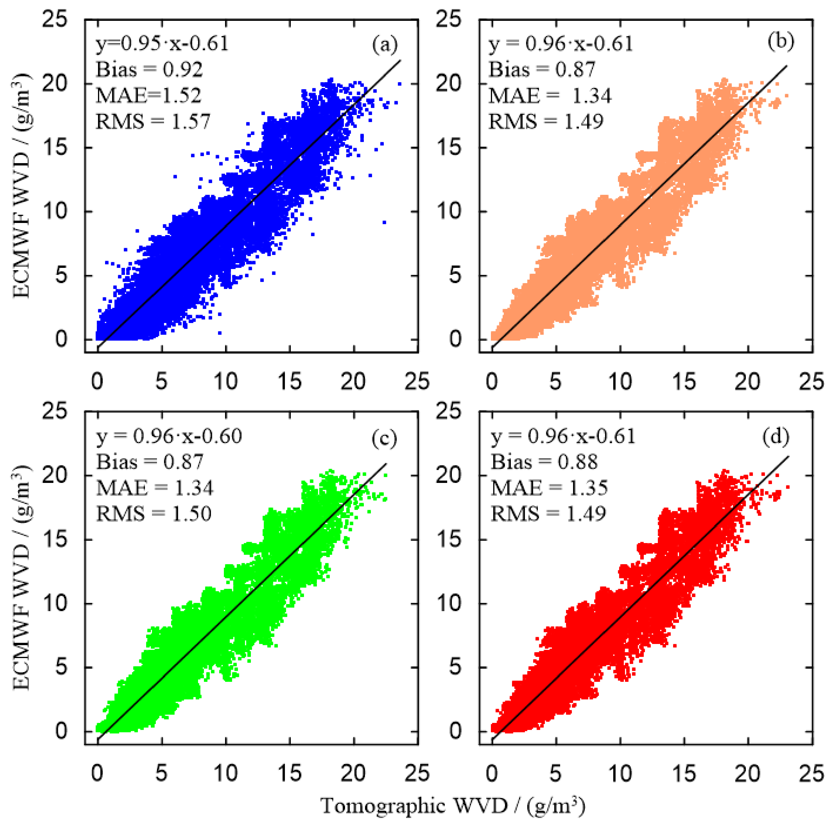
Figure 8.
Comparison of PWV time series at the radiosonde station derived from GNSS tomographic results, raw PWV estimated in the triple-system, ECMWF, and radiosonde.
Figure 8.
Comparison of PWV time series at the radiosonde station derived from GNSS tomographic results, raw PWV estimated in the triple-system, ECMWF, and radiosonde.

Figure 9.
Residual distributions of different combined-GNSS tomography results.
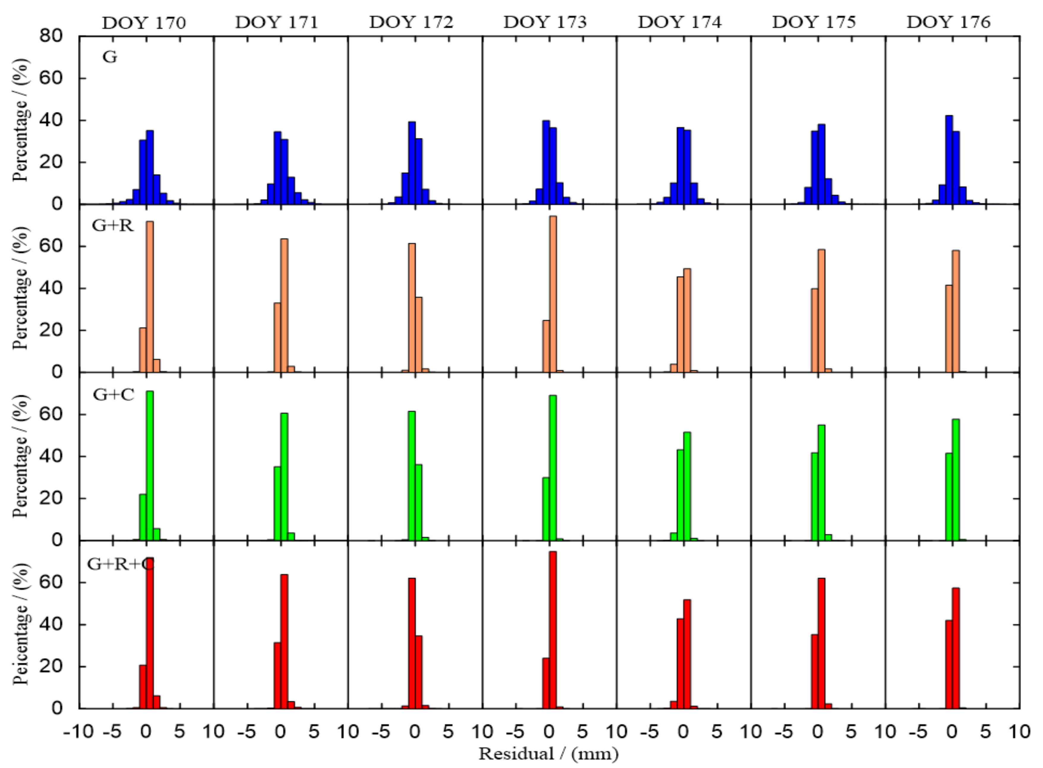
Figure 10.
The percentage of empty voxels with different combined GNSS in different layers.


Table 1.
GNSS station information and weather conditions during the experiment for seven days.
| Station Location | Weather Conditions | |||||
|---|---|---|---|---|---|---|
| Station | Latitude | Longitude | Height | DOY | Weather | Wind Direction |
| WHCD | 30°34′31″ | 114°1′44″ | 36.9 | 170 | light rain turns to moderate rain | north |
| WHDH | 30°29′31″ | 114°24′56″ | 45.7 | 171 | overcast to cloudy | north |
| WHEZ | 30°22′16″ | 114°52′13″ | 60.2 | 172 | overcast to cloudy | north |
| WHHN | 30°19′8″ | 114°4′16″ | 57.4 | 173 | cloudy | north |
| WHHP | 30°53′2″ | 114°22′5″ | 34.1 | 174 | cloudy | northwest |
| WHKC | 30°35′34″ | 114°15′39″ | 45.9 | 175 | light rain turns to moderate rain | northeast |
| WHXZ | 30°50′9″ | 114°48′13″ | 40.9 | 176 | heavy rain turns to moderate rain | east |
Table 2.
Statistics of Pearson correlation between tomography profiles and ERA5 profiles.
| SYS | G | G + R | G + C | G + R + C |
|---|---|---|---|---|
| Mean Person correlation | 95.90% | 96.40% | 96.40% | 96.40% |
Table 3.
Statistical results of GNSS tomographic water vapor density below 5 km (unit: g/m3).
| DOY | MAE | RMS | ||||||
|---|---|---|---|---|---|---|---|---|
| G | G + R | G + C | G + R + C | G | G + R | G + C | G + R + C | |
| 170 | 0.98 | 0.85 | 0.82 | 0.86 | 1.14 | 0.94 | 0.94 | 0.94 |
| 171 | 1.45 | 1.35 | 1.33 | 1.35 | 1.66 | 1.50 | 1.50 | 1.50 |
| 172 | 1.39 | 1.33 | 1.35 | 1.33 | 1.39 | 1.32 | 1.33 | 1.32 |
| 173 | 1.36 | 1.26 | 1.26 | 1.27 | 1.51 | 1.47 | 1.47 | 1.47 |
| 174 | 1.17 | 1.12 | 1.17 | 1.12 | 1.32 | 1.28 | 1.27 | 1.29 |
| 175 | 1.62 | 1.57 | 1.57 | 1.57 | 1.78 | 1.72 | 1.72 | 1.72 |
| 176 | 1.95 | 1.91 | 1.91 | 1.92 | 1.94 | 1.86 | 1.87 | 1.87 |
Table 4.
Statistical result of GNSS tomographic water vapor density below 5 km for seven days (unit: g/m3).
Table 4.
Statistical result of GNSS tomographic water vapor density below 5 km for seven days (unit: g/m3).
| SYS | G | G + R | G + C | G + R + C |
|---|---|---|---|---|
| Bias | 0.77 | 0.74 | 0.74 | 0.75 |
| MAE | 1.54 | 1.48 | 1.49 | 1.48 |
| RMS | 1.82 | 1.76 | 1.77 | 1.76 |
Table 5.
Statistical result of PWV differences between GNSS tomography and ECMWF at the radiosonde station (unit: mm).
Table 5.
Statistical result of PWV differences between GNSS tomography and ECMWF at the radiosonde station (unit: mm).
| SYS | Bias | RMS | Maximum |
|---|---|---|---|
| G | 5.32 | 3.06 | 10.23 |
| G + R | 4.42 | 2.84 | 10.98 |
| G + C | 4.58 | 2.95 | 12.86 |
| G + R + C | 4.49 | 2.83 | 11.02 |
Table 6.
Statistical result of PWV differences between GNSS tomography and ECMWF at all stations for seven days (unit: mm).
Table 6.
Statistical result of PWV differences between GNSS tomography and ECMWF at all stations for seven days (unit: mm).
| SYS | Bias | RMS | Maximum |
|---|---|---|---|
| G | 4.59 | 3.72 | 15.20 |
| G + R | 3.66 | 3.52 | 13.07 |
| G + C | 3.94 | 3.73 | 14.96 |
| G + R + C | 3.68 | 3.50 | 12.84 |
Table 7.
Comparison of tomography residuals between different combined GNSS systems for seven days (unit: mm).
Table 7.
Comparison of tomography residuals between different combined GNSS systems for seven days (unit: mm).
| DOY | MAE | RMS | ||||||
|---|---|---|---|---|---|---|---|---|
| G | G + R | G + C | G + R + C | G | G + R | G + C | G + R + C | |
| 170 | 0.97 | 0.36 | 0.33 | 0.36 | 1.45 | 0.43 | 0.44 | 0.45 |
| 171 | 0.94 | 0.27 | 0.27 | 0.30 | 1.30 | 0.37 | 0.40 | 0.43 |
| 172 | 0.79 | 0.25 | 0.23 | 0.26 | 1.06 | 0.37 | 0.34 | 0.39 |
| 173 | 0.69 | 0.20 | 0.18 | 0.21 | 0.99 | 0.26 | 0.25 | 0.26 |
| 174 | 0.77 | 0.31 | 0.30 | 0.31 | 1.09 | 0.46 | 0.45 | 0.47 |
| 175 | 0.75 | 0.19 | 0.20 | 0.20 | 1.05 | 0.29 | 0.32 | 0.31 |
| 176 | 0.68 | 0.16 | 0.17 | 0.17 | 1.00 | 0.24 | 0.24 | 0.24 |
Table 8.
Statistical result of different GNSS tomography systems for seven days (unit: mm).
| SYS | G | G + R | G + C | G + R + C |
|---|---|---|---|---|
| MAE | 0.80 | 0.25 | 0.24 | 0.26 |
| RMS | 1.15 | 0.37 | 0.37 | 0.39 |
Table 9.
The percentage of empty voxels below and above 5 km.
| SYS | G | G + R | G + C | G + R + C |
|---|---|---|---|---|
| 5 km below | 45.30% | 40.30% | 44.10% | 39.90% |
| 5 km above | 12.60% | 6.30% | 10.40% | 5.80% |
© 2018 by the authors. Licensee MDPI, Basel, Switzerland. This article is an open access article distributed under the terms and conditions of the Creative Commons Attribution (CC BY) license (http://creativecommons.org/licenses/by/4.0/).
Share and Cite
MDPI and ACS Style
Dong, Z.; Jin, S. 3-D Water Vapor Tomography in Wuhan from GPS, BDS and GLONASS Observations. Remote Sens. 2018, 10, 62. https://doi.org/10.3390/rs10010062
AMA Style
Dong Z, Jin S. 3-D Water Vapor Tomography in Wuhan from GPS, BDS and GLONASS Observations. Remote Sensing. 2018; 10(1):62. https://doi.org/10.3390/rs10010062
Chicago/Turabian StyleDong, Zhounan, and Shuanggen Jin. 2018. "3-D Water Vapor Tomography in Wuhan from GPS, BDS and GLONASS Observations" Remote Sensing 10, no. 1: 62. https://doi.org/10.3390/rs10010062
Note that from the first issue of 2016, this journal uses article numbers instead of page numbers. See further details here.