Using a MODIS Index to Quantify MODIS-AVHRRs Spectral Differences in the Visible Band


1
Key Laboratory of Watershed Geographic Sciences, Chinese Academy of Sciences, Nanjing 210008, China
2
Nanjing Institute of Geography and Limnology, Chinese Academy of Sciences, Nanjing 210008, China
*
Author to whom correspondence should be addressed.
Remote Sens. 2018, 10(1), 61; https://doi.org/10.3390/rs10010061
Submission received: 6 November 2017
/
Revised: 23 December 2017
/
Accepted: 3 January 2018
/
Published: 4 January 2018
(This article belongs to the Special Issue Analysis of Multi-temporal Remote Sensing Images)
Abstract
:Spectral band differences are a critical issue for progressing into an integrated earth observation framework and in particular, in sensor intercalibration. The differences are currently normalized using spectral band adjustment factor (SBAF) that is generated from hyperspectral data. In this context, the current study proposes a method for calculating moderate-resolution imaging spectroradiometer (MODIS)-advanced very high resolution radiometers (AVHRRs) SBAF in the visible band, using the MODIS surface reflectance data. The method involves a uniform ratio index calculated using the MODIS 552-nm and 645-nm bands, and a sensor-specific quadratic equation, producing SBAF data at 500-m spatial resolution. The calculated SBAFs are in good agreement at site scale with literature reported data (relative error < 1.0%), and at local scale with Hyperion-derived data (total uncertainty ≈ 0.001), and significantly improve MODIS-AVHRR surface reflectance data consistency in the visible band (better than 1.0% reflectance units). The calculation is more sensitive to atmospheric effects over the vegetated areas. At global scale, MODIS-AVHRRs SBAFs are generally large (>1.0) over densely vegetated areas and extremely low over deserts and barren lands (0.96–0.98), indicative of large MODIS-AVHRRs differences. Deserts show temporally stable SBAF values, while still suffer from intra-annual BRDF effects and short-term cloud contamination. By means of daily MODIS data, the proposed method can produce ongoing SBAF data at a spatial scale that is comparable to AVHRRs. It increases the sampling of MODIS-AVHRRs image pairs for intercalibration, and offers insight into spectral band conversion, finally contributing to an integrated earth observation at moderate spatial resolutions.
1. Introduction
The need for integrated earth observation framework has been highly recognized by science community, and promoted by space agencies [1,2]. Integration of various satellite data generally extends the length of data series [3,4] and improves spatiotemporal resolutions of the individual data [5,6], providing enhanced capabilities to resolve land surface processes and changes. At ten-meter spatial resolutions, the Landsat MSS (multispectral scanner)/TM (thematic mapper)/ETM+ (enhanced thematic mapper plus)/OLI (operational land imager) and Sentinel-2 Multispectral Instrument (MSI) observe the earth within ten days, gaining spatially well-resolved information on ecological and other issues at regional scales [7]. With almost the same historical span, the advanced very high resolution radiometers (AVHRRs) provide decades of daily observations. The high frequency leads to increased probability of cloud free observations, and via composting method yields near-seamless data records in support of global change studies [3,8,9]. However, AVHRRs lack onboard calibration devices in the reflective solar bands, which may significantly reduce the value for quantitative studies. Determination of sensor calibration coefficients often relies on vicarious calibration, cross-calibration (as intercalibration in [10]) and pseudo-invariant calibration, of which the intercalibration method has been widely used for AVHRRs calibration [11].
The lessons from AVHRRs are learnt and advantages are inherited by two follow-on moderate-resolution imaging spectroradiometer (MODIS) sensors onboard Terra (since 1999) and Aqua (since 2002) platforms. Specifically, the two sensors have onboard accurate and stable calibrators [12]. The calibrated radiance data (±2% uncertainty) and the derived surface reflectance data (±5% uncertainty) provide ideal references for MODIS-AVHRRs intercalibration [13]. The former offer high radiometric standard that is transferrable to AVHRRs, and the latter characterize the surface condition and long-term stability of calibration sites [14,15]. For MODIS-AVHRRs intercalibration, however, the excellent radiometric accuracy can be compromised by, if not corrected, the spectral band differences. Due to both technical advancement and practical considerations, MODIS and AVHRRs are deployed with spectrally similar but not identical bands [16], which might cause inconsistencies among multisensor data [17] and pose challenges to MODIS-AVHRRs intercalibration [13]. Recently, Fan and Liu [18] propose a general intercalibration method for the MODIS-AVHRRs visible bands over homogeneous land surfaces. The two-step method requires corrections of spectral band differences and atmospheric effects, contributing to increased sampling of MODIS-AVHRRs reflectance pairs and therefore robust calibration results. Over these homogeneous land surfaces, especially the desert sites, normalization between MODIS-AVHRRs reflectances is critical [14,19,20].
Normalization here refers to the process that removes variations in satellite observations due to spectral band differences. The differences are previously addressed in terms of spectral band width and positioning [21], and currently in terms of spectral response function (SRF). The effect is defined as spectral band difference effect (SBDE) [22], which may impact on sensor intercalibration and climate data record generation [23,24]. Traditionally, it is adjusted using intersensor transformation equations [25,26]. In most cases, the spectral measurements [27], spectral library data [28] and multi-/hyper-spectral images [29,30] are used to derive these equations. Moreover, radiative transfer models are used to predict at-sensor reflectances based on surface reflectances and atmospheric conditions [31]. Spectral band adjustment factor (SBAF) is used [32] to adjust spectral band differences for sensor intercalibration. Initially, Chander et al. [33] propose a figure-of-merit index, which is defined as SRFs intersection/union ratio. Similar index can be found in [34] using two fictitious SRFs. Aside from SRFs, more studies address the SBAF dependence on scene content. Teillet et al. [22] and Li et al. [35] show more SBAF dependence on surface condition than atmospheric condition and observational geometry. Teillet et al. [36] state that atmospheric absorption is the main source of SBAF variations for the same underlying surface. Similarly, Wu et al. [37] investigate SBAF sensitivities in particular to water vapor. For the bidirectional reflectance distribution function (BRDF) effects, Wang et al. [38] demonstrate the suitability of nadir reflectances for SBAF calculation, when sensors share the same sun–target–sensor geometries. Overall, SRFs and scene content are both important to calculate SBAF.
SBAFs are calculated from multispectral data, using spectral interpolation methods. Teillet et al. [39] initially obtain continuous reflectance profiles from Landsat TM spectral band reflectances using linear interpolation, and then derive AVHRR spectral band reflectances. Similarly, Röder et al. [40] compare and determine the optimal interpolation method for converting Landsat TM to MSS spectral band radiances. To improve the accuracy of spectral interpolation, Henry et al. [41] use multisensor data to fit reflectance profiles. Moreover, Feng et al. [42] and Li et al. [43] obtain SBAFs via a matching procedure between remote sensing reflectance data and the United States Geological Survey (USGS) spectral library data. Relative to methods that use multispectral data, however, hyperspectral data are more appreciated for their fine spectral resolutions [44,45]. Currently, the Earth Observing One (EO-1) Hyperion and the ENVISAT Scanning Imaging Absorption Spectrometer for Atmospheric Chartography (SCIAMACHY) are the main hyperspectral sensors used for calculating SBAFs [32,45]. Both sensors have their advantages and disadvantages. The Hyperion has a spatial resolution of 30 m, which can provide spatially detailed SBAF data. However, it has a swath width of only 7.5 km, and the number of available images is limited, which is insufficient for frequent SBAF updating. The SCIAMACHY has the ability of global coverage. However, it has a spatial resolution of 60 km × 30 km, much coarser than MODIS and AVHRRs. From the perspective of sensor intercalibration, both data may be qualified over large homogenous calibration sites. That is, the narrow Hyperion scene is representative of the whole site, and the coarse SCIAMACHY pixel bears subpixel homogeneity. However, small sites might suffer from insufficient temporal coverage of Hyperion and coarse spatial resolution of SCIAMACHY. It is favorable to obtain SBAF data at spatial scales comparable to MODIS and AVHRRs, in order for their intercalibration.
The objective of this study is to propose an SBAF calculation method for normalizing AVHRRs and MODIS visible band surface reflectances, in an initial effort to improve sensor calibration and a further implication for multisensor data consistency. Initially, the reference MODIS-AVHRRs SBAFs are calculated and correlated with normalized difference reflectance indices, supported by spectral library data. Then, the optimal index is determined and reshaped using MODIS spectral bands, which are also simulated from spectral library data. Statistical regressions are performed between the reference SBAFs and the MODIS index for sensor specific SBAF calculation equations. The derived SBAFs are comprehensively validated at site and local scales, and analyzed for spatial and temporal variations. The proposed method would create more AVHRRs-MODIS intercalibration opportunities, and provide a valuable insight into creating multisensor data consistency.
2. Materials and Methods
2.1. Instruments Overview and SBAF Calculation
AVHRRs are deployed on the National Oceanic and Atmospheric Administration (NOAA) and MetOp-A(B) platforms. In this study, the instruments include AVHRR/1 aboard NOAA-8/10, AVHRR/2 aboard NOAA-7/9/11/12/14, AVHRR/3 sensors aboard NOAA-15~19 and MetOp-A, and MODIS/Terra. Figure 1 shows the SRFs in the visible band. The AVHRR SRFs are spectrally wider than the MODIS SRF. SRFs are narrower for AVHRR/3 than AVHRR/1-2. All SRF data were resampled to 1 nm (350~2400 nm) and used to calculate SBAFs [33]:
where ρ denotes reflectance profile, λ denotes wavelength, and SRF denotes spectral response function in Figure 1.
2.2. Deriving the Index and Equations for SBAF Calculation
SBAFs were calculated using a uniform index and sensor specific equation for each AVHRR. The index was derived based on the USGS spectral library (splib06) data. With over 1300 spectra records [46], the library offers an ideal data resource for multipurpose studies, including SBAF determination [41]. Initially, the data were screened by flags ‘0.000000’ (not measured) and ‘−1.23 × 1034’ (deleted number). The survived spectra were resampled to 1 nm (350~2400 nm), and calculated for normalized difference reflectance indices (NDRI) using
where λi, λj (i > j) denote two different spectral wavelengths.
To match the spectra data, MODIS and AVHRRs SRFs were also resampled to 1 nm. Then SBAFs were calculated using Equation (1), and used as reference data for model development. Subsequently, the Pearson’s correlation coefficients (r) were calculated between the reference SBAF and NDRIs for each MODIS-AVHRR pair. The NDRI with the maximum averaged r value (over all MODIS-AVHRR pairs) was selected as the optimal index (NDRI0). Finally, the compositional bands in NDRI0 were estimated from neighboring MODIS bands using the method in [47]:
where λ0 denotes each band of NDRI0, MOD1 and MOD2 are two neighboring MODIS bands (MOD1 < λ0 < MOD2), and l1, l2 are regression coefficients.
The reflectances in the MOD1 and MOD2 bands were calculated by convolving the USGS spectra data with the corresponding MODIS SRFs. The reflectance in the λ0 band was extracted directly from the USGS spectra data. Then, the coefficients l1, l2 were determined using a multiple linear regression. Similarly, both bands in NDRI0 were reshaped using MODIS bands, and NDRI0 was then transformed to a MODIS index. For each AVHRR, a quadratic equation was determined between the reference SBAF and the uniform MODIS index, which was used for SBAF calculation. The equation for SBAF calculation is written as
where MOD_Ind denotes the MODIS index, a0, a1 and a2 are sensor specific regression coefficients.
2.3. Validating the MODIS Based Method
Validations were performed by comparison to the literature reported data (site scale) and the Hyperion-derived data (local scale). For both validations, the equation in Equation (4) and the required sensor specific coefficients were applied to daily MODIS/Terra Collection 006 (C006) 500-m surface reflectance data (MOD09). At site level, the calculated SBAFs were compared to the data used in sensor intercalibration studies. These data are generally accurate for a reliable sensor intercalibration. Such studies include the NOAA-16 AVHRR vs. MODIS intercalibration over the Saharan desert site in Niger (21.5°N, 14.4°E) on 13 July 2002 [13], the NOAA-17 AVHRR vs. MODIS intercalibration over the Dunhuang Gobi site (40.2°N, 94.4°E) on 7 November 2002 [48]. Both sites belong to the Committee on Earth Observation Satellites (CEOS) endorsed radiometric sites. Besides, SBAF data were available for the NOAA-16/17/18 AVHRR vs. MODIS intercalibration over the Badain Jaran desert site (39.9°N, 101.9°E) on 13 July 2012 [14]. For each site, the required MODIS surface reflectances were extracted from daily MOD09 dataset, and calculated for SBAFs using Equation (4). Relative difference against the literature reported data was calculated to show the errors. Note that these calibration sites are large and spatially homogenous, and the errors due to scale differences (point data vs. 500-m MODIS data) are minimized.
At local scale, the calculated SBAFs were compared to those derived from Hyperion surface reactance data. Hyperion has been validated for SBAF calculations [32]. Two scenes covering the Libya-4 desert site centered at 29.0°N, 23.8°E were collected on 30 April and 16 May 2015, representing nonvegetated areas. Each scene was atmospherically corrected using the fast line-of-sight atmospheric analysis of spectral hypercubes (FLAASH), with the middle-latitude summer atmosphere model. Two scenes were used to test the method stability, because the CEOS endorsed Libya-4 desert site was well-known as spectrally stable over time. This area was selected due to the rich data previously reserved for sensor calibration. Another scene covering the Yellow River Delta, China centered at 37.7°N, 118.8°E was collected on 14 April 2005. It represents the vegetated area and has been well-corrected for atmospheric effects (see [49]). Then, all Hyperion surface reflectance data were calculated for NOAA-19 AVHRR vs. MODIS SBAFs using Equation (1). The ~10-nm Hyperion data were initially resampled to 1-nm, and then convolved using the NOAA-19 AVHRR and MODIS visible band SRFs. The ratios of AVHRR-convolved over MODIS-convolved reflectances provided the reference SBAFs. Meanwhile, the 500-m MODIS/Terra surface reflectances were collected and calculated for SBAFs using Equation (4). Prior to comparison, both SBAF data were aggregated to 1500 m (3 × 3 MODIS pixels, 50 × 50 Hyperion pixels), in order to reduce the effects due to spatial mismatch. The metrics R2 (coefficient of determination) and RMSE (root-mean-square error) were used for evaluation.
2.4. Simulating SBAF Sensitivities to Atmospheric Parameters
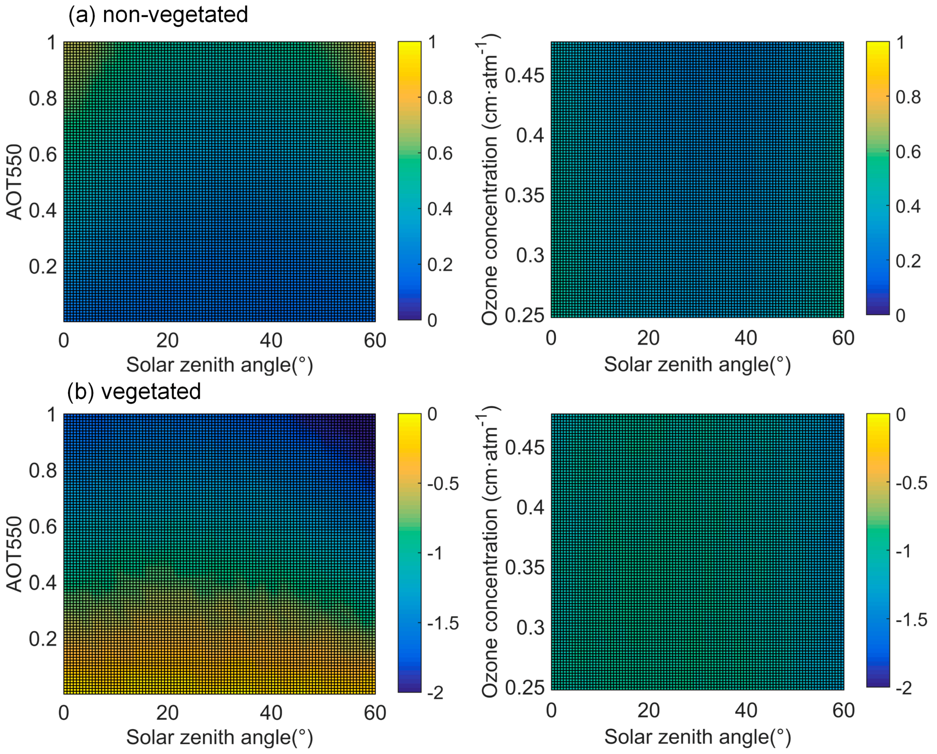
The atmospheric effects are critical, because SBAFs are calculated using surface reflectance data in this study. Here, the NOAA-19 AVHRR was taken to simulate SBAF sensitivities to the total ozone concentration (TOC) and aerosol optical thickness (AOT). Two typical ground objects were selected. One was desert (nonvegetated) with surface reflectance data in [13], and the other was vegetation with surface reflectance data in the USGS spectral library. Then, top-of-atmosphere (TOA) reflectances at the required MODIS bands were simulated under various atmospheric conditions using the Second Simulation of the Satellite Signal in the Solar Spectrum (6S) radiative transfer code [50]. For 6S calculations, the desert and continental aerosol models were specified, respectively, for the two sites. The other atmospheric parameters included TOC = 0.247–0.480 cm·atm−1 [51], AOT = 0–1, solar zenith angle (SZA) = 0–60°, and water vapor content = 1.0 g·cm−2. The AOT range covers the clear to turbid atmospheric conditions, and the SZA range covers the short to long paths for radiative transfer. Because water vapor absorption is weak in the visible bands, the water vapor content was fixed as an arbitrary moderate value. The primary objective of the sensitivity analyses was to investigate the different behaviors of atmospheric effects on SBAF calculation over vegetated and nonvegetated sites. Therefore, both sensors were simplified as nadir-looking for simplification. With TOA reflectances, SBAFs were calculated and compared to those calculated using surface reflectances. Relative differences (TOA level against surface level) were calculated to show the sensitivities of SBAFs to TOC and AOT. The simulations only provide a synoptic view of atmospheric effects, and the actual differences between TOA level and surface level SBAFs can be calculated with auxiliary atmospheric data and sun–target–sensor geometries.
2.5. Investigating Spatiotemporal Patterns of SBAF
Global SBAFs were calculated using the MODIS combined Terra and Aqua 16-day black sky albedo dataset (MCD43C3), and analyzed for their spatial and temporal patterns. The MCD43C3 is generated using MODIS surface reflectance data within a 16-day moving window, and provided as daily 0.05° Climate Modelling Grid (CMG) product. The required surface reflectances were extracted from MCD43C3 and calculated for SBAFs using Equation (4). Here, the data at middle 2016 (DOY183) were used to calculate global NOAA-16~19 AVHRR vs. MODIS SBAFs. Spatially, large MODIS-AVHRR differences should be associated with SBAFs that deviate more from unity. Besides, the recent 5 years (2012–2016) of MCD43C3 albedo data were calculated for NOAA-19 AVHRR vs. MODIS SBAFs. The SBAF time series was inspected at several stable desert sites, including the CEOS endorsed Algeria-3 site (30.32°N, 7.66°E), Arabia-1 site (18.88°N, 46.76°E), Libya-4 site, Mali-1 site (19.12°N, 4.85°W), Taklimakan site (39.83°N, 80.17°E) and the Badain Jaran desert site. Time-invariant SBAFs are favorable for sensor intercalibrations, especially when simultaneous ground observations are lacking.
2.6. Application Examples with MODIS and AVHRR Observations
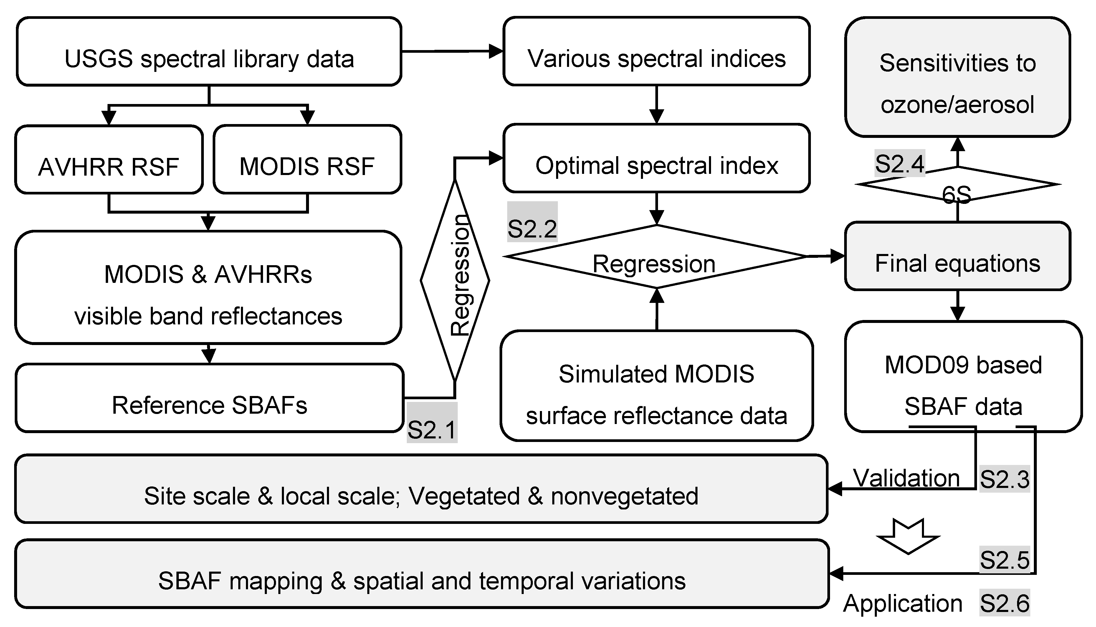
The above analyses are based on MODIS surface reflectances and MODIS/AVHRR SRFs. It is necessary to apply the method to MODIS and AVHRR observations. For this purpose, simultaneously overpassed Terra MODIS and NOAA-17 AVHRR L1B images were collected, and the SBAFs were calculated using the corresponding MODIS surface reflectance data. The images covered low-to-moderate reflective surfaces near the Dunhuang site in DOY116, 2004, and moderate-to-high reflective surfaces near the Libya-4 site in DOY113, 2004 (Figure 2). The pixels with nadir-looking (<10°) sensor view angles were retained, which ensured weak BRDF effects caused by differing MODIS-AVHRR sun–target–sensor geometries. Because sensors overpassed within minutes, the MODIS atmospheric products were used to derive both MODIS and AVHRR visible band surface reflectances. The main data processing steps included (1) performing spatial coregistration using the pixel shifting method [52]; (2) resampling all cloud free data into 0.2° grids to mitigate the effects of residual spatial misregistration; (3) applying radiometric correction to AVHRR images using the revised calibration coefficients; (4) deriving MODIS and AVHRR surface reflectances using the 6S radiative transfer code (desert aerosol model), supported by MODIS atmospheric products and MODIS/AVHRR sun–target–sensor geometry data; and (5) calculating SBAFs using MODIS surface reflectance product. The SBAF data were used to account for the differences between MODIS and AVHRR surface reflectances. The performance of SBAF correction was then evaluated through comparison of MODIS-AVHRR surface reflectances before and after the correction. To clarify all the above-mentioned methods and steps, a flowchart is given in Figure 3.
3. Results
3.1. Equations for Calculating AVHRR-MODIS SBAFs
With the USGS spectra-derived SBAF and NDRIs, the optimal NDRI is determined as composed of the 645-nm and 600-nm bands. The 645-nm band is similar to the MODIS 645-nm band (620–670 nm), and the 600-nm band is then estimated using the MODIS 645-nm (620–670 nm) and 552-nm (545–565 nm) bands. As a result, the uniform MODIS index for SBAF calculation is determined as
where R645 and R552 are surface reflectances at the MODIS 645-nm (620–670 nm) and 552-nm (545–565 nm) bands. The USGS spectra-derived SBAF and the MODIS index are then used to determine SBAF calculation equation for each MODIS-AVHRR pair via quadratic regression method. Table 1 shows the sensor specific equations of SBAF (y) and the MODIS index (MOD_Ind). SBAFs are estimated with R2 = 0.381–0.840 (0.683 ± 0.145) and RMSE = 0.010–0.034 (0.019 ± 0.008). The method performs better for modern sensors (AVHRR/3) than historical sensors (AVHRR/1-2). The R2 values are 0.736–0.769 (0.748 ± 0.012), and the RMSE values are 0.010–0.014 (0.012 ± 0.002) for AVHRR/3, which starts from NOAA-15 through NOAA-19.
3.2. Validation Results of the Calculation Method
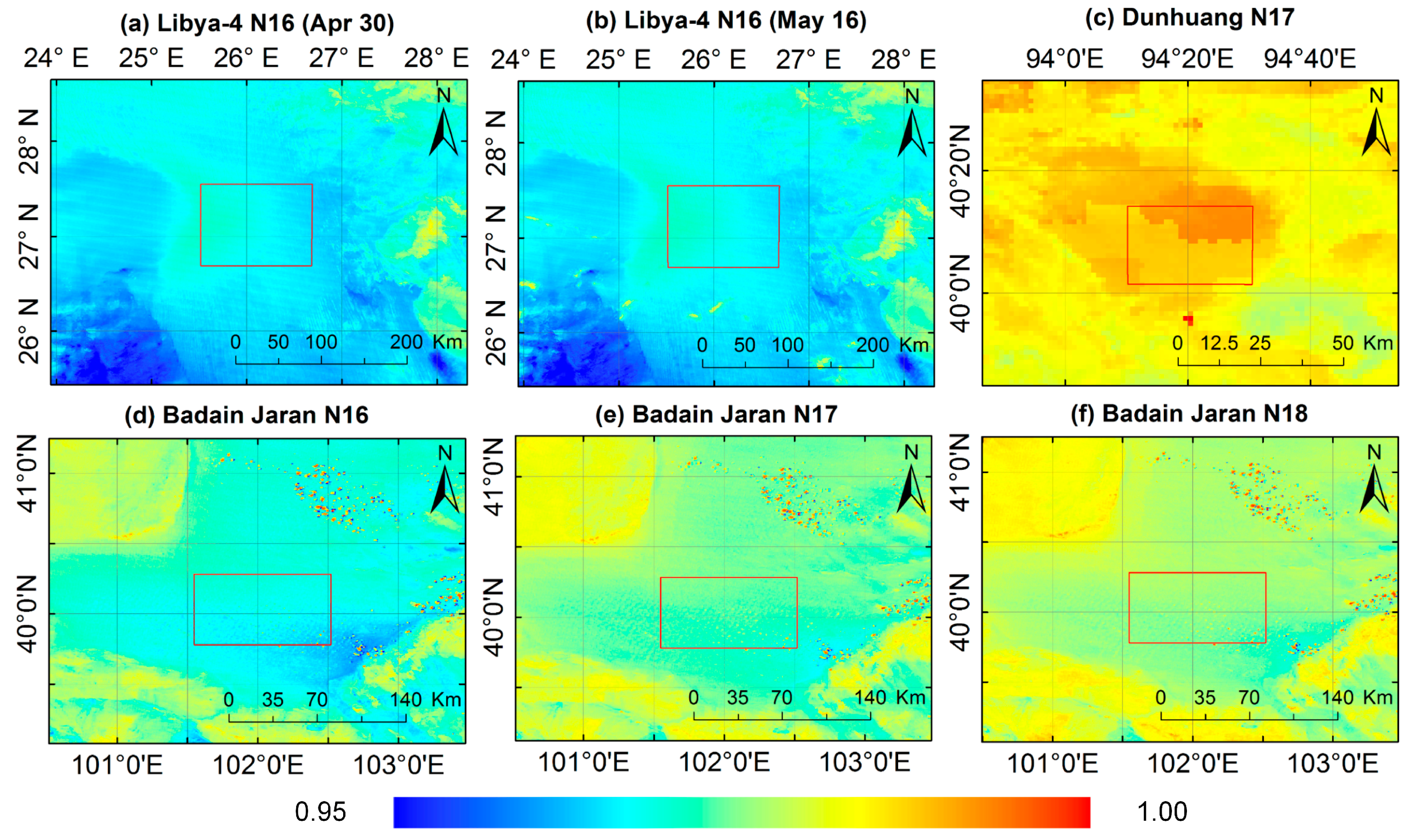
Sensor intercalibration is generally performed at stable calibration sites where surface conditions are generally well-characterized. SBAFs are calculated around these calibration sites and illustrated in Figure 4. The boundaries defined by the red frames are the core calibration sites recommended by the CEOS or the researchers on sensor intercalibration, and the centered data are used for site scale SBAF validation. These sites generally exhibit uniform SBAFs, except for the Dunhuang Gobi site that shows SBAF variations in the north-south direction. Comparison of the calculated and the literature reported SBAF data is shown in Table 2. The relative differences are well within 1%, except for the Niger desert site with a relative difference of 1.2%. Note that the reference SBAF over the Niger desert site is calculated using linearly interpolated MODIS surface reflectance data, while the other SBAFs are calculated using in situ spectral measurements. The relatively large difference might result from inaccurate reflectance profile data. Overall, the site scale validation shows an SBAF calculation error within 1%.
Hyperion data possess well-resolved spectral information that is critical for SBAF calculation. The comparisons between Hyperion-derived and MODIS calculated SBAFs in the case of NOAA-19 AVHRR vs. MODIS are shown in Figure 5. For the Libya-4 site on 30 April (Figure 5a) and 16 May (Figure 5b), the Hyperion-derived SBAFs are concentrated within 0.973–0.980, indicating that the Libya-4 core site and the surrounding areas are homogeneous and suitable for sensor intercalibration. Linear regression between the Hyperion-derived (x) and MODIS calculated (y) SBAFs shows that the R2 (RMSE) values are 0.615 (0.001) and 0.757 (0.001), respectively, on 30 April and 16 May 2015. For the vegetated area, SBAFs exhibit a wide dynamic range and show more scatter in the higher end of SBAF (Figure 5c). Vegetated surfaces are generally associated with low SBAF values, bare soils with moderate SBAF values, and water bodies with high SBAF values (Figure 5(c-1,c-4)). Linear regression between the Hyperion derived (x) and MODIS calculated (y) SBAFs shows that the R2 and RMSE values are 0.661 and 0.002. The scatter in the higher end of SBAF is likely due to Hyperion and MODIS spatial mismatch, especially in the land-water boundary areas. If this portion were excluded, the uncertainty of SBAF calculation is ~0.001 for vegetated area, close to that for nonvegetated area. Overall, the proposed method performs well for SBAF mapping.
3.3. Sensitivities of SBAF to Atmospheric Effects
Calculated using surface reflectances at MODIS 645-nm and 552-nm bands, SBAF is subject to atmospheric effects. Figure 6 shows the SBAF sensitivities to AOT and ozone concentration in the case of NOAA-19 AVHRR vs. MODIS. The surface reflectances are R552 = 0.28 and R645 = 0.42 for the nonvegetated site (desert in [13]), and R552 = 0.10 and R645 = 0.06 for the vegetated site (vegetation in USGS spectral library). Though the normalized form of MODIS index in Equation (5) may have reduced atmospheric effects, the residual atmospheric effects are still noticeable. For the nonvegetated site, SBAF increases with AOT. In the extreme case of AOT = 1.0 and SZA = 60°, SBAFs can be overestimated by 0.80%, while ozone has a relatively stable impact (0.24~0.54%). For the vegetated site, however, AOT has an opposite effect. In the extreme case of AOT = 1.0 and SZA = 60°, SBAFs can be underestimated by 2.2%. Ozone also plays a role. If not considered, SBAFs can be underestimated by 0.87~1.45%. Because SBAF is generally high over vegetated sites, and low over nonvegetated sites (see Figure 5), the presence of atmospheric effects may reduce the contrast of SBAF mapping, and thus underestimate MODIS-AVHRR differences.
3.4. Spatio-Temporal Variations in SBAFs
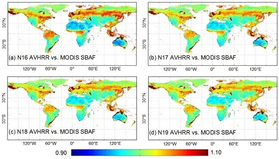
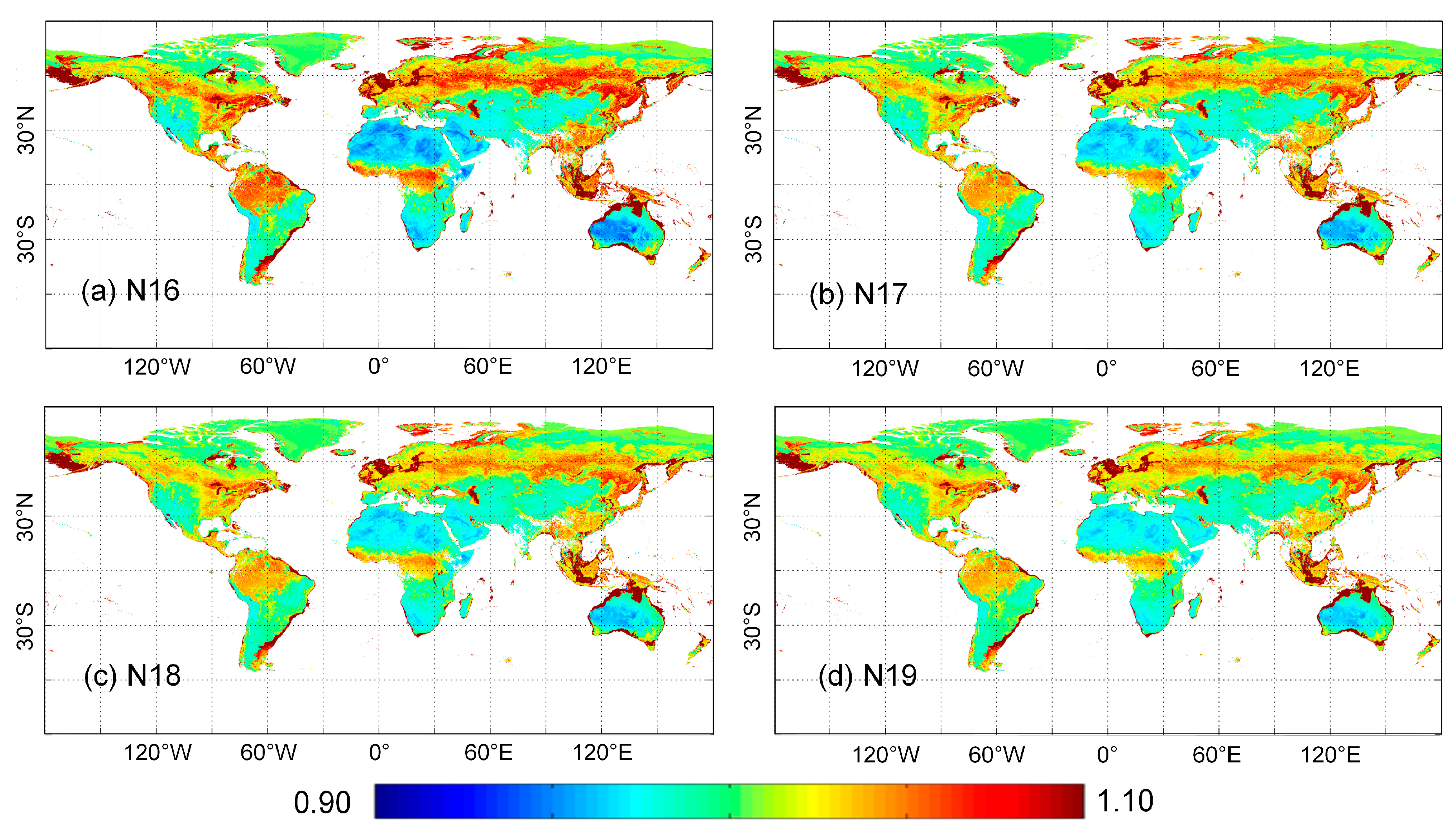
MODIS has provided accurate surface reflectance products, which enable global SBAF mapping. With the 16-day MODIS albedo data in DOY183, 2016, the global patterns of SBAF for NOAA-16~19 vs. MODIS are illustrated in Figure 7. The SBAFs show similar spatial patterns, and generally range between 0.90 and 1.10, indicative of <10% differences in MODIS and AVHRRs visible bands. High SBAF values are generally located around 60°N and near the equator, where dense vegetation is distributed. A majority of terrestrial surfaces has close-to-unity SBAF values, indicative of minor MODIS-AVHRR differences in the visible band. These surfaces are generally covered by sparse vegetation. The lowest SBAF values are observed in the North African deserts and the Australian barren lands. Note that the extremely large SBAF values are caused by offshore seawaters and inland waters. In summary, SBAFs are larger than unity for densely vegetated areas, and less than unity for dry bare lands. Soil moisture and vegetation cover increase SBAF values over the bare lands, leading to minor MODIS-AVHRRs differences. Sensor-to-sensor comparisons show that the contrast of global SBAF decreases gradually and more SBAF values are concentrated around unity from NOAA-16 to NOAA-19, indicating smaller differences between MODIS and modern AVHRRs.
Ongoing MODIS observations provide continuous MODIS surface reflectance data. With the 16-day MODIS albedo data in 2012–2016, the recent five years of SBAF values over stable desert sites are shown in Figure 8. Among the six desert sites, the Taklimakan site has the highest SBAF values (0.985–0.990), indicative of minor AVHRR-MODIS differences. SBAF values are similar for the Libya-4, Badain Jaran and Mali-1 sites (0.975–0.980). Low SBAF values occur at the Arabia-1 site (~0.970) and the Algeria-3 site (~0.965). No trends are detected in the time series SBAF data, indicating that all sites remain spectrally stable in the five years. However, the SBAFs show both seasonal and short-term variations. The former is probably associated with variations in solar angles, and the latter is probably associated with cloud contamination. Because the SBAFs are calculated using albedo data, the accuracy of BRDF modelling is critical. Frequent cloud coverage reduces angular sampling for BRDF modeling, and therefore may cause abrupt changes in the SBAF series. Relative to the Libya-4 site, the mid-latitude Taklimakan and Badain Jaran sites in China seem more affected by solar angles and cloud effects.
3.5. Results of SBAF Calculation for MODIS and AVHRR Observations
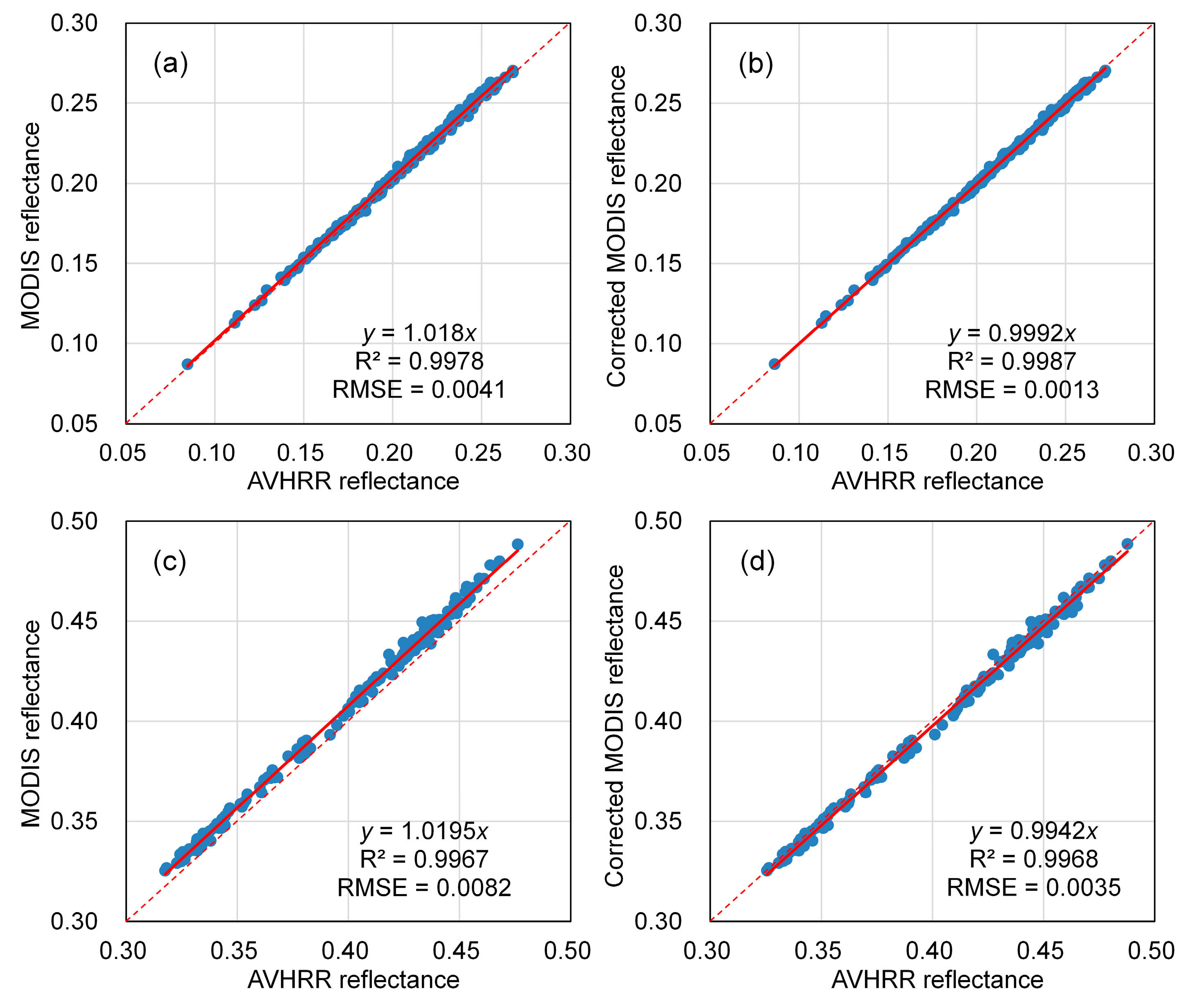
The above results are based on accurate references such as literature data, Hyperion reflectance or MODIS product. The performances of SBAF calculation in regard to real satellite observations are shown in Figure 9, respectively, for land surfaces near the low-to-moderate reflective Dunhuang site and the moderate-to-high reflective Libya-4 site. Before SBAF correction, the MODIS reflectances are approximately 1.80% and 1.95% higher than the AVHRR reflectances, respectively, for the two levels of reflective surfaces. After SBAF correction, however, the differences decrease substantially to −0.08% and −0.58% for the two surfaces. The reflectance pairs are more concentrated along the 1:1 line, also demonstrated by the increased R2 and decreased values after SBAF correction. Although the application to real satellite observations may be subject to many sources of uncertainty, the results are promising, at least for the two case studies. Overall, the method and derived SBAFs can improve MODIS-AVHRR data consistency in the visible band.
4. Discussion
4.1. Comparisons with the Hyperspectral Method
Spectral band differences are one of the critical issues to creating multisensor data consistency, and adjustment of these differences is required in particular for sensor intercalibration. Following the practice in sensor intercalibration, SBAF is used to quantify MODIS-AVHRRs reflectance differences in the visible band. The proposed SBAF calculation method in this study owns several advantages over existing methods, including better data availability, spatial resolution and temporal continuity. SBAFs are currently calculated using hyperspectral data, from either in situ measurements or satellite observations. The former can reflect site situation at specific time, while require much work especially for remote areas. In addition, SBAF varies with solar angles (Figure 8), and therefore multiple field campaigns are required to characterize annual SBAF variations, especially in mid-latitude and high-latitude regions. Satellite observations are acquired from Hyperion and SCIAMACHY. However, the narrow Hyperion swath width and the coarse SCIAMACHY spatial resolution may limit their use for sensor intercalibration. It is difficult to obtain SBAFs over sites that lack Hyperion coverage and are smaller than the SCIAMACHY footprint. To this end, the proposed method uses daily MODIS data, which provide more frequent coverage than Hyperion and finer spatial resolution than SCIAMACHY. At the MODIS spatial resolution, the proposed method fills scale gaps amid point scale measurement and ten-kilometer scale satellite observation. The other advantage is the temporal continuity of SBAF data as MODIS observations are still ongoing. SCIAMACHY has been decommissioned in 2012 and Hyperion in 2017. The derived SBAF data only serve as the priori knowledge, and are used under the assumption of unchanged land surfaces.
MODIS has several merits for SBAF calculation. First, the state-of-the-art sensor calibration and downstream data processing provide accurate surface reflectance data. Sensitivity analyses show that AOT and ozone concentration have a strong impact on SBAF calculation, especially over vegetated sites at high AOT levels (Figure 6). AOT is well retrievable from MODIS, and used for atmospheric correction. The retrievals are more reliable over vegetated areas. As a result, MODIS daily surface reflectance dataset has an overall uncertainty of 5%, which is favorable for SBAF calculation. Second, MODIS sensors are able to sample a variety of sun–target–sensor geometries. Most desert calibration sites are located in low-latitude areas where solar angles have a small dynamic range. The SBAFs are therefore stable across the whole year. In high-latitude areas, however, solar angles vary significantly. The SBAFs may have a wide dynamic range, which can be further complicated by varying sensor angles. In this sense, MODIS can provide SBAF data under various sun–target–sensor geometries. The angular dependence of SBAF can thus be investigated. The varying sun–target–sensor geometries coupled with topography may cause high variations in surface reflectances, especially for fine-resolution sensors such as Landsat Thematic Mapper (TM) [53,54]. However, topographic correction is generally less considered for coarse-resolution sensors such as MODIS and AVHRR. In practice, BRDF models are more effective to investigate the angular dependence of MODIS-AVHRR SBAFs.
4.2. Implications for Sensor Intercalibration
SBAF is initially proposed for sensor intercalibration. The derived 500-m SBAF data can improve MODIS-AVHRRs intercalibration in at least two aspects. First, the spatially detailed SBAFs provide an independent inspection of calibration site. The usable areas of most calibration sites are within the SCIAMACHY footprint (http://calvalportal.ceos.org/), and therefore the small-scale SBAF variations within a SCIAMACHY footprint cannot be captured. With the 500-m SBAF data, however, the spatial homogeneity can be evaluated. For instance, the Dunhuang site shows SBAF variations in the north-south direction (Figure 4c), which has been reported [55] and visually identified on satellite images. It is now possible to determine whether sensor intercalibration can meet accuracy requirements when taking the Dunhuang site as a whole calibration target. Second, time series SBAF data are available to evaluate the temporal stability of calibration sites and angular dependence of SBAF. The temporal stability can be fitted using time series data, e.g., no trends are detected for the desert sites in Figure 8. The archived and ongoing MODIS observations can be used in this fashion to evaluate current and potential calibration sites in regard to SBAF. The angular dependence of SBAF determines whether SBAF derived under different sun–target–sensor geometries can be used for sensor intercalibration. For instance, Wang et al. [38] state that nadir reflectances can be used for SBAF calculation when sensors share identical observational geometry. This can be further validated using the time series SBAF data in this study.
The method has significant implications for ray-matching based sensor intercalibration. The ray-matching technique provides more intercalibration opportunities, and has been widely used among many sensors [44]. The main idea is to screen for pair images (e.g., MODIS and AVHRR) that share similar sun–target–sensor geometries (indicative of similar sensor overpassing time), and compare dual-sensor observations for calibration bias. Determination of SBAFs is critical for such a technique, given that MODIS atmospheric products can account for the atmospheric differences [18]. For a matched site with mixed land cover types, the proposed method may provide ideal SBAF data in support of such intercalibration tasks. The MODIS data themselves are used instead of other ancillary data, which can reduce uncertainties related to spatial/angular mismatch and mixed pixels.
4.3. Implications for Spectral Band Conversions
The proposed method is actually a variant of spectral band conversion. Spectral band conversion normalizes multisensor data onto the same radiometric level that would be observed by a single sensor. For this purpose, linear regressions are mostly used, based on the fact of strong correlations between similar spectral bands. Linear regressions also apply to conversion of the derivative products, such as the Normalized Difference Vegetation Index (NDVI). Fan and Liu [26] demonstrate that the distributed (‘Band-to-NDVI’) scheme performs better than the lumped (‘NDVI-to-NDVI’) scheme. Therefore, the spectral band conversions can be improved for NDVI conversions. Aside from linear regression between analogous spectral bands, Gao and Kaufman [47] and Fan et al. [56] use two bands for conversion. This method is useful for analogous bands that show major SRF differences, such as narrow MODIS SRFs vs. wide AVHRRs SRFs. Multiple liner regressions are used in their studies for transformation equations, based on training samples. The transformed reflectance (e.g., AVHRR) is essentially the weighted average of reflectances at the two neighboring bands (e.g., MODIS). The proposed method in this study, however, exploits both nonlinear index and nonlinear transferring equations, which may add more information to spectral band conversions and therefore contribute to improved multisensor NDVI conversions.
Differences in spatial resolution should be considered for spectral band conversion. With respect to sensor intercalibration, SBAFs are calculated over homogeneous calibration sites. The differences in spatial resolution between e.g., MODIS and AVHRRs are less critical. However, this issue cannot be avoided for natural land surfaces, especially when the AVHRR Global Area Coverage (GAC) data are considered. In this study, the spatial scale mismatch between Hyperion and MODIS is processed by an aggregation method. Both data are aggregated into 1500 m × 1500 m grids (50 × 50 Hyperion pixels, or 3 × 3 MODIS pixels). Therefore, a coarser spatial resolution (lower than both MODIS and AVHRRs) should be used when applying the method for spectral band conversion.
5. Conclusions
This study proposes an SBAF calculation method for MODIS-AVHRRs in the visible band, in an initial effort to improve sensor intercalibration and a further implication for spectral band conversion. The method involves a uniform ratio index calculated using surface reflectance data at the MODIS 552-nm and 645-nm bands, and a sensor specific quadratic equation. The calculated SBAFs are in good agreement with the literature reported and Hyperion derived data, and significantly improve MODIS-AVHRR surface reflectance data consistency in the visible band. The relative SBAF error is <1.0% and the total uncertainty is ~0.001. Application of the SBAF data can reduce MODIS and AVHRR surface reflectance differences to within 1.0% reflectance units. Simulation results show strong SBAF sensitivities to aerosol scatting and ozone absorption, especially over the vegetated areas. At global scale, large SBAFs (>1.0) values are observed in densely vegetated areas, and low SBAFs (0.96–0.98) values are observed in the North African desert sites and the Australian barren lands. Desert sites generally exhibit stable SBAF values, although subject to BRDF effects. The MODIS based method provides continuing daily SBAF data under various sun–target–sensor geometries, and at spatial scales comparable to AVHRRs. It also fills the scale gaps between SBAF data from Hyperion and SCIAMACHY, which have already been decommissioned. The main idea behind this study would benefit ray-matching based sensor intercalibration and statistically based spectral band conversion. It is expected that the proposed method is transferrable to other types of sensors.
Acknowledgments
This study was jointly supported by the National Natural Science Foundation of China (41701414) and the Talent Introduction Project of the Nanjing Institute of Geography and Limnology, Chinese Academy of Sciences (NIGLAS2015QD08). The authors would like to thank the anonymous reviewers for their constructive comments on an early version of this paper. The MODIS data were collected from the Level-1 and Atmosphere Archive & Distribution System (LAADS) Distributed Active Archive Center (DAAC), Goddard Space Flight Center, and the AVHRR data from the Comprehensive Large Array-data Stewardship System (CLASS), NOAA, and the Hyperion data from the Earth Resources Observation and Science Center (EROS), USGS, and the MODIS SRF data from the OceanColor website, and the AVHRR SRF data from the National Centers for Environmental Information (NCEI), NOAA.
Author Contributions
Xingwang Fan and Yuanbo Liu conceived and designed the experiments; Xingwang Fan analyzed the data and wrote the paper.
Conflicts of Interest
The authors declare no conflict of interest.
References
- Lautenbacher, C.C. The global earth observation system of systems: Science serving society. Space Policy 2006, 22, 8–11. [Google Scholar] [CrossRef]
- Belward, A.S.; Skøien, J.O. Who launched what, when and why; trends in global land-cover observation capacity from civilian earth observation satellites. ISPRS J. Photogramm. 2015, 103, 115–128. [Google Scholar] [CrossRef]
- Pinzon, J.E.; Tucker, C.J. A non-stationary 1981–2012 AVHRR NDVI3g time series. Remote Sens. 2014, 6, 6929–6960. [Google Scholar] [CrossRef]
- Roy, D.P.; Kovalskyy, V.; Zhang, H.K.; Vermote, E.F.; Yan, L.; Kumar, S.S.; Egorov, A. Characterization of Landsat-7 to Landsat-8 reflective wavelength and normalized difference vegetation index continuity. Remote Sens. Environ. 2016, 185, 57–70. [Google Scholar] [CrossRef]
- Gao, F.; Masek, J.; Schwaller, M.; Hall, F. On the blending of the Landsat and MODIS surface reflectance: Predicting daily Landsat surface reflectance. IEEE Trans. Geosci. Remote Sens. 2006, 44, 2207–2218. [Google Scholar]
- Van der Werff, H.; van der Meer, F. Sentinel-2A MSI and Landsat 8 OLI provide data continuity for geological remote sensing. Remote Sens. 2016, 8, 883. [Google Scholar] [CrossRef]
- Kennedy, R.E.; Andréfouët, S.; Cohen, W.B.; Gómez, C.; Griffiths, P.; Hais, M.; Healey, S.P.; Helmer, E.H.; Hostert, P.; Lyons, M.B.; et al. Bringing an ecological view of change to Landsat-based remote sensing. Front. Ecol. Environ. 2014, 12, 339–346. [Google Scholar] [CrossRef] [Green Version]
- Khlopenkov, K.V.; Trishchenko, A.P. SPARC: New cloud, snow, and cloud shadow detection scheme for historical 1-km AVHHR data over Canada. J. Atmos. Ocean. Technol. 2007, 24, 322–343. [Google Scholar] [CrossRef]
- Xue, Y.; He, X.; de Leeuw, G.; Mei, L.; Che, Y.; Rippin, W.; Guang, J.; Hu, Y. Long-time series aerosol optical depth retrieval from AVHRR data over land in North China and Central Europe. Remote Sens. Environ. 2017, 198, 471–489. [Google Scholar] [CrossRef]
- Bhatt, R.; Doelling, D.R.; Scarino, B.R.; Gopalan, A.; Haney, C.O.; Minnis, P.; Bedka, K.M. A consistent AVHRR visible calibration record based on multiple methods applicable for the NOAA degrading orbits. Part I: Methodology. J. Atmos. Ocean. Technol. 2016, 33, 2499–2515. [Google Scholar] [CrossRef]
- Chander, G.; Hewison, T.J.; Fox, N.; Wu, X.; Xiong, X.; Blackwell, W.J. Overview of intercalibration of satellite instruments. IEEE Trans. Geosci. Remote Sens. 2013, 51, 1056–1080. [Google Scholar] [CrossRef]
- Xiong, X.; Barnes, W. An overview of MODIS radiometric calibration and characterization. Adv. Atmos. Sci. 2006, 23, 69–79. [Google Scholar] [CrossRef]
- Vermote, E.F.; Saleous, N.Z. Calibration of NOAA16 AVHRR over a desert site using MODIS data. Remote Sens. Environ. 2006, 105, 214–220. [Google Scholar] [CrossRef]
- Zhong, B.; Yang, A.; Wu, S.; Li, J.; Liu, S.; Liu, Q. Cross-calibration of reflective bands of major moderate resolution remotely sensed data. Remote Sens. Environ. 2018, 204, 412–423. [Google Scholar] [CrossRef]
- Chander, G.; Xiong, X.J.; Choi, T.J.; Angal, A. Monitoring on-orbit calibration stability of the Terra MODIS and Landsat 7 ETM+ sensors using pseudo-invariant test sites. Remote Sens. Environ. 2010, 114, 925–939. [Google Scholar] [CrossRef]
- Gitelson, A.A.; Kaufman, Y.J. MODIS NDVI optimization to fit the AVHRR data series—Spectral considerations. Remote Sens. Environ. 1998, 66, 343–350. [Google Scholar] [CrossRef]
- Trishchenko, A.P.; Cihlar, J.; Li, Z. Effects of spectral response function on surface reflectance and NDVI measured with moderate resolution satellite sensors. Remote Sens. Environ. 2002, 81, 1–18. [Google Scholar] [CrossRef]
- Fan, X.; Liu, Y. Intercalibrating the MODIS and AVHRR visible bands over homogeneous land surfaces. IEEE Geosci. Remote Sens. Lett. 2018, 15, 83–87. [Google Scholar] [CrossRef]
- Desormeaux, Y.; Rossow, W.B.; Brest, C.L.; Campbell, G.G. Normalization and calibration of geostationary satellite radiances for the International Satellite Cloud Climatology Project. J. Atmos. Ocean. Technol. 1993, 10, 304–325. [Google Scholar] [CrossRef]
- Minnis, P.; Nguyen, L.; Doelling, D.R.; Young, D.F.; Miller, W.F.; Kratz, D.P. Rapid calibration of operational and research meteorological satellite imagers. Part I: Evaluation of research satellite visible channels as references. J. Atmos. Ocean. Technol. 2002, 19, 1233–1249. [Google Scholar] [CrossRef]
- Galvão, L.S.; Vitorello, Í.; Almeida Filho, R. Effects of band positioning and bandwidth on NDVI measurements of tropical savannas. Remote Sens. Environ. 1999, 67, 181–193. [Google Scholar] [CrossRef]
- Teillet, P.M.; Barker, J.L.; Markham, B.L.; Irish, R.R.; Fedosejevs, G.; Storey, J.C. Radiometric cross-calibration of the Landsat-7 ETM+ and Landsat-5 TM sensors based on tandem data sets. Remote Sens. Environ. 2001, 78, 39–54. [Google Scholar] [CrossRef]
- Cao, C.; Xiong, X.; Wu, A.; Wu, X. Assessing the consistency of AVHRR and MODIS L1B reflectance for generating fundamental climate data records. J. Geophys. Res. Atmos. 2008, 113. [Google Scholar] [CrossRef]
- Sayer, A.M.; Thomas, G.E.; Grainger, R.G.; Carboni, E.; Poulsen, C.; Siddans, R. Use of MODIS-derived surface reflectance data in the ORAC-AATSR aerosol retrieval algorithm: Impact of differences between sensor spectral response functions. Remote Sens. Environ. 2012, 116, 177–188. [Google Scholar] [CrossRef]
- Fan, X.; Liu, Y. A Generalized model for intersensor NDVI calibration and its comparison with regression approaches. IEEE Trans. Geosci. Remote Sens. 2017, 55, 1842–1852. [Google Scholar] [CrossRef]
- Fan, X.; Liu, Y. A comparison of NDVI intercalibration methods. Int. J. Remote Sens. 2017, 38, 5273–5290. [Google Scholar] [CrossRef]
- Steven, M.D.; Malthus, T.J.; Baret, F.; Xu, H.; Chopping, M.J. Intercalibration of vegetation indices from different sensor systems. Remote Sens. Environ. 2003, 88, 412–422. [Google Scholar] [CrossRef]
- D’Odorico, P.; Gonsamo, A.; Damm, A.; Schaepman, M.E. Experimental evaluation of Sentinel-2 spectral response functions for NDVI time-series continuity. IEEE Trans. Geosci. Remote Sens. 2013, 51, 1336–1348. [Google Scholar] [CrossRef]
- Thenkabail, P.S. Inter-sensor relationships between IKONOS and Landsat-7 ETM+ NDVI data in three ecoregions of Africa. Int. J. Remote Sens. 2004, 25, 389–408. [Google Scholar] [CrossRef]
- Miura, T.; Huete, A.; Yoshioka, H. An empirical investigation of cross-sensor relationships of NDVI and red/near-infrared reflectance using EO-1 Hyperion data. Remote Sens. Environ. 2006, 100, 223–236. [Google Scholar] [CrossRef]
- Gonsamo, A.; Chen, J.M. Spectral response function comparability among 21 satellite sensors for vegetation monitoring. IEEE Trans. Geosci. Remote Sens. 2013, 51, 1319–1335. [Google Scholar] [CrossRef]
- Chander, G.; Mishra, N.; Helder, D.L.; Aaron, D.B.; Angal, A.; Choi, T.; Xiong, X.; Doelling, D.R. Applications of spectral band adjustment factors (SBAF) for cross-calibration. IEEE Trans. Geosci. Remote Sens. 2013, 51, 1267–1281. [Google Scholar] [CrossRef]
- Chander, G.; Angal, A.; Choi, T.; Meyer, D.J.; Xiong, X.; Teillet, P.M. Cross-calibration of the Terra MODIS, Landsat 7 ETM+ and EO-1 ALI sensors using near-simultaneous surface observation over the Railroad Valley Playa, Nevada, test site. In Proceedings of the SPIE 6677, Earth Observing Systems XII, San Diego, CA, USA, 26–28 August 2007. [Google Scholar]
- Choi, T.; Xiong, X.; Angal, A.; Chander, G. Simulation of the long term radiometric responses of the Terra MODIS and EO-1 ALI using Hyperion spectral responses over Railroad Valley Playa in Nevada (RVPN). In Proceedings of the SPIE 7862, Earth Observing Missions and Sensors: Development, Implementation, and Characterization, Incheon, Korea, 11–14 October 2010. [Google Scholar]
- Li, X.; Gu, X.; Min, X.; Yu, T.; Fu, Q.; Zhang, Y.; Li, X. Radiometric cross-calibration of the CBERS-02 CCD camera with the TERRA MODIS. Sci. China Ser. E 2005, 48, 44–60. [Google Scholar]
- Teillet, P.M.; Fedosejevs, G.; Thome, K.J.; Barker, J.L. Impacts of spectral band difference effects on radiometric cross-calibration between satellite sensors in the solar-reflective spectral domain. Remote Sens. Environ. 2007, 110, 393–409. [Google Scholar] [CrossRef]
- Wu, A.; Xiong, X.; Jin, Z.; Lukashin, C.; Wenny, B.N.; Butler, J.J. Sensitivity of intercalibration uncertainty of the CLARREO reflected solar spectrometer features. IEEE Trans. Geosci. Remote Sens. 2015, 53, 4741–4751. [Google Scholar] [CrossRef]
- Wang, Z.; Xiao, P.; Gu, X.; Feng, X.; Li, X.; Gao, H.; Li, H.; Lin, J.; Zhang, X. Uncertainty analysis of cross-calibration for HJ-1 CCD camera. Sci. China Ser. E 2013, 56, 713–723. [Google Scholar] [CrossRef]
- Teillet, P.M.; Slater, P.N.; Ding, Y.; Santer, R.P.; Jackson, R.D.; Moran, M.S. Three methods for the absolute calibration of the NOAA AVHRR sensors in-flight. Remote Sens. Environ. 1990, 31, 105–120. [Google Scholar] [CrossRef]
- Röder, A.; Kuemmerle, T.; Hill, J. Extension of retrospective datasets using multiple sensors. An approach to radiometric intercalibration of Landsat TM and MSS data. Remote Sens. Environ. 2005, 95, 195–210. [Google Scholar] [CrossRef]
- Henry, P.; Chander, G.; Fougnie, B.; Thomas, C.; Xiong, X. Assessment of spectral band impact on intercalibration over desert sites using simulation based on EO-1 Hyperion data. IEEE Trans. Geosci. Remote Sens. 2013, 51, 1297–1308. [Google Scholar] [CrossRef]
- Feng, L.; Li, J.; Gong, W.; Zhao, X.; Chen, X.; Pang, X. Radiometric cross-calibration of Gaofen-1 WFV cameras using Landsat-8 OLI images: A solution for large view angle associated problems. Remote Sens. Environ. 2016, 174, 56–68. [Google Scholar] [CrossRef]
- Li, J.; Feng, L.; Pang, X.; Gong, W.; Zhao, X. Radiometric cross Calibration of Gaofen-1 WFV Cameras Using Landsat-8 OLI Images: A Simple Image-Based Method. Remote Sens. 2016, 8, 411. [Google Scholar] [CrossRef]
- Doelling, D.R.; Scarino, B.R.; Morstad, D.; Gopalan, A.; Bhatt, R.; Lukashin, C.; Minnis, P. The intercalibration of geostationary visible imagers using operational hyperspectral SCIAMACHY radiances. IEEE Trans. Geosci. Remote Sens. 2013, 51, 1245–1254. [Google Scholar] [CrossRef]
- Scarino, B.R.; Doelling, D.R.; Minnis, P.; Gopalan, A.; Chee, T.; Bhatt, R.; Lukashin, C.; Haney, C. A web-based tool for calculating spectral band difference adjustment factors derived from SCIAMACHY hyperspectral data. IEEE Trans. Geosci. Remote Sens. 2016, 54, 2529–2542. [Google Scholar] [CrossRef]
- Clark, R.N.; Swayze, G.A.; Wise, R.; Livo, K.E.; Hoefen, T.; Kokaly, R.F.; Sutley, S.J. USGS Digital Spectral Library Splib06a; Digital Data Series 231; United States Geological Survey: Reston, VA, USA, 2007.
- Gao, B.C.; Kaufman, Y.J. Water vapor retrievals using Moderate Resolution Imaging Spectroradiometer (MODIS) near-infrared channels. J. Geophys. Res. Atmos. 2003, 108, 4389. [Google Scholar] [CrossRef]
- Fan, X.; Liu, Y. Quantifying the relationship between intersensor images in solar reflective bands: Implications for intercalibration. IEEE Trans. Geosci. Remote Sens. 2014, 52, 7727–7737. [Google Scholar]
- Weng, Y.; Gong, P.; Zhu, Z. Reflectance spectroscopy for the assessment of soil salt content in soils of the Yellow River Delta of China. Int. J. Remote Sens. 2008, 29, 5511–5531. [Google Scholar] [CrossRef]
- Vermote, E.F.; Tanré, D.; Deuze, J.L.; Herman, M.; Morcette, J.J. Second simulation of the satellite signal in the solar spectrum, 6S: An overview. IEEE Trans. Geosci. Remote Sens. 1997, 35, 675–686. [Google Scholar] [CrossRef]
- Vermote, E.F.; Vermeulen, A. Atmospheric Correction Algorithm: Spectral Reflectances (MOD09); ATBD Version, 4; Department of Geography, University of Maryland: College Park, MD, USA, 1999. [Google Scholar]
- Heidinger, A.K.; Cao, C.; Sullivan, J.T. Using Moderate Resolution Imaging Spectrometer (MODIS) to calibrate advanced very high resolution radiometer reflectance channels. J. Geophys. Res. Atmos. 2002, 107, AAC11-1–AAC11-10. [Google Scholar] [CrossRef]
- Riaño, D.; Chuvieco, E.; Salas, J.; Aguado, I. Assessment of different topographic corrections in Landsat-TM data for mapping vegetation types. IEEE Trans. Geosci. Remote Sens. 2003, 41, 1056–1061. [Google Scholar] [CrossRef]
- Pons, X.; Pesquer, L.; Cristóbal, J.; González-Guerrero, O. Automatic and improved radiometric correction of Landsat imagery using reference values from MODIS surface reflectance images. Int. J. Appl. Earth Obs. 2014, 33, 243–254. [Google Scholar] [CrossRef]
- Liu, J.J.; Li, Z.; Qiao, Y.L.; Liu, Y.J.; Zhang, Y.X. A new method for cross-calibration of two satellite sensors. Int. J. Remote Sens. 2004, 25, 5267–5281. [Google Scholar] [CrossRef]
- Fan, X.; Weng, Y.; Tao, J. Towards decadal soil salinity mapping using Landsat time series data. Int. J. Appl. Earth Obs. 2006, 52, 32–41. [Google Scholar] [CrossRef]
Figure 1.
Spectral response functions of (a) AVHRR/1-2; (b) AVHRR/3 and MODIS/Terra in the visible band.
Figure 1.
Spectral response functions of (a) AVHRR/1-2; (b) AVHRR/3 and MODIS/Terra in the visible band.
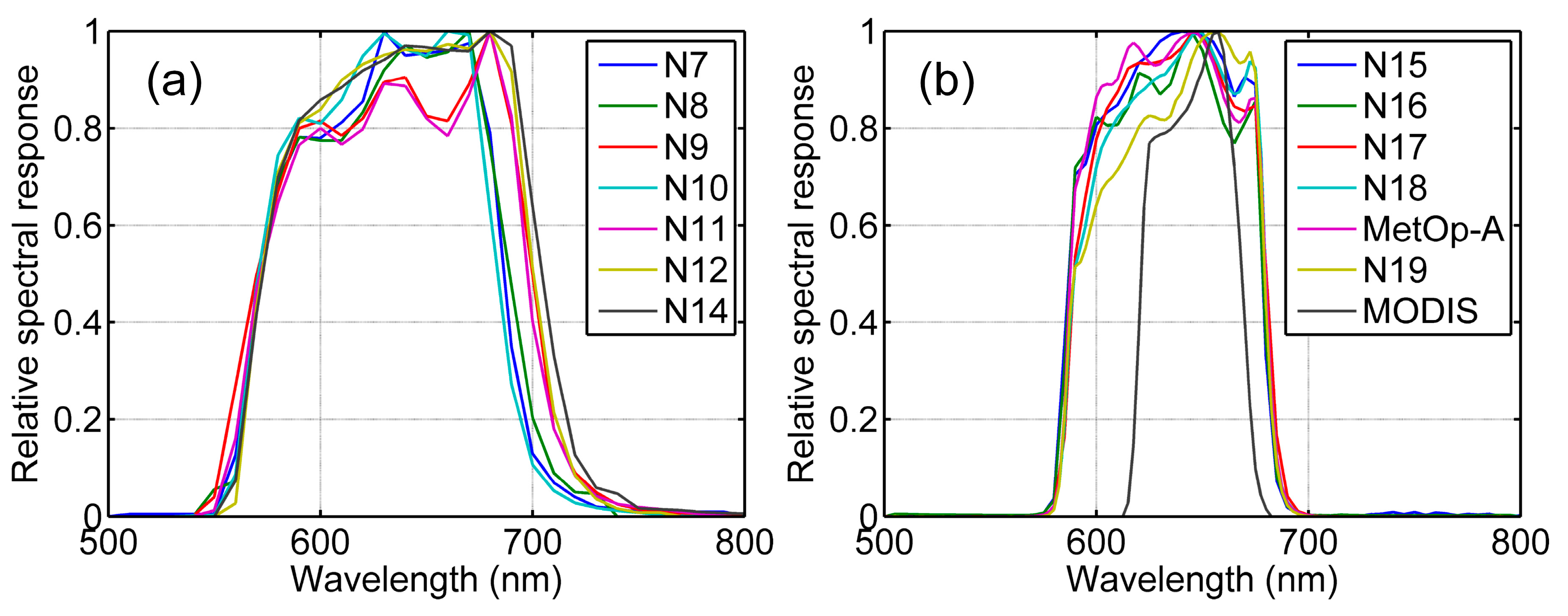
Figure 2.
(a) Terra MODIS and (b) NOAA-17 AVHRR visible band observations near the Dunhuang site (DOY116, 2004), and (c) Terra MODIS and (d) NOAA-17 AVHRR visible band observations near the Libya-4 site (DOY113, 2004). The MODIS and AVHRRL1B observations are shown as MODIS Scaled Integer (SI) and AVHRR Digital Count (DC).
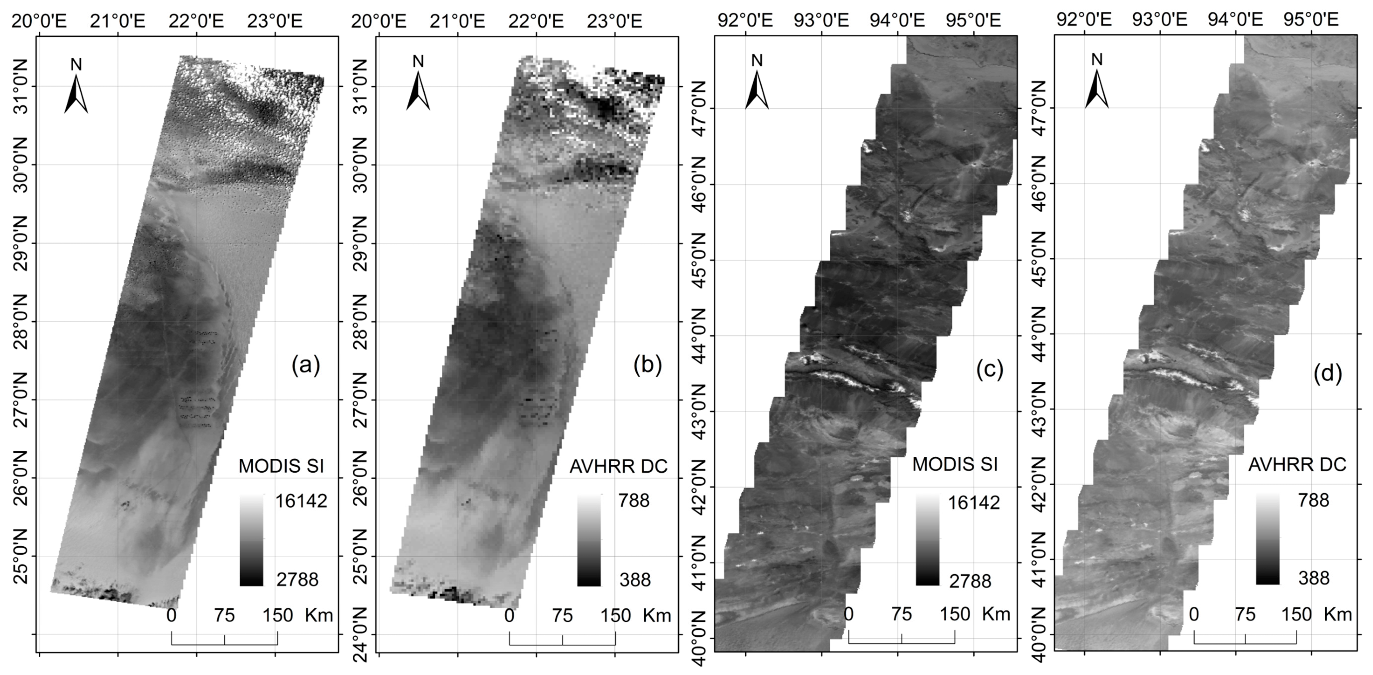
Figure 3.
The flowchart of SBAF calculation, validation and application.

Figure 4.
The MODIS based SBAFs for (a) NOAA-16 over the Libya-4 site on 30 April 2015, (b) NOAA-16 over the Libya-4 site on 16 May 2015, (c) NOAA-17 over the Dunhuang site on 7 November 2002, (d) NOAA-16 over the Badain Jaran site on 13 July 2012, (e) NOAA-17 over the Badain Jaran site on 13 July 2012, and (f) NOAA-18 over the Badain Jaran site on 13 July 2012.

Figure 5.
Top: Comparisons of the Hyperion-derived and MODIS calculated SBAFs in the case of NOAA-19 AVHRR vs. MODIS around (a) the Libya-4 site on 30 April 2005, (b) the Libya-4 site on 16 May 2015, and (c) the Yellow River Delta on 14 April 2005. Bottom: Remotely sensed data of the Yellow River Delta, including (c-1) the Hyperion false color composite map (R = 854 nm, G = 651 nm, B = 549 nm), (c-2) the Hyperion simulated MODIS reflectance, (c-3) the MODIS retrieved surface reflectance, and (c-4) the MODIS calculated SBAF. All data are resized according to the Hyperion spatial coverage.
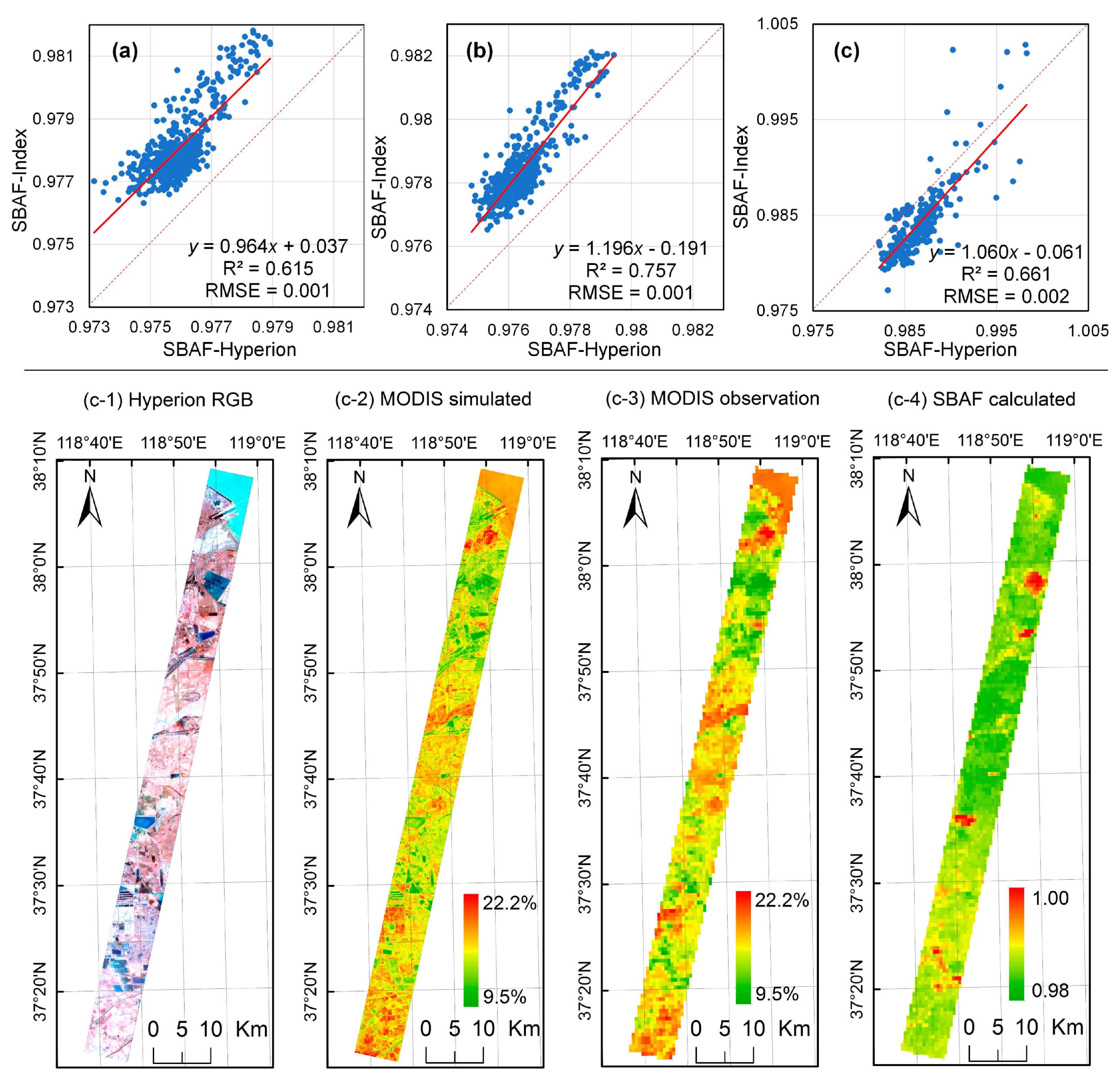
Figure 6.
SBAF sensitivities to AOT and ozone concentration in the case of NOAA-19 AVHRR vs. MODIS over (a) nonvegetated and (b) vegetated sites. The color map shows relative difference against SBAF calculated using surface reflectances.
Figure 6.
SBAF sensitivities to AOT and ozone concentration in the case of NOAA-19 AVHRR vs. MODIS over (a) nonvegetated and (b) vegetated sites. The color map shows relative difference against SBAF calculated using surface reflectances.

Figure 7.
Global patterns of SBAF for (a) NOAA-16 AVHRR, (b) NOAA-17 AVHRR, (c) NOAA-18 AVHRR, and (d) BOAA-19 AVHRR in middle 2016 (DOY = 183).
Figure 7.
Global patterns of SBAF for (a) NOAA-16 AVHRR, (b) NOAA-17 AVHRR, (c) NOAA-18 AVHRR, and (d) BOAA-19 AVHRR in middle 2016 (DOY = 183).

Figure 8.
Five years (2012–2016) of NOAA-19 AVHRR vs. MODIS SBAFs at the Taklimakan (39.83°N, 80.17°E), Libya (29.0°N, 23.8°E), Badain Jaran (39.9°N, 101.9°E), Mali (19.12°N, 4.85°W), Arabia (18.88°N, 46.76°E) and Algeria (30.32°N, 7.66°E) desert sites.
Figure 8.
Five years (2012–2016) of NOAA-19 AVHRR vs. MODIS SBAFs at the Taklimakan (39.83°N, 80.17°E), Libya (29.0°N, 23.8°E), Badain Jaran (39.9°N, 101.9°E), Mali (19.12°N, 4.85°W), Arabia (18.88°N, 46.76°E) and Algeria (30.32°N, 7.66°E) desert sites.
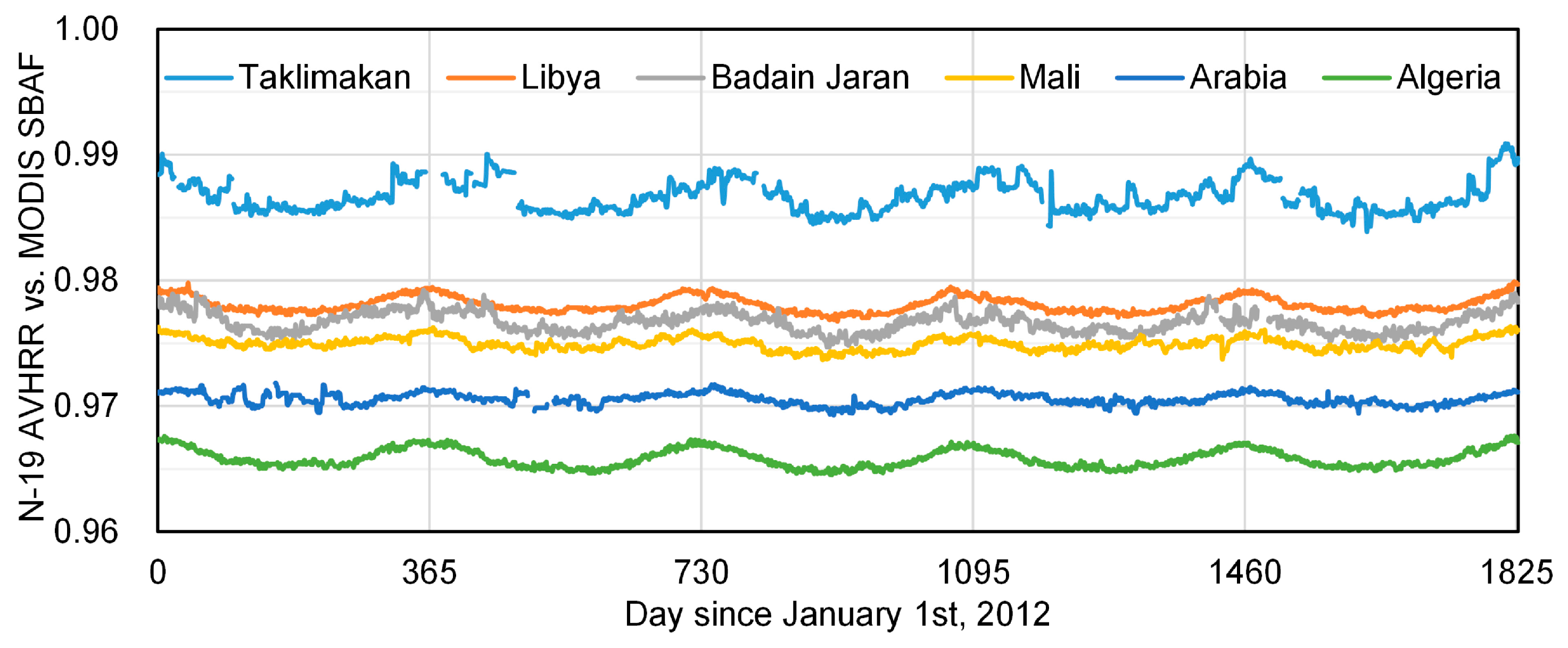
Figure 9.
Comparison of MODIS and AVHRR visible band surface reflectances before and after SBAF correction near the Dunhuang site (a,b), and the Libya-4 site (c,d).
Figure 9.
Comparison of MODIS and AVHRR visible band surface reflectances before and after SBAF correction near the Dunhuang site (a,b), and the Libya-4 site (c,d).

Table 1.
Sensor specific equations of SBAF and the MODIS index.
| Sensor | Equation (y = a2 × MOD_Ind2 + a1 × MOD_Ind + a0) | R2 | RMSE | ||
|---|---|---|---|---|---|
| Quadratic Term (a2) | Linear Term (a1) | Constant (a0) | |||
| N7 | 0.472 | −0.671 | 1.003 | 0.793 | 0.019 |
| N8 | 0.496 | −0.633 | 1.003 | 0.779 | 0.019 |
| N9 | 0.828 | −0.600 | 1.005 | 0.622 | 0.027 |
| N10 | 0.333 | −0.725 | 1.002 | 0.840 | 0.017 |
| N11 | 0.787 | −0.549 | 1.005 | 0.562 | 0.028 |
| N12 | 0.880 | −0.471 | 1.006 | 0.418 | 0.034 |
| N14 | 0.841 | −0.419 | 1.006 | 0.381 | 0.033 |
| N15 | −0.047 | −0.448 | 1.001 | 0.747 | 0.014 |
| N16 | −0.049 | −0.480 | 1.001 | 0.769 | 0.014 |
| N17 | −0.064 | −0.392 | 1.000 | 0.736 | 0.012 |
| N18 | −0.045 | −0.368 | 1.001 | 0.738 | 0.011 |
| MetOp−A | −0.098 | −0.439 | 1.000 | 0.743 | 0.013 |
| N19 | −0.007 | −0.349 | 1.001 | 0.755 | 0.010 |
Table 2.
Relative SBAF errors over sensor calibration sites.
| Site | Sensor | Literature Data | Calculated | Relative Difference |
|---|---|---|---|---|
| Niger desert | N16 | 0.952 | 0.964 | +1.2% |
| Dunhuang | N17 | 0.993 | 0.987 | −0.6% |
| Badain Jaran | N16 | 0.976 | 0.969 | −0.7% |
| Badain Jaran | N17 | 0.980 | 0.974 | −0.6% |
| Badain Jaran | N18 | 0.982 | 0.977 | −0.5% |
© 2018 by the authors. Licensee MDPI, Basel, Switzerland. This article is an open access article distributed under the terms and conditions of the Creative Commons Attribution (CC BY) license (http://creativecommons.org/licenses/by/4.0/).
Share and Cite
MDPI and ACS Style
Fan, X.; Liu, Y. Using a MODIS Index to Quantify MODIS-AVHRRs Spectral Differences in the Visible Band. Remote Sens. 2018, 10, 61. https://doi.org/10.3390/rs10010061
AMA Style
Fan X, Liu Y. Using a MODIS Index to Quantify MODIS-AVHRRs Spectral Differences in the Visible Band. Remote Sensing. 2018; 10(1):61. https://doi.org/10.3390/rs10010061
Chicago/Turabian StyleFan, Xingwang, and Yuanbo Liu. 2018. "Using a MODIS Index to Quantify MODIS-AVHRRs Spectral Differences in the Visible Band" Remote Sensing 10, no. 1: 61. https://doi.org/10.3390/rs10010061
Note that from the first issue of 2016, this journal uses article numbers instead of page numbers. See further details here.