Abstract
Dust devils are low-pressure, small (many to tens of meters) convective vortices powered by surface heating and rendered visible by lofted dust. Dust devils occur ubiquitously on Mars, where they may dominate the supply of atmospheric dust, and since dust contributes significantly to Mars’ atmospheric heat budget, dust devils probably play an important role in its climate. The dust-lifting capacity of a devil likely depends sensitively on its structure, particularly the wind and pressure profiles, but the exact dependencies are poorly constrained. Thus, the exact contribution to Mars’ atmosphere remains unresolved. Analog studies of terrestrial devils have provided some insights into dust devil dynamics and properties but have been limited to near-surface (few meters) or relatively high altitude (hundreds of meters) sampling. Automated aerial vehicles or drones, combined with miniature, digital instrumentation, promise a novel and uniquely powerful platform from which to sample dust devils at a wide variety of altitudes. In this article, we describe a pilot study using an instrumented quadcopter on an active field site in southeastern Oregon, which (to our knowledge) has not previously been surveyed for dust devils. We present preliminary results from the encounters, including stereo image analysis and encounter footage collected onboard the drone. In spite of some technical difficulties, we show that a quadcopter can successfully navigate in an active dust devil, while collecting time-series data about the dust devil’s structure.
1. Introduction
Powered by surface heating, dust devils are low-pressure convective vortices rendered visible by lofted dust. On Earth, they occur primarily in arid regions, have diameters of a few to tens of meters, can significantly degrade air quality [1], and may pose an aviation hazard [2]. Widespread across Mars, dust devils may grow as large as a kilometer, pose a hazard for human exploration [3], and may have lengthened the operational lifetime of rovers [4].
On Mars, dust devils probably also play a key role in maintaining the level of background dust in the atmosphere. Although global and regional dust storms lift significant dust, easily obscuring the surface [5], they occur every three years on average, e.g., [6]. With a settling timescale of perhaps only weeks [5], the global dust must be resupplied more frequently. Given their frequency and ubiquity, dust devils seem to be responsible. Martian dust absorbs and re-emits short-wave radiation, warming the atmosphere by tens of degrees K [7,8]. Thus, dust-lifting by devils on Mars is critical to the Martian climate.
However, the relationship between a dust devil’s physical properties, the tangential windspeed at its eyewall and the low-pressure excursion at its center , and its dust-lifting capacity are unclear. Based on analog experiments designed to mimic Martian dust devils, Neakrase and Greeley [9] suggested that the dust flux generated increases as roughly . Whether these lab experiments can be directly translated to dust devils in the field is unclear, though. Similar to the work described here, terrestrial field studies, cf. [10], have served as an important check on dust devil dynamical and structural relationships developed in the lab and in theory.
Indeed, theoretical work provides some guidance regarding the relationship between a dust devil’s various physical parameters. The seminal analysis in Rennó et al. [11] treats the dust devil as a thermodynamic heat engine, with heat input at the surface, buoyed up the dust devil column and then radiated out the top of the planetary boundary layer (PBL). This model predicts that is exponentially dependent on the temperature excursion powered by surface heating. Moreover, the thermodynamic efficiency of the devil depends on the difference between the central temperature and temperature at the top of the PBL. Dimensional analyses also suggest that dust devil height should scale with depth of the PBL [12]. However, this model does not predict the lateral structure of the dust devil, i.e., the pressure and wind profiles as a function of radial distance r. Instead, dynamical considerations must be invoked, and several vortex profiles have been proposed [13], including the Lorentz profile:
where is the pressure excursion measured at radial distance r, is the dust devil’s full-width at half maximum, and V is the tangential windspeed at r. is also often taken as the diameter of the dust devil eye wall. To date, only a few direct comparisons between theory and measurements of dust devils have been made. Using data from the Mars Pathfinder meteorology package, for example, Rennó et al. [14] found good agreement between predicted and observed dust devil pressures and wind speeds but only for the handful of dust devil encounters recovered. Similar experiments involving in situ deployment of time-series sensors on the Earth have also been conducted [15].
One drawback of these passive surveys is that encounter geometries between the dust devil and instrument pack are random, introducing non-trivial biases into the recovered population [16]. For example, the largest, most long-lived devils will be over-represented, but recent modeling efforts have begun to provide methods to ameliorate these biases [17]. Perhaps a more important bias for these surveys is that dust devils are unlikely to pass directly over the sensor package, i.e., the miss distance is non-zero, which means that the pressure, temperature, and wind profiles recovered do not directly reflect the values at the dust devil center. Instead, they represent a convolution between the intrinsic properties of the devil and the encounter geometry. Other studies have actively chased dust devils in order to probe their structures using instruments mounted on vehicles [18,19], allowing a more controlled encounter geometry, but both kinds of studies, active and passive, have usually been limited to measuring near-surface properties of dust devils (although seminal work in [20] used a sailplane to sample dust devil thermals at altitudes above 2000 ft.).
To address these shortcomings, we conducted a pilot study using an instrumented quadcopter or drone on the Alvord Desert playa in southeastern Oregon, a site that, to our knowledge, has never before been surveyed for dust devils. Such a sampling platform, in principle, allows us to control (or at least, monitor) the encounter geometry and to probe altitudes otherwise inaccessible to other platforms. As discussed below, our drone survived about half a dozen encounters with dust devils and successfully collected pressure and altitude time-series from on-board the drone during these encounters. We conducted a detailed time-series analysis to recover the pressure signals resulting from these dust devils. In order to monitor the encounter geometries, we also attempted to collect simultaneous stereo-imaging. Although the limited success of our stereo-imaging hindered a robust assessment of the dust devils’ pressure profiles, the primary goal of our survey was simply to show that the drone could stably navigate and pass through a dust devil. With this success from the pilot study, we have shown that probing dust devils with this unique platform has tremendous potential to reveal novel insights into dust devil dynamics and processes.
2. Materials and Methods
For our pilot study, we visited the Alvord Desert (Figure 1), a roughly 7 × 12 km dry lake bed in southeastern Oregon. The Alvord Desert is located in Harney County, Oregon and lies near the northernmost end of the Basin and Range province of the southwestern United States. The basin is a broad, flat, graben valley bounded by Steens Mountain to the northwest and hosts several hot springs, including the Alvord Hot Springs adjacent to the playa. As a local catchment for infrequent rain and snowmelt, the Alvord playa is layered with brightly colored, fine silt, ideally suited for visualizing active convective cells and producing dust devils. Indeed, reports from the owners of the Alvord Desert Hot Springs, located adjacent to the playa, suggested frequent dust devil activity. We confirmed this report by conducting a short time-lapse survey during which we deployed cameras to monitor the playa over the course of a few weeks.
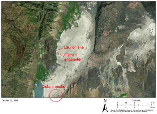
Figure 1.
Landsat image of Alvord Desert, courtesy of NASA Goddard Space Flight Center and the U.S. Geological Survey. The figure shows the approximate launch site, adjacent to the playa access road, and the location of the Flight 1 dust devil encounter. The distant peaks against which we estimated parallax are also shown.
For our drone survey, we visited Alvord on 20 and 21 July. An initial attempt on 20 July to actively pursue dust devils from our vehicle before deploying the drone was unsuccessful, so instead on, 21 July, we established a fixed launch site near the access road to the playa on its western margin. From this location, we launched the instrumented drone and videoed or photographed the dust devil encounters. In the following, we describe our equipment and detail our field set-up. Worth noting, the cameras we used had dust protection, but none of the other equipment had significant protection, which did not seem to affect their operation
2.1. Stereo Cameras
We used simple point-and-click cameras, Ricoh WG-5 GPS (Chuo, Tokyo, Japan), to image the encounters. The Ricoh WG-5 GPS has default resolutions of 4608 × 2592 pixels in still mode and 1920 × 1080 in video mode (which records at 30 frames-per-second). In both modes, the field of view is 71.5 × 40.2 when not zoomed in, which we did not do. We used the default “Auto Picture” setting, which automatically adjusts the camera settings since our study did not require photometrically or chromatically controlled images. With onboard barometers, digital compasses, digital level meters, and pressure sensors, the cameras also record GPS location, bearing, and altitude information directly into the image meta-data, although the uncertainties in these data are not provided. Of particular relevance to our study, the cameras have a Japanese Industrial Standard Dust Ingress Protection grade of six, meaning they are dust tight and should allow no ingress of dust.
For our field campaign, we brought three such cameras and used two at a time for the stereogrammetry, with the third as a back-up. The two cameras were mounted on a standard monopod with a stereoscopic mount bracket giving a separation between the camera apertures of 0.18 m—Figure 2.
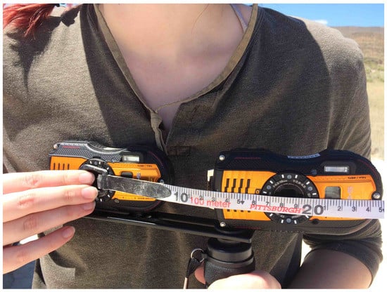
Figure 2.
Our camera set-up, mounted on the monopod.
To estimate the uncertainties in our stereogrammetry, we utilized the following geometric relationships, which we confirmed as accurate via preliminary experiments before the field campaign and from analyzing the campaign data. Take to be the angular distance between the feature of interest and the image center, given by
where x is the horizontal distance of the feature from the image center in pixels, the image’s horizontal field-of-view (71.5 for our cameras), and A the image width in pixels. Given a small uncertainty in the pixel position of a feature , we can estimate the angular uncertainty as
A typical pixel uncertainty few pixels translates into an angular uncertainty ≈0.1 mrad, meaning we are unable to measure parallax angles less than this value. It is important to keep in mind that these relationships hold for features near the center of the image plane, the situation most relevant for our study. Features far to the left or right of our observing station (i.e., along the line connecting our stereo cameras) will exhibit less parallax than suggested by this calculation. With a baseline of 0.18 m, for objects several meters distant, this parallactic uncertainty translates into an uncertainty in the radial distance of about 0.6 m. The parallactic uncertainty also means we are not able to measure distances larger than about m mrad ≈ 80 m. Unfortunately, as we discuss below, this limitation prevented us from accurately assessing distances during some of our dust devil encounters.
2.2. Pressure-Temperature Logger
To collect pressure time-series from onboard the drone, we used a commercially available logger, the B1100-1 by Gulf Coast Data Concepts (Waveland, MS 39576, USA), a sensor our group has used for previous dust devil studies [21]. The unit resembles a large USB flashdrive, and the whole assembly is about 2.5 cm in diameter and 10 cm long and weighs only 55 g with a battery installed, making it ideal for mounting on a drone with a limited payload capacity. The pressure time-series was collected at sampling rate of 2 Hz and a pressure resolution of 0.01 mb, adequate to detect typical dust devil pressure excursions of >1 mbar. The pressure sensor has a reported accuracy of ±0.15 hPa, but turbulent excursions during flight resulted in an effective uncertainty of about 0.3 hPa—see Section 3.2. The sensor registers pressure via an onboard transducer. Although the pressure time-series analyzed exhibit excursions resulting from the drone’s rotors and turbulent eddies (other than dust devils) during flight, we were largely successful in extracting the dust devil signals, as described in Section 3.2.
The logger unit also collects temperatures at a sampling rate of 0.7 Hz and has a reported accuracy of ±1 C. However, temperature excursions were expected to be of only a few degrees C with durations probably not much more than a second [14], so we did not expect to detect the devils in the temperature time-series, which seems borne out by post hoc inspection of the data. Thus, we do not include a temperature time-series analysis.
2.3. Drone
We used a commercially available 3DR Solo drone (Berkeley, CA, USA), a 1.5 kg quadcopter spanning about 46 cm from propeller to propeller diagonally across the body of the drone and standing about 25 cm off the ground. The drone has a maximum altitude of 100 m and a range of about 0.8 km, depending on conditions (the Federal Aviation Administration requires the drone pilot remain in visual contact). It has a payload capacity of 500 g and a maximum flight time on one battery of about 25 min. The drone is capable of flying in headwinds and crosswinds of about 11 m/s (25 miles-per-hour)—though some terrestrial dust devils exhibit windspeeds >11 m/s, tangential windspeeds for dust devils of a few m/s are more typical.
The drone provides a variety of real-time telemetry streams at 5 Hz sampling, in particular the aircraft attitude and GPS location and altitude, back to a hand-held controller where they are recorded. The drone also carries a 3-Axis gyro-stabilized gimbal and camera frame into which was mounted a GoPro 3 Silver (San Mateo, CA, USA). The video feed from this camera is piped into the drone itself and transmitted back to the controller from which it is fed into a smartphone, providing live video and audio from the perspective of the drone.
The drone is capable of self-directed flying between designated waypoints. However, since there were no pre-determined waypoints for our dust devil survey, we did not use the autopilot. We also deactivated the automated altitude hold, which relies on barometric measurements to estimate altitude. Since the dust devils exhibit low-pressure excursions, the drone would presumably have attempted to descend upon encountering a dust devil while in this mode.
3. Data Analysis
During several hours at our field site, we successfully launched the drone three times (Flights 0, 1, and 2) and had encounters with dust devils each launch. During Flight 0, we passed through the same dust devil twice. During Flight 1, we only knowingly encountered one dust devil, while, during Flight 2, we encountered two separate dust devils, with a short touchdown between the encounters. Our field campaign generated one pressure time-series from the B1100-1 logger, videos from the camera onboard the drone from each flight, and several pairs of photos and videos from the stereo camera set-up.
Regarding the imaging data from the stereo cameras, we employed different approaches throughout the field campaign, moving from synchronized still images to video imaging between different drone launches. Due to ineffective coordination between our team members, we were only able to recover stereo video for the dust devil encounter during Flight 1, although the limited parallactic baseline of 0.18 m made our stereo measurements difficult. The onboard drone video allowed us to recover the approximate timing of dust devil encounters during Flights 0 and 2.
3.1. Video Analysis
3.1.1. Analysis of the Drone Video
Figure 3 and Figure 4 show stills from the videos collected from the camera onboard the drone during Flights 0 and 2. The camera collected dust in the center of the frame, making the dark smudge. For an unknown reason, no video was collected during Flight 1. The Flight 0 video is available at [22], and the Flight 2 video at [23].
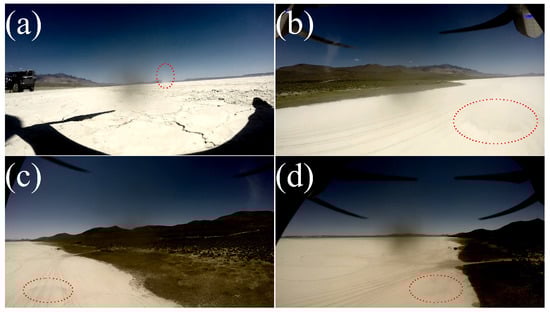
Figure 3.
Stills from the video collected onboard the drone during Flight 0. (a) just prior to launch (which occurred at approximately timestamp 0:31), with the first target dust devil highlighted by a red, dashed circle; (b) the dust skirt of the first target dust devil just prior to the first encounter, which occurred approximately 12 s after launch (at timestamp 0:43); (c) the dust skirt of the first dust devil just prior to the second encounter, which occurred approximately 23 s after launch (at timestamp 0:54); (d) the dust skirt of the second dust devil just prior to the first and only encounter, which occurred approximately 36 s after launch (at timestamp 1:07).
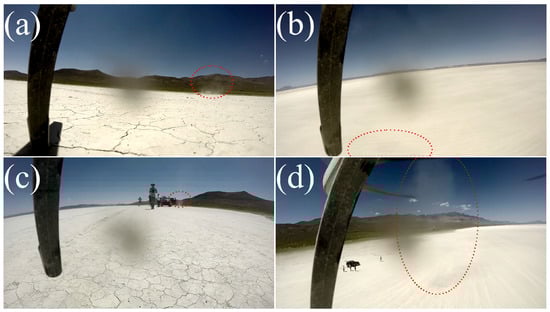
Figure 4.
Stills from the video collected onboard the drone during Flight 2. (a) just prior to launch (which occurred at approximately timestamp 0:14), with the first target dust devil highlighted by a red, dashed circle; (b) the dust skirt of the first target dust devil just prior to one encounter, which occurred approximately 22 s after launch (at timestamp 0:36); (c) the drone has nearly landed after encountering the first dust devil seen during Flight 2, but instead of landing, the drone ascended again to chase the dust devil highlighted to the right of the pilot; (d) just prior to the first encounter with the second dust devil seen during Flight 2 about 2 min after launch (timestamp 2:14).
To compare the videos to the other records, we first estimated the times at which the drone appeared to lift off the ground for each flight—approximately timestamp 0:31 for Flight 0 and timestamp 0:14 for Flight 2. These launch times are easily discernible in the pressure and altitude time-series analyzed below and so set the reference time against which the dust devil encounters are judged.
To more easily locate the dust devils in the footage, we significantly enhanced the video contrast. By recording the timestamp at which the drone appeared to pass over the skirt, we were able to estimate the approximate times of encounters, as indicated in the caption for Figure 3 and Figure 4.
As is apparent in the images, the dust skirts are difficult to discern in the videos (although their motion in the videos makes locating them a bit easier). In addition, as the drone passes over the skirt, it disappears from view. Together, these difficulties make our estimates of the encounter times uncertain to at least a few seconds but probably not much more. In any case, the purpose of this proof-of-concept study is only to explore the feasibility of this approach to probing dust devils, not to produce high precision measurements.
With these caveats in mind, we attempted to measure the diameters of the dust devils encountered from the drone videos. Using the still frames shown in Figure 3 and Figure 4, we located the horizontal pixel positions of the leftmost and rightmost edges of the dust skirts for each dust devil. We then applied Equation (3) to estimate their angular diameters. We made no effort to account for perspective effects or the fish-eye geometric distortion present within the GoPro camera that distorted the images of the devils and skew the diameter estimates.
To convert these angular diameters into physical diameters, we approximated the distances between the camera and devils as the drone’s altitude at the time of the still images. As described in Section 3.2 below, we can estimate the time of launch in the altitude time-series, set that time equal to the launch timestamp from the video, and then look up the drone’s altitude from the time-series at the time of encounter. Table 1 below shows our estimated diameters and, for the one devil we encountered more than once, the values from the different encounters are consistent, and all the diameters are qualitatively consistent with our impressions in the field of a few meters.

Table 1.
Dust devil diameters inferred from the video collected from onboard the drone.
Regarding Flight 2, the video and pressure time-series show some indication of an encounter with dust devil 1 about 8 s after launch (timestamp 0:22), but it is not entirely clear. Consequently, we do not include it as an encounter here and instead start with the encounter at 22 s after launch (at timestamp 0:36).
Regarding Flight 2, the dust skirt for the first dust devil was not visible from the air before the first encounter, and so instead, we measured the skirt’s diameter shortly after the encounter, approximately 38 s after launch at timestamp 0:49.
3.1.2. Analysis of the Stereo Videos Collected from the Ground
We also attempted to analyze the stereo video collected during Flight 1 from the ground, stills from which are shown in Figure 5. (The video is available at [24].) The left and right cameras were not turned on at precisely the same instant, so the videos are out of sync by about a second. To synchronize the videos, we compared their audio tracks. First, we converted the audio tracks from the videos into single-channel WAV files with a sampling rate of 44,000 Hz using ffmpeg [25]. To determine the delay between the videos, we performed a cross-correlation between the two audio tracks, using a distinctive, 10-s portion of the left camera’s track (co-author Davis says, “Perfect” during the dust devil encounter)—to reduce the computational time, we lowered the audio sampling rate to 440 Hz. This analysis suggested a delay of 1.2 s between the videos, and using this time shift, we trimmed both videos so they were very nearly synchronized.
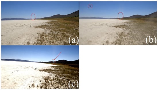
Figure 5.
Stills from the video collected by the left camera in the stereogrammetry set-up during Flight 1. (a) the first (and only) dust devil appears at a distance of about 80 m, approximately 20 s before launch (at timestamp 0:00); (b) the drone appears in frame and heads toward the dust devil, approximately 3 s after launch (at timestamp 0:23); (c) contrast-enhanced still of the approximate moment of encounter, when the lateral position of the drone (indicated by the red line) appears to coincide with the dust devil’s center, approximately 18 s after launch (at timestamp 0:38). An anemometer appears near the center of each image.
Although there do exist automated stereo analysis tools for video (OpenCV provides such capabilities, for example – [26]), preliminary experimentation suggests they require better controlled stereo data than we have and more distinctive features than dust devils to work effectively. Thus, instead of an automated analysis, we opted to conduct the stereo analysis by hand. To keep the analysis manageable, we collected still frames from each video using OpenCV, one per second. By comparing the horizon in the images to satellite imagery from Landsat (Figure 1), we estimated that the distant peaks (Figure 1) near the center of each frame (Figure 5) are approximately 17 km away, distant enough that they should exhibit no measurable parallax between our stereo cameras. Thus, we used the rightmost peak as an anchor point for our stereo analysis, measured the pixel offset, and there from the angle (Equation (3)), for each feature of interest relative to that peak. With this angle measured for each feature of interest in the left () and right () frames, we estimated the distance to the feature , where b is the baseline between the cameras.
As a control, we estimated the distance to the anemometer (Figure 5) and found m, consistent with our field measurements. When we attempted to estimate the distance to dust devil 1 encountered during Flight 1, for several of the still images, we found a distance of roughly 80 m, which is consistent with the apparent encounter timing for the drone (see Section 3.2), but, for several other images, the distance estimates were inconsistent. Given the difficulty of locating the dust devil in the images, it is likely that, as strands of dust swept in and out of view over the course of the dust devil’s travel, the apparent center of the devil shifted by a few pixels, giving rise to the inconsistent distances measured. In Section 4, we discuss future strategies to improve upon the approach here, but we were able to estimate the approximate time of encounter for Flight 1 by determining when the lateral positions of the drone and dust devil coincided—18 s after launch at a timestamp of 0:38—which is consistent with our estimate from the time-series (Section 3.2). Assuming a distance of 80 m, we estimated the dust devil’s diameter as approximately 1.8 m.
3.2. Pressure and Altitude Time-Series Analysis
In this section, we describe our analysis of the pressure time-series. As discussed below, we employed perhaps a more sophisticated analysis approach than merited by the available data because this study serves as preparation for larger follow-on studies, during which we expect to collect considerably more and higher quality data.
Figure 6 shows the pressure time-series collected by the logger attached to the drone, along with the drone’s altitude as determined by the onboard GPS unit. The drone launches are apparent in both time-series: in the pressure log as dips bracketed by spikes (due to the propellers’ ground effect) and in the altitude as sudden increases. The pressure log also shows a discernible, if subtle, downward trend, tracking the diurnal decrease in pressure as the boundary layer is heated. To remove this long-term linear trend, we simply masked out the launches from the pressure time-series and fit a linear trend to the resulting data.
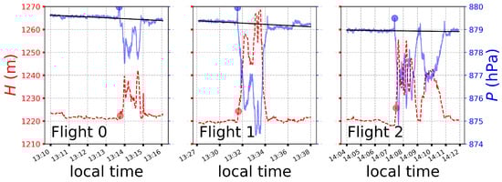
Figure 6.
Altitude H in meters (red, dashed line) and pressure P in hPa (blue, solid line) vs. local time. The solid black line shows a linear trend, with the flights (upward excursions in altitude and downward excursions in pressure) masked out. The red and blue dots represent the estimated launch times.
Having subtracted the linear trend, we next interpolated the GPS altitude time-series to the times of the pressure data since they were sampled at different rates (GPS at 20-Hz, pressure at 2-Hz). Since they are recorded by two unsynchronized instruments, the altitude and pressure time-series are offset by many seconds. To estimate the exact timing offset, we cross-correlated the two time-series (interpolated to the same timestamps) and looked for the minimum (since pressure and altitude should be anti-correlated, modulo the dust devil signals), which occurs at a time-shift of 21.04 s.
For comparison to the drone video, we estimated the instant of launch as reflected by the pressure and altitude time-series. For the pressure time-series, we took the launch to coincide with the maximum that occurs just prior to the pressure drop corresponding to the drone’s ascent. The altitude time-series exhibits pre-launch variations of about 0.5 m, making a determination of the exact instant of launch (i.e., the time when altitude steadily increases) somewhat uncertain.
To address this uncertainty and as a check on the launch-time estimate from the pressure time-series, we implemented a change-point analysis using the Bayesian Blocks algorithm [27]. Briefly, this scheme attempts to optimally segment a time-series into a sequence of constant values of possibly variable durations (i.e., each block can span a different length of time). It minimizes the variation within each block, while, at the same time, implementing a penalty in the form of Bayesian prior as the number of blocks increases. This approach threads the needle between capturing variability in the time-series without including too much noise, and the boundaries between the blocks represent the statistically significant change points—in our case, the launch time. Figure 6 illustrates the launch times as colored dots. Based on the figure, the pressure launch times seem to be a better representation of the correct values, so we use those in the subsequent analyses.
Next, we looked for the signals from the dust devils. The pressure signals during flight are dominated by the hydrostatic drop/increase in pressure as the drone ascends/descends, potentially masking the small, negative excursions due to dust devil encounters. Since the atmospheric pressure scale height (8 km) is much larger than the drone’s maximum altitude (≤100 m), we approximated the pressure–altitude relationship as linear and applied and subtracted a linear regression to the pressure vs. altitude data (Figure 7), leaving the residual pressure signals shown in Figure 8. Although the drone’s rotors do influence the pressure log during take-off and landing, the fact that the pressure and altitude are so strongly correlated during flight suggests the rotors do not otherwise significantly distort or contribute to the pressure time-series, meaning they are probably not responsible for any of the dust devil-like signals we identify below.
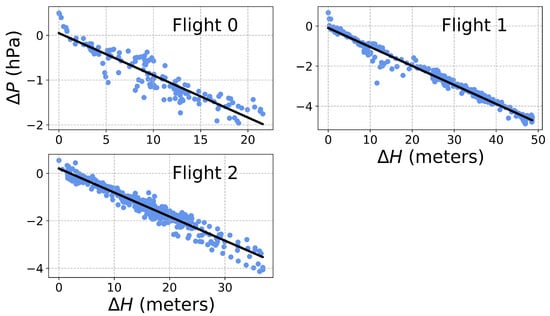
Figure 7.
Pressure vs. altitude for the three flights from Figure 6. The black lines show linear fits for each launch.
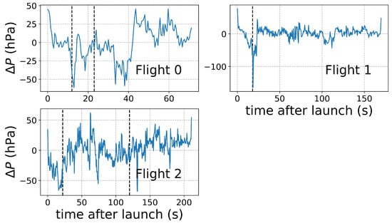
Figure 8.
Pressure residuals after removing the linear, hydrostatic trends shown in Figure 7. The dashed, black vertical lines represent the approximate dust devil encounter times estimated from the video data (Section 3.1).
We next attempted to fit pressure profiles to the apparent dust devil signals in these residual pressure time-series. As discussed in Section 1, a dust devil’s radial structure is commonly represented by a Lorentz profile—for a simple, linear trajectory through the dust devil (which we assumed), the signal in time will also be a Lorentz profile. However, the residual pressure time-series for all three flights show considerable variability, probably due to turbulent excursions and instrument noise and not to dust devil encounters. Since these excursions exhibit coherent structure over several seconds, they represent non-white noise, and so accurately fitting pressure profiles during the dust devil encounters requires incorporating a more complex noise model. It is worth pointing out that the encounter timing constraints play a key role here since they tell us where in the pressure time-series to look for the devils. Without these constraints, we might struggle to distinguish pressure excursions due to dust devils from other turbulent signals.
For our study, we chose to model the pressure time-series using a Gaussian processes (GP) approach [28,29]. In contrast to the usual white noise model under which the point-to-point scatter is assumed to be uncorrelated, the GP model allows the scatter at one point to depend on the scatter for nearby points. In other words, the covariance matrix has non-zero off-diagonal elements, and the GP approach fits a model kernel to the elements of that matrix—in our case, we assumed a Matern-3/2 kernel [28]. To fully and efficiently sample the space of model fit parameters for the dust devil profile, , (see Equation (1)), and the central encounter time , we also employed the affine-invariant Markov-Chain Monte-Carlo (MCMC) scheme described in Goodman and Weare [30] and implemented in Foreman-Mackey et al. [31], which provides us with an effective posterior distribution for the model parameters. For comparison, we also fit the pressure data using a more traditional white noise model and the Levenberg–Marquardt (LM) scheme, e.g., [32], taking the uncertainties on fit parameters as the square root of the covariance matrix.
To begin, since it exhibits the clearest dust devil signal, we first considered the pressure time-series for Flight 1 (rightmost panel in Figure 5) (and considered just the first 50 s of the time-series to reduce the computational time, which scales with the third power of the number of data points). Figure 9 shows the results: the leftmost panel shows the model fit using the Gaussian processes approach (solid, red lines) and using the LM approach (dashed, blue). (It is important to note that the red curves represent several instantiations of the noise model for the data since the Gaussian processes approach does not solve directly for the noise, just the covariance function nuisance parameters.) For the MCMC sampler, we used 32 walkers and employed two burn-in phases, each with at least 1000 steps and a final production run of at least 2000 steps, which resulted in converged chains with acceptance fractions between 25% and 50%, cf. [33].
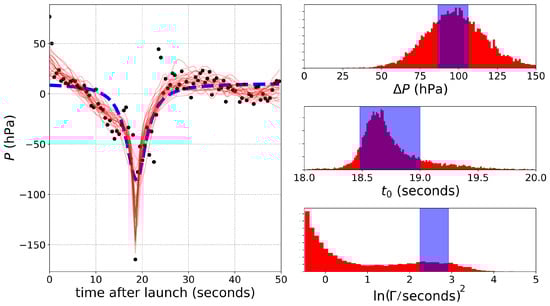
Figure 9.
Model fits and parameters for the pressure residuals from Flight 1 (i.e., from Figure 8). The left panel shows two model fits to the dust devil 1 encounter—the best-fit model shown by the dashed, blue line assumes white noise and uses the Levenberg–Marquardt fitting routine but does not illustrate the noise at all (i.e., does not include any scatter in the line). The solid, red lines show fits assuming a Gaussian processes noise model and a Markov Chain Monte Carlo (MCMC) parameter space sampling and includes several estimates of the noise signal—hence the waviness. The right panels show the best-fit parameters—shaded blue, the 1- uncertainties for the former modeling scheme, and red, the distributions from the MCMC chains.
The right panels show the distribution of best-fit parameters—the red histogram, from the GP-MCMC analysis, and the blue shaded region, the 1- uncertainties from the white noise-LM analysis. (We fit for rather than to keep the solution numerically well-behaved.) The two approaches return nearly the same profile depth and center but very different profile widths : the best-fit LM value is s, compared to the mode in the MCMC distribution s, which suggests the turbulent excursions in the data fool the LM analysis into choosing a much wider profile. Indeed, the video footage suggested a dust devil only 1.8 m in diameter (Section 3.1.2). During the encounter, the drone has a velocity of about 5 m/s, and, with a logger sampling rate of 2 Hz, we would not expect more than one point in the profile (assuming the visible diameter corresponds to the profile width). A 3.6-s-wide profile would correspond to an 18-m dust devil.
We then applied the MCMC-GP approach to modeling the pressure time-series for Flights 0 and 2 (we did not include the LM analysis). For the Flight 0 encounters, we fit two Lorentz profiles simultaneously since the encounters were very close in time, while, for the Flight 2 encounters, we broke the time-series into two parts. Figure 10, Figure 11 and Figure 12 show the results. In contrast to the Flight 1 encounter, these encounters are less distinct, as reflected in the distributions of best-fit parameters. During the two encounters, the drone again had a ground-speed of about 5 m/s, and given the apparent dust devil diameters (Table 1), the encounters should have durations of about 1 s, consistent with the mode of the distributions shown in Figure 10.
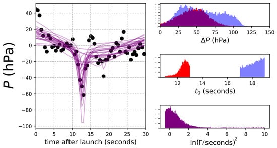
Figure 10.
The left panel shows the two-Lorentz profile fits to the pressure time-series from Flight 0. The right panels show the best-fit parameters for the two Lorentz profiles—the red histograms for the earlier encounter, the blue, for the later.
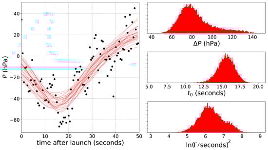
Figure 11.
The left panel shows the Lorentz profile fit to first part of the pressure time-series from Flight 2. The right panels show the best-fit parameters for profiles.
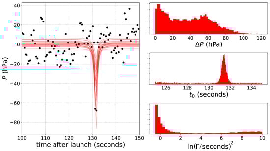
Figure 12.
The left panel shows the Lorentz profile fit to a later part of the pressure time-series from Flight 2. The right panels show the best-fit parameters for profiles.
The Flight 2 encounters (Figure 11 and Figure 12) also do not register as distinctly as the encounter from Flight 1. The first encounter from Flight 2 (Figure 11) has a definite non-zero -value; however, that dust devil seems to have been lost in the longer-term variability in the time-series—the best-fit -value corresponds to a profile width of nearly 50 s. There are two significant outliers registering the second encounter (Figure 12); however, the dust devil’s profile is not otherwise resolved, which is why the distribution of -values (top, right panel) exhibits a non-negligible peak near zero (i.e., no signal). During the encounter, the drone had a ground speed of about 7 m/s, meaning the 2-m wide devil might register as a single data point.
4. Discussion
Our pilot study has shown the potential of using an instrumented drone to probe the structure of active dust devils. In the four dust devil encounters cataloged here, we recovered pressure signals roughly consistent with the devils’ structures as inferred from the visual data. However, the study also suggested several improvements that would significantly bolster the results.
Foremore, improved collection of location data (drone and dust devil) is critical. For example, markers placed in the field would help locate the dust devil, and a real-time kinematic navigation system would help with the drone. Another limitation of the current study is our inability to robustly corroborate the sizes of the encountered dust devils and to determine the timing of the encounters from the stereo imagery. For future studies, we plan to collect video of each encounter. Assuming we use the Ricoh WG-5 GPS cameras again, we could resolve angles down to a few 0.1 (Equation (4)). To estimate their diameters from the imagery data, we would need to resolve them with several (∼10) pixels, meaning they must be near enough to subtend at least 1 (≈0.02 rad). If we again encountered dust devils with diameters of a few meters, the cameras’ angular resolution would limit us to encounters no more distant than 150 m (≈3 m/2 rad). At this distance, we would require a parallactic baseline of at least 3 m. However, our pilot had a fair amount of difficulty visually resolving the encounter during Flight 1 with a devil at 80-m distance, suggesting that this distance is a more reasonable maximum, allowing a baseline of 1.5 m, which would facilitate the use of the commercially available Ricoh WG-5 GPS remote control. A lidar system would also be well suited for dust devil studies, and, indeed, has been used in limited previous work [34]. Recently, Shiina et al. [35] described development of a miniature, low-power LED lidar, designed for use on a Mars lander where power limitations can be considerable.
The next most important improvements would be to enhance the instrumentation and data collection on the drone. For instance, the low sampling rate (2 Hz) used for the pressure logger in this pilot study prevented us from fully resolving the devils’ pressure structure. Fortunately, the most recent version of the logger, the B1100-2, allows sampling at 20 Hz, sufficient to resolve a few-meter dust devil encountered at 5 m/s with several data points. With its payload capacity, the 3DR Solo could easily carry additional instruments. In particular, a particle collector, if small enough and capable of high-time-resolution sampling, would prove especially useful for assessing devil dust-lifting capacities. A combination of video analysis and remote lidar measurements might also be well suited to assessing dust column densities. Including a fast response temperature sensor in the payload package would also substantially facilitate mapping structures within dust devils and testing the expected thermodynamic relationships.
A more complete assessment of the microscale meteorological environment might also substantially enhance the return from a drone study such as ours. Previous work suggests dust devils form at the corners between large (∼100 m) eddy structures in the boundary layer (see references in [36]). In addition, the height and vigor of a dust devil seem to scale with the depth of the boundary layer [37]. A drone dust devil survey could be accompanied by deployment of a small array of meteorological instrumentation—pressure loggers to map convective cells and anemometers to follow their advection, along with atmospheric sounding equipment to measure boundary layer depth—to map conditions around an active dust devil and test model predictions and previous observations.
Acknowledgments
This work was supported in part by the Idaho Space Grant Consortium. Ralph Lorenz acknowledges support from NASA’s Mars Fundamental Research Program grant NNX12AI04G. This work was facilitated by Bradley Ward. We also gratefully acknowledge detailed feedback from anonymous referees.
Author Contributions
B.J. and R.L. conceived and designed the experiments. All authors participated in performing the experiments. B.J. analyzed the data, and all authors contributed to writing the paper.
Conflicts of Interest
The authors declare no conflicts of interest.
References
- Gillette, D.A.; Sinclair, P.C. Estimation of suspension of alkaline material by dust devils in the United States. Atmos. Environ. 1990, 24, 1135–1142. [Google Scholar] [CrossRef]
- Lorenz, R.; Myers, M. Dust Devil Hazard to Aviation: A Review of United States Air Accident Reports. J. Meteorol. 2005, 30, 178–184. [Google Scholar]
- Balme, M.; Greeley, R. Dust devils on Earth and Mars. Rev. Geophys. 2006, 44. [Google Scholar] [CrossRef]
- Lorenz, R.; Reiss, D. Solar Panel Clearing Events, Dust Devil Tracks, and in situ Vortex Detections on Mars. Icarus 2014, 248, 162–164. [Google Scholar] [CrossRef]
- Cantor, B.A. MOC observations of the 2001 Mars planet-encircling dust storm. Icarus 2007, 186, 60–96. [Google Scholar] [CrossRef]
- Shirley, J.H. Solar System dynamics and global-scale dust storms on Mars. Icarus 2015, 251, 128–144. [Google Scholar] [CrossRef]
- Smith, M.D. Interannual variability in TES atmospheric observations of Mars during 1999–2003. Icarus 2004, 167, 148–165. [Google Scholar] [CrossRef]
- Basu, S.; Richardson, M.I.; Wilson, R.J. Simulation of the Martian dust cycle with the GFDL Mars GCM. J. Geophys. Res. Planets 2004, 109. [Google Scholar] [CrossRef]
- Neakrase, L.D.V.; Greeley, R. Dust devil sediment flux on Earth and Mars: Laboratory simulations. Icarus 2010, 206, 306–318. [Google Scholar] [CrossRef]
- Neakrase, L.D.V.; Balme, M.R.; Esposito, F.; Kelling, T.; Klose, M.; Kok, J.F.; Marticorena, B.; Merrison, J.; Patel, M.; Wurm, G. Particle Lifting Processes in Dust Devils. Space Sci. Rev. 2016, 203, 347–376. [Google Scholar] [CrossRef]
- Rennó, N.O.; Burkett, M.L.; Larkin, M.P. A Simple Thermodynamical Theory for Dust Devils. J. Atmos. Sci. 1998, 55, 3244–3252. [Google Scholar] [CrossRef]
- Ryan, J.A.; Carroll, J.J. Dust devil wind velocities: Mature state. J. Geophys. Res. 1970, 75, 531–541. [Google Scholar] [CrossRef]
- Kurgansky, M.V.; Lorenz, R.D.; Renno, N.O.; Takemi, T.; Gu, Z.; Wei, W. Dust Devil Steady-State Structure from a Fluid Dynamics Perspective. Space Sci. Rev. 2016, 203, 209–244. [Google Scholar] [CrossRef]
- Rennó, N.O.; Nash, A.A.; Lunine, J.; Murphy, J. Martian and terrestrial dust devils: Test of a scaling theory using Pathfinder data. J. Geophys. Res. 2000, 105, 1859–1866. [Google Scholar] [CrossRef]
- Lorenz, R.D.; Neakrase, L.D.; Anderson, J.D. In-situ measurement of dust devil activity at La Jornada Experimental Range, New Mexico, USA. Aeolian Res. 2015, 19, 183–194. [Google Scholar] [CrossRef]
- Jackson, B.; Lorenz, R.; Davis, K. A framework for relating the structures and recovery statistics in pressure time-series surveys for dust devils. Icarus 2018, arXiv:astro-ph.EP/1708.00484299, 166–174. [Google Scholar] [CrossRef]
- Lorenz, R. The longevity and aspect ratio of dust devils: Effects on detection efficiencies and comparison of landed and orbital imaging at Mars. Icarus 2013, 226, 964–970. [Google Scholar] [CrossRef]
- Sinclair, P.C. The Lower Structure of Dust Devils. J. Atmos. Sci. 1973, 30, 1599–1619. [Google Scholar] [CrossRef]
- Metzger, S.M.; Balme, M.R.; Towner, M.C.; Bos, B.J.; Ringrose, T.J.; Patel, M.R. In situ measurements of particle load and transport in dust devils. Icarus 2011, 214, 766–772. [Google Scholar] [CrossRef]
- Sinclair, P.C. A Quantitative Analysis of the Dust Devil. Ph.D. Thesis, The University of Arizona, Tucson, AZ, USA, 1966. [Google Scholar]
- Lorenz, R.D. Observing desert dust devils with a pressure logger. Geosci. Instrum. Methods Data Syst. Discuss. 2012, 2, 477–505. [Google Scholar] [CrossRef]
- YouTube. Available online: youtu.be/MAdwmv8yRgs (accessed on 4 January 2018).
- YouTube. Available online: youtu.be/9VtcSrBjflY (accessed on 4 January 2018).
- YouTube. Available online: youtu.be/Rj7wua4GQyc (accessed on 4 January 2018).
- ffmpeg. Available online: https://www.ffmpeg.org/ (accessed on 4 January 2018).
- opencv. Available online: http://opencv.org/ (accessed on 4 January 2018).
- Scargle, J.D.; Norris, J.P.; Jackson, B.; Chiang, J. Studies in Astronomical Time Series Analysis. VI. Bayesian Block Representations. Astrophys. J. 2013, arXiv:astro-ph.IM/1207.5578764, 167. [Google Scholar] [CrossRef]
- Rasmussen, C.E.; Williams, C.K.I. Gaussian Processes for Machine Learning; University Press Group Limited: Bognor Regis, UK, 2006. [Google Scholar]
- Ambikasaran, S.; Foreman-Mackey, D.; Greengard, L.; Hogg, D.W.; O’Neil, M. Fast Direct Methods for Gaussian Processes. ArXiv, 2014; arXiv:math.NA/1403.6015. [Google Scholar]
- Goodman, J.; Weare, J. Ensemble samplers with affine invariance. Commun. Appl. Math. Comput. Sci. 2010, 5, 65–80. [Google Scholar] [CrossRef]
- Foreman-Mackey, D.; Hogg, D.W.; Lang, D.; Goodman, J. emcee: The MCMC Hammer. Publ. Astron. Soc. Pac. 2013, arXiv:astro-ph.IM/1202.3665125, 306. [Google Scholar] [CrossRef]
- Press, W.H.; Teukolsky, S.A.; Vetterling, W.T.; Flannery, B.P. Numerical Recipes in C++ : The Art of Scientific Computing; Cambridge University Press: Cambridge, UK, 2002. [Google Scholar]
- Ford, E.B. Improving the Efficiency of Markov Chain Monte Carlo for Analyzing the Orbits of Extrasolar Planets. Astrophys. J. 2006, arXiv:astro-ph/0512634642, 505–522. [Google Scholar] [CrossRef]
- Renno, N.O.; Abreu, V.J.; Koch, J.; Smith, P.H.; Hartogensis, O.K.; De Bruin, H.A.R.; Burose, D.; Delory, G.T.; Farrell, W.M.; Watts, C.J.; et al. MATADOR 2002: A pilot field experiment on convective plumes and dust devils. J. Geophys. Res. Planets 2004, 109, E07001. [Google Scholar] [CrossRef]
- Shiina, T.; Yamada, S.; Senshu, H.; Otobe, N.; Hashimoto, G.; Kawabata, Y. LED minilidar for Mars rover. Proc. SPIE 2016. [Google Scholar] [CrossRef]
- Spiga, A.; Barth, E.; Gu, Z.; Hoffmann, F.; Ito, J.; Jemmett-Smith, B.; Klose, M.; Nishizawa, S.; Raasch, S.; Rafkin, S.; et al. Large-Eddy Simulations of Dust Devils and Convective Vortices. Sol. Syst. Rev. 2016, 203, 245–275. [Google Scholar] [CrossRef]
- Fenton, L.K.; Lorenz, R. Dust devil height and spacing with relation to the Martian planetary boundary layer thickness. Icarus 2015, 260, 246–262. [Google Scholar] [CrossRef]
© 2018 by the authors. Licensee MDPI, Basel, Switzerland. This article is an open access article distributed under the terms and conditions of the Creative Commons Attribution (CC BY) license (http://creativecommons.org/licenses/by/4.0/).