Edge Dependent Chinese Restaurant Process for Very High Resolution (VHR) Satellite Image Over-Segmentation

Beijing Key Laboratory of Environmental Remote Sensing and Digital Cities, Faculty of Geographical Science, Beijing Normal University, Beijing 100875, China
*
Author to whom correspondence should be addressed.
Remote Sens. 2018, 10(10), 1519; https://doi.org/10.3390/rs10101519
Submission received: 15 August 2018
/
Revised: 14 September 2018
/
Accepted: 18 September 2018
/
Published: 21 September 2018
(This article belongs to the Special Issue Image Segmentation for Environmental Monitoring)
Abstract
:Image over-segmentation aims to partition an image into spatially adjacent and spectrally homogeneous regions. It could reduce the complexity of image representation and enhance the efficiency of subsequent image processing. Previously, many methods for image over-segmentation have been proposed, but almost of them need to assign model parameters in advance, e.g., the number of segments. In this paper, a nonparametric clustering model is employed to the over-segmentation of Very High Resolution (VHR) satellite images, in which the number of segments can automatically be inferred from the observed data. The proposed model is called the Edge Dependent Chinese restaurant process (EDCRP), which extends the distance dependent Chinese restaurant process to make full use of local image structure information, i.e., edges. Experimental results show that the presented methods outperform state of the art methods for image over-segmentation in terms of both metrics based direct evaluation and classification based indirect evaluation.
1. Introduction
With the development of imaging techniques and the space satellite manufacturing, both spectral and spatial resolutions of Very High Resolution (VHR) satellite images have been improved significantly [1,2,3]. Consequently, VHR satellite images have been extensively applied to many applications, such as natural disaster monitoring [4,5], land cover change detection [6,7], environmental protection [8], and agricultural production [9], and so on [10,11]. Along with the increase in spatial resolution, it has becomes a considerable challenge for traditional methods to extraction information from VHR satellite images. Image over-segmentation is a common way to simplify image representations and speed image processing, by partitioning images into spatially adjacent and spectrally homogeneous regions [12,13].
Image over-segmentation has been widely used in many applications, including computer vision [14,15], object recognition [16,17], image retrieval [18,19], and image classification [20,21]. The following properties might be expected for a “good” over-segmentation result: (1) pixels within an segment should be spatially adjacent and have similar features; (2) the boundaries of segments should adhere well to the “meaningful” image boundaries; and, (3) each segment resides within only one real geo-object. Many over-segmentation algorithms have been used to segment everyday photos and pictures, and they aimed to achieve abovementioned properties, including the Simple Linear Iterative Clustering (SLIC) [22], Entropy Rate Superpixel segmentation (ERS) [23], normalized cut (NC) [24], edge-augmented mean-shift (ED) [25], and so on [26,27]. These methods can be roughly divided into four categories, including threshold-based algorithms [28,29], edge-based algorithms [30,31], graph-based algorithms [32,33], and clustering-based methods [34,35]. It is rather simple and efficient for the threshold-based algorithms to obtain over-segmentation from images. However, it is very difficult to choose the appropriate threshold. Although the boundary recall is often rather high in the results of edge-based methods, the results are often sensitive to the quality of the detected edges. It is straightforward for the graph-based algorithms to utilize the spatial constraints by measuring the affinity in terms of spectral or structural similarity.
Clustering-based methods are widely used for image over-segmentation by embedding spatial information. The SLIC is the most typical method to over-segmentation by clustering [22]. The Entropy Rate Superpixel (ERS) also treats the over-segmentation as a clustering problem [23]. The main difficulty for clustering-based methods to image segmentation is how to estimate the suitable number of clusters before clustering. As a Bayesian nonparametric clustering model, the Chinese restaurant process (CRP) mixture model [36], and its variants provide a principled way to infer the number of clusters from the observed data. An underlining assumption of these nonparametric clustering models is that the observed data in each group is modeled as an exchangeable sequence of random variables. In order words, for an exchangeable sequence of random variables, any permutation of the sequence has the same joint probability distribution as the original sequence [37]. If the CRP is directly applied to image clustering, the spatial dependency among pixels would be lost. Generally speaking, there exist three kinds of ways enhance spatial dependency among pixels when the CRP and its variants are applied to image analysis, i.e., preprocessing, poster-processing, and directly modeling the interdependence among neighboring variables [36]. For example, by using over-segmentation of VHR satellite images as a preprocessing, the CRP and its variants have been successfully applied to image or feature fusion [38], geo-object category detection [39], and unsupervised classification [40], and so on. However, it is difficult for humans to assign an appropriate number of over-segments, since a large number of geo-objects with different size and shapes are scattered in VHR satellite images without uniform spatial distribution. Majority voting using neighboring pixels are often used as a poster-processing to enhance spatial consistence of clustering labels [41]. However, the clustering results would be strongly dependent on both the presented neighboring system.
As an extension of the CRP, the distance dependent Chinese restaurant process (ddCRP) explicitly models the dependency between two random variables as a function of their distance [37]. The ddCRP was originally proposed for text modeling [37]. Whether and how can the ddCRP be effectively used for the over-segmentation of VHR satellite images? To answer this question, we systematically analyzed characteristics of the ddCRP. Specifically, we evaluated the impact of three components in the ddCRP model on the over-segmentation of VHR satellite images in this paper, i.e., the distance dependent term, the sampling probability term and the connection mode. Furthermore, we present an improved model for over-segmentation of VHR satellite images, which is termed as the Edge Dependent Chinese Restaurant Process (EDCRP).
The rest of this paper is organized as follows. In Section 2, we described the basic principle of the ddCRP, and analyzed the characteristics of its components. The EDCRP model was described in Section 3. Experimental results coupled with related discussions are given in Section 4. Some conclusions are drawn in Section 5.
2. Distance Dependent Chinese Restaurant Process
After the ddCRP is introduced in the first subsection, we systematically the characteristics of its three components, i.e., distance dependent term, likelihood term, and connection mode.
2.1. ddCRP
The CRP is a classical representation of the Dirichlet Process (DP) mixture model, which is an intuitional way to obtain a distribution over infinite partitions of the integers. Under the metaphor of the CRP, the random process is described, as follows. Customers enter a Chinese restaurant one by one for dinner. When a customer enters the restaurant, he or she chooses a table, which has been occupied by other customers who entered previously with a probability proportional to the number of customers already sitting at the table. Otherwise, one takes a seat at a new table with a probability proportional to a scale parameter . The random process is given by
where represents the index of table chosen by the customer; denotes the table assignments of N customers with the exception of customer; is the number of tables already occupied by some customers; and, denotes the number of customers sitting at table .
After all of the customers have taken their seats, a random partition has been realized. Customers sitting at the same table belong to a same cluster. This specific clustering property indicates a powerful probabilistic clustering method. The most important advantage of this algorithm is that the number of partitions does not need to be assigned in advance. The reason is that the CRP treats the number of clusters as a random variable that can be inferred from the observations by marginalizing out the random measure function.
Please note that, although the customers are described as entering the restaurant one by one in order, any permutation of their ordering has the same joint probability distribution of the original sequence. This is the exchangeability property of CRP mixture model. In practice, exchangeability is not a reasonable assumption for many realistic applications. As for image over-segmentation, it is necessary to identify the spatially contiguous segments where the same label is allocated to the neighbor pixels with homogeneous spectra. Therefore, the traditional CRP model is not suitable for image over-segmentation. To introduce the dependency among random variables, Blei et al. proposed the distance dependent Chinese restaurant process (ddCRP) in [37]. The partition, formed by assigning the customers to tables in the CRP, is replaced with the relationship between one customer and other customers in the ddCRP. Under the similar metaphor of the CRP, the ddCRP model states that each customer selects another customer to sit with, who has already entered the restaurant. Given the relationship among customers, it is easy to infer which customers will sit at the same table. Therefore, the tables are a byproduct of the customer assignments. Let denote the decay function, the distance measure between two observations and , the scaling parameter, and the customer assignment of customer, i.e., customer choose to sit with customer. The random process is to allocate customer assignments according to
where the distance measure is used to evaluate the difference between the two observations i and j, and the decay function mediates how the distance affects the probability of connecting the two customers together. The farther the distance between the two data points, the smaller their probability of connecting with each other. The traditional CRP is a particular case of ddCRP when the decay function is assumed to be a constant, i.e., .
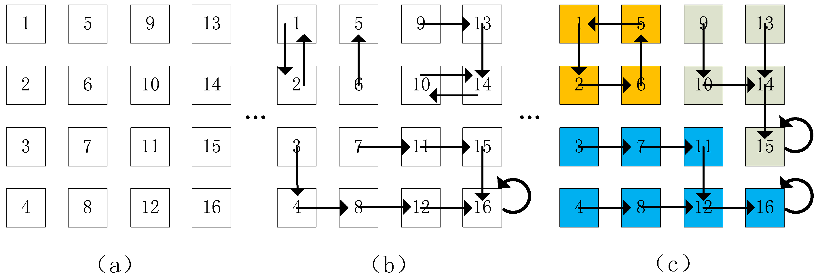
To bridge the gap of terminologies between feature clustering and image over-segmentation, Figure 1 is employed to construct the analogy between the metaphor of ddCRP and image over-segmentation. An image with 16 pixels is shown in Figure 1a, where each numbered square denotes a pixel. The image is a restaurant, which accommodates 16 customers under the metaphor of the ddCRP. Figure 1b shows a middle state during the random process of customer assignments, where each arrow indicates a customer choose to sit with another customer. All of customers, who chose to sit with, naturally form a cluster. In other words, they sit at a same table in the ddCRP. This is illustrated in Figure 1c, where the pixels with a same color belong to a cluster. Under the terminology of image over-segmentation, a segment also consists of all of the pixels with a same color, where every two pixels within a segment can reach to each other along the inferred customer assignments in the ddCRP. Therefore, the inferred customer assignments are the key to derive the results of image over-segmentation.
Given an image with N pixels , the image over-segmentation is to partition pixels into multiple regions with label . In the ddCRP, the label is a by-product of customer assignment , whose posterior is given by . The customer assignment, e.g., , is assumed to be dependent on the distance between two pixels, e.g., and is independent of other customer assignments. Therefore, the posterior of customer assignment is proportional to
where the likelihood of image pixels is given by . It is difficult to compute the posterior because the ddCRP places a prior over a huge number of customer assignments. A simple Gibbs sampling method can be used to approximate the posterior by inferring its conditional probability
where represent the customer assignments of all of the pixels with exception of pixel, and denotes the pixels associate with segment derived from ; is a prior of the parameter , which is utilized to generate observations using a probability . In this paper, the prior and the probability distribution are assumed to be Dirichlet process [36] and multinomial distribution, respectively. The parameter can be marginalized out, since they are conjugated. As a family of stochastic processes, the Dirichlet process can be seen as the infinite-dimensional generalization of the Dirichlet distribution.
As the shown in Equation (4), there are three possible situations to generate a new assignment . In situation 1, the assignment points to another pixel but do not make any change in the over-segmentation result. The situation 2 means that two different segments are merged into a new segment due to the customer assignment . For situation 3, the assignment points to itself in a probability proportional to .
In the following, we analyze the characteristics of the three components in the ddCRP, i.e., the distance dependent term , the likelihood of the image , and the connection mode among the pixels.
2.2. Distance Dependent Term
As for image over-segmentation, the dependence between the pixels can be naturally embedded into the ddCRP by the use of a spatial distance measure and a decay function, for example, the Euclidean distance between pixels where is pixel’s location in an image. The decay function is used to mediate the effects of distance between pixels on the sampling probability. The decay function should satisfy the following nonrestrictive assumptions; it should (1) be nonincreasing and (2) take nonnegative finite values, and (3) . There are several types of decay functions [37], such as the window decay function, the exponential decay function and the logistic decay function. If the distance satisfies the preference, the decay function returns a larger value; otherwise, it returned a smaller value.
Since over-segments consist of a set of pixels that are spatially adjacent and spectrally homogeneous, only the neighboring pixels are considered in this paper, i.e., pixels and with spatial distance . As shown in Figure 1, the possible assignments of the 11th pixel consist of 7th, 10th, 12th, and 15th pixels. Therefore, the information on neighboring spatial locations has been introduced by this setting. In order to take spectral information between neighboring pixels into account in this model, the spectral difference between neighboring pixels is also introduced in the ddCRP. Spectral distance can be represented by the difference , where is the DN value of i-th pixel. So, the spectral difference and the spatial distance are combined to the final distance measure, . The ddCRP model with spatial and spectral distance abbreviated to spatial-spectral ddCRP model. In our previse work [42], empirical experiments showed that the spatial-spectral ddCRP model exhibits a promising performance.
2.3. Likelihood Term
Let the prior and probability distribution are the Dirichlet distribution and the multinomial distribution, respectively. Given customer assignments , the likelihood of kth segment is
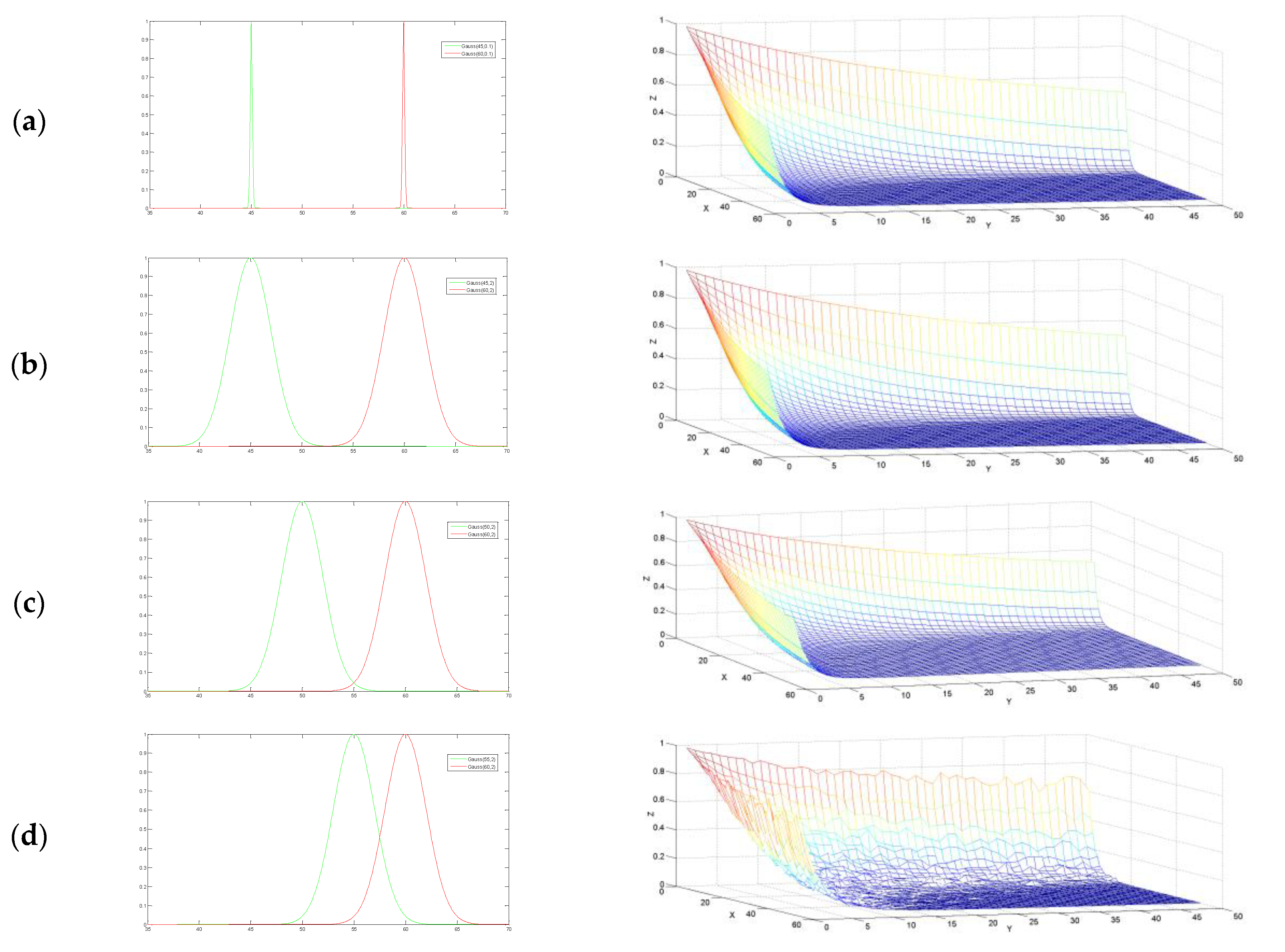
where denotes the parameter of the base distribution , which is initialized while using a uniform distribution. The represents the gamma function. Each visual word is denoted by . In this paper, the visual word is a digital number (DN) value of panchromatic images. denotes the number of pixels belonging to the segment. As shown in Equation (2), kth and lth over-segments could be merged into a new one in a probability proportional to the production of distance dependent term and the likelihood ratio . For the sake of simplifying description, the likelihood ratio is called the merging probability of two over-segments in the following. To reveal the characteristics of the merging probability, we performed five simulated experiments, where a paired of Gaussian distributions are utilized to simulate DN values of pixels within kth and lth over-segments. Table 1 lists parameters of Gaussian distributions, i.e., mean and variance , used in the five experiments. For each experiment, two subfigures are drawn on each row of Figure 2, where the left subfigure shows the paired of Gaussian distributions, and the right one is the distribution of the merging probability over the numbers of pixels within the paired over-segments. Within the right subfigure, the z-axis is the merging probability and x-, y-axis is the number of simulated pixels within the two over-segments, respectively.
It can be seen from Figure 2 that the distributions of the merging probability exhibit a similar pattern in the first four experiments, i.e., from (a) to (d). The merging probability is always less than 1. That is to say the two over-segments incline to remain to be separated, since they are not similar in terms of the rather large difference between the two mean DN values. Therefore, during the inferring process in the ddCRP, the customer assignment is allocated with a lower probability. In other words, any paired of pixels from the two over-segments would connect with each other with a lower probability.
Furthermore, for a given number of pixels within one segment, the merging probability decreases with the increase of number of pixels within the other segment. The underlining reason is that the dissimilarity between the two over-segments can be furthermore verified with more and more observations. In other words, a reliable state of customer assignments would be expected only when the number of pixels within each segment is up to some level. As shown in Figure 2a–d, the merging probability would be lower than 0.1 and become stable when the number of pixels is larger than about eight. This observation motivate us to use a number of pixels instead of individual pixel as a descriptor of each pixel in the improved model in Section 3.
As shown in Figure 2d, explicit local fluctuations occur in the distribution of merging probability since the two segments become more similar in terms of mean DN values. It can be seen from Figure 2e that the merging probability of experiment (e) looks very different from the other four experiments. The merging probability is significantly larger than 1 for most cases. This results show that the two over-segments would incline to be merged when they are similar in terms of mean DN values. This argument could also be verified furthermore when the number of pixels become more and more. It can be seen from Figure 2 that, if two segments are generated from dissimilar distributions, the merging probability will be less than 1, otherwise larger than 1. This suggests that it would be a good choice to let the parameter equal to 1 in the ddCRP.
2.4. Connection Mode
In the ddCRP, the customer assignment is always allocated from some candidates that satisfy pre-specified constraints, which is called the connection mode in this paper. As shown in Figure 3a, the assignment of the 11th pixel is connected with one of its nearest neighbors (i.e., 7th, 10th, 12th, and 15th pixels) or itself according to the Gibbs sampling formula Equation (4). This setting implies a competition among the candidates and decreases the connecting probability of each candidate to some extent. Actually, it may be unnecessary to compare the connection relationship between pixels and other neighboring pixels. As shown in Figure 3b,c, each pixel might point to multiple pixels, i.e., multiple arrows. To discriminate different cases, one arrow that a pixel points to another pixel, is termed as “one-connection mode” (CM1), two arrows “two-connection mode” (CM2), and four arrows “four-connection mode” (CM4), respectively. Under the metaphor of CRP, the number of arrows indicates how many customers one could select to sit with during the inferring process.
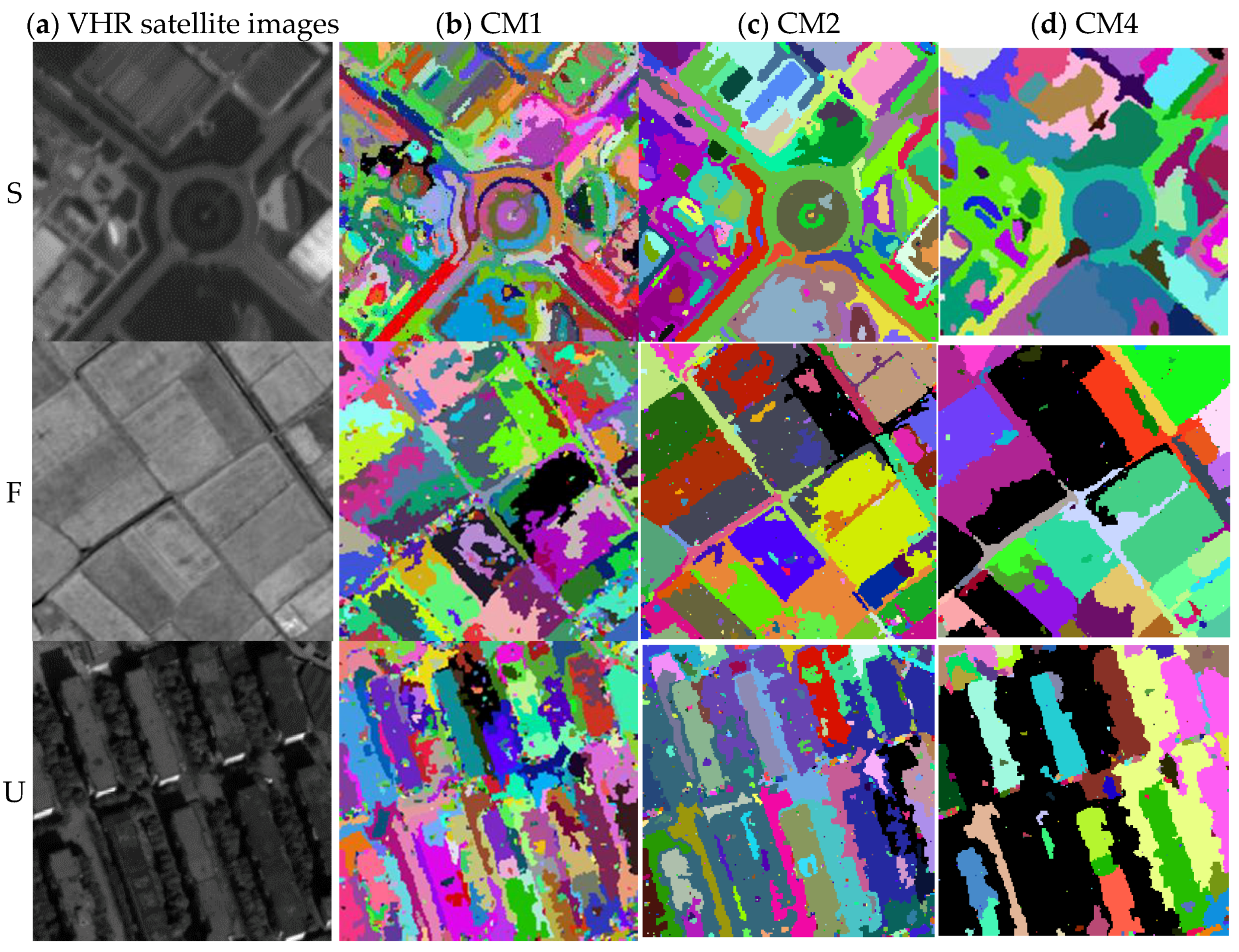
Figure 4 shows the results of over-segmentation over three kinds of geographic scenes, i.e., Suburban (S), Farmland (F), and Urban (U) areas, using the three type of connection modes. The suburban area contains sparse buildings, roads, and fields. The area of farmland consists of cultivated lands with similar shapes and slightly different spectra. In contrast, the urban area displays a large spectral variation, contains many buildings and roads, and has a complex structure. The images come from panchromatic TIANHUI satellites, which have a size of 200 × 200 pixels and a resolution of approximately 2 m.
Four metrics are employed to quantitatively evaluate the quality of image over-segmentations, i.e., the boundary recall (BR) [43], the achievable segmentation accuracy (ASA) [44], the under-segmentation error (UE) [45], and the degree of landscape fragmentation (LF) [42]. The BR is to measure how many percentage of real object boundaries have been discovered by an over-segmentation method. Based on the overlap between segments and real object regions, the ASA and UE is the percentage of pixels within or out of object regions, respectively. The last metric is to measure the degree of fragmentation for an over-segmentation result.
It can be seen from Table 2 that the CM1 is the best connection mode in terms of both BR and ASA for all of the three scenes. In contrast, the CM4 is the best one in terms of LF for all of the three scenes. The CM2 is in the middle among the three connection modes for all of the experiments with the exception of the UE of urban area. Please note that the metrics of both BR and ASA could increase with the number of segments. This also can reflected by the measurement of LF. The FL under CM1 is the highest among the three connection mode for all of three scenes. It also can be seen from Figure 4 that, under the CM1, there exist many segments of very small size, even many isolated points. In contrast, the size of segments is rather large under the CM4 and there explicitly exist under-segmented results. For example, many long and narrow objects, e.g., roads, are often incorrectly merged into larger regions under the CM4. To make full use of characteristics of different connection modes, both CM1 and CM2 will be utilized in our proposed method in Section 3.
3. Edge Dependent Chinese Restaurant Process
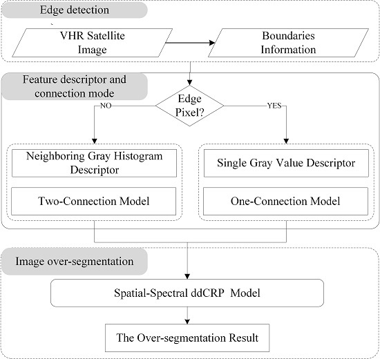
Based on the analysis about the ddCRP in Section 2, we present an improved method for the over-segmentation of VHR satellite images in this section, which is called Edge Dependent Chinese Restaurant Process (EDCRP). As shown in Figure 5, the EDCRP consists of three parts. The first part is edge detection from VHR satellite images. The second part is the selection of the feature descriptor and the connection mode that is based on these detected edges. The third part is image over-segmentation while using the spatial-spectral ddCRP.
3.1. Edge Detection
There exist many methods to extract edge information from images, e.g., the Sobel operator, the Roberts operator, the Prewitt operator, the Laplacian operator, or the Canny operator [46]. All of these methods can be utilized in the proposed method in order to improve the structure integrality of image over-segmentation. In this paper, the Canny operator was adopted since it works better by simultaneously considering both strong and weak edges.
Although the distance between neighboring pixels in the ddCRP could reflect the strength of a potential edge to some degree, there often exist many locations without meaningful edges, while the distance is rather large. Therefore, the detected edges could provide important prior knowledge of image structures for the ddCRP to work better. Given a pixel on an edge, the one-connection mode could provide an opportunity to motivate the model to choose a neighboring pixel with the shortest distance between them in the highest probability (under the assumption that the likelihood is the same value). Consequently, multiple over-segments would occur nearby the pixel in a higher probability. Meanwhile, if the one-connection mode is used everywhere, there would exist many segments of very small size, even many isolated points, as shown in Figure 4. Therefore, the two-connection mode coupled with a gray histogram descriptor is designed to remove these tiny over-segments, in particular isolated points.
3.2. Feature Descriptor and Connection Mode
As for each pixel, there exist two options for feature descriptors and connection modes, which is dependent on whether the pixel is on an edge or not. As for a pixel on an edge, its DN value is used as a feature descriptor and one-connection mode is used to decide which pixels could be tied together. A gray histogram based on neighboring pixels is used to describe a pixel, which is not on any edge and the two-connection mode is used. As shown in Figure 3, the gray histogram descriptor of 6-th pixel in Figure 3 will be constructed by the nine values of 1-th, 2-th, 3-th, 5-th, 6-th, 7-th, 9-th, 10-th, and 11-th pixels. The neighboring gray histogram descriptor is to remove the isolated points in the over-segmentation results. As discussed in the Section 2.3, the merging probability would be approximated to the scaling parameter , when a segment has only a small number of pixels. As shown in Figure 2a–d, the merging probability would be lower than 0.1 and become stable when the number of pixels is larger than about 8. This observation motivate us to use nine pixels instead of individual pixel as a descriptor in the proposed model.
3.3. Spatial-Spectral ddCRP
As discussed in [42], the distance that was constructed with spatial and spectral features is better than only spatial distance. Therefore, both spatial and spectral distances are used in the proposed method. For the sake of clarity, it is called spatial-spectral ddCRP.
4. Experimental Results
In this section, we first described the experimental data. Then, we analyzed the effect of both feature descriptor and connection mode on image over-segmentations. Furthermore, the EDCRP is compared with state of the art methods in terms of quantitative evaluation matrices. At last, we discussed the efficiency and the possible extension of the EDCRP.
4.1. Experimental Data
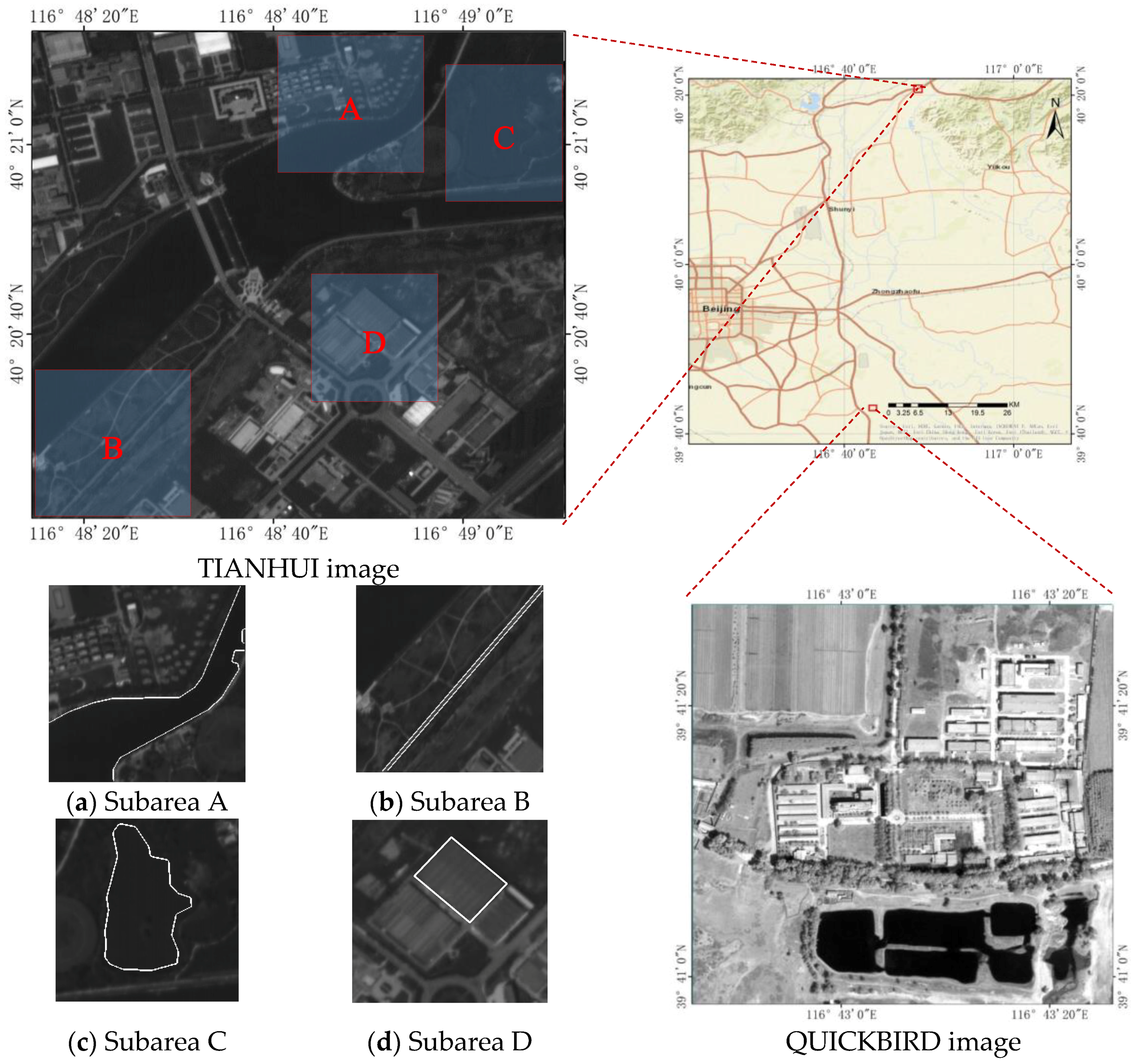
As shown in Figure 6, two panchromatic images from different sensors are used in our experiments. The top-left image is a panchromatic TIANHUI image, which is in Mi Yun district of Beijing, China. The imaging time is 25 July 2013, the resolution is about 2 m, and the size of the image is 800 × 800 pixels. As shown in Figure 6a–d, four subareas of the TIANHUI image, coupled with real boundaries of interested geo-objects, will be employed to illustrate the qualitative effect of both the feature descriptor and the connection mode on over-segmentations in Section 4.2. The bottom-right image in Figure 6 is a panchromatic QUICKBIRD image, which was acquired on 22 April 2006. The area is located in Tong Zhou district of Beijing, China. The size of the image is 900 × 900 pixels with a resolution of 0.60 m.
4.2. Effect of Feature Descriptor and Connection Mode over Over-Segmentations
As shown in Figure 5, the EDCRP can be regard as a mixture of two kinds of feature descriptors and connection modes based on the spatial-spectral ddCRP model. In order to validate the necessary of this kinds of mixture, we compared the results of EDCRP with that of the spatial-spectral ddCRP model under two kinds of combination of both feature descriptor and connection-mode. Specifically, the first combination is that the DN value of each pixel is used as its feature and the one-connection is used. The second combination is that the feature descriptor of each pixel is the gray histogram of its neighboring pixels and the two-connection mode is used. For the sake of simplifying the notation, the two combinations are denoted by ddCRP_1 and ddCRP_2, respectively.
Only the TIANHUI image is used for the analysis in this section. Specifically, we first analyzed the over-segmentations of the two kinds of different combinations from the viewpoint of qualitatively visual inspection. Furthermore, we compared them with that of the proposed method. At last, four quantitative metrics are employed to measure the quality of these over-segmentations.
4.2.1. ddCRP_1
Figure 7 shows the boundaries of over-segments by using the ddCRP_1. Generally speaking, there exist many tiny segments, even isolated points. As shown in the two subfigures, individual geo-objects, e.g., water and building, are over-segmented into many segments. In addition, most of the over-segments wriggle their way along the real boundaries of geo-objects. The structure of over-segments is not very good. For example, there exist two edges along the top-right boundary of the building in subarea D of Figure 7.
4.2.2. ddCRP_2
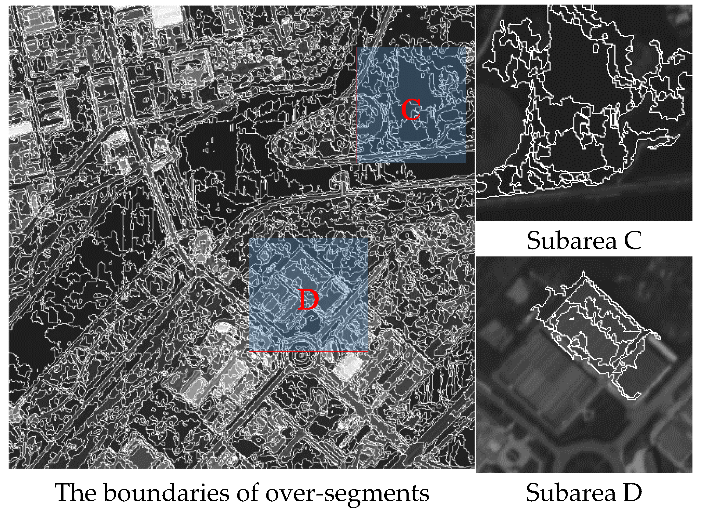
Figure 8 shows the boundaries of over-segmentation using the ddCRP_2. It can be seen that the ddCRP_2 significantly outperforms over the ddCRP_1 in term of structure of over-segment’s boudary. On the one hand, from the viewpoint of overall visual inspection, boudaries of over-segments shown in Figure 8a–d correspond well to boudaries of real geo-objects. For example, as shown in Figure 8c,d, respectively, the boundaries of both water and building look very similar to the real one in terms of the shape of geo-ojects. On the other hand, over-segments of the ddCRP_2 have been pushed into two different directions relative to that of the ddCRP_1. As for the homogeneous regons, over-segments become bigger. Heterogeneous regions have been partioned into more segments of ralative small size. These two kinds of situation can be simultaneously seen in Figure 8d. The top-right part of the building have been merged into a rather large segment, and its bottom-left part have been segmented into multiple small segments with regular boundaries.
In terms of the weakness of the ddCRP_2, on the one hand, there exist too much tiny segments over heterogeneous regions. On the other hand, some different geo-objects have been merged into a large segment. For example, it can be seen from Figure 8a that both the water and part of the land have been merged into a segment. In Figure 8b, the road also be merged with the vegetation along the road into a segment. These objects in Figure 6a,b are expected to be separated by over-segmentation algorithms. However, the ddCRP_2 did not achieve the expected result.
4.2.3. EDCRP
The result of EDCRP is shown in Figure 9. The result of EDCRP is similar with that of the ddCRP_2 in terms of the “shape” of over-segments. We argue that it is reasonable, since the EDCRP can be regarded as a mixture of both the ddCRP_1 and ddCRP_2, which are choosen dependent on pixels on edges or not. Generally speaking, the number of pixels on edges is explicitly less than that of pixels out of edges. Therefore, the EDCRP inherits the strongth of the ddCRP_2, i.e., well struture of over-segments’ boudaries. Fortunately, the EDCRP also rules out the weakness of the ddCRP by using the ddCRP_1 over pixels on detected edges. In other words, the EDCRP would keep two regions being seperated where the ponits have been identified as a point on edges. For example, two different geo-objects in Figure 9a,b have been well seperated into different segments. It is very different from that in Figure 8a,b, which have been merged into large segments.
4.2.4. Quantitive Evaluation
Four metrics are adopted to quantitatively evaluate the quality of over-segmentations, i.e., BR, ASA, UE, and LF. As shown in Table 3, the EDCRP obtains the highest rate of boundary recall (i.e., BR) and achievable segmentation accuracy (ASA). Meanwhile, the EDCRP achieve the lowest error of under-segmentation (UE). As for landscape fragmentation (LF), the ddCRP_2 is the lowest one, with exception of the category building. This result can be explained by the observation in Figure 8 that there exist a large number of tiny segments. For a given image, both BR and ASA would often increase with the number of over-segments. In other words, both BR and ASA would increase with the decrease of LF for a given image. However, both BR and ASA of the EDCRP is the highest one, even when its LF is high than that of the ddCRP_2. In a word, the EDCRP outperforms both ddCRP_1 and ddCRP_2 in terms of all of the four quantitative metrics.
4.3. Comparative Experiments
In this subsection, the EDCRP is compared with three state-of-the-art methods, i.e., Turbo Pixels [47], SLIC [22], and ERS [23] while using the two panchromatic images with different resolutions. These methods are compared from the two viewpoints of both direct and indirect performance evaluation [48,49]. On the one hand, four metrics are utilized to directly evaluate the quality of over-segmentations, i.e., BR, ASA, UE, and LF. On the other hand, the quality of over-segmentations is indirectly evaluated in terms of image classification accuracy.
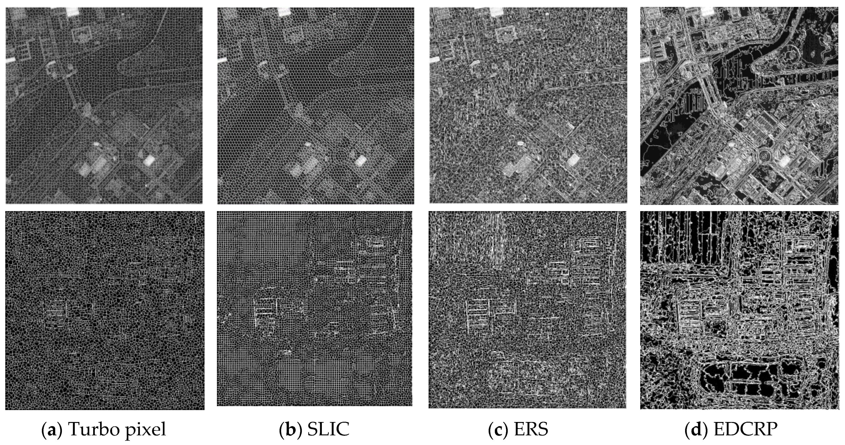
Both the SLIC and ERS achieve image over-segmentation by clustering. Turbo Pixels [47] uses a geometric-flow-based algorithm for acquiring an over-segmentation of an image. For the sake of fairly comparing, the number of clusters for other methods is assigned by the number of all over-segments inferred by the EDCRP. As shown in Figure 10, both SLIC and Turbo pixel generated over-segments with similar size and a more or less convex shape. Their boundaries do not exhibit image structure information. Over-segments produced by ERS have some structure information, but the result has higher complexity in flat area, especially in the water area.
4.3.1. Metrics Based Direct Evaluation
Table 4 lists the values of four metrics of the three approaches for over-segmentation of the TIANHUI image. The ERS achieved the highest rate of boundary recall (i.e., BR) and achievable segmentation accuracy (ASA) among the three methods for all of four kinds of geo-object categories. As for the under-segmentation error (UE), the ERS is the lowest with the exception of the category water. The ERS also obtained a relative low value of LF. Based on these quantitative evaluation, the ERS outperform both the Turbo pixel and SLIC.
However, when compared with the EDCRP, the ERS achieved a lower value of both BR and ASA, and a rather higher value of both UE and LF. In other words, the EDCRP outperform all of the sate-of-the-art methods for over-segmentation in terms of four quantitative metrics. As for visual inspection, the over-segmentation result that is produced by ERS is similar with that of the EDCRP in terms of structure of over-segments. The significant difference is that ERS still produces rather small segments, even for homogeneous regions, e.g., water.
Table 5 lists the values of four metrics of the four approaches to the over-segmentation of the QUICKBIRD image. The EDCRP exhibits the best performance in terms of three metrics, i.e., BR, UE and LF. As for the achievable segmentation accuracy, EDCRP is only lower than the ERS, and higher than both Turbo pixel and SLIC.
4.3.2. Classification Based Indirect Evaluation
Image over-segments are often used as objects for classification. In our experiments, random forests with 100 trees are trained as classifiers using randomly selected 50% over-segments. Table 6 lists both the Overall Accuracy (OA) and kappa of the classifier. The EDCRP outperforms other three approaches for image over-segmentation in terms of classification accuracy.
Figure 11 shows the classification maps of the TIANHUI image. It can be seen from the classification maps that there exists rather explicit fingerprints of the over-segments. For example, the building in the subarea D, there exist misclassified blobs with convex shape in the subfigure (d) and (e) of Figure 11. In the subarea C, there exists explicit wriggled boundary of water in the subfigure (f) of Figure 11. In contrast, the classification map of EDCRP exhibits very good structure integrality for almost geo-objects. Specifically, as shown in the subarea B of Figure 11c, the wriggled path has been well classified.
4.4. Discussions
In this section, we disscuss the efficiency and possible extensions of the EDCRP.
4.4.1. Efficiency
Since the number of clusters is also a random variable to be inferred in a nonparametric Bayesian clustering model, the process of clustering need more time than the parametric clustering method to be a convergence state. As shown in Equation (4), the posterior of customer assignments are approximated by using Gibbs sampling. A reliable sample would be generated only when the process of sampling reach a stable state. It can be seen from Table 7 that the efficiency of the proposed method is explicitly lower than that of the state of the art methods for image over-segmentation. Therefore, it deserves investigation as to how to significantly enhance the efficiency of the EDCRP in the future.
4.4.2. Possible Extensions
Although the present model has only been applied to the VHR panchromatic image in this paper, it is straightforward to extend the EDCRP to the over-segmentation of multi-spectral images [50,51,52]. It can be seen from Equation (4) that the posterior of customer assignments can be approximated if both the likelihood and distance dependent terms can be well defined. Given a multispectral image, the likelihood in Equation (5) can be defined by replacing the multinomial distribution for discrete DN values with Gaussian distribution for multi-spectral satellite images.
5. Conclusions
In this paper, we systematically analyzed the characteristics of components in the ddCRP for VHR panchromatic image over-segmentation, i.e., distance dependent term, likelihood term, and connection mode among neighboring pixels. Furthermore, we present an improved nonparametric Bayesian method, which is called Edge Dependent Chinese Restaurant Process (EDCRP). Experimental results show that the presented methods outperform the state of the art over-segmentation methods in terms of both four evaluation metrics, i.e., under-segmentation error (UE), the boundary recall (BR), the achievable segmentation accuracy (ASA), and the degree of landscape fragmentation (LF) and classification accuracies. In the future, we would investigate how to speed the process of inferring customer assignments, and extend the present method to over-segment VHR multi-spectral satellite images.
Author Contributions
Conceptualization, H.T.; Funding acquisition, H.T.; Investigation, H.T. and X.-J.Z.; Methodology, X.-J.Z.; Software, X.-J.Z. and W.H.; Supervision, H.T.
Acknowledgments
This work was supported by the National Key R&D Program of China (No. 2017YFB0504104) and the National Natural Science Foundation of China (No. 41571334).
Conflicts of Interest
The authors declare no conflicts of interest.
References
- Benediktsson, J.A.; Chanussot, J.; Moon, W.M. Very high-resolution remote sensing: Challenges and opportunities [point of view]. Proc. IEEE 2012, 100, 1907–1910. [Google Scholar] [CrossRef]
- Bjorgo, E. Very high resolution satellites: A new source of information in humanitarian relief operations. Bull. Assoc. Inf. Sci. Technol. 1999, 26, 22–24. [Google Scholar] [CrossRef]
- Marchisio, G.; Pacifici, F.; Padwick, C. On the relative predictive value of the new spectral bands in the WorldWiew-2 sensor. In Proceedings of the 2010 IEEE International Geoscience and Remote Sensing Symposium, Honolulu, HI, USA, 25–30 July 2010; pp. 2723–2726. [Google Scholar] [CrossRef]
- Saito, K.; Spence, R.J.; Going, C.; Markus, M. Using high-resolution satellite images for post-earthquake building damage assessment: A study following the 26 January 2001 gujarat earthquake. Earthq. Spectra 2004, 20, 145–169. [Google Scholar] [CrossRef]
- Tralli, D.M.; Blom, R.G.; Zlotnicki, V.; Donnellan, A.; Evans, D.L. Satellite remote sensing of earthquake, volcano, flood, landslide and coastal inundation hazards. ISPRS J. Photogramm. Remote Sens. 2005, 59, 185–198. [Google Scholar] [CrossRef]
- Shalaby, A.; Tateishi, R. Remote sensing and gis for mapping and monitoring land cover and land-use changes in the northwestern coastal zone of egypt. Appl. Geogr. 2007, 27, 28–41. [Google Scholar] [CrossRef]
- Zhou, W.; Huang, G.; Troy, A.; Cadenasso, M. Object-based land cover classification of shaded areas in high spatial resolution imagery of urban areas: A comparison study. Remote Sens. Environ. 2009, 113, 1769–1777. [Google Scholar] [CrossRef]
- Atzberger, C. Advances in remote sensing of agriculture: Context description, existing operational monitoring systems and major information needs. Remote Sens. 2013, 5, 949–981. [Google Scholar] [CrossRef]
- Brown, J.C.; Jepson, W.E.; Kastens, J.H.; Wardlow, B.D.; Lomas, J.M.; Price, K. Multitemporal, moderate-spatial-resolution remote sensing of modern agricultural production and land modification in the brazilian amazon. GISci. Remote Sens. 2007, 44, 117–148. [Google Scholar] [CrossRef]
- Reinartz, P.; Müller, R.; Lehner, M.; Schroeder, M. Accuracy analysis for DSM and orthoimages derived from spot hrs stereo data using direct georeferencing. ISPRS J. Photogramm. Remote Sens. 2006, 60, 160–169. [Google Scholar] [CrossRef]
- Holland, D.; Boyd, D.; Marshall, P. Updating topographic mapping in great britain using imagery from high-resolution satellite sensors. ISPRS J. Photogramm. Remote Sens. 2006, 60, 212–223. [Google Scholar] [CrossRef]
- Tighe, J.; Lazebnik, S. Superparsing: Scalable nonparametric image parsing with superpixels. In Proceedings of the European Conference on Computer Vision, Crete, Greece, 5–11 September 2010; Springer: Berlin, Germany, 2010; pp. 352–365. [Google Scholar]
- Haralick, R.M.; Shapiro, L.G. Image segmentation techniques. Comput. Vis. Graph. Image Process. 1985, 29, 100–132. [Google Scholar] [CrossRef]
- Schalkoff, R.J. Digital Image Processing and Computer Vision; Wiley: New York, NY, USA, 1989; Volume 286. [Google Scholar]
- Forsyth, D.A.; Ponce, J. Computer Vision: A Modern Approach; Prentice Hall Professional Technical Reference: Upper Saddle River, NJ, USA, 2002. [Google Scholar]
- Van de Sande, K.E.; Uijlings, J.R.; Gevers, T.; Smeulders, A.W. Segmentation as selective search for object recognition. In Proceedings of the 2011 IEEE International Conference on Computer Vision (ICCV), Barcelona, Spain, 6–11 November 2011; IEEE: New York, NY, USA, 2011; pp. 1879–1886. [Google Scholar]
- Belongie, S.; Malik, J.; Puzicha, J. Shape matching and object recognition using shape contexts. IEEE Trans. Pattern Anal. Mach. Intell. 2002, 24, 509–522. [Google Scholar] [CrossRef] [Green Version]
- Belongie, S.; Carson, C.; Greenspan, H.; Malik, J. Color-and texture-based image segmentation using em and its application to content-based image retrieval. In Proceedings of the 1998 Sixth International Conference on Computer Vision, Bombay, India, 4–7 January 1998; IEEE: New York, NY, USA, 1998; pp. 675–682. [Google Scholar]
- Sural, S.; Qian, G.; Pramanik, S. Segmentation and histogram generation using the HSV color space for image retrieval. In Proceedings of the 2002 International Conference on Image Processing, Rochester, NY, USA, 22–25 September 2002; IEEE: New York, NY, USA, 2002; p. II. [Google Scholar]
- Carson, C.; Belongie, S.; Greenspan, H.; Malik, J. Blobworld: Image segmentation using expectation-maximization and its application to image querying. IEEE Trans. Pattern Anal. Mach. Intell. 2002, 24, 1026–1038. [Google Scholar] [CrossRef]
- Harchaoui, Z.; Bach, F. Image classification with segmentation graph kernels. In Proceedings of the IEEE Conference on Computer Vision and Pattern Recognition (CVPR’07), Boston, MA, USA, 7–12 June 2007; IEEE: New York, NY, USA, 2007; pp. 1–8. [Google Scholar]
- Achanta, R.; Shaji, A.; Smith, K.; Lucchi, A.; Fua, P.; Süsstrunk, S. Slic superpixels compared to state-of-the-art superpixel methods. IEEE Trans. Pattern Anal. Mach. Intell. 2012, 34, 2274–2282. [Google Scholar] [CrossRef] [PubMed]
- Liu, M.-Y.; Tuzel, O.; Ramalingam, S.; Chellappa, R. Entropy rate superpixel segmentation. In Proceedings of the 2011 IEEE Conference on Computer Vision and Pattern Recognition (CVPR), Colorado Springs, CO, USA, 20–25 June 2011; IEEE: New York, NY, USA, 2011; pp. 2097–2104. [Google Scholar]
- Shi, J.; Malik, J. Normalized cuts and image segmentation. IEEE Trans. Pattern Anal. Mach. Intell. 2000, 22, 888–905. [Google Scholar] [Green Version]
- Comaniciu, D.; Meer, P. Mean shift analysis and applications. In Proceedings of the Seventh IEEE International Conference on Computer Vision, Kerkyra, Greece, 20–27 September 1999; IEEE: New York, NY, USA, 1999; pp. 1197–1203. [Google Scholar] [Green Version]
- Yuan, J.; Gleason, S.S.; Cheriyadat, A.M. Systematic benchmarking of aerial image segmentation. IEEE Geosci. Remote Sens. Lett. 2013, 10, 1527–1531. [Google Scholar] [CrossRef]
- Yuan, J.; Wang, D.; Cheriyadat, A.M. Factorization-based texture segmentation. IEEE Trans. Image Process. 2015, 24, 3488–3497. [Google Scholar] [CrossRef] [PubMed]
- Davis, L.S.; Rosenfeld, A.; Weszka, J.S. Region extraction by averaging and thresholding. IEEE Trans. Syst. Man Cybern. 1975, 5, 383–388. [Google Scholar] [CrossRef]
- Kohler, R. A segmentation system based on thresholding. Comput. Graph. Image Process. 1981, 15, 319–338. [Google Scholar] [CrossRef]
- Zadeh, L.A. Some reflections on soft computing, granular computing and their roles in the conception, design and utilization of information/intelligent systems. Soft Comput. 1998, 2, 23–25. [Google Scholar] [CrossRef]
- Senthilkumaran, N.; Rajesh, R. A study on edge detection methods for image segmentation. In Proceedings of the International Conference on Mathematics and Computer Science (ICMCS-2009), Chennai, India, 5–6 January 2009; pp. 255–259. [Google Scholar]
- Sinop, A.K.; Grady, L. A seeded image segmentation framework unifying graph cuts and random walker which yields a new algorithm. In Proceedings of the 2007 IEEE 11th International Conference on Computer Vision (ICCV 2007), Rio de Janeiro, Brazil, 14–21 October 2007; IEEE: New York, NY, USA, 2007; pp. 1–8. [Google Scholar]
- Grady, L. Multilabel random walker image segmentation using prior models. In Proceedings of the IEEE Computer Society Conference on Computer Vision and Pattern Recognition (CVPR 2005), San Diego, CA, USA, 20–25 June 2005; IEEE: New York, NY, USA, 2005; pp. 763–770. [Google Scholar]
- Comaniciu, D.; Meer, P. Mean shift: A robust approach toward feature space analysis. IEEE Trans. Pattern Anal. Mach. Intell. 2002, 24, 603–619. [Google Scholar] [CrossRef]
- Purohit, P.; Joshi, R. A new efficient approach towards k-means clustering algorithm. Int. J. Comput. Sci. Commun. Netw. 2013, 4, 125–129. [Google Scholar]
- Sammut, C.; Webb, G.I. Encyclopedia of Machine Learning; Springer Science & Business Media: Berlin, Germany, 2011. [Google Scholar]
- Blei, D.M.; Frazier, P.I. Distance dependent chinese restaurant processes. J. Mach. Learn. Res. 2011, 12, 2461–2488. [Google Scholar]
- Mao, T.; Tang, H.; Wu, J.; Jiang, W.; He, S.; Shu, Y. A Generalized Metaphor of Chinese Restaurant Franchise to Fusing Both Panchromatic and Multispectral Images for Unsupervised Classification. IEEE Trans. Geosci. Remote Sens. 2016, 54, 4594–4604. [Google Scholar] [CrossRef]
- Li, S.; Tang, H.; He, S.; Shu, Y.; Mao, T.; Li, J.; Xu, Z. Unsupervised Detection of Earthquake-Triggered Roof-Holes From UAV Images Using Joint Color and Shape Features. IEEE Geosci. Remote Sens. Lett. 2015, 12, 1823–1827. [Google Scholar]
- Shu, Y.; Tang, H.; Li, J.; Mao, T.; He, S.; Gong, A.; Chen, Y.; Du, H. Object-Based Unsupervised Classification of VHR Panchromatic Satellite Images by Combining the HDP and IBP on Multiple Scenes. IEEE Trans. Geosci. Remote Sens. 2015, 53, 6148–6162. [Google Scholar] [CrossRef]
- Yi, W.; Tang, H.; Chen, Y. An Object-Oriented Semantic Clustering Algorithm for High-Resolution Remote Sensing Images Using the Aspect Model. IEEE Geosci. Remote Sens. Lett. 2011, 8, 522–526. [Google Scholar] [CrossRef]
- Zhai, X.; Niu, X.; Tang, H.; Mao, T. Distance dependent chinese restaurant process for VHR satellite image oversegmentation. In Proceedings of the 2017 Joint Urban Remote Sensing Event (JURSE), Dubai, United Arab Emirates, 6–8 March 2017; IEEE: New York, NY, USA, 2017; pp. 1–4. [Google Scholar]
- Ren, X.; Malik, J. Learning a Classification Model for Segmentation. In Null; IEEE: New York, NY, USA, 2003; p. 10. [Google Scholar]
- Nowozin, S.; Gehler, P.V.; Lampert, C.H. On parameter learning in CRF-based approaches to object class image segmentation. In Proceedings of the European Conference on Computer Vision, Crete, Greece, 5–11 September 2010; Springer: Berlin, Germany, 2010; pp. 98–111. [Google Scholar]
- Veksler, O.; Boykov, Y.; Mehrani, P. Superpixels and supervoxels in an energy optimization framework. In Proceedings of the European Conference on Computer Vision, Crete, Greece, 5–11 September 2010; Springer: Berlin, Germany, 2010; pp. 211–224. [Google Scholar]
- Jain, R.; Kasturi, R.; Schunck, B.G. Machine Vision; McGraw-Hill: New York, NY, USA, 1995; Volume 5. [Google Scholar]
- Levinshtein, A.; Stere, A.; Kutulakos, K.N.; Fleet, D.J.; Dickinson, S.J.; Siddiqi, K. Turbopixels: Fast superpixels using geometric flows. IEEE Trans. Pattern Anal. Mach. Intell. 2009, 31, 2290–2297. [Google Scholar] [CrossRef] [PubMed]
- Stutz, D.; Alexander, H.; Bastian, L. Superpixels: An evaluation of the state-of-the-art. Comput. Vis. Image Underst. 2018, 166, 1–27. [Google Scholar] [CrossRef] [Green Version]
- Giraud, R.; Ta, V.T.; Papadakis, N. Robust superpixels using color and contour features along linear path. Comput. Vis. Image Underst. 2018, 170, 1–13. [Google Scholar] [CrossRef] [Green Version]
- Benedek, C.; Descombes, X.; Zerubia, J. Building development monitoring in multitemporal remotely sensed image pairs with stochastic birth-death dynamics. IEEE Trans. Pattern Anal. Mach. Intell. 2012, 34, 33–50. [Google Scholar] [CrossRef] [PubMed] [Green Version]
- Grinias, I.; Panagiotakis, C.; Tziritas, G. MRF-based Segmentation and Unsupervised Classification for Building and Road Detection in Peri-urban Areas of High-resolution. ISPRS J. Photogramm. Remote Sens. 2016, 122, 45–166. [Google Scholar] [CrossRef]
- The, J.W.; Jordan, M.I.; Beal, M.J. Hierarchical Dirichlet processes. J. Am. Stat. Assoc. 2006, 101, 1566–1581. [Google Scholar]
Figure 1.
The illustration of distance dependent Chinese restaurant process (ddCRP) for image over-segmentation; (a) an image (i.e., a restaurant) with 16 pixels (i.e., customers) where each numbered square denotes a pixel; (b) each arrow indicates a customer choose to sit with another customer; and, (c) a segment consists of pixels with a same color and every two pixels within a segment can reach to each other along the inferred customer assignments.

Figure 2.
Five experiments are shown in subfigures (a–e), respectively. As for each experiment, the left subfigure shows a paired of Gaussian distributions, which are utilized to generate DN values of two over-segments, respectively; the right one is the distribution of the merging probability over the numbers of pixels within the two over-segments.


Figure 3.
Three kinds of connection modes, (a) the one-connection mode (CM1), (b) the two-connection mode (CM2), and (c) the four-connection mode (CM4).
Figure 3.
Three kinds of connection modes, (a) the one-connection mode (CM1), (b) the two-connection mode (CM2), and (c) the four-connection mode (CM4).

Figure 4.
Over-segmentation of Very High Resolution (VHR) satellite images using the ddCRP with different connection modes: (a) VHR satellite images of three kinds of scenes, i.e., Suburb (S), Farmland (F), and Urban (U) areas, and corresponding over-segmentations using the ddCRP with (b) one-connection mode (CM1), (c) the two-connection mode (CM2), and (d) the four-connection mode (CM4), respectively.

Figure 5.
The flowchart of Edge Dependent Chinese Restaurant Process (EDCRP) for image over-segmentation.
Figure 5.
The flowchart of Edge Dependent Chinese Restaurant Process (EDCRP) for image over-segmentation.

Figure 6.
Two VHR satellite images used in our experiments, where subfigures (a–d) show the subarea A, B, C, and D coupled with boundaries of interested geo-objects, respectively.
Figure 6.
Two VHR satellite images used in our experiments, where subfigures (a–d) show the subarea A, B, C, and D coupled with boundaries of interested geo-objects, respectively.

Figure 7.
The boundaries of over-segments obtained by using the ddCRP_1 from the TIANHUI image. Both subareas C and D coupled with over-segments are shown in the two right-side subfigures.
Figure 7.
The boundaries of over-segments obtained by using the ddCRP_1 from the TIANHUI image. Both subareas C and D coupled with over-segments are shown in the two right-side subfigures.

Figure 8.
The boundaries of over-segments obtained by using the ddCRP_2 from the experimental image. The subfigures (a–d) are zoomed results from subareas A, B, C, and D, respectively.
Figure 8.
The boundaries of over-segments obtained by using the ddCRP_2 from the experimental image. The subfigures (a–d) are zoomed results from subareas A, B, C, and D, respectively.

Figure 9.
The boundaries of over-segments obtained by using the EDCRP from the experimental image. The subfigures (a–d) are zoomed results from subareas A, B, C, and D, respectively.
Figure 9.
The boundaries of over-segments obtained by using the EDCRP from the experimental image. The subfigures (a–d) are zoomed results from subareas A, B, C, and D, respectively.

Figure 10.
The over-segmentation results over both TIANHUI (first row) and QUICKBIRD (second row) images using four over-segmentation methods, i.e., (a) Turbo pixel, (b) Simple Linear Iterative Clustering (SLIC), (c) Entropy Rate Superpixel segmentation (ERS), and (d) Edge Dependent Chinese Restaurant Process (EDCRP).

Figure 11.
Classification maps of the TIANHUI image based on the over-segments; (a) is the TIANHUI image; (b) is the ground-truth of the image; (c–f) are the classification maps based on the over-segments produced by the EDCRP, Turbo Pixel, SLIC, and ERS, respectively. The legend shows the class labels in both the ground-truth and classification maps.


Table 1.
Parameters of paired Gaussian distributions used in the five experiments.
| (a) | (b) | (c) | (d) | (e) | |
|---|---|---|---|---|---|
| kth over-segment | = 45, = 0.1 | = 45, = 2 | = 50, = 2 | = 55, = 2 | = 58, = 2 |
| lth over-segment | = 60, = 0.1 | = 60, = 2 | = 60, = 2 | = 60, = 2 | = 60, = 2 |
Table 2.
The quantitative evaluation of over-segmentations using the ddCRP over three type of geo-scenes, i.e., Suburban (S), Farmland (F), and Urban (U) areas, under three kinds of connection modes, i.e., one-connection mode (CM1), two-connection mode (CM2), and four-connection mode (CM4), respectively. For every evaluation metric, the best performance among different connection modes was marked as red or blue bold.
| Suburban | Farmland | Urban | |||||||
|---|---|---|---|---|---|---|---|---|---|
| CM1 | CM2 | CM4 | CM1 | CM2 | CM4 | CM1 | CM2 | CM4 | |
| BR | 0.8 | 0.67 | 0.5 | 0.79 | 0.70 | 0.57 | 0.81 | 0.66 | 0.51 |
| ASA | 0.84 | 0.67 | 0.64 | 0.87 | 0.6 | 0.55 | 0.89 | 0.59 | 0.59 |
| UE | 0.07 | 0.09 | 0.15 | 0.11 | 0.12 | 0.15 | 0.09 | 0.07 | 0.09 |
| LF | 0.85 | 0.54 | 0.42 | 0.92 | 0.73 | 0.41 | 0.42 | 0.68 | 0.48 |
Table 3.
The quantitative evaluation of over-segmentation.
| Building | Water | Bare Land | Road | |||||||||
|---|---|---|---|---|---|---|---|---|---|---|---|---|
| ddCRP_1 | ddCRP_2 | EDCRP | ddCRP_1 | ddCRP_2 | EDCRP | ddCRP_1 | ddCRP_2 | EDCRP | ddCRP_1 | ddCRP_2 | EDCRP | |
| BR | 0.891 | 0.8946 | 0.9027 | 0.857 | 0.8436 | 0.8839 | 0.8405 | 0.8424 | 0.8918 | 0.9029 | 0.9030 | 0.9461 |
| ASA | 0.3834 | 0.4957 | 0.5023 | 0.1979 | 0.2013 | 0.2154 | 0.2057 | 0.3473 | 0.3619 | 0.2481 | 0.279 | 0.3619 |
| UE | 0.4698 | 0.4523 | 0.4016 | 0.3019 | 0.3024 | 0.2714 | 0.5467 | 0.5647 | 0.5183 | 0.4688 | 0.4636 | 0.4258 |
| LF | 0.0304 | 0.0214 | 0.0204 | 0.0595 | 0.0387 | 0.033 | 0.8405 | 0.0258 | 0.8918 | 0.0286 | 0.0231 | 0.0254 |
Table 4.
The evaluation of over-segmentations of TIANHUI image while using Turbo Pixel (TP), SLIC and ERS.
Table 4.
The evaluation of over-segmentations of TIANHUI image while using Turbo Pixel (TP), SLIC and ERS.
| Building | Water | Bare Land | Road | |||||||||
|---|---|---|---|---|---|---|---|---|---|---|---|---|
| TP | SLIC | ERS | TP | SLIC | ERS | TP | SLIC | ERS | TP | SLIC | ERS | |
| BR | 0.6675 | 0.6563 | 0.8723 | 0.625 | 0.6461 | 0.8327 | 0.6461 | 0.6229 | 0.8369 | 0.719 | 0.6847 | 0.8884 |
| ASA | 0.188 | 0.1766 | 0.2039 | 0.0112 | 0.0095 | 0.0141 | 0.0782 | 0.0715 | 0.0899 | 0.0956 | 0.0877 | 0.1009 |
| UE | 0.662 | 0.689 | 0.478 | 0.3247 | 0.3001 | 0.3197 | 0.6844 | 0.701 | 0.5772 | 0.5983 | 0.6226 | 0.4639 |
| LF | 0.0448 | 0.0372 | 0.0403 | 0.0672 | 0.0671 | 0.0648 | 0.0426 | 0.0385 | 0.0419 | 0.0482 | 0.0395 | 0.033 |
Table 5.
The quantitative evaluation of different over-segmentations of QUICKBIRD image.
| Metric | Turbo Pixel | SLIC | ERS | EDCRP |
|---|---|---|---|---|
| BR | 0.6953 | 0.7979 | 0.7675 | 0.8452 |
| ASA | 0.8912 | 0.8810 | 0.9191 | 0.8978 |
| UE | 0.0799 | 0.0679 | 0.0592 | 0.0542 |
| LF | 0.013 | 0.015 | 0.014 | 0.008 |
Table 6.
The Overall Accuracy (OA) and kappa of the classifier over both the TIANHUI and QUICKBIRD images.
Table 6.
The Overall Accuracy (OA) and kappa of the classifier over both the TIANHUI and QUICKBIRD images.
| Image | Metric | Turbo Pixel | SLIC | ERS | EDCRP |
|---|---|---|---|---|---|
| TIANHUI | OA | 0.7551 | 0.7706 | 0.7796 | 0.7878 |
| Kappa | 0.6751 | 0.7012 | 0.7056 | 0.7152 | |
| QUICKBIRD | OA | 0.8171 | 0.8116 | 0.7753 | 0.8189 |
| Kappa | 0.7740 | 0.7681 | 0.7251 | 0.7759 |
Table 7.
The running time of different approaches for image over-segmentation.
| Turbo Pixel | SLIC | ERS | EDCRP | |
|---|---|---|---|---|
| Time (s) | 374 | 75 | 416 | 4981 |
© 2018 by the authors. Licensee MDPI, Basel, Switzerland. This article is an open access article distributed under the terms and conditions of the Creative Commons Attribution (CC BY) license (http://creativecommons.org/licenses/by/4.0/).
Share and Cite
MDPI and ACS Style
Tang, H.; Zhai, X.; Huang, W. Edge Dependent Chinese Restaurant Process for Very High Resolution (VHR) Satellite Image Over-Segmentation. Remote Sens. 2018, 10, 1519. https://doi.org/10.3390/rs10101519
AMA Style
Tang H, Zhai X, Huang W. Edge Dependent Chinese Restaurant Process for Very High Resolution (VHR) Satellite Image Over-Segmentation. Remote Sensing. 2018; 10(10):1519. https://doi.org/10.3390/rs10101519
Chicago/Turabian StyleTang, Hong, Xuejun Zhai, and Wei Huang. 2018. "Edge Dependent Chinese Restaurant Process for Very High Resolution (VHR) Satellite Image Over-Segmentation" Remote Sensing 10, no. 10: 1519. https://doi.org/10.3390/rs10101519
Note that from the first issue of 2016, this journal uses article numbers instead of page numbers. See further details here.