Article

Scale Matters: Spatially Partitioned Unsupervised Segmentation Parameter Optimization for Large and Heterogeneous Satellite Images

1
Department of Geosciences, Environment & Society, Université libre de Bruxelles (ULB), 1050 Bruxelles, Belgium
2
Natural Resources and Ecosystem Services Area, Institute for Global Environmental Strategies, 2108-11 Kamiyamaguchi, Hayama, Kanagawa 240-0115, Japan
*
Author to whom correspondence should be addressed.
Remote Sens. 2018, 10(9), 1440; https://doi.org/10.3390/rs10091440
Submission received: 13 August 2018 / Revised: 3 September 2018 / Accepted: 5 September 2018 / Published: 9 September 2018
(This article belongs to the Special Issue Image Segmentation for Environmental Monitoring)

Abstract

:
To classify Very-High-Resolution (VHR) imagery, Geographic Object Based Image Analysis (GEOBIA) is the most popular method used to produce high quality Land-Use/Land-Cover maps. A crucial step in GEOBIA is the appropriate parametrization of the segmentation algorithm prior to the classification. However, little effort has been made to automatically optimize GEOBIA algorithms in an unsupervised and spatially meaningful manner. So far, most Unsupervised Segmentation Parameter Optimization (USPO) techniques, assume spatial stationarity for the whole study area extent. This can be questionable, particularly for applications in geographically large and heterogeneous urban areas. In this study, we employed a novel framework named Spatially Partitioned Unsupervised Segmentation Parameter Optimization (SPUSPO), which optimizes segmentation parameters locally rather than globally, for the Sub-Saharan African city of Ouagadougou, Burkina Faso, using WorldView-3 imagery (607 km2). The results showed that there exists significant spatial variation in the optimal segmentation parameters suggested by USPO across the whole scene, which follows landscape patterns—mainly of the various built-up and vegetation types. The most appropriate automatic spatial partitioning method from the investigated techniques, was an edge-detection cutline algorithm, which achieved higher classification accuracy than a global optimization, better predicted built-up regions, and did not suffer from edge effects. The overall classification accuracy using SPUSPO was 90.5%, whilst the accuracy from undertaking a traditional USPO approach was 89.5%. The differences between them were statistically significant (p < 0.05) based on a McNemar’s test of similarity. Our methods were validated further by employing a segmentation goodness metric, Area Fit Index (AFI)on building objects across Ouagadougou, which suggested that a global USPO was more over-segmented than our local approach. The mean AFI values for SPUSPO and USPO were 0.28 and 0.36, respectively. Finally, the processing was carried out using the open-source software GRASS GIS, due to its efficiency in raster-based applications.

Graphical Abstract

1. Introduction

Accurate and precise Land-Use/Land-Cover (LULC) maps derived from remotely sensed imagery are crucial for applications spanning several fields, including spatial planning, population estimation, environmental monitoring, and socio-economic and epidemiological modelling [1,2,3,4]. These map products not only provide useful information on their own, but also through their use as an input to secondary models (e.g., population distribution models [3], hydrological models [5], or LULC change models [6,7,8]. As such, maximizing the accuracy of LULC maps is a critical methodological facet in reducing error propagation and enhancing the effectiveness of science-based policy-making.
For the classification of high- and very-high resolution (VHR) imagery in particular, Geographic Object-Based Image (GEOBIA) analysis has been established as a superior method over traditional pixel-based approaches [9], as it produces a semantic representation of data closer to reality than the arbitrary nature of pixels [10]. Recent studies have attempted to establish a formal ontological framework to further advance the use of objects as spatial representation units [11]. In GEOBIA, the most crucial step before classification is the clustering of neighboring image pixels into segments based on spatial, spectral, and contextual criteria [12]. These segments should ideally represent real world objects or LC categories (e.g., building rooftops, or agricultural fields) that are larger than the original image resolution [13]. As several studies have demonstrated, GEOBIA classification accuracy is not only affected by the classification algorithm itself [14], but also by the quality of the extracted image segmentation [15,16,17,18]. Consequently, the selection of an appropriate segmentation (i.e., object-creating) algorithm, as well as its parametrization, are crucial with respect to the final output [19,20,21].
Region-growing (RG) segmentation techniques are the most popular in GEOBIA literature, mainly due to their implementation through the multiresolution segmentation algorithm [22], implemented in the popular software eCognition (Definiens) [16,23,24,25,26]. The most important parameter in RG segmentation is the Threshold Parameter (TP; e.g., the Scale Parameter of the multiresolution segmentation algorithm in eCognition), which governs the average size of the created segments. The selection of the parameter is most commonly attempted through a time consuming, user dependent, trial and error process [27,28], in which the quality of the produced segmentations is assessed visually [29], or through a quantitative comparison against reference data (i.e., manually digitized polygons based on visual image interpretation) [30,31,32]. These approaches have been criticized for being untenable due to their subjective nature and time inefficiency, whilst at the same time, the improvement they can offer in classification accuracy might be limited [33]. Therefore, other research has been directed towards the development of objectively defined Unsupervised Segmentation Parameter Optimization (USPO) techniques, which evaluate individual segmentations based on geostatistical metrics and do not require reference data [34,35,36]. To do so, various USPO metrics have been proposed, such as the rate of change in local variance implemented through the estimation of scale parameter tool (ESP) [34,37], the optimization of objective functions such as the Global Score (GS) [38] and the F-measure [18,39] among others, with varying degrees of success. In the comparative study of Grybas et al. [23], the F-measure was found superior to the ESP and GS, potentially due to its sensitivity to over and under segmentation. The GS and F-measure assess spectral values within (i.e., Weighted Variance (WV)) and between (i.e., Global Moran’s I (MI)) segments. Ideally, an accurate segmentation should minimize the spectral heterogeneity within segments and maximize the spectral heterogeneity between segments, so the TP that is found to maximize the aforementioned function is accredited to be optimal [40].
So far, the optimization of segment-creating algorithms (and in this study, the region growing one), has been attempted mainly through the use of global methods, either at single or multiple scales [36,37]. A global approach implies that the optimization of the TP is adequate using the whole extent of the study area or a subset which is assumed to be representative [15,33,41]. The vast majority of the developments in the past years operate on that assumption, a situation exaggerated from the relatively small study areas that are used (<3 km2 in ~95% of the recent literature on object-based land cover mapping) as pointed out in the review of Ma et al. [42]. These approaches assume spatial stationarity—that the relationship between input data and the segment generating process is stable across space which is reflected by having a spatially invariant TP for the whole study area. However, this begs the question “Why is the extent of the study area in a remote sensing application automatically assumed to be the most appropriate scale to optimize the segmentation algorithms?”. This is of increasing importance as it has been recently demonstrated that partitioning the study area in smaller regions can provide significantly different results, highlighting the effect of geographic scale in remote sensing operations [43,44]. Spatial stationarity might hold for small homogenous regions, but perhaps is unsuitable for large and/or heterogenous scenes. It would be sensible to hypothesize that the optimal TP would intrinsically and significantly vary across space due to local variations in data structure, particularly for urban areas, which are known for their landscape variability even within the same LULC class. If a global approach would be used in such a case, it might only capture an average and potentially misleading impression of the situation and lead towards adding bias to the segmentation model, which could be reflected both in segmentation evaluation metrics and classification accuracy. In recent years, few studies have tackled this issue by employing more localized or regionalized procedures.
Johnson and Xie [36] refined their global segmentation results in a two-stage procedure by re-segmenting local outliers using geospatial metrics such as Local Moran’s I. Cánovas-García and Alonso-Sarría [43] demonstrated improvements in segmentation quality by optimizing the TP independently in agricultural plots, instead of selecting a single parameter for the whole dataset. However, the spatial units were selected a priori by using land use parcel vectors, which requires ancillary data and expert knowledge of the study area. Recently, Kavzoglu et al. [35] proposed a regionalized multiscale approach for small, semi-urban environments where initial, broad scale segments derived from the coarse segmentation selection of the ESP tool, defined further areas for calibrating segmentation parameters. Classification results were shown to improve as the parametrization of the TP was performed regionally, rather than globally. The improvement local methods offer for urban LULC mapping has been recently demonstrated by Grippa et al. [44], where the study area was manually delineated into morphological zones that share similar built-up characteristics, and a separate USPO optimization was applied to each one of them. Nonetheless, the operational capabilities of such methods are either restricted computationally or require tedious manual labor and user expertise that is rarely available. These limitations are important given the advent of big data, which includes the use of VHR datasets at an increasing pace [45]. As such, our effort focuses on semi-automatically identifying and quantifying the degree of spatial non-stationarity and geographic scale dependency between the algorithm parameters for large and heterogeneous satellite images [1].
Our main hypothesis questions the use of global methods a priori, when heterogeneous and/or large datasets are employed. To do so, a discrimination between the observation and operating scales between the TP and USPO optimization must be made. The observation scale corresponds to the whole extent of the study area, whilst the operating scale can be a spatial delineation, which better reflects the optimization of a segmentation algorithm. In simpler words, we are asking the question: “Are the segmentation results better if we analyze the data locally rather than globally?”.
In this paper, we present a methodological framework named Spatially Partitioned Unsupervised Segmentation Parameter Optimization (SPUSPO) in which optimization of the TP is performed in a localized manner. The proposed methods are automated and do not require reference information. The underlying rationale of SPUSPO is based on the first law of geography [46] that “all things are related but near things are more related”, which suggests that objects being near each other (e.g., built-up characteristics of a neighborhood) have a higher degree of similarity than a set of objects far away. The results of the local optimizations are analyzed, mapped and quantified through spatial statistics, highlighting the variation of segmentation parameters as a function of location and spatial scale. The presented methods are evaluated both at the segmentation and classification level. As a proof of concept, we evaluated the procedure for the large, heterogenous city of Ouagadougou, capital of Burkina Faso. All of the analysis was performed using the GRASS open source GIS software along with open access processing chains suited for satellite VHR datasets [47].

2. Materials and Methods

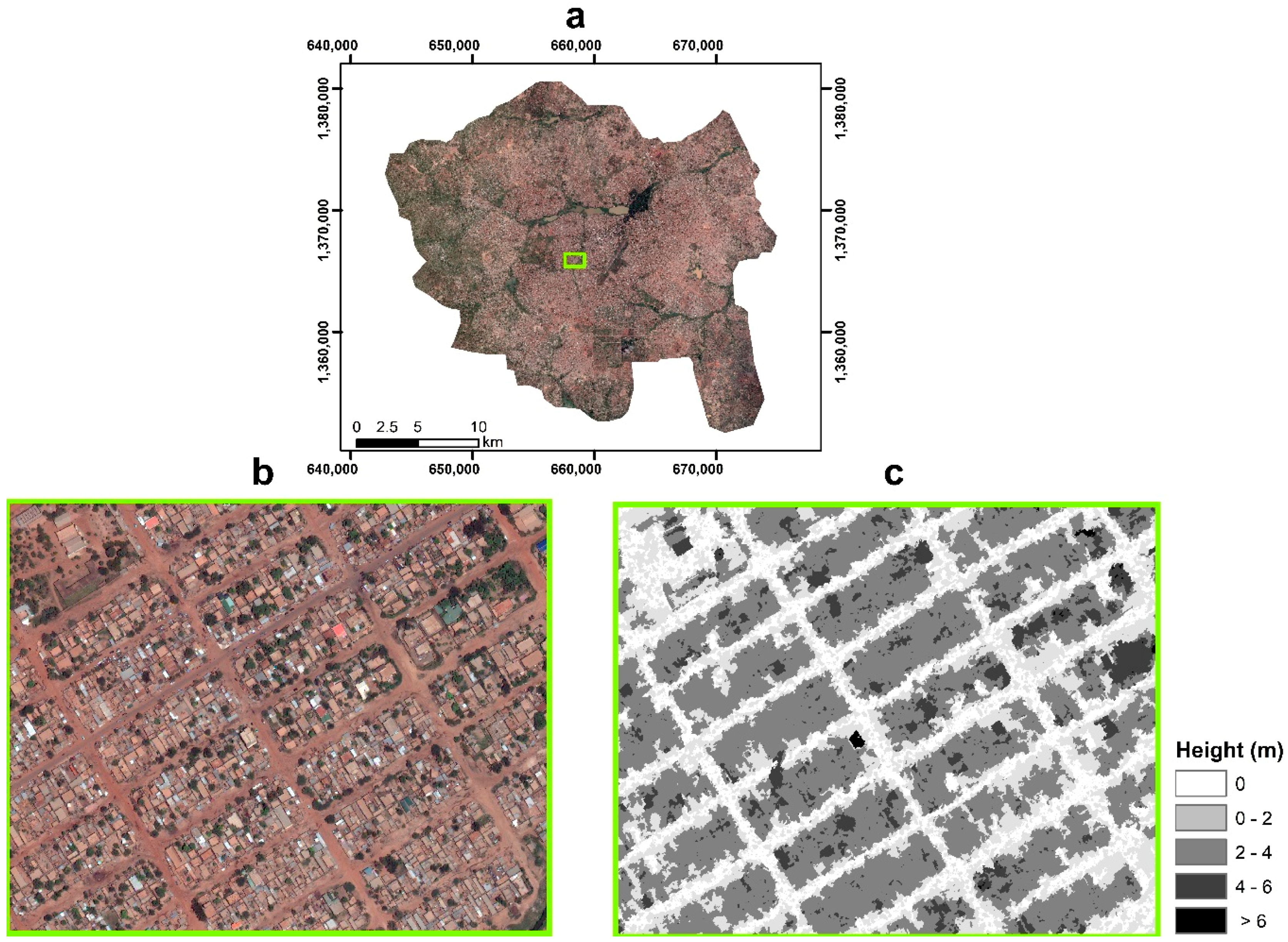
2.1. Study Area and Data

The study area covered the city of Ouagadougou, capital city of Burkina Faso in Sub-Saharan Africa (SSA). Ouagadougou comprises a complex and heterogenous urban landscape of planned and unplanned neighborhoods and buildings, of various sizes and materials [48]. The city has been undergoing extensive and partly unregulated urban growth (i.e., rural to urban migration) over the last decades [49,50]. To map the LULC of the city, we used a 4-band (R, G, B, NIR) WorldView-3 multispectral image (607 km2, Figure 1) from October 2015, and a normalized Digital Surface Model (nDSM) derived from stereo image acquisitions on the same image date. The native spatial resolution of the Worldview-3 imagery is 0.30 cm but was resampled at 0.50 cm by the provider. The value of the elevation information was critical, as the built-up characteristics were very hard to visually discriminate from bare soil and artificial ground surfaces, due to the presence of dust on rooftops and the use of similar construction materials for roofs and artificial ground surfaces. Thus, this challenging study site provided a good stress test for our methods.

2.2. Segmentation and Unsupervised Segmentation Parameter Optimization

The whole LULC classification framework was realized by employing and extending the semi-automated processing chain proposed by Grippa et al. [1]. The chain was implemented in a Jupyter Notebook format and integrated GRASS GIS functions with Python and R programming languages, framing a complete procedure from the input of initial datasets to final LULC map production. For segmentation, we utilized the RG algorithm implementation of GRASS GIS [51] with all four bands (VNIR) used as inputs. In the GRASS implementation, the TP ranges between 0 to 1, with 0 leading to the situation where each pixel represents a segment, while 1 unifies all image pixels in one object. As Böck et al. [52] pointed out, the USPO metrics are sensitive to the range of candidate segmentations used as input, so we empirically found a range that corresponded to cases of evident over- and under-segmentations to be used as minimum and maximum possible values, as commonly done in similar studies [18,53]. Thus, we evaluated 27 different segmentations starting with a TP of 4 and finishing at a TP of 31, guided by an incrementing step value of 1, as in previous studies, [54]. For reader convenience, all TP values were multiplied by 1000 in the illustrative and text materials.
To evaluate the quality of each of the different segmentations, we used the inter- and intra- segmentation heterogeneity metrics Moran’s I (MI) and Weighted Variance (WV), respectively. MI calculates the degree of spatial autocorrelation present in the values of nearby geographic features, and it was used in our case (and in many other USPO studies) to calculate how spectrally heterogeneous segments are, on average, from their neighbors (i.e., in terms of the mean segment values calculated for each spectral band). For this reason, it can provide a measure of “oversegmentation goodness”; Low MI values for a segmentation layer indicate low spatial autocorrelation between segment spectral values, suggesting that most segments belong to a different ground feature (with different spectral reflectance properties) than its neighbors. WV, on the other hand, describes the average spectral variability within segments (weighted by each segment’s area). WV can provide a measure of “undersegmentation goodness”; Low WV values indicate little internal variation in the spectral properties of segments, suggesting the segment does not contain a mixture of multiple ground features. MI and WV are given by:
  W V = i n a i v i i n a i  
  M I = n i n j n w i j z i z j M i n z i 2  
where for Equation (1), n is the number of segments, v i is the variance and a i the area for each segment, while in Equation (2), n is the number of segments, zi = xi x ¯ , x ¯ is the mean value of segment x, M = i = 1 n j = 1 n w i j and wij is the element of the matrix of spatial proximity M, which indicates the spatial connectivity for segments i and j [52,53].
To perform USPO, the oversegmentation and undersegmentation goodness values calculated for each segmentation layer need to be combined into a single value, e.g., through addition [38] or the F-measure [18]. We used the F-measure to combine MI and WV values in this study, as it was demonstrated to be less sensitive to excessive over- and undersegmentation than other combination approaches in Zhang et al. [39] and implemented in GRASS module “i.segment.uspo” [55]. To derive an F-measure from these two components, we first need to normalize them to a similar range (0–1) [38]:
M I n =   M I m a x     M I M I m a x     M I m i n ,
  W V n =   W V m a x     W V W V m a x     W V m i n ,  
where WVn is the normalized WV (or MI), WVmax is the maximum WV (or MI) value of all candidate segmentations, WVmin is the minimum WV (or MI) value of all candidate segmentations and WV is the WV (or MI) value of the current segmentation. The F-measure is a harmonic weighting of these two features:
  F o p t   =   ( 1   +   a 2 ) W V m a x     W V a 2     W V m a x     WV m i n ,  
where Fopt is the score of a candidate segmentation to be evaluated, ranging from 0 to 1, with higher values indicating higher quality; and a is the relative weight factor that assigns different significance to one metric over the other [18]. In our case we used a relative weight of 1, indicating equal weighting of the MI and WV components in calculating Fopt. The procedures were fully automated and parallelized due to the flexibility of GRASS GIS for applications including large raster datasets.

2.2.1. Global USPO

The conventional global USPO approach involves using either the whole image extent as input to the USPO procedure, or a representative subset [43]. Since our image was very large (20 GB), we used the latter method, as depicted in Figure 2. The selected subset (10 km2) contained planned, unplanned, and industrial built-up zones, with different kinds of vegetation, as well as bare soil, and thus, was deemed an appropriate candidate. The TP resulting from applying USPO to that region was 12, and we consequently used that value to segment all parts of the WorldView-3 image.

2.2.2. Spatially Partitioned Unsupervised Segmentation Parameter Optimization (SPUSPO)

As mentioned in the introduction, a global optimization of the USPO might not be appropriate due to the spatial heterogeneity within the image. As such, an alternative approach would be to partition the study area into several subsets, and to apply the optimization procedure locally in each subset. If the segmentation level selected as optimal by a global USPO calculation approach differs significantly from the segmentation level selected locally (i.e., through local USPO calculation in each partition of the study area), a spatially non-stationary process is taking place, and thus a global model might not be the best candidate to use. To investigate this phenomenon, we partitioned the image in three automated ways. The first two methods for partitioning were done using regularly-shaped rectangular tiles of predefined sizes, and the third partitioning method involved automated delineation using a cutline creating algorithm. The predefined partition was based on splitting the WorldView-3 image, into tiles of equal area and for most cases, equal geometry. The area of the rectangular image subsets for the first two partitioning approaches was 0.25 km2 (P1) and 0.12 km2 (P2), totaling to 2427 and 4887 subsets, respectively (Figure 3). Although the results of predefined partitioning can be fruitful for exploratory purposes, they suffer from edge effects at their borders. Since they are predefined and fixed in size, they arbitrarily partition the landscape, which can result in noisy/badly segmented objects along the boundaries of the rectangular subsets as artifacts (i.e., splitting building roofs or trees in half). To treat this issue, for the third and main partitioning approach (P3), we deployed a cutline creating algorithm using Laplacian zero-crossing edge detection [56,57,58], as implemented in the ‘i.cutlines’ module of GRASS GIS [59]. In that way, the created subsets would delineate the landscape in a more meaningful way, as they would follow linear patterns, such as roof edges and streets. The size of the cutline-created subsets can be decided by the user with respect to the application case. In our case, we created subsets closer to the P2 partition and as such, 4900 subsets were created. Examples of the different spatial partitioning methods are illustrated in Figure 3. In both global and local approaches, the minimum size of a created segment was preset at 14 pixels to avoid unnecessary oversegmentation.

2.2.3. Spatially Partitioned Unsupervised Segmentation Parameter Optimization (SPUSPO)

One of the merits of carrying out a localized approach is that it allows for decomposing a global process, into a wide set of useful information which is mappable. Since USPO was applied locally, a unique TP was produced for each spatial subset. The variation of the local TP from the single TP value of the global USPO can be quantified to assess the degree of spatial non-stationarity. If there would be no unexpected variation in the TP, that would suggest that a global approach is indeed adequate, ceteris paribus. Along with mapping the results, we proposed a Segmentation Parameter Stationarity Index (SPSI), which was loosely based on the Stationarity Index of Osborne et al. [60] to assess spatial non-stationarity in gaussian models:
  S P S I = I Q R ( T P L )   ( T P G + T P s t e p )     ( T P G T P s t e p )    
where T P G is the TP of the global USPO, T P s t e p is the step parameter of the USPO procedure, and I Q R ( T P L ) is the interquartile range of the distribution of the TP’s from a local approach. The interquartile range was used to mask outlier TP values that could emerge from random variation. Values equal to or smaller than 1 imply stationarity, as the variation of the local TPs is not exceeding what one would expect from a random process. Values higher than 1 indicate that there is significant spatial variation.

2.3. Land Use and Land Cover Classification

Ultimately, the segments were constructed with the aim of being labeled through a classification model. As such, another method to assess the local and global USPO methods is through the accuracy and performance of a LULC classification. The classification scheme and training data are presented below (Table 1). The training data were collected through random and stratified random sampling, and consisted of 2478 objects across the city, which were labeled through visual interpretation by two experts during the same period. The amount of training data was selected in such way that the addition of new data points did not significantly improve classification accuracy. Swimming pools were sampled manually due to their scarcity. To evaluate the results of the classification between the two methods, we used an expert-based manual delineation of Ouagadougou, based on building size and density [44] (Figure 4). In each one of these built-up types, we randomly sampled 150 points adding up to a total of 1650 points, and computed the Overall Accuracy (OA), as well as the F-score for each LULC class. No overlapping between training and testing data was allowed.
To classify the whole image, we computed several descriptive statistics for segments, based on the values of the pixels located within the segment, i.e., the values of each spectral band, NDVI values, and nDSM values (min, median, mean, max, range, 1st and 3rd quantiles and sum) as well as geometrical covariates (fractal dimension, perimeter, area, compactness). An Extreme Gradient Boosting (XGBoost, R 3.5.1) classifier was used as it was recently shown to outperform benchmark classifiers such as Support Vector Machine in VHR LULC classifications [14]. XGBoost is an ensemble of Classification and Regression Trees that is based in the principle of boosting [61]. The parameters of the algorithm were tuned through Bayesian Optimization [14,62], to ensure the quality of the results. Finally, we performed feature selection to reduce the computational burden and potentially increase the predictive capabilities of the model by deploying the popular Variable Selection with Random Forests (VSURF) algorithm, which is suited for tree-based classifiers such as XGBoost [63,64]. Out of the initial 59 features, 18 were selected by VSURF to build the most discriminant, redundancy-free model.

2.4. Segmentation Goodness Metrics

To evaluate the effect of SPUSPO on the segmentation of buildings, we compared the cutline-based segmentation and the global approach against reference data. In detail, we manually delineated 100 buildings that were randomly selected from the pool of training data used for the LULC classification. Finally, we computed the Area Fit Index (AFI) which is a commonly used joint index of over- and undersegmentation [31,32,53]:
  A F I = a r e a ( x i )   a r e a ( y i m a x )   a r e a ( x i )  
where xi is the reference object and yimax is the largest relevant segment intersecting xi. Values closer to 0 suggest a better segmentation, values > 0 imply oversegmentation whereas values < 0 undersegmentation.

2.5. Computational Requirements and Data Availability

The computing infrastructure used for the experiments consisted of two Intel® Xeon® CPU E5-2690 (2 processors of 2.90 GHz, 16 cores, 32 processing threads) and 96 GB of RAM. Segmenting the WorldView-3 image with a single TP parameter (tiled) required roughly 20 h of processing time while on average, a SPUSPO method required about 63 hours by exploiting the parallelization of the ‘i.segment.uspo’ module of GRASS [56]. The code, results and processed material is openly accessible in the following repository (https://zenodo.org/record/1341116#.W3FSUvZuJ_t) [65].

3. Results

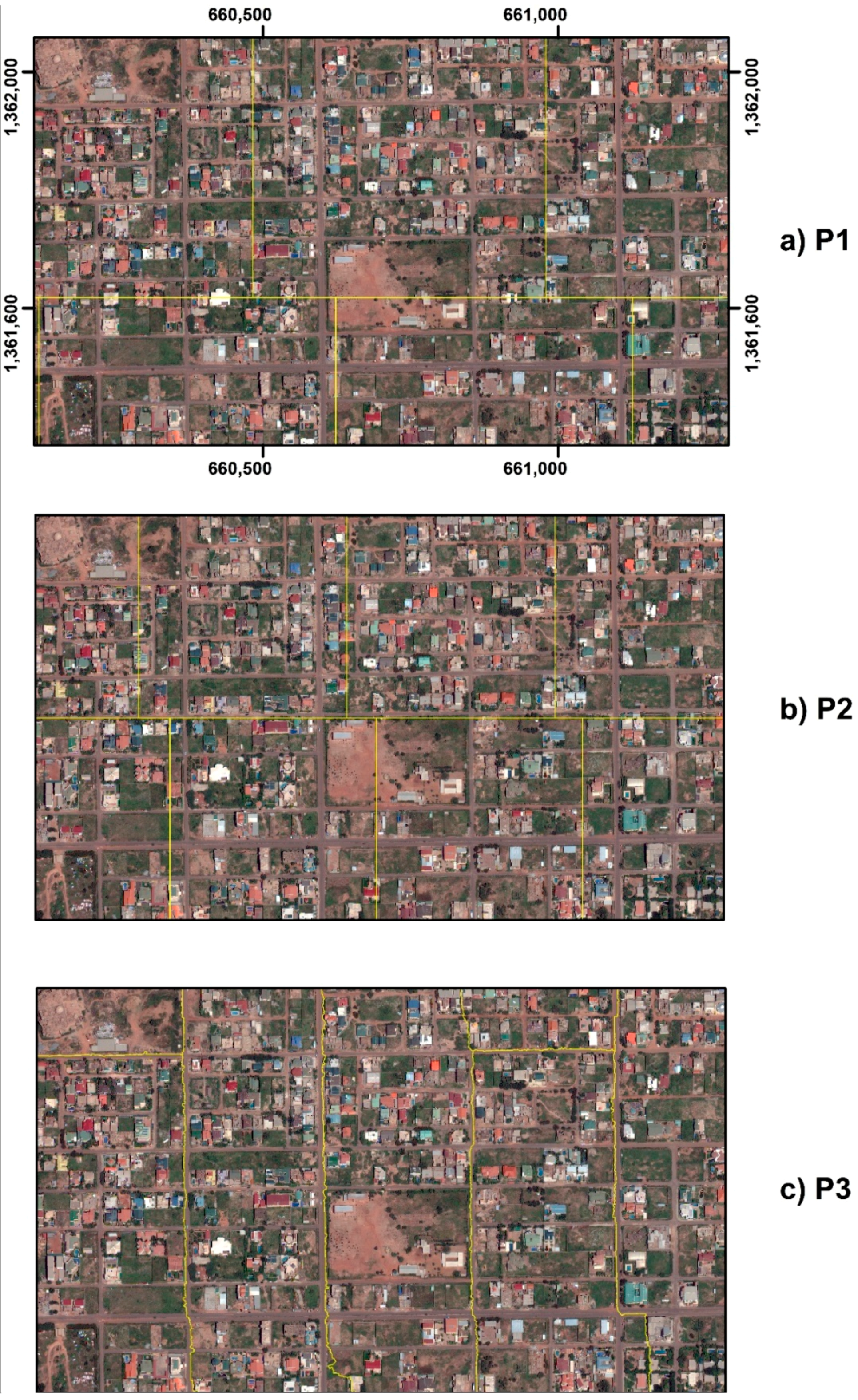
3.1. Threshold Parameter Variation

The spatial variation of the TP was a function of the size and geometry of the subsets used for local optimization. Figure 5 demonstrates that the variation follows patterns of the landscape. The locations where high TP values were selected as optimal were mainly clustered around unplanned, low elevated neighborhoods, whereas the locations where very low TP values were selected as optimal were mostly found in vegetated areas, potentially due to their unique spectral properties (high local variation in the NIR band). The local outputs of each metric used for the local USPO calculations can also be enlightening with respect to illustrating the level of spatial heterogeneity of the imagery. Figure 6 and Figure 7 confirm that MI and WV have an inverse relationship, with MI being decisive in optimization in the central and eastern regions of unplanned areas, and vice-versa. The SPSI value was 1.5 for P1, and 2 for P2 and P3, indicating a non-stationary variation in optimal TP values.
The variability of these parameters was also visualized in a set of boxplots in Figure 8. From this figure, the TP parameter variation is slightly smaller for the P1 approach than for the other two partitioning methods, possible because image partitions of P1 are larger than those of P2 and P3, and thus do not capture as much of the local heterogeneity in urban structure. Notably, when using smaller spatial partitions, MI tends to decrease (and WV tends to increase), which constitute the differences in TP among the different methods.

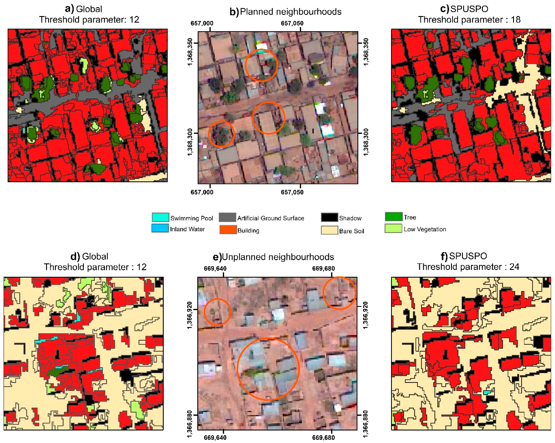
3.2. Land-Use Land-Cover Classification

The results of the LULC classification were found to be affected by the segmentation quality. Figure 9 and Figure 10 show case how SPUSPO could enhance classification accuracy by producing segments better fitting the local environment, in various areas in Ouagadougou. Figure 9 demonstrates that in both planned and unplanned regions, the improvement in classification results was mainly due to the cutlines segmentation, delineating the buildings in a less oversegmenting fashion, avoiding overestimation of built-up near the borders due to the inconsistent and “patchy” nature of the nDSM as a predictor, that does not closely follow built-up boundaries.
LULC classification based on SPUSPO was superior for vegetation and waterbodies of Ouagadougou. Figure 10 demonstrates cases of confusion between low and high vegetation, when using a global approach. Additionally, the misclassification of water as built-up is significantly less with SPUSPO. Notably, a scene might be segmented with intrinsically different thresholds (Figure 10f), which implies that the reason SPUSPO methods performed better is their incorporation of only the spatial information of the segmented region, and not information that comes from locations far away, which might not be useful at the local level.
The Overall Accuracy for the SPUSPO and global optimization based on the reference set was 90.5% and 89%, respectively. Moreover, the differences among them were statistically significant, based on a two-tailed McNemar’s test of similarity (p < 0.05). The local optimization was superior for most cases, both when concerning the OA and per-class evaluation metrics (Table 2). The largest improvements were found in the classification of inland water and shadows (+18% and +3% increase on the F1 score, respectively).
An additional, indirect way to assess the segmentation quality is to investigate the variable importance of the geometrical covariates. The geometrical covariates that were used in the classification model after VSURF feature selection took place were perimeter, area, and fractal dimension. Figure 11 illustrates the improved effect a local approach has on the importance of most of these variables, further supporting the merit of using SPUSPO. The interpretation of the results, refers to the gain in model accuracy when a feature is used in the splits of the XGBoost tree development. The importance of these covariates is varying, but in all cases, the local approach further enhances their predictive power for classification, since the segments fit better the variability of the local environment.

3.3. Segmentation Goodness Metrics

The results of the AFI for buildings are depicted in Table 3 through several descriptive statistics. As expected, the building objects were less over segmented with SPUSPO, because the parameter was spatially adapting to characteristics of each built-up neighborhood in Ouagadougou (Figure 12). The AFI values of the local method were consistently closer to zero compared to their counterpart, further promoting the use of this approach.

4. Discussion

The results suggested that the benefits of performing SPUSPO, are multiple. To start with, it allows for the local variations in spectral and spatial heterogeneity within an image to be incorporated into the segmentation parameter optimization approach, which is more intuitive because the optimization procedure is derived using the actual locations they are being applied to and not from locations situated afar. This supports the hypothesis that in large and heterogeneous areas, a single TP may be inadequate, as it is simply an average expression of several non-stationary processes. The results confirm prior analysis in another Sub-Saharan city of Dakar, where a semi-automated local approach outperformed classical optimization methods [54]. Moreover, several other studies have described how regionalized approaches can be of merit for urban, semi-rural, and agricultural environments [35,43,44]. Nonetheless, an important facet that has been neglected so far is how to partition the landscape in geographically large areas in conjunction with VHR imagery, and in the absence of reference data such as parcels or blocks. For a continuous LULC map, an appropriate delineation of the image is important, as it must be as adjustable to landscape patterns, such as streets or roofs, as much as possible to avoid/reduce edge effects. Although all local approaches showed they can be of merit, the cutline-based partition helped to specifically address these issues. Undertaking SPUSPO, produced higher classification accuracy than using a traditional global optimization method (+1.5% increase in OA). The results are confirmed further using AFI as a segmentation goodness metric, which showed that building segments from applying SPUSPO are less oversegmented than their global counterparts, with mean values of 0.28 and 0.36 for SPUSPO and global USPO, respectively. The analysis validated our initial hypothesis that the way we look at the data can produce significantly different results, and is related to the importance of appropriate spatial scale selection in geography, which was largely signified through the work of Woodcock and Strahler [66] and Fotheringham et al. [67]. Additionally, a local segmentation optimization approach is not only linked to traditional GEOBIA analysis, but might be needed in large scale applications where deep learning classification is coupled with segments to achieve better object delineation/extraction as demonstrated recently in References [68,69,70]. Another important piece of information that we can extract from these methods is the ability to map intermediate and final results, which can be enlightening both as a general understanding of how spatial processes operate in the local scale, but also how to calibrate segmentation parameters in further processing if an unsupervised multi-scale framework is selected [18]. The LULC products in SSA cities are often used as inputs for fine scale population modelling, land use, and spatial planning, and consequently, effective policy making, given the extreme scarcity of reference information [2,71,72]. This is significant for the outcome of our analyses because there was better prediction of most classes by the SPUSPO approach; it presents an additional motivation to partake of a local method to reduce error propagation in secondary models.
The main limitation of SPUSPO is the increased computational time and experimentation to detect a satisfactory spatial level to analyze image information, which can vary depending on the image resolution and study area, leading to a trade-off between computational requirements and performance. Therefore, more sophisticated methods are needed to help establish an efficient framework to fully exploit the benefits of local optimization. Ideally, in large and heterogeneous areas, a spatial partition should not suffer from edge effects and should meaningfully delineate the landscape with a certain degree of intra-homogeneity. Cutline partitioning satisfies both criteria to some extent, but its effectiveness can only be determined post-hoc, which increases the computational and time demands as several cutline partitions may need to be evaluated. More adequate methods that can focus in a priori determination of a suitable scale using image statistics, such as spatial dependency among regions [73], could be of benefit to achieve this, particularly in a multi-scale context. Other research should explore the potential of multi-resolution imagery to define operational partitions using top down approaches. For instance, a low-medium resolution LULC product can define homogeneous regions to apply SPUSPO using finer resolution imagery. Moreover, noise additive models could help in better establishing a comparative framework among different segmentation approaches, particularly for SAR or hyperspectral data [74]. A lot of the limitations that come with involving local methods, can be significantly reduced (i) by utilizing GRASS GIS, which is highly parallelized in the USPO optimization module and more notably, performs all the operations in a raster format and does not require vector conversion at any moment, dramatically boosting its effectiveness for large-scale computing; and (ii) invoking state-of-the-art segmentation algorithms, with respect to their computational efficiency, as recently shown by Gu et al. [75].

5. Conclusions

In this study, the optimization of a region-growing segmentation algorithm was attempted using a spatially varying parameter model, named SPUSPO. The whole framework was developed with a focus on automation and large-scale analysis of VHR imagery. The results validated our hypothesis that in large and heterogeneous areas, using only a single set of parameters to optimize the region-growing algorithm was inadequate. Employing as a case study, the city of Ouagadougou, it was demonstrated that undertaking local optimization methods was of merit and led to significantly better LULC classification results (+1.5% increase in OA), validated by a McNemar’s test of similarity. Moreover, at the segmentation level, building delineation was improved with a mean Area Fit Index of 0.28 and 0.36 for SPUSPO and global USPO, respectively. Moreover, the feature importance of geometrical covariates is recommended as an indirect measure to assess the quality of a segmentation. We demonstrated that geometrical features were more important and predictive when using local approaches. Finally, GRASS GIS was heavily utilized and is promoted as an open source tool to handle large volumes of data with advanced analysis techniques.

Author Contributions

S. Georganos wrote the manuscript and performed the analysis. M. Lennert developed the cutline algorithm. T. Grippa provided technical assistance and helped develop the experiments. B. Johnson, S. Vanhuysse and E. Wolff provided valuable feedback and comments during the internal revisions of the manuscript.

Acknowledgments

This work was supported by BELSPO (Belgian Science Policy Office) in the frame of the STEREO III program—project REACT (SR/00/337). We would also like to thank the three reviewers for their useful and insightful comments and recommendations which significantly improved the quality of the manuscript. WorldView3 data is copyrighted under the mention “©COPYRIGHT 2015 DigitalGlobe, Inc., Longmont CO USA 80503. DigitalGlobe and the DigitalGlobe logos are trademarks of DigitalGlobe, Inc. The use and/or dissemination of this data and/or of any product in any way derived there from are restricted. Unauthorized use and/or dissemination is prohibited”.

Conflicts of Interest

The authors declare no conflict of interest.

References

  1. Grippa, T.; Lennert, M.; Beaumont, B.; Vanhuysse, S.; Stephenne, N.; Wolff, E. An open-source semi-automated processing chain for urban object-based classification. Remote Sens. 2017, 9, 358. [Google Scholar] [CrossRef]
  2. Kabaria, C.W.; Molteni, F.; Mandike, R.; Chacky, F.; Noor, A.M.; Snow, R.W.; Linard, C. Mapping intra-urban malaria risk using high resolution satellite imagery: A case study of Dar es Salaam. Int. J. Health Geogr. 2016, 15, 26. [Google Scholar] [CrossRef] [PubMed]
  3. Linard, C.; Gilbert, M.; Snow, R.W.; Noor, A.M.; Tatem, A.J. Population distribution, settlement patterns and accessibility across Africa in 2010. PLoS ONE. 2012, 7, e31743. [Google Scholar] [CrossRef] [PubMed]
  4. Taubenbock, H.; Wurm, M.; Setiadi, N.; Gebert, N.; Roth, A.; Strunz, G.; Birkmann, J.; Dech, S. Integrating remote sensing and social science. In Proceedings of the IEEE Joint Urban Remote Sensing Event, Shanghai, China, 20–22 May 2009. [Google Scholar]
  5. Niehoff, D.; Fritsch, U.; Bronstert, A. Land-use impacts on storm-runoff generation: Scenarios of land-use change and simulation of hydrological response in a meso-scale catchment in SW-Germany. J. Hydrol. 2002, 267, 80–93. [Google Scholar] [CrossRef]
  6. Otukei, J.R.; Blaschke, T. Land cover change assessment using decision trees, support vector machines and maximum likelihood classification algorithms. Int. J. Appl. Earth Obs. Geoinf. 2010, 12, 27–31. [Google Scholar] [CrossRef]
  7. Manakos, I.; Braun, M. Land Use and Land Cover Mapping in Europe, 3rd ed.; Springer Nature: Heidelberg, Germany, 2014. [Google Scholar]
  8. Iizuka, K.; Johnson, B.A.; Onishi, A.; Magcale-Macandog, D.B.; Endo, I.; Bragais, M. Modeling Future Urban Sprawl and Landscape Change in the Laguna de Bay Area, Philippines. Land 2017, 6, 26. [Google Scholar] [CrossRef]
  9. Blaschke, T.; Hay, G.J.; Kelly, M.; Lang, S.; Hofmann, P.; Addink, E.; Queiroz Feitosa, R.; van der Meer, F.; van der Werff, H.; van Coillie, F.; et al. Geographic Object-Based Image Analysis—Towards a new paradigm. ISPRS J. Photogramm. Remote Sens. 2014, 87, 180–191. [Google Scholar] [CrossRef] [PubMed]
  10. Chen, G.; Weng, Q.; Hay, G.J.; He, Y. Geographic Object-based Image Analysis (GEOBIA): Emerging trends and future opportunities. GIScience Remote Sens. 2018, 55. [Google Scholar] [CrossRef]
  11. Gu, H.; Li, H.; Yan, L.; Liu, Z.; Blaschke, T.; Soergel, U. An object-based semantic classification method for high resolution remote sensing imagery using ontology. Remote Sens. 2017, 9, 329. [Google Scholar] [CrossRef]
  12. Blaschke, T. Object based image analysis for remote sensing. ISPRS J. Photogramm. Remote Sens. 2010, 65, 2–16. [Google Scholar] [CrossRef]
  13. Rasanen, A.; Rusanen, A.; Kuitunen, M.; Lensu, A. What makes segmentation good? A case study in boreal forest habitat mapping. Int. J. Remote Sens. 2013, 34, 8603–8627. [Google Scholar] [CrossRef] [Green Version]
  14. Georganos, S.; Grippa, T.; Vanhuysse, S.; Lennert, M.; Shimoni, M.; Wolff, E. Very high resolution object-based land use-land cover urban classification using extreme gradient boosting. IEEE Geosci. Remote Sens. Lett. 2018, 15, 607–611. [Google Scholar] [CrossRef]
  15. Ma, L.; Li, M.; Blaschke, T.; Ma, X.; Tiede, D.; Cheng, L.; Chen, Z.; Chen, D. Object-based change detection in urban areas: The effects of segmentation strategy, scale, and feature space on unsupervised methods. Remote Sens. 2016, 8, 761. [Google Scholar] [CrossRef]
  16. Srivastava, M.; Arora, M.K.; Raman, B. Selection of critical segmentation-A prerequisite for Object based image classification. In Proceedings of the 2015 National Conference on Recent Advances in Electronics & Computer Engineering (RAECE), Roorkee, India, 13–15 February 2015. [Google Scholar]
  17. Lowe, S.H.; Guo, X. Detecting an optimal scale parameter in object-oriented classification. IEEE J. Sel. Top. Appl. Earth Obs. Remote Sens. 2011, 4, 890–895. [Google Scholar] [CrossRef]
  18. Johnson, B.; Bragais, M.; Endo, I.; Magcale-Macandog, D.; Macandog, P. Image segmentation parameter optimization considering within- and between-segment heterogeneity at multiple scale levels: Test case for mapping residential areas using landsat imagery. ISPRS Int. J. Geo-Inform. 2015, 4, 2292–2305. [Google Scholar] [CrossRef]
  19. Gao, Y.A.N.; Mas, J.F.; Kerle, N.; Navarrete Pacheco, J.A. Optimal region growing segmentation and its effect on classification accuracy. Int. J. Remote Sens. 2011, 32, 3747–3763. [Google Scholar] [CrossRef]
  20. Yang, J.; Li, P.; He, Y. A multi-band approach to unsupervised scale parameter selection for multi-scale image segmentation. ISPRS J. Photogramm. Remote Sens. 2014, 94, 13–24. [Google Scholar] [CrossRef]
  21. Zhang, Q.; Huang, X.; Zhang, L. An energy-driven total variation model for segmentation and classification of high spatial resolution remote-sensing imagery. IEEE Geosci. Remote Sens. Lett. 2013, 10, 125–129. [Google Scholar] [CrossRef]
  22. Baatz, M.; Schape, A. Multiresolution Segmentation: An Optimization Approach for High Quality Multi-Scale Image Segmentation. 2000. Available online: https://www.semanticscholar.org/paper/Multiresolution-Segmentation-an-optimization-appro-Baatz-Sch%C3%A4pe/364cc1ff514a2e11d21a101dc072575e5487d17e (accessed on 20 December 2017).
  23. Grybas, H.; Melendy, L.; Congalton, R.G. A comparison of unsupervised segmentation parameter optimization approaches using moderate- and high-resolution imagery. GISci. Remote Sens. 2017, 54, 515–533. [Google Scholar] [CrossRef]
  24. Du, S.; Guo, Z.; Wang, W.; Guo, L.; Nie, J. A comparative study of the segmentation of weighted aggregation and multiresolution segmentation. GISci. Remote Sens. 2016, 53, 1–20. [Google Scholar] [CrossRef]
  25. Mesner, N.; Oštir, K. Investigating the impact of spatial and spectral resolution of satellite images on segmentation quality. J. Appl. Remote Sens. 2014, 8, 83696. [Google Scholar] [CrossRef] [Green Version]
  26. Zhong, Y.; Gao, R.; Zhang, L. Multiscale and multifeature normalized cut segmentation for high spatial resolution remote sensing imagery. IEEE Trans. Geosci. Remote Sens. 2016, 54, 6061–6075. [Google Scholar] [CrossRef]
  27. Duro, D.C.; Franklin, S.E.; Dube, M.G. A comparison of pixel-based and object-based image analysis with selected machine learning algorithms for the classification of agricultural landscapes using SPOT-5 HRG imagery. Remote Sens. Environ. 2012, 118, 259–272. [Google Scholar] [CrossRef]
  28. Zhang, H.; Fritts, J.E.; Goldman, S.A. Image segmentation evaluation: A survey of unsupervised methods. Comput. Vis. Image Underst. 2008, 110, 260–280. [Google Scholar] [CrossRef]
  29. Flanders, D.; Hall-Beyer, M.; Pereverzoff, J. Preliminary evaluation of ecognition object-based software for cut block delineation and feature extraction. Can. J. Remote Sens. 2003, 29, 441–452. [Google Scholar] [CrossRef]
  30. Belgiu, M.; Drăgut, L. Random forest in remote sensing: A review of applications and future directions. ISPRS J. Photogramm. Remote Sens. 2016, 114, 24–31. [Google Scholar] [CrossRef]
  31. Clinton, N.; Holt, A.; Scarborough, J.; Yan, L.; Gong, P. Accuracy assessment measures for object-based image segmentation goodness. Photogramm. Eng. Remote Sens. 2010, 76, 289–299. [Google Scholar] [CrossRef]
  32. Costa, H.; Foody, G.M.; Boyd, D.S. Supervised methods of image segmentation accuracy assessment in land cover mapping. Remote Sens. Environ. 2018, 205, 338–351. [Google Scholar] [CrossRef]
  33. Belgiu, M.; Drǎguţ, L. Comparing supervised and unsupervised multiresolution segmentation approaches for extracting buildings from very high resolution imagery. ISPRS J. Photogramm. Remote Sens. 2014, 96, 67–75. [Google Scholar] [CrossRef] [PubMed]
  34. Drǎguţ, L.; Tiede, D.; Levick, S.R. ESP: A tool to estimate scale parameter for multiresolution image segmentation of remotely sensed data. Int. J. Geogr. Inf. Sci. 2010, 24, 859–871. [Google Scholar] [CrossRef]
  35. Kavzoglu, T.; Erdemir, M.Y.; Tonbul, H. Classification of semiurban landscapes from very high-resolution satellite images using a regionalized multiscale segmentation approach. J. Appl. Remote Sens. 2017, 11, 35016. [Google Scholar] [CrossRef]
  36. Johnson, B.; Xie, Z. Unsupervised image segmentation evaluation and refinement using a multi-scale approach. ISPRS J. Photogramm. Remote Sens. 2011, 66, 473–483. [Google Scholar] [CrossRef]
  37. Dragut, L.; Csillik, O.; Eisank, C.; Tiede, D. Automated parameterisation for multi-scale image segmentation on multiple layers. ISPRS J. Photogramm. Remote Sens. 2014, 88, 119–127. [Google Scholar] [CrossRef] [PubMed]
  38. Espindola, G.M.; Camara, G.; Reis, I.A.; Bins, L.S.; Monteiro, A.M. Parameter selection for region-growing image segmentation algorithms using spatial autocorrelation. Int. J. Remote Sens. 2006, 27, 3035–3040. [Google Scholar] [CrossRef]
  39. Zhang, X.; Feng, X.; Xiao, P.; He, G.; Zhu, L. Segmentation quality evaluation using region-based precision and recall measures for remote sensing images. ISPRS J. Photogramm. Remote Sens. 2015, 102, 73–84. [Google Scholar] [CrossRef]
  40. Grippa, T.; Lennert, M.; Beaumont, B.; Vanhuysse, S.; Stephenne, N.; Wolff, E. An open-source semi-automated processing chain for urban obia classification. In Proceedings of the GEOBIA 2016: Solutions and Synergies, Enschede, The Netherlands, 14–16 September 2016. [Google Scholar]
  41. Li, M.; Ma, L.; Blaschke, T.; Cheng, L.; Tiede, D. A systematic comparison of different object-based classification techniques using high spatial resolution imagery in agricultural environments. Int. J. Appl. Earth Obs. Geoinf. 2016, 49, 87–98. [Google Scholar] [CrossRef]
  42. Ma, L.; Li, M.; Ma, X.; Cheng, L.; Du, P.; Liu, Y. A review of supervised object-based land-cover image classification. ISPRS J. Photogramm. Remote Sens. 2017, 130, 277–293. [Google Scholar] [CrossRef]
  43. Cánovas-García, F.; Alonso-Sarría, F. A local approach to optimize the scale parameter in multiresolution segmentation for multispectral imagery. Geocarto Int. 2015, 30, 937–961. [Google Scholar] [CrossRef]
  44. Grippa, T.; Georganos, S.; Vanhuysse, S.G.; Lennert, M.; Wolff, E. A local segmentation parameter optimization approach for mapping heterogeneous urban environments using VHR imagery. Remote Sens. Technol. Appl. Urban Environ. II 2017, 10431. [Google Scholar] [CrossRef] [Green Version]
  45. Gorelick, N.; Hancher, M.; Dixon, M.; Ilyushchenko, S.; Thau, D.; Moore, R. Remote sensing of environment google earth engine: Planetary-scale geospatial analysis for everyone. Remote Sens. Environ. 2017, 202, 18–27. [Google Scholar] [CrossRef]
  46. Tobler, W.R. A computer movie simulating urban growth in the detroit region. Econ. Geogr. 1970, 46, 234–240. [Google Scholar] [CrossRef]
  47. Neteler, M.; Bowman, M.H.; Landa, M.; Metz, M. GRASS GIS: A multi-purpose open source GIS. Environ. Model. Softw. 2012, 31, 124–130. [Google Scholar] [CrossRef] [Green Version]
  48. Grippa, T.; Georganos, S.; Zarougui, S.; Bognounou, P.; Diboulo, E.; Forget, Y.; Lennert, M.; Vanhuysse, S.; Mboga, N.; Wolff, E. Mapping urban land use at street block level using open street map, Remote Sensing Data, and Spatial Metrics. ISPRS Int. J. Geo-Inform. 2018, 7, 246. [Google Scholar] [CrossRef]
  49. United Nations. World Urbanization Prospects: The 2014 Revision, Highlights, 3rd ed.; Population Division, United Nations: New York, NY, USA, 2014.
  50. Schug, F.; Okujeni, A.; Hauer, J.; Hostert, P.; Nielsen Jonas Øand van der Linden, S. Mapping patterns of urban development in Ouagadougou, Burkina Faso, using machine learning regression modeling with bi-seasonal Landsat time series. Remote Sens. Environ. 2018, 210, 217–228. [Google Scholar] [CrossRef]
  51. Momsen, E.; Metz, M.; GRASS Development TEAM. Module i.segment 2015. Available online: https://grass.osgeo.org/grass75/manuals/i.segment.html (accessed on 1 August 2018).
  52. Böck, S.; Immitzer, M.; Atzberger, C. On the objectivity of the objective function—Problems with unsupervised segmentation evaluation based on global score and a possible remedy. Remote Sens. 2017, 9, 769. [Google Scholar] [CrossRef]
  53. Georganos, S.; Lennert, M.; Grippa, T.; Vanhuysse, S.; Johnson, B.; Wolff, E. Normalization in unsupervised segmentation parameter optimization: A solution based on local regression trend analysis. Remote Sens. 2018, 10, 222. [Google Scholar] [CrossRef]
  54. Georganos, S.; Grippa, T.; Lennert, M.; Vanhuysse, S.G.; Wolff, E. SPUSPO: Spatially Partitioned Unsupervised Segmentation Parameter Optimization for Efficiently Segmenting Large Heteregeneous Areas. In Proceedings of the 2017 Conference on Big Data from Space (BiDS’17), Toulouse, France, 28–30 November 2017. [Google Scholar]
  55. Lennert, M.; GRASS Development TEAM. Module i.segment.uspo 2017. Available online: https://grass.osgeo.org/grass74/manuals/addons/i.segment.uspo.html (accessed on 1 August 2018).
  56. Körting, T.S.; Castejon, E.F.; Fonseca, L.M.G. The divide and segment method for parallel image segmentation. In Proceedings of the International Conference on Advanced Concepts for Intelligent Vision Systems, Antwerp, Belgium, 18–21 September 2013. [Google Scholar]
  57. Soares, A.R.; Körting, T.S.; Fonseca, L.M.G. Improvements of the divide and segment method for parallel image segmentation. Rev. Bras. Cartogr. 2016, 68. [Google Scholar]
  58. Satnik, D.; GRASS Development TEAM. Module i.zc 2016. Available online: https://grass.osgeo.org/grass70/manuals/i.zc.html (accessed on 1 August 2018).
  59. Lennert, M.; GRASS Development TEAM. Module i.cutlines 2018. Available online: https://grass.osgeo.org/grass74/manuals/addons/i.cutlines.html (accessed on 1 August 2018).
  60. Osborne, P.E.; Foody, G.M.; Suárez-Seoane, S. Non-stationarity and local approaches to modelling the distributions of wildlife. Divers. Distrib. 2007, 13, 313–323. [Google Scholar] [CrossRef]
  61. Chen, T.; Guestrin, C. XGBoost: Reliable large-scale tree boosting system. arXiv, 2016. [Google Scholar] [CrossRef]
  62. Xia, Y.; Liu, C.; Li, Y.; Liu, N. A boosted decision tree approach using Bayesian hyper-parameter optimization for credit scoring. Expert Syst. Appl. 2017, 78, 225–241. [Google Scholar] [CrossRef]
  63. Genuer, R.; Poggi, J.M.; Tuleau-Malot, C. VSURF: An R Package for variable selection using random forests. R J. 2015, 7, 19–33. [Google Scholar]
  64. Georganos, S.; Grippa, T.; Vanhuysse, S.; Lennert, M.; Shimoni, M.; Kalogirou, S.; Wolff, E. Less is more: Optimizing classification performance through feature selection in a very-high-resolution remote sensing object-based urban application. GISci. Remote Sens. 2017, 221–242. [Google Scholar] [CrossRef]
  65. Georganos, S.; Grippa, T.; Lennert, M.; Johnson, B.A.; Vanhuysse, S.; Wolff, E. SPUSPO: Spatially Partitioned Unsupervised Segmentation Parameter Optimization for Efficiently Segmenting Large Heterogeneous Areas. Available online: https://zenodo.org/record/1341116#.W5S1oVKtZS0 (accessed on 31 August 2018).
  66. Woodcock, C.E.; Strahler, A.H. The factor of scale in remote sensing. Remote Sens. Environ. 1987, 21, 311–332. [Google Scholar] [CrossRef]
  67. Fotheringham, A.S.; Brunsdon, C.; Charlton, M. Geographically weighted regression: The analysis of spatially varying relationships. Am. J. Agric. Econom. 2004, 86, 554–556. [Google Scholar] [CrossRef]
  68. Liu, T.; Abd-elrahman, A.; Jon, M.; Wilhelm, V.L.; Liu, T.; Abd-elrahman, A.; Jon, M.; Wilhelm, V.L. Comparing fully convolutional networks, random forest, support vector machine, and patch-based deep convolutional neural networks for object-based wetland mapping using images from small unmanned aircraft system. GISci. Remote Sens. 2018, 55, 243–264. [Google Scholar] [CrossRef]
  69. Liu, T.; Abd-Elrahman, A. Deep convolutional neural network training enrichment using multi-view object-based analysis of Unmanned Aerial systems imagery for wetlands classification. ISPRS J. Photogramm. Remote Sens. 2018, 139, 154–170. [Google Scholar] [CrossRef]
  70. Marmanis, D.; Schindler, K.; Wegner, J.D.; Galliani, S.; Datcu, M.; Stilla, U. Classification with an edge: Improving semantic image segmentation with boundary detection. ISPRS J. Photogramm. Remote Sens. 2018, 135, 158–172. [Google Scholar] [CrossRef] [Green Version]
  71. Linard, C.; Tatem, A.J.; Gilbert, M. Modelling spatial patterns of urban growth in Africa. Appl. Geogr. 2013, 44, 23–32. [Google Scholar] [CrossRef] [PubMed] [Green Version]
  72. Sandborn, A.; Engstrom, R.N. Determining the Relationship between Census Data and Spatial Features Derived From High-Resolution Imagery in Accra, Ghana. IEEE J. Sel. Top. Appl. Earth Obs. Remote Sens. 2016, 9, 1970–1977. [Google Scholar] [CrossRef]
  73. Ming, D.; Li, J.; Wang, J.; Zhang, M. Scale parameter selection by spatial statistics for GeOBIA: Using mean-shift based multi-scale segmentation as an example. ISPRS J. Photogramm. Remote Sens. 2015, 106, 28–41. [Google Scholar] [CrossRef]
  74. Yuan, Q.; Zhang, L.; Shen, H. Hyperspectral image denoising employing a spectral-spatial adaptive total variation model. IEEE Trans. Geosci. Remote Sens. 2012, 50, 3660–3677. [Google Scholar] [CrossRef]
  75. Gu, H.; Han, Y.; Yang, Y.; Li, H.; Liu, Z.; Soergel, U.; Blaschke, T.; Cui, S. An efficient parallel multi-scale segmentation method for remote sensing imagery. Remote Sens. 2018, 10, 590. [Google Scholar] [CrossRef]
Figure 1. (a) Study area extent illustrated from a WorldView-3 RGB composite of Ouagadougou, (b) a typical built-up neighborhood of Ouagadougou and (c) Normalized Digital Surface Model for the region.
Remotesensing 10 01440 g001
Figure 2. Subset of the WorldView-3 imagery (~10 km2) where the RG’s TP was optimized for use in the whole image. The selected area contains a distribution of land cover classes representative of the whole study area.
Remotesensing 10 01440 g002
Figure 3. Partitioning the WorldView-3 image into spatial subsets for local USPO optimization. (a) Delineation by 0.250 km2 area tiles, (b) delineation by 0.125 km2 area tiles and (c) delineation based on zero crossing cutline algorithm.
Remotesensing 10 01440 g003
Figure 4. Morphological delineation of Ouagadougou based on built-up size and density categories.
Remotesensing 10 01440 g004
Figure 5. Spatial variation of the threshold parameter (TP) across Ouagadougou. (a) WorldView-3 RGB composite, partitioning by (b) P1 (c) P2 and (d) P3 approaches, respectively. The TP controls the average size of the created segments.
Remotesensing 10 01440 g005
Figure 6. Spatial variation of weighted variance (WV) across Ouagadougou. (a) WorldView-3 RGB composite, partitioning by (b) P1, (c) P2 and (d) P3 approaches, respectively. High values of WV indicate large intra-segment variability while low values describe more homogenous objects.
Remotesensing 10 01440 g006
Figure 7. Spatial variation of Moran’s I (MI) values across Ouagadougou. (a) WorldView-3 RGB composite, partitioning by (b) P1 (c) P2 and (d) P3 approaches, respectively. The higher the MI value, the stronger the effect of spatial autocorrelation between a created segment and its neighbors.
Remotesensing 10 01440 g007
Figure 8. Boxplots demonstrating the variability of (a) the TP, (b) MI and (c) WV for the different partitioning approaches (P1, P2, P3).
Remotesensing 10 01440 g008
Figure 9. Example of the LULC map classification in a planned and unplanned built-up area. (a) LULC classification with a global approach in a planned neighborhood, (b) RGB Pleiades Composite, (c) LULC classification with a cutline approach in an unplanned neighborhood, and (d) LULC classification with a global approach in a planned neighborhood, (e) RGB Pleiades Composite, (f) LULC classification with a cutline approach in an unplanned neighborhood.
Remotesensing 10 01440 g009
Figure 10. Example of the LULC map classification in a vegetated regions and inland water bodies. (a) LULC classification with a global approach in a forested area, (b) RGB Pleiades Composite, (c) LULC classification with a cutline approach in a forested area, (d) LULC classification with a global approach in water bodies, (e) RGB Pleiades Composite, and (f) LULC classification with a cutline approach in water bodies.
Remotesensing 10 01440 g010
Figure 11. Feature importance of geometrical covariates, as derived from an XGBoost classifier, for the global and cutline segmentation-based approaches, respectively. The method used to derive importance is the gain in accuracy.
Remotesensing 10 01440 g011
Figure 12. Example segmentations of buildings in Ouagadougou. Red color indicates segments created by a global approach, while green color indicates segments coming from SPUSPO. The decrease of over segmentation is evident in most cases, as the parameters are derived from neighboring locations, better fitting the data structure.
Remotesensing 10 01440 g012
Table 1. Training objects for each LULC class and method.
LULCDescriptionTraining Set Size
Buildings (BU) 400
Swimming Pool (SP) 179
Artificial Ground Surface (AS)Asphalt, concrete, semi-built-up constructions216
Bare Soil (BS) 399
Tree (TR) 191
Low Vegetation (LV)Grass, bushes, dry vegetation702
Inland Water (IW)Lakes, ponds, rivers, wetlands205
Shadow (SH) 186
Table 2. Precision, Recall and F-score metrics for each LULC class with SPUSPO and global USPO, respectively.
PrecisionRecallF1
ClassSPUSPOGlobalSPUSPOGlobalSPUSPOGlobal
Building0.930.930.940.930.940.93
Artificial Ground Surface0.830.830.880.860.850.84
Bare Soil0.880.840.870.870.880.86
Tree0.810.810.910.930.850.87
Low veg0.940.940.890.860.910.90
Inland Water0.860.730.660.470.750.57
Shadow0.940.900.950.950.950.92
Table 3. Area Fit Index for building objects in Ouagadougou. Values closer to 0 suggest a better segmentation, values > 0 imply over segmentation while values < 0 under segmentation.
Descriptive StatisticsArea Fit Index (AFI)
SPUSPOGlobal
1st0.040.11
Median0.220.38
Mean0.280.36
3rd 0.530.62

