Multi-Temporal Satellite Images on Topsoil Attribute Quantification and the Relationship with Soil Classes and Geology

Abstract

The mapping of soil attributes provides support to agricultural planning and land use monitoring, which consequently aids the improvement of soil quality and food production. Landsat 5 Thematic Mapper (TM) images are often used to estimate a given soil attribute (i.e., clay), but have the potential to model many other attributes, providing input for soil mapping applications. In this paper, we aim to evaluate a Bare Soil Composite Image (BSCI) from the state of São Paulo, Brazil, calculated from a multi-temporal dataset, and study its relationship with topsoil properties, such as soil class and geology. The method presented detects bare soil in satellite images in a time series of 16 years, based on Landsat 5 TM observations. The compilation derived a BSCI for the agricultural sites (242,000 hectare area) characterized by very complex geology. Soil properties were analyzed to calibrate prediction models using 740 soil samples (0–20 cm) collected of the area. Partial least squares regression (PLSR) based on the BSCI spectral dataset was performed to quantify soil attributes. The method identified that a single image represents 7 to 20% of bare soil while the compilation of the multi-temporal dataset increases to 53%. Clay content had the best soil attribute prediction estimates (R² = 0.75, root mean square error (RMSE) = 89.84 g kg⁻¹, and accuracy = 74%). Soil organic matter, cation exchange capacity and sandy soils also achieved moderate predictions. The BSCI demonstrates a strong relationship with legacy geological maps detecting variations in soils. From a single composite image, it was possible to use spectroscopy to evaluate several environmental parameters. This technique could greatly improve soil mapping and consequently aid several applications, such as land use planning, environmental monitoring, and prevention of land degradation, updating legacy surveys and digital soil mapping.

1. Introduction

The FAO (Food and Agriculture Organization) estimates that the world population will increase from 7.3 billion to approximately 9 billion by 2050. Therefore, food production needs to increase by about 70% to feed the population in 2050 [1]. However, arable soil areas are decreasing due to the anthropogenic impact of degradation and urbanization. Poor soil management practices will threaten its capacity to provide soil resources, and possibly not enhance climate change policy [2]. Regarding sustainable soil use, different methodologies depend on explicit spatial information, which is essential to providing adequate soil and crop management, producing quality food without impacting environmental health [3].

Spatial variation of chemical and physical properties influences soil and crop management efficiency. Variability in soil properties can cause heterogeneous crop growth, can compromise agronomic prescription efficiency, and may alter crop production capacity [4,5,6,7]. Understanding the magnitude and patterns of spatial variability for soil properties is fundamental to management practices regarding fertilizer application, the design of field research programs and other soil-dependent activities.

A recent development, reported by Rossel and Buoma [8], demonstrated the importance of remote sensing (RS) for soils and agriculture. The information retrieved from Visible (Vis), Near Infrared (NIR) and Shortwave Infrared (SWIR) can be employed to calibrate site-specific datasets, which describe the relationship between spatio-temporal and quantitative soil information changes over large areas [9]. The RS satellite captures the electromagnetic energy reflected from the Earth’-s surface, which relates to physical and chemical soil surface properties, such as the topsoil matrix [9,10]. In other words, it captures the spectral reflectance fingerprint related to soil characteristics.

Multispectral sensors, such as the free access to Landsat imagery, have provided global coverage over time [11], supplying up-to-date information to the scientific community for field management studies and decision-making insights on arable lands spread worldwide. Additionally, Landsat provides information that can be used for a range of studies and interpretations [12]. In a global study, Ying et al. [13] observed the land use changes from 2000 to 2012 caused by natural resource extraction with RS and ground reference information. White et al. [14] and Hermosilla et al. [15] used RS data on a nationwide scale to support mapping and monitoring of forest ecosystems over Canada.

Among the soil mapping techniques, Digital Soil Mapping and Modeling (DSMM) have provided reliable and cost-effective information. DSMM is an approach that integrates soil and environmental datasets. However, there is no universal solution that fits all regions, as it requires merging aspects related to geographical and pedological expertise, sampling setup, spatial scale, incorporation of legacy data, and quantitative methods [16]. The set of soil data and covariates are often the limiting factor in model calibration [17]. Since DSMM involve soil data collection, it should be conducted at a regional or local level, consistent with its use and application [12], and as such, it may offer distinct improvements to conventional soil survey.

Furthermore, there has been increased the usage of the bare soil surface as a covariate for soil mapping and modeling in the RS and Digital Soil Map community [18]. Many authors have used different strategies to extract bare soil from satellite images and map its characteristics [19,20,21,22,23]. A single image is not enough to detect large surfaces, but fragmented information has proved effective in retrieving the relationship between soil spectral surface and soil attributes [19]. Over the years, novel methodologies of bare soil detection have improved, evolving into multi-temporal approaches to obtain larger areas of bare soil surfaces. Shabou et al. [20] detected bare soil pixels from images using the relationship between clay content and the MID-Infrared profile of four images. These authors combined the soil surface of one image with ordinary co-kriging to produce a soil clay content map for central Tunisia, Africa.

Demattê et al. [21] applied a fusion technique with five images to create a bare soil mosaic, which increased the bare soil coverage of the area from 36% (single image) to 75% and enabled mapping of the topsoil texture. Diek et al. [22] obtained 90% coverage for the Swiss Plateau (Switzerland) using 5 years of Landsat imagery and the Barest Soil Composite technique. The information was subsequently employed to map sand, silt, clay, and organic matter at the study site. Rogge et al. [23] developed the Soil Composite Mapping Processor (SCMaP) as an approach to overcome limited soil exposure and map soil characteristics in Germany.

The Piracicaba region in central São Paulo, Brazil, is characterized by complex relief, with high variability in soils formed by different parent materials. Soil image information is important for this region due to agribusiness intensification of the sugar and bioenergy industries. Thus, there is a specific time-window for satellite sensor monitoring of bare soil because of the crop cultivation during the year. The bare soil information could be used to calibrate models and map topsoil attributes. Furthermore, the integration of multi-temporal images would be beneficial to improving soil coverage and creating a single composite image dataset. Our hypothesis is that the retrieval of this unique information could be related to soil spatial variability. This study aims to create a multi-temporal Bare Soil Composite Image (BSCI) and verify its usefulness in the mapping of soil properties, and the relationship with soil classes and geology. The relationship with soil mineralogy, color and clay fraction presented in legacy maps is also established. This study intends to show that image spectroscopy can be applied to several environmental parameters.

2. Materials and Methods

The proposed method is to assess bare soil, by masking green vegetation and crop residue targets from Landsat images. The compilation of time series images creates a BSCI, providing soil surface reflectance data for modeling topsoil properties (Figure 1).

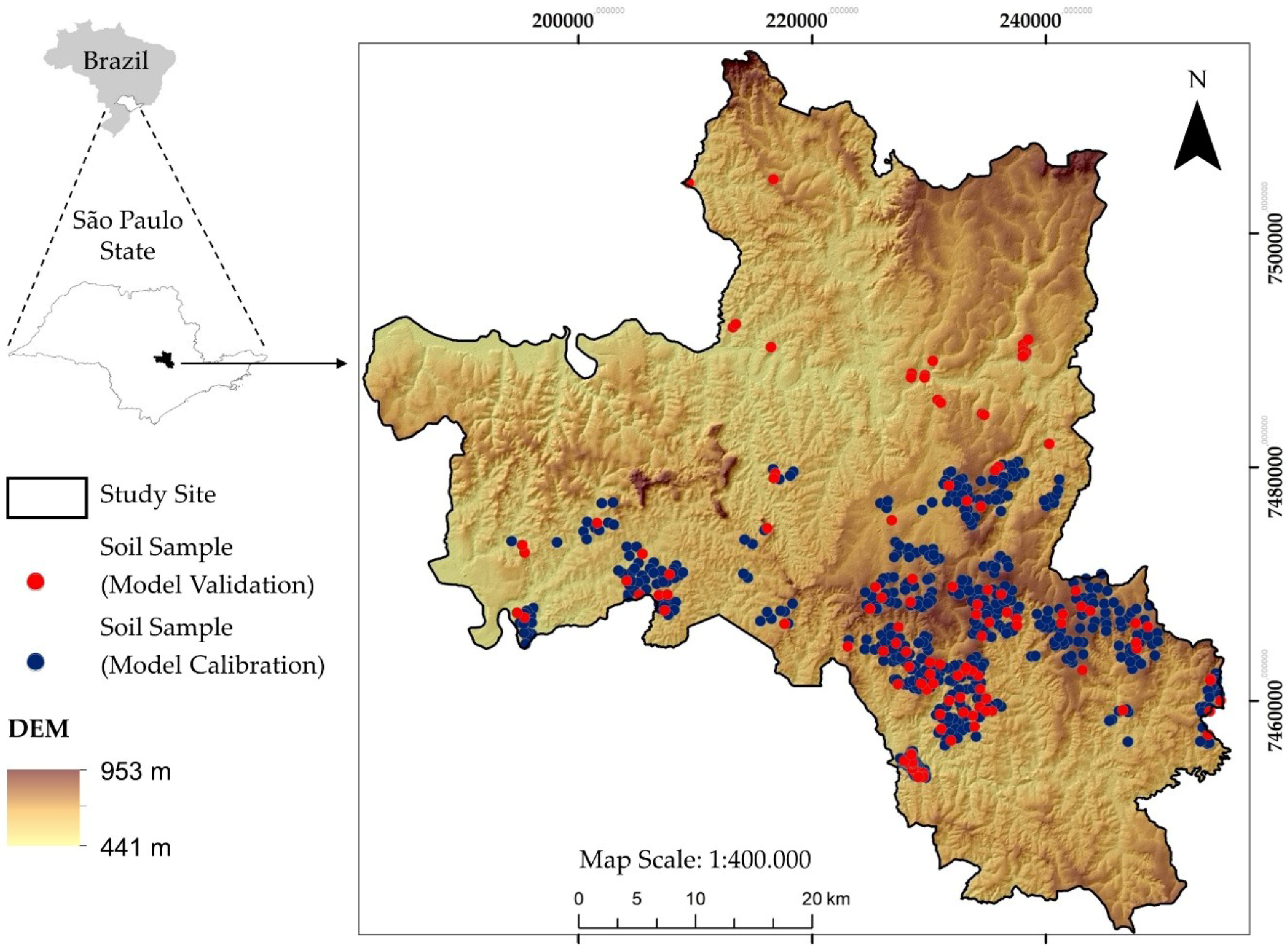
2.1. Study Site and Soil Samples

The 242,000 hectare study site covers eight cities (Piracicaba, Saltinho, Mombuca, Rio das Pedras, Iracemápolis, Charqueada, Capivari and Rafard) in central São Paulo State, Brazil (Figure 2). The region is classified as humid subtropical on the Koppen classification system and characterized by dry winter (May–September) and hot rainy summers (October–April) [24]. The average annual rainfall is approximately 1273 mm year⁻¹ and the average annual temperature is 24 °C. The landscape is gently undulating and rolling uplands, with slopes between 0 and 42%.

Agriculture is the predominant land use in the area, with plowing being a common practice in preparation for sowing. The plowing activity break up and turn over soil in a depth of 0 to 20 cm, it keeps the surface layer homogenous. Thus, topsoil samples (Epipedon) were collected in toposequence scheme with an auger (0–20 cm). The toposequence was designed using several parameters as a variation of soil type [25], geology [26], and Digital Elevation Model (DEM) [27] observations (Figure 3). The topsoil samples corresponded to 740 points, which represent the variability of the entire area (Figure 2). Sampling sites were geo-referenced using global positioning system (GPS).

The soil samples were oven-dried for 48 h at 50 °C, ground and sieved (2 mm mesh) to analyze chemical and particle size properties according to the Brazilian Soil Classification System [28]. The densimeter method was used to obtain soil particle size, coarse and fine sand, silt, and clay [29]. The following chemical attributes were determined according to Raij et al. [30]: exchangeable bases (Ca²⁺, Mg²⁺, and K⁺), available phosphorus and soil organic carbon. From the chemical attributes, the sum of bases (SB), cation exchange capacity (CEC), base saturation (V%) and aluminum saturation (m%) were calculated.

At the study site, the geology (Figure 3a) includes fine to medium, reddish, silty-clay sandstone of the Botucatu and Pirambóia Formation and dike elements of basic intrusive diabase rocks of the Serra Geral Formation. There are places where the Pirambóia Formation covers the Corumbataí Formation, presenting the incidence of chert marks of the contact between these two Formations. The Irati Formation (Passa Dois Group) arises on the top of sandy deposits where the relief is gently undulating to flat, but as it approaches the hillshade areas the diabase rocks of Serra Geral formation occur (Figure 3b). The diabase rocks also ascend between the siltstones that are the predominant lithology of the Itararé and Tatuí Formation (Tubarão group).

The high soil variability is mainly due to the complexity and diversity of the parent material of the neo-Cenozoic surficial deposits of various textures (Figure 3b). Here, the soil types were classified at the suborder level according to the Brazilian Soil Classification System (SiBCS) [28]. The corresponding Soil Taxonomy [31], and World Reference Base [32] classes are shown in

Table 1. Soil suborders according to the Brazilian Classification System [28], and corresponding Soil Taxonomy [31], and Word Reference Base [32].

SiBCS Classification	Soil Taxonomy Classification	WRB Classification
Cambissolo Háplico (CX)	Udepts	Cambisol
Gleissolo Háplico (GX)	Aquents	Gleysol
Latossolo Vermelho (LV)	Udox	Ferralsol
Latossolo Vermelho-Amarelo (LVA)	Udox	Ferralsol
Latossolo Vermelho férrico (LVf)	Rhodic Hapludox	Ferralsol
Nitossolo Vermelho (NV)	Udalfs, Udults	Nitosol
Nitossolo Vermelho Latossólico (NVL)	Rhodic Kandiudults	Nitosol
Argissolo Vermelho (PV)	Udalfs, Udults	Lixisol
Argissolo Vermelho-Amarelo (PVA)	Udalfs, Udults	Lixisol
Neossolo Litólico (RL)	Lithic Udorthents	Leptsol
Neossolo Quartzarênico (RQ)	Quarzipsamments	Arenosols
Planossolo Háplico (SX)	Albaquults	Planosol

. The soil types on the landscape demonstrate the occurrence of soils derived from diabase rocks, such as Ferralsol (LV, LVA, and LVf), which is in the highest position of the relief, while Nitosol (NV and NVL) is over smooth to gently undulating relief.

Soils of common occurrence derived from sediments include Leptsol (RL) and Lixisol (PVA, PV), which may be associated or not, and Arenosol (RQ) derived from the substrate of the Pirambóia Formation (sandstones). Nearby, on the flat relief, there is Planosol (SX) and Gleysol (GX) above drainage conditions (Figure 3b). Topsoil textures have a large variability between the western area of the region (large areas dominated by sandy textures) and the remaining areas (clayey, clay-loamy, and loamy texture) (Figure 3c).

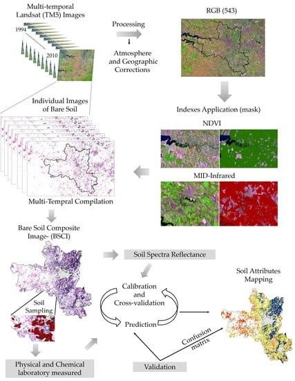
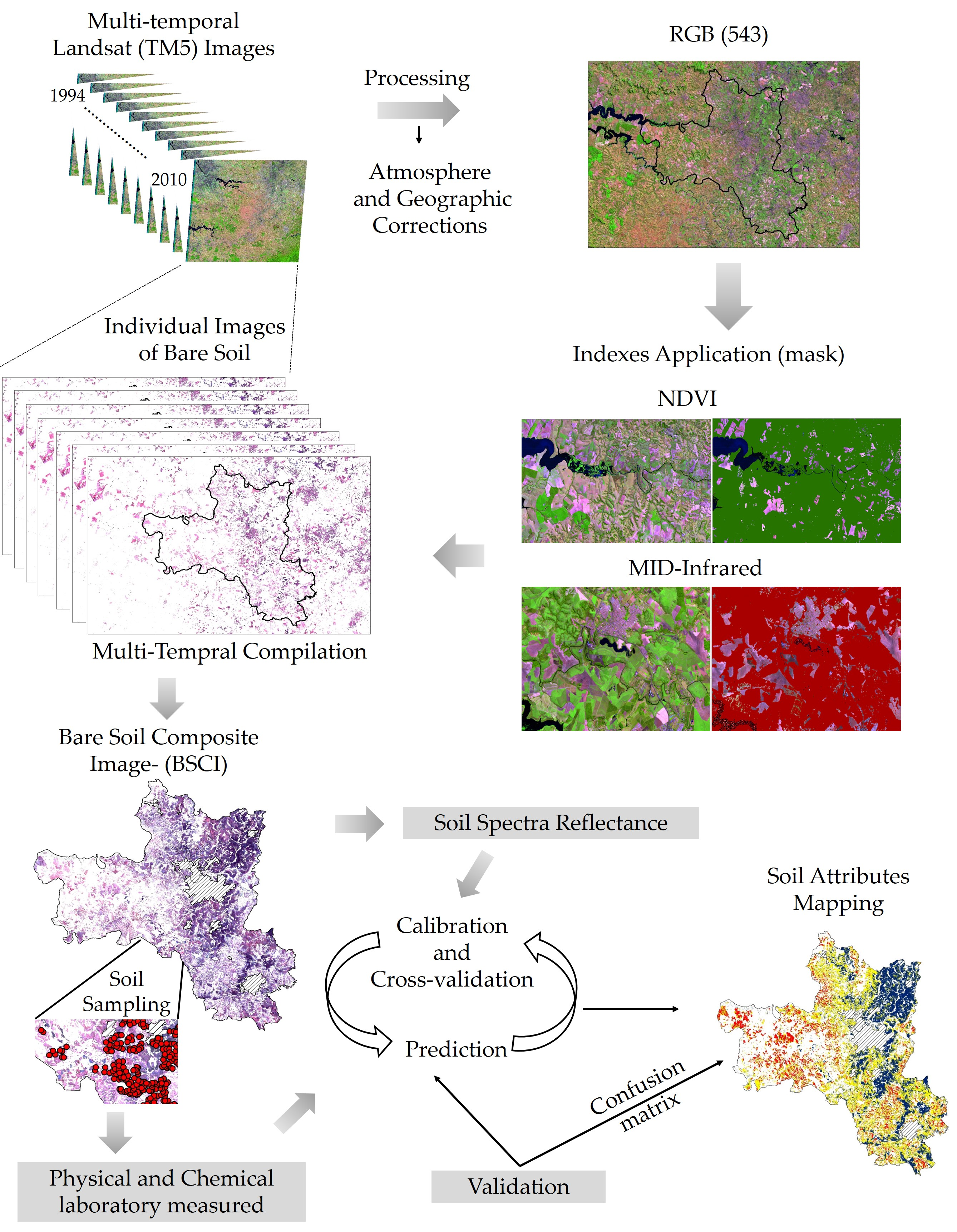
2.2. Multi-Temporal BSCI

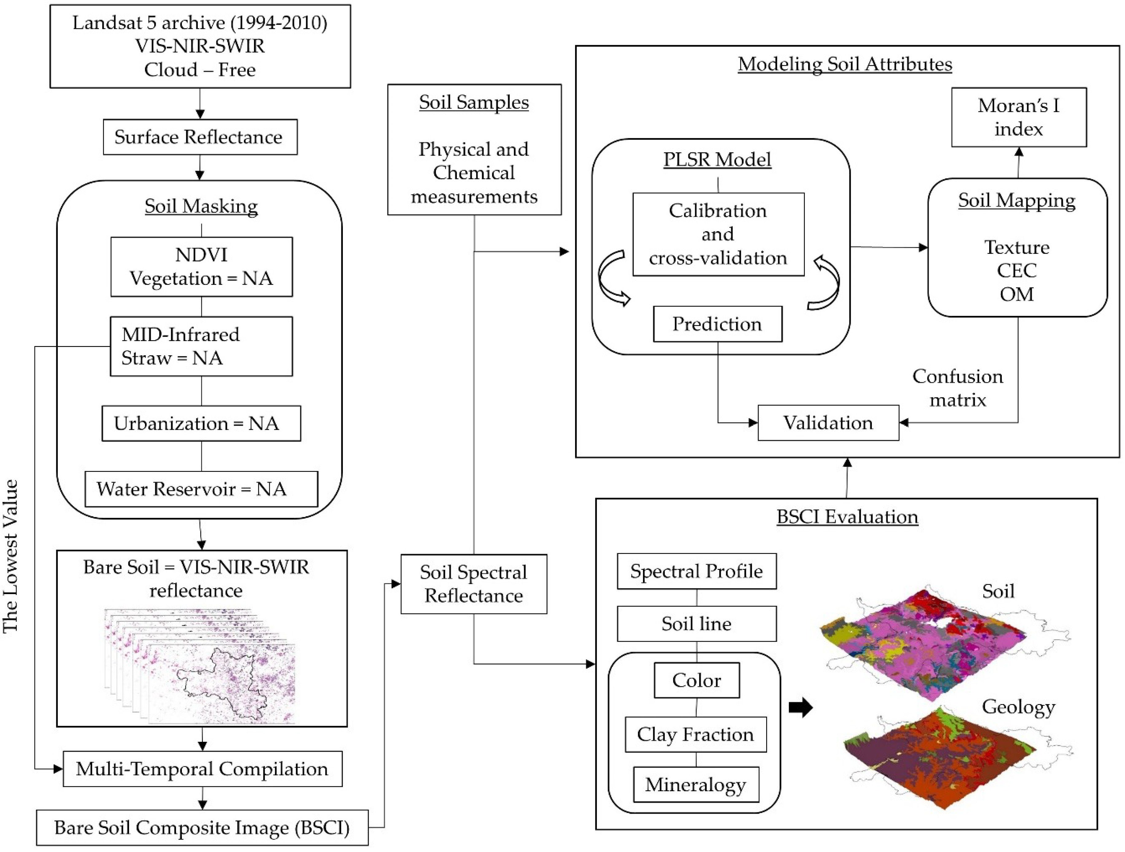
2.2.1. Image Acquisition

Thirteen cloud-free Landsat 5 TM images from the dry season (June to September) between 1994 and 2010 were selected. The dry season was chosen to reduce moisture conditions in the agricultural fields as high soil moisture content decreases soil reflectance and affects the features of the spectral profile, influencing absorption features [33].

These images acquired at 30m spatial resolution from orbit 220 and point 70 were downloaded from http://earthexplorer.usgs.gov/, at the 1-T processing level, orthorectified and with 8-bit radiometric resolution. The spectral resolution used covers an electromagnetic spectrum ranging between VIS (Band 1—TM1, Band 2—TM2, Band 3—TM3), NIR (Band 4—TM4), and SWIR (Band 5—TM5, Band 7—TM7) wavelengths.

2.2.2. Image Preprocessing

The geometric and atmospheric corrections and the spectral analysis were performed using the ENVI (Environment for Visualizing Images) program (Exelis Visual Information Solutions, Boulder, Colorado). Clipping processes, index calculation, and masks of the multispectral images were executed on the ArcGIS program [34].

The geometric corrections were performed using control points obtained in the field with GPS (Global Position System) equipment [35]; the images were then reprojected to the Universal Transverse Mercator system (UTM/Zone 23/South). The atmospheric correction was performed with the FLAASH module (Fast Line-of-sight Atmospheric Analysis of Spectral Hypercubes), which integrates the MODTRAN (Moderate Resolution Atmospheric Transmission) radiation transfer code and accounts for water vapor and aerosol retrieval [36]. This preprocessing aimed to normalize the digital data and eliminate the addictive effects of the atmosphere.

The steps of this technique, according to Chander et al. [37], consist of converting the digital numbers from pixels to radiance, for which the Radiometric Calibration tool of the ENVI program was used. Then, the conversion of the radiance to top-of-atmosphere reflectance and the top-of-atmosphere reflectance to surface reflectance were performed using the FLAASH module. The images resulted in gray level or minimum digital number (zero value) corresponding to 0% reflectance, and the highest gray level (255), through to 100% reflectance [38], thus, the reflectance data of the historical series of the satellite images could be compared to each other.

The reflectance data of the soil (texture variation), sugarcane, and straw obtained under laboratory conditions indicated regions of reflection and absorption in the spectral bands of Landsat 5. In the electromagnetic spectrum, the TM3 band captures strong absorption by green vegetation reflection, and TM4 expressively reflects the energy of vegetation targets. It indicates good contrast between pixels of vegetation and those without it (bare soil) [39]. The TM5 and TM7 bands also contrast both targets. These bands in the electromagnetic spectrum are positioned in the region of strong reflection of soils and high absorption of healthy vegetation [40] (Figure 4a). TM3 (RED), TM4 (NIR), TM5 (SWIR1) and TM7 (SWIR2) were used to compose the RGB (5, 4, 3 or 7, 4, 3) image and the spectral indices.

Estimation of soil properties, such as clay content, is hampered if vegetation or crop residues cover the pixels. These targets are often spectrally similar; however, they differ in intensity and shape of the VIS-NIR-SWIR wavelengths.

2.2.3. Soil Masking

Pixels of bare soil are required to evaluate soil properties. A model was developed in the model builder tool of the ArcGIS program to detect residue cover and green vegetation classes in each image. This model is a diagram that chains together geoprocessing tools and build automate workflows. The model was built to create a mask of bare soil, the chains of the workflows analyzed simultaneously the Normalized Difference Vegetation Index (NDVI) profile and MID-Infrared index profile over all the images, another process was to clip water reservoirs, and urban sites. The mask targets were flagged as not available values (NA) (Figure 1).

The NDVI is an index that differentiates vegetation in satellite images, evaluating the variation of a green area within a certain period. The index calculation is represented in Equation (1) [41] and varies from −1 to 1. In Figure 4a, the values below the thresholds were an input to the model creating a mask for non-vegetation patterns (i.e., bare soil or straw).

$$\mathrm{NDVI}=\frac{\mathrm{NIR}-\mathrm{R}}{\mathrm{NIR}+\mathrm{R}}$$

(1)

where, NDVI is the Normalized Difference Vegetation Index; NIR is the reflectance value on near infrared of Band 4—TM4; and R is the reflectance value on red of Band 3—TM3.

The MID-Infrared index was calculated to mask soil texture classes and straw (Figure 4a,b). Then, as described by Demattê et al. [18], bands TM5 and TM7 (near lignin band) were used to discriminate between these two objects. The MID-Infrared index (Equation (2)) is used to establish thresholds to contrast soils and straw to obtain only pixels of bare soil. Hence, values below the bottom limits were used to create the model to mask straw (Figure 4a).

$$\mathrm{MID}-\mathrm{Infrared}=\frac{\mathrm{SWIR}1-\mathrm{SWIR}2}{\mathrm{SWIR}1+\mathrm{SWIR}2}$$

(2)

where, MID-Infrared is the normalized difference between Band 5—TM5 and Band 7—TM7 index; SWIR1 is the reflectance value on near-infrared Band 5—TM5; SWIR 2 is the reflectance value on near-infrared Band 7—TM7.

2.2.4. Design of BSCI

A composite image was constructed, adapted from Dematê et al. [18], which operated an algorithm in R program language [42]. The algorithm requires the bare soil mask image and the MID-Infrared index image as input files. The lowest value of the MID-Infrared index was established to standardize the multi-temporal occurrences of bare soil for the same pixel. This algorithm selected the pixel of lowest MID-Infrared index value from all possible occurrences for a given pixel to finally create the BSCI (Figure 1).

2.2.5. Evaluation of the BSCI

From the BSCI, multi-temporal spectra data (TM bands) from the soil sample points (Figure 2) were extracted using the Extract Multi-Value by Points tool of ArcGIS program [26] for spatializing soil attributes.

The spectral profile and soil line concept [43] were applied to the multi-temporal spectra data to verify the BSCI. The soil line concept is useful for evaluation of the bare soil pixel [19]. The soil line is a two-dimensional diagram (scatterplot) that contrasts the reflectance values obtained from TM3 and TM4 bands, which starts between the X-axis and the Y axis at 45 degree inclination. It presents linear correlation (1:1), and the bare soil pixels must be located close to the 1:1 line.

A comparison between the BSCI, the conventional soil and geology map [25,26] (Figure 3) was carried out. The Tukey’s test for mean comparison of reflectance according to each geology classes was used when p < 0.05. The area was divided into six subsites to make comparisons related to the mineralogy of the soils, the composition of the clay fraction and the color of the satellite images. These were the only maps available for the area, besides the scale map and the spatial resolution that did not match with the satellite resolution.

2.3. Soil Attribute Modeling

The partial least square regression (PLSR) was used to calibrate soil attribute (clay, sand, CEC, soil organic matter (SOM)) models using Unscramble software [44]. For each soil attribute, the model calibration divided the multi-temporal spectra data of BSCI into calibration and validation sets, of which 80% of the spectra were used in calibration, while the remaining 20% were employed for validation. The models were evaluated based on the coefficient of determination (R²), root mean square error (RMSE) and the ratio of performance to deviation (RPD) for both calibration and validation datasets [45].

The prediction models of soil attributes were applied to the Bare Soil Composite TM bands using R program language [42]. Additionally, the predicted clay content map was classified as clay (>600 g kg⁻¹), clay-loam (350–600 g kg⁻¹), loam (150–350 g kg⁻¹) and sand (<150 g kg⁻¹) [28]. The OM (g kg⁻¹) was classified as low (<10), medium (11–15), high (16–25) and very high (>25) content. The CEC (mmol_c kg⁻¹) was categorized into low (>30), medium (31–60), high (61–80), and very high (>80) content. Moran’s I spatial autocorrelation index was applied to evaluate the spatial distribution of the measured soil attributes and to assess whether each soil attribute presents random, dispersed, or clustered pattern [46]. For this, a grid point of the map attributes was created, and Moran’s I index was performed using the ArcGIS program [34].

A confusion matrix was also used to validate the predicted maps by comparing the measured class from the validation points (20%) and the respective predicted class. Overall accuracy, the Kappa coefficient [47], and the user’s accuracy and the producer’s accuracy were calculated. The overall accuracy is the ratio between the sum of all pixels correctly classified and the total number of validation pixels. The Kappa coefficient indicates the level of agreement between measured and predicted observations. This coefficient is used to account for the possibility of data being correctly clustered by chance [48] (Equation (3)).

$$K=\frac{{\theta }_1-{\theta }_2}{1-{\theta }_2}$$

(3)

where, K is the Kappa coefficient; θ₁ is the weighted observed agreement; and θ₂ is the weighted chance agreement.

Components located on the diagonal of the confusion matrix have the maximum weight on a linear scale. Components further from the correct ones receive lower weights. The level of agreement classification by Landis and Koch [49] was considered to evaluate map quality. Kappa values from 0.21 to 0.40 are considered as fair agreement; from 0.41 to 0.60, moderate agreement; from 0.61 to 0.80, substantial agreement and values above 0.81, almost perfect agreement.

3. Results and Discussion

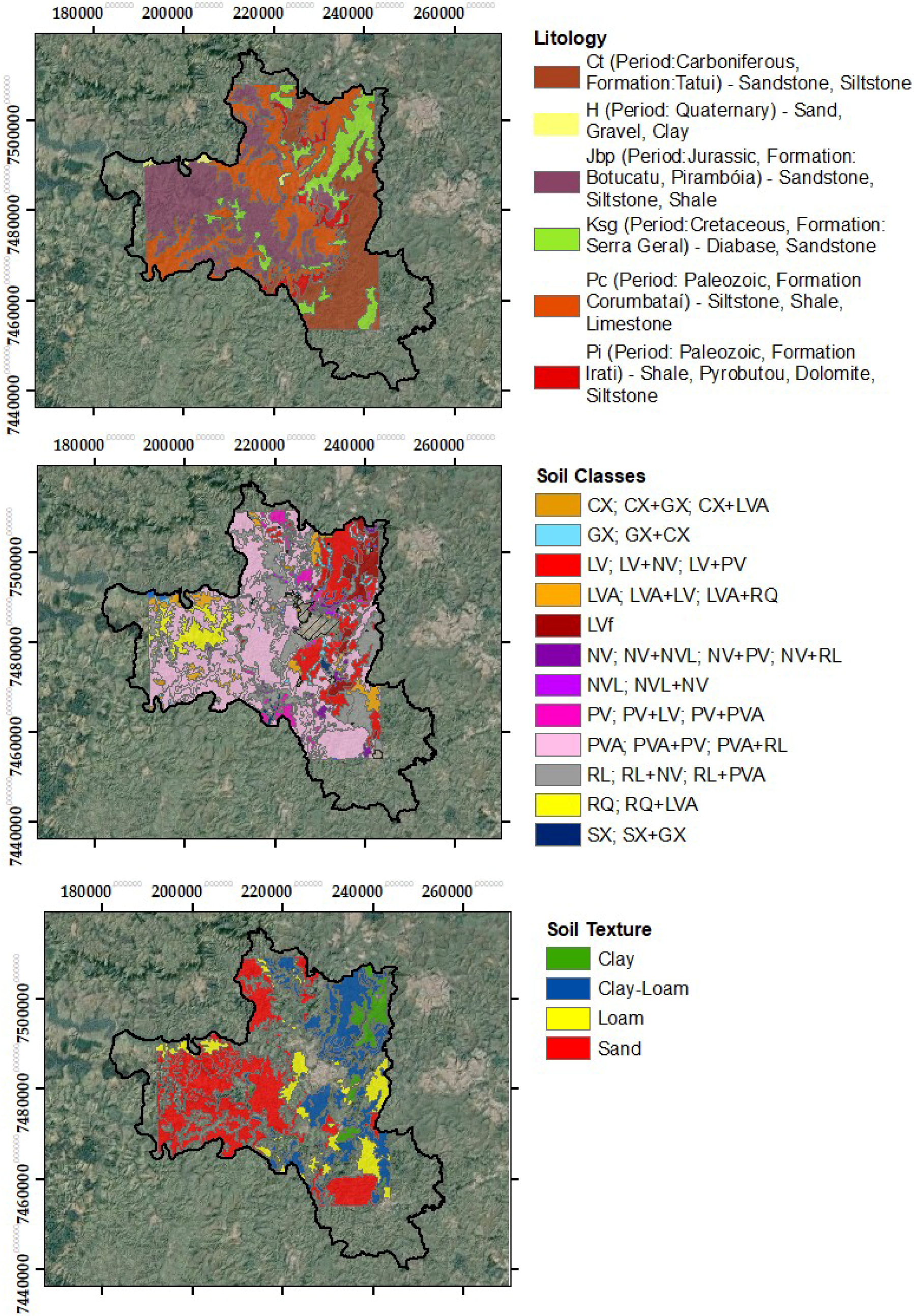
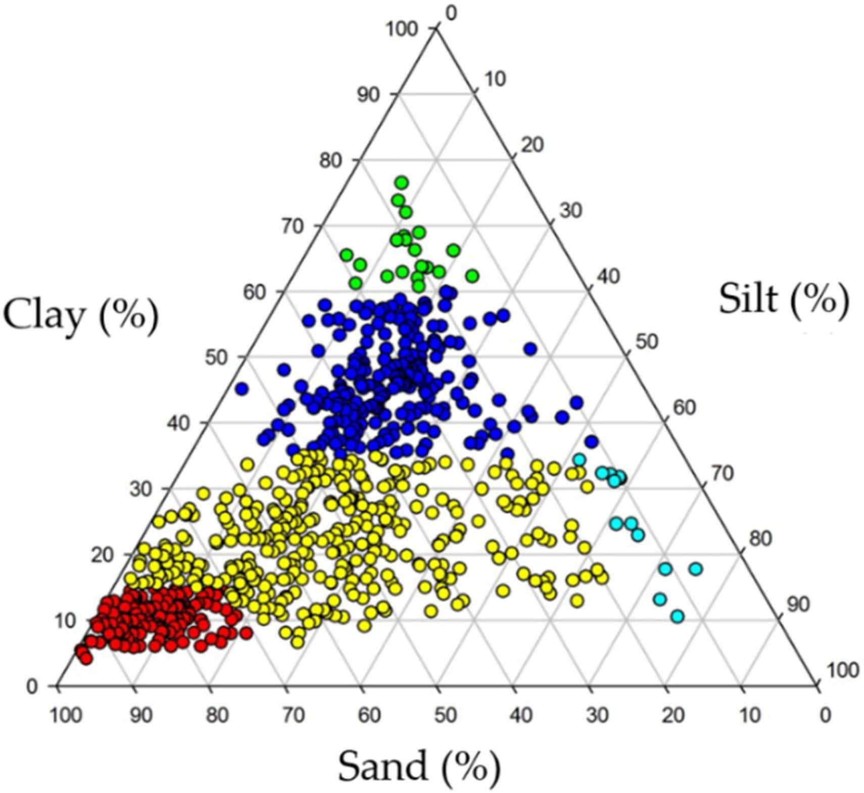
3.1. Soil Characterization

The soil property (0–20 cm) summary statistics indicate high variability of all physical and chemical soil attributes (

Table 2. Summary statistics of laboratory determined soil attribute measurements.

Soil Attribute	Minimum	Maximum	Mean	SD 1	CV 2
Sand (g kg−1)	70.0	940.0	507.5	220.0	43.4
Silt (g kg−1)	4.0	765.0	212.7	140.4	66.0
Clay (g kg−1)	41.0	765.0	279.7	158.8	56.8
SOM 3 (g kg−1)	0.0	52.0	17.7	8.4	47.7
P (mg kg−1)	1.0	373.0	19.2	33.2	172.8
K+ (mmolc kg−1)	0.0	72.0	2.7	5.5	203.3
Ca2+ (mmolc kg−1)	2.0	356.0	35.6	34.8	97.6
Mg2+ (mmolc kg−1)	1.0	108.0	13.6	11.9	87.5
Al3+ (mmolc kg−1)	0.0	38.0	2.4	3.9	160.4
H+ (mmolc kg−1)	1.0	296.8	33.1	20.8	62.9
SB 4 (mmolc kg−1)	3.0	461.9	52.3	46.1	88.1
CEC 5 (mmolc kg−1)	14.6	481.9	85.4	49.1	57.5
V 6 (%)	9.0	96.9	57.3	19.7	34.4
m 7 (%)	0.0	62.0	6.6	10.7	162.0

¹ Standard deviation; ² Coefficient of variation; ³ Soil organic matter; ⁴ Sum of bases; ⁵ Cation exchange capacity; ⁶ Base saturation; ⁷ Aluminum saturation.

). The chemical attributes have a higher variability than the physical attributes, although their status is suitable for plant development. Croplands are the most common land use of the region. Common soil textures are sand, loam, and clay-loam (Figure 5). Clay content, for instance, is between 41 and 765 g kg⁻¹, with a variation of 70% (Table 2). SOM presents values between 0 and 52 g kg⁻¹, varying by 50%. The amplitude of values for SOM is related to tropical conditions, which are highly affected by environmental factors and especially by soil management practices, which impacts the steady state over time [50]. The clay, silt and sand contents are less impacted by agricultural practices when compared to the chemical properties and SOM. However, the high variability presented in Figure 5 shows the influence of the complex geology of the region.

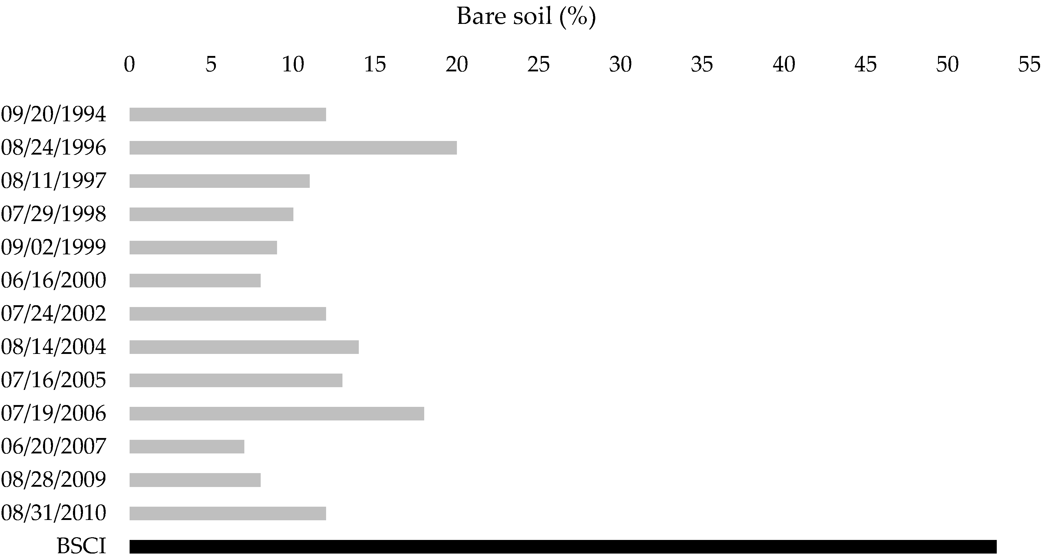
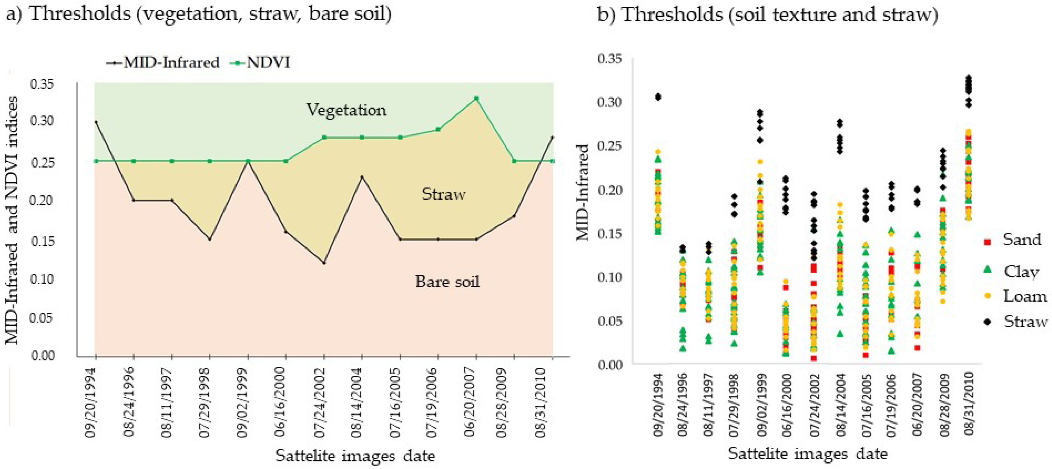
3.2. Multi-Temporal Bare Soil Detection

The percentage of bare soil for each of the 13 images varied from 7% (20 June 2007) to 20% (24 August 1996) (Figure 6), with an average bare soil coverage of 12% in the area. Many pixels of bare soil occur in the same croplands, indicating that with time the bare soil occurrences overlap. In fact, in only a few images, it was observed that there were moments in time when the increase in bare soil is higher than the average. The selection period covered the months of July and August, which corresponds to the dry season, often coinciding with the practice of plowing management. The availability of satellite images in the dry season is limited but efficient. Thus, it is possible to detect large areas of bare soil in the dry season. Moreover, images are often influenced by clouds during the rainy period and are consequently not suitable for analysis.

Some pixels had no bare soil at any time, which were classified as NA. These NAs correspond to land uses such as urban areas (6% of the area), water bodies, forests, perennial crops, and grassland (41% of the area). Thus, it will be difficult to reach 100% bare soil for this study site. The BSCI presented 53% (128,260 ha) of bare soil coverage (Figure 6). The BSCI is defined as an almost continuous soil surface constructed from 16 years of 30 m spatial resolution Landsat images, representing the spectral surface variability of soils for the agricultural area of Piracicaba. The results demonstrated that the temporal coverage of bare soil is dependent on Landsat coverage, weather conditions and land management system according to crop type.

3.3. BSCI

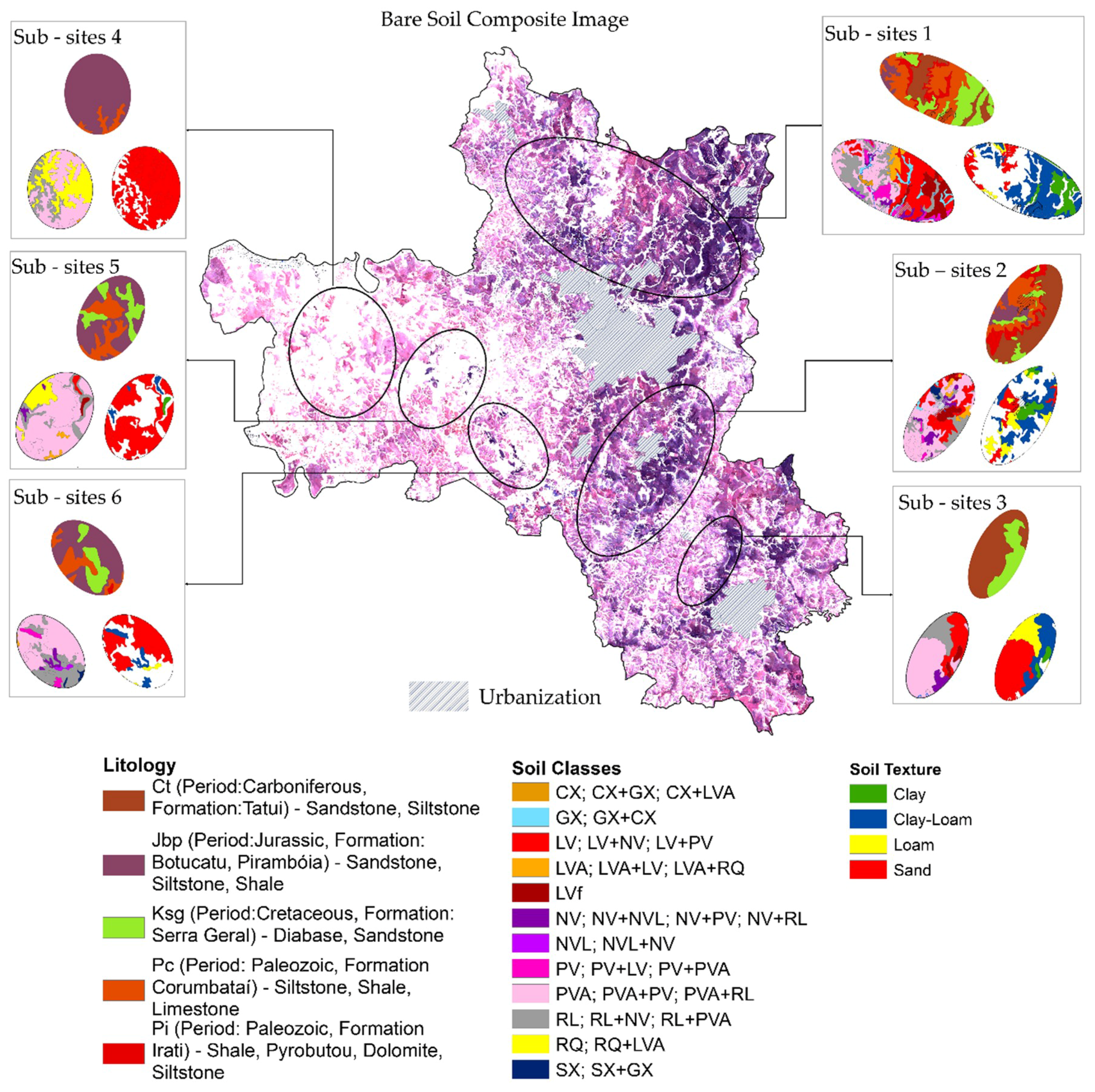
3.3.1. Bare Soil Composite Image Related to Soil and Geology

The BSCI shows more bare soil in subsites 1, 2 and 3 (Figure 7), which are related to areas with sugarcane crops. However, the BSCI in sub-areas 4, 5 and 6 illustrates very steep sites with less bare soils, upon which mechanization is hindered, leading to a prevalence of grassland and perennial crops, where the soil is rarely exposed by plowing.

The degree of soil evolution and weathering intensity determines the mineralogical composition of the clay fraction, which is essential for evaluating the soil spectral profile [51]. Tropical soils may have different proportions of oxides in their mineralogy, causing color variations and consequently influencing the spectral reflectance retrieved from satellite images [19]. Soils derived from volcanic rocks and with high iron content have a lower reflectance intensity (high absorption), while soils with medium to low iron content have intermediate and high values of reflectance intensity (low absorption) [52].

The variations in the BSCI are represented by the false color composition (R-TM5, G-TM4, B-TM3) (Figure 7), and are mostly related to clay proportions, soil color, and mineralogy (e.g., oxides, kaolinite, and quartz). The RGB values vary from 0 to 255, whereby low values (low reflectance) generate darker colors that indicate higher amounts of clay and oxides. Lighter shades indicate sandy soils, which have higher reflectance due to lower clay and iron oxide content. Clearly, the BSCI variations represented by false color compositions are extremely important because they enable quick assessment of soil texture and mineral distribution across the study site.

The legacy geological and soil type maps were important in the establishment of relevant relationships between parent material, soil types, and image reflectance data. The mean reflectance of all bands is statistically different according to geology classes in accordance with the Tukey test at p < 0.05 significance (

Table 3. Mean reflectance variation according to geology classes.

Geology	B1		B2		B3		B4		B5		B7
Jbp	7.48 ± 2.93	A	10.25 ± 2.99	A	14.27 ± 3.51	A	22.42 ± 5.33	A	34.36 ± 9.05	A	29.32 ± 7.41	A
Ct	6.35 ± 3.18	B	9.27 ± 3.45	B	13.1 ± 3.88	B	19.85 ± 5.75	B	28.18 ± 8.59	B	23.68 ± 7.02	B
Pc	6.28 ± 2.84	C	8.85 ± 2.91	C	12.59 ± 3.26	C	19.33 ± 5.00	C	27.7 ± 8.16	C	23.49 ± 6.73	C
Pi	4.82 ± 2.39	D	7.34 ± 2.36	D	10.97 ± 2.68	D	16.58 ± 3.95	D	23.75 ± 6.59	D	19.94 ± 4.85	D
Ksg	4.15 ± 2.45	E	6.56 ± 2.57	E	10.11 ± 2.98	E	15.21 ± 4.58	E	20.54 ± 7.45	E	17.19 ± 5.70	E

Means followed by similar capital letters in the same column does not indicate differences between geology classes accordingly Tukey test (p < 0.05).

). This demonstrates that the BSCI correctly detects variations in soils, which are related to the parent material.

The qualitative comparison covered 80% of the study site [25,26] (Figure 3). The proportion of soil surface texture variation was 33% for sandy, 18% for clay-loam, 9% for loamy, and 4% for clay soils, although 34% were not classified (Figure 3c). Locations discriminated as “no classification” correspond to areas not covered by the legacy soil map (semi-detail scale). These sites refer to Lixisol (PV) and less representative soil classes, including Planosol, Gleysol, and Cambisol (SX, GX, and CX). These patterns are not frequent on the legacy map but appear with more frequency as the number of field observations increases. In this case, the BSCI could achieve greater detail from the soil surface as it has 30 m spatial resolution, which is more detailed than the legacy soil maps.

The BSCI correctly detects small scale variations in soil texture, as in subsites 5 and 6 (Figure 7), where small abrupt changes of clay-loamy and clayey soils can be observed in a predominantly sandy texture location. Moreover, the BSCI detected the neo-Cenozoic sites located in the highest parts of the landscape. These sites correspond to subsite 1, 2 and 3, in stains of diabase, where occurrences of Ferrolsol and Nitosol (LV/LVf/NV/NVL) are described. These spots are detected as clayey and clay-loamy texture by the BSCI. Thus, the BSCI variation in texture for these soils matches the legacy maps.

Despite the low scale of the lithology map (1:100.000), the Botucatu and Pirambóia Formations (Jbp) are associated with Arenosol (RQ) (subsite 4—Figure 7), and they are sandy texture throughout the soil profile. The sandy texture detected by the satellite image enables the inference that they are Arenosol (RQ). Nevertheless, Lixisol (PV) may be sandy/loamy at the surface and loamy/clay-loamy or clayey in subsurface layers; but the image does not detect the B-horizon, thus confusing PV with RQ.

These results show that BSCI is an effective tool that can provide support to new soil surveys and update legacy maps. Furthermore, it may be used to extrapolate or interpolate areas with no available information on soil attributes. Considering that satellite images may be limited in the discrimination of some soil classes, such information may be combined with relief data when mapping soil types [53] (e.g., slope, curvature, topographic index). In addition, the relief could improve the detection of sites where Planosol, Gleysol, and Cambisol (SX, GX, and CX) appear, especially when related to drainage features.

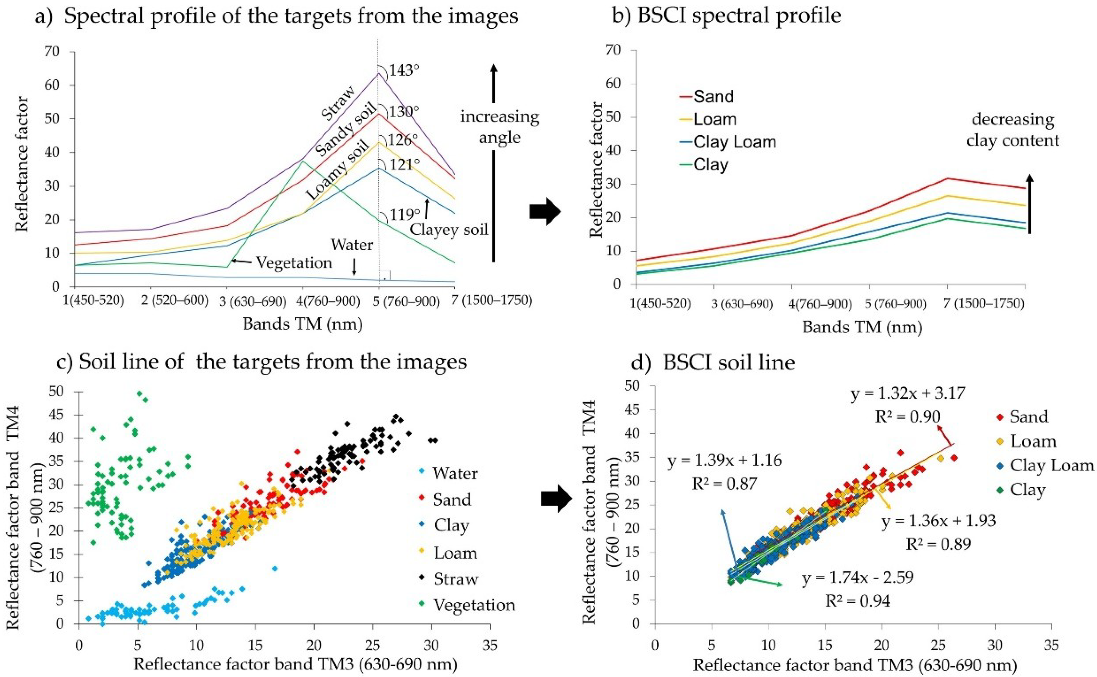
3.3.2. Evaluation of Spectral Data (Spectral Profile and Soil Line)

The soil spectra were obtained from the Landsat image of each sampling location (Figure 8a). A great concern when using satellite images is the influence of soil moisture and surface roughness (shadow) in the spectral profile [22,54]. The spectral features are more affected by soil moisture, which is related to the water absorption bands around 1800 and 2119 nm (SWIR range) [55]. Clayey soils with significant amounts of SOM have higher water holding capacity than sandy soils, thus soil moisture has a positive correlation with clay content and SOM, and, consequently, a negative correlation with soil sand content [22]. To reduce the influence of external factors, atmospheric correction and data transformation to reflectance were performed. In addition, images from the dry season were selected and their quality with MID-Infrared index assessed, before calculating the BSCI [33]. Meanwhile, the profile demonstrates intensity and form of the soil spectral data. The intensity of BSCI spectra increases from Band 1 to Band 5. Besides that, sandy soils present higher reflectance and ascending shape when compared to clay-loamy soils (Figure 8b).

Among the spectral features influenced by quartz, there is an angular variation in TM5 [19,54]. Soils with loamy or clayey texture have lower angles in comparison to sandy soils, which agrees with the findings of Madeira, Netto and Baptista [56]. Pixels corresponding to vegetated areas may be clearly differentiated from other targets by the angle of 119° and by their high reflectance in band TM4 (NIR). The low spectral reflectance of water, which absorbs energy in the entire electromagnetic spectrum, is characterized by an angle of 90°.

The spectral behavior of areas covered with crop residues in the satellite images has a shape and intensity similar to those shown by sandy soils, which cause misunderstanding. However, two aspects differentiate straw from sandy soil: (1) straw presents higher reflectance intensity, and (2) the angular difference of TM5 is greater for straw than for sandy soils. Therefore, through the MID-Infrared index, it is possible to differentiate satellite images with an exposition of straw from those with bare sandy soils.

Here, the MID-Infrared index threshold was defined based on interpretation of the images (Figure 4a,b) and related to field observation analysis and Landsat images. Thus, this index is efficient for a drier period with sufficient land cover. This work brings the novelty of using a threshold for each image, instead of a mean value for all images. It increases the sensibility of the procedure, providing a realistic representation of bare soil conditions.

The spectral profile (Figure 8b) confirms that the BSCI only corresponds to bare soil, as it presents similar shape and intensity compared to the satellite multispectral data of Demattê et al. [19]. Besides the granulometric properties, iron content is also responsible for variations in satellite TM5 reflectance [19,54]. Clayey and clay-loamy soils that present high hematite (iron oxide) content have lower reflectance intensity with a horizontal curve. This is an evident feature among samples from the same parent material, as in the case of soils derived from diabase, such as in the Ferralsol (LV/LVf) and Nitosol (NV/NVL). Yet, as the iron content decreases the soil reflectance increases, as in the Ferralsol (LVA) and Lixisol (PV/PVA). Furthermore, in these soils, the hematite decreases, and the goethite increases. Therefore, as the sandy texture becomes more pronounced (e.g., in the Arenosol-RQ), higher reflectance is observed, with an even higher peak in TM5.

The soil line plot from bands TM3 and TM4 (red and NIR wavelengths) (Figure 8c) is useful to understand surface variations and identify bare soil areas [35,36]. Such a method is employed to discriminate different soil types based on texture, iron content and organic matter variations [19,54]. Bare soil occurs in regions where the albedo approaches the 1:1 line of the plot, but in sandy soils, the reflectance spreads (Figure 8c). The low reflectance values in red (TM3) and high values in NIR (TM4) are found in pixels with higher proportions of vegetation. In the bottom left portion of the scatter plot are the pixels corresponding to water reservoirs (Figure 8c).

The soil line of the BSCI was found by calculating the intercept of lines, slope, and coefficient of determination (R²), which change according to variations in bare soil reflectance [42] (Figure 8d). The statistics of the BSCI soil line show high R², which confirms BSCI pixels as being bare soils. The reflectance variation of soil texture was adjusted by different soil lines. Similar parameters were observed, but with slight changes from clay-loamy to loamy soils. Additionally, each soil texture class had a slope shift from the 1:1 line. The slope coefficient and intercepts varied with reflectance, whereby clayey soils had lower intensity (Ferralson—LVf), presenting negative intercept values and higher slope coefficient values, which agrees with Demattê and Terra [54]. Clayey soils (19 observations) and clay-loamy soils (218 observations) on the soil line plot (Figure 8c) correspond to ferric oxide soils according to Demattê et al. [19]. Thus, Ferrasols and Nitossols (LVf/LV/NV/NVL) are positioned near the origin of the soil line. The loamy soil albedo (295 observations) and sandy soils (203 observations) tend to be positioned further from the origin of the soil line plot. In our study, these texture classes correspond to Lixisols (PV) and Arenosols (RQ), respectively, and agree with the findings of Demattê et al. [19].

3.4. Soil Attribute Modeling

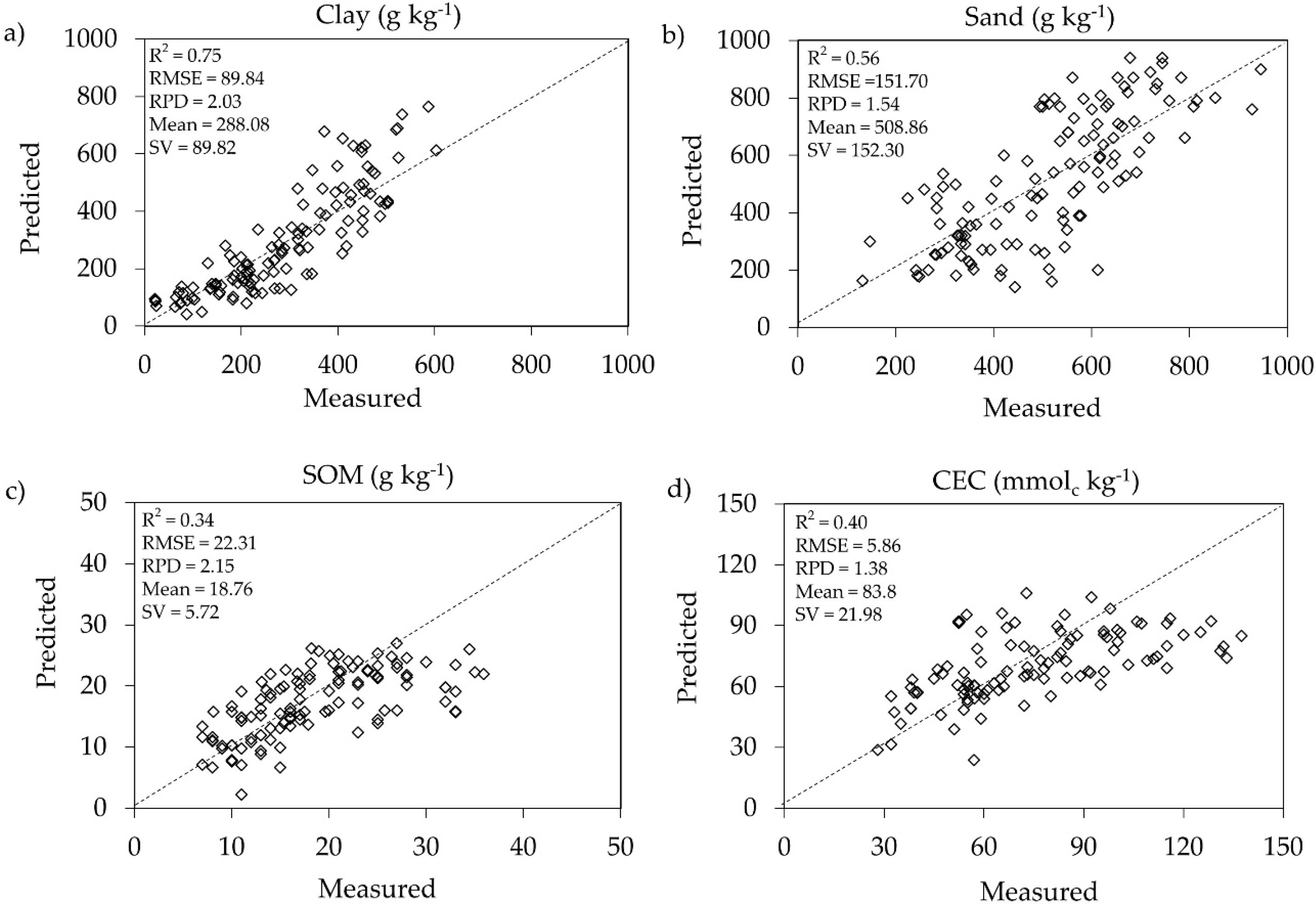
3.4.1. Calibration and Validation

Soil attribute prediction of the cross-validation of the validation dataset is shown by the coefficient of determination (R²), root mean square error (RMSE) and the ratio of performance to deviation (RPD) for sand, clay, CEC and soil organic matter (SOM) (Figure 9). SOM presented the lowest error among the soil attributes. RPD presents good prediction accuracy, according to Chang et al. [57], as it is in the interval between 1.5 and 2.0. Dunn et al. [58] propose that models with RPD greater than 2.0 are excellent; therefore, the clay content and CEC models are both stable and excellent in their prediction accuracy. According to Viscarra Rossel et al. [59], the RPD values for clay and CEC models are considered good and very good. RPD values equal to 1.4 and 1.5 for the SOM and sand content models are considered fair and may be useful for mapping purposes.

Predicted versus measured values for the soil attributes are presented in (Figure 9). For clay and sand, the range of the predicted values is similar to the measured values. CEC and SOM estimates had a slightly narrower range compared to the measured values, indicating underestimation for these attributes. We noted similar mean values in the summary statistics from the measured (Table 2) and validation predicted dataset values (Figure 9). The standard deviation of the predicted value is smaller, especially for SOM and CEC, meaning that the extreme values are not well represented.

Considering the distance of 800 km from the Earth’s surface to the satellite sensor, as well as the spatial resolution of 30 m, the predictions present satisfactory performance. Furthermore, this method is fast and suitable for several temporal and spatial scales. The tendency is increasing demand for regional and global methods to obtain soil information [9]. The reason for such increasing demand is related to ecosystem services and global land monitoring, aiming to reduce soil loss and degradation [60]. The method presented in the present study has the potential to quantify soil attributes, providing spatially explicit information over extended areas. Other similar studies, based only on Landsat data, have also shown positive results in their predictions of soil attributes [20,21,22,23]. Therefore, digital soil mapping integrated with other geotechnologies has the potential to aid soil surveys.

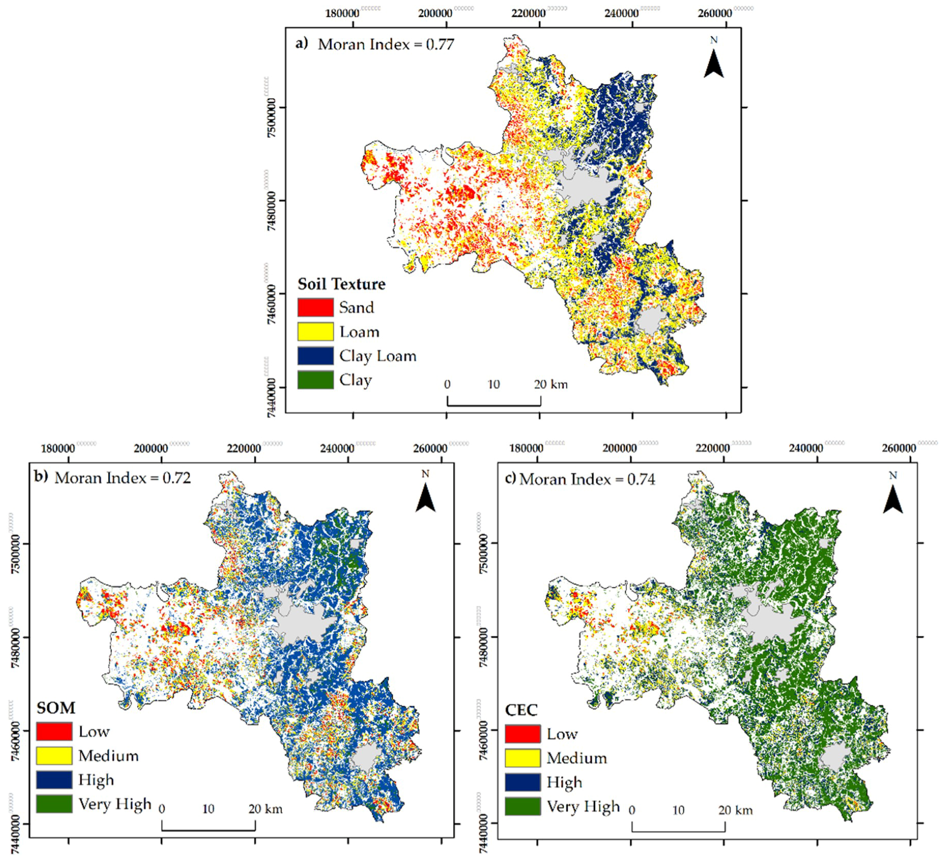
3.4.2. Soil Attribute Mapping and Autocorrelation Analysis

The results of the PLSR for clay content, CEC and SOM (Figure 10) showed a similar pattern that matches well with the geology and soil type of the study site (as described in Section 2.1 and Section 3.3.1). Furthermore, the high Moran index demonstrated that spatial distribution of the predicted attributes is clustered.

Sand content is almost inversely related to clay content, thus only the soil texture map based on clay content is presented (Figure 10a). In tropical soils, where weathering is very intense, the occurrence of silt is very low (Figure 5). Thus, the majority of granulometric particles are constituted of sand and clay. Predicted clay varied from 3 to 797 g kg⁻¹ (Figure 10a). Loamy soils accounted for 47% of the classified pixels, followed by 33% for clay-loamy soil and 18% for sandy soil; the remaining were those of clayey soil. Textural classes varying from clay-loamy to clayey are related to areas of intensive cultivation. As expected, in these areas the CEC was classified as very high, with values above 80 mmol_c kg⁻¹.

Predicted SOM content varied from 0 to 32 g kg⁻¹ and predicted CEC varied from 0 to 140 mmol_c kg⁻¹. Among the distribution of organic matter content pixels, 65% included the medium class of SOM and approximately 5% of the pixels represent very high class.

In loamy, clay-loamy, and clayey soil areas, very high class CEC predominated, representing 70% of the pixels. In areas with sandy soils, the mean values of medium class CEC predominated, which represents 21% of the pixels, while less than 1% have values below 30 mmol_c kg⁻¹. In these areas, around 10% of the pixels presented values lower than 10 g kg⁻¹ of SOM, mostly represented by Arenosol (RQ). These low SOM contents are related to the rapid decomposition of organic matter content in sandy soils.

Clay content is related to intrinsic factors of formation, such as parent material. However, CEC and SOM are related to extrinsic factors, which can be influenced by the type of land management. As such, defining textural classes is advantageous, as they do not vary with anthropic factors and may assist in defining homogeneous soils. Furthermore, to capture variability of CEC and SOM over time, application of PLSR models to each moment in time is suggested, as implemented by Diek et al. [22]. Despite the detected influence of soil moisture over the season, this technique may be efficient in monitoring soil attributes over time.

The additional validation of maps is presented in the confusion matrix, where 123 points were used (

Table 4. Confusion matrix tables between measured versus predicted soil attributes.

Soil Texture		Measured				Total	Producer Accuracy (Precision) (%)
		Sand	Loam	Clay-Loam	Clay
Digital Soil Texture Map (Predicted)	Sand	1	10	0	0	11	9.1
	Loam	0	26	2	0	28	92.86
	Clay-Loam	5	0	40	1	46	86.96
	Clay	0	0	14	24	38	63.16
Total		6	36	56	25	123
User Accuracy (%)		16.67	72.22	71.43	96.00
Overall Accuracy = 73.98%, Kappa = 0.63
SOM 1 Class		Measured				Total	Producer Accuracy (Precision) (%)
		Low	Medium	High	Very High
Digital SOM Map (Predicted)	Low	9	7	3	0	19	47.37
	Medium	8	12	9	0	29	41.38
	High	1	8	33	2	44	75.00
	Very High	1	4	24	2	31	6.45
Total		19	31	69	4	123
User Accuracy (%)		47.37	38.71	47.83	50.00
Overall Accuracy = 45.53%, Kappa = 0.23
CEC 2 Class		Measured				Total	Producer Accuracy (Precision) (%)
		Low	Medium	High	Very High
Digital CEC Map (Predicted)	Low	1	1	2	1	5	20.00
	Medium	1	22	13	5	41	53.66
	High	0	5	14	5	24	58.33
	Very High	0	3	23	27	53	50.94
Total		2	31	52	38	123
User Accuracy (%)		50.00	70.97	26.92	71.05
Overall Accuracy = 52.03%, Kappa = 0.31

¹ Soil organic matter. ² Cation exchange capacity.

). From these results, producer accuracy (precision) and user accuracy of the soil attribute maps, and consequently the Kappa coefficient (K) were determined. The overall accuracy of soil texture mapping represents 74% (Kappa = 0.63), which is considered very good [49]. Loamy and clay-loamy soils respectively presented higher producer accuracy at 93% and 87%, demonstrating that the classification probability agrees with the field validation measurements. Concerning the user accuracy, almost all classes demonstrated high probability, with loam, clay-loam and clay having a chance of being correctly predicted in 72%, 71% and 96% of the evaluated cases. Only the sand class presented low value of user accuracy due to confusion with the loam class, which could be related to loss of absorption features in the spectra.

The overall accuracy of the mapping shows 46% (Kappa = 0.23) and 52% (Kappa = 031), for SOM and CEC respectively, which is considered fair [47], whereas the high class of SOM shows 75% producer accuracy, which presented less confusion and fewer errors, being more precise when compared to other classes. The other observed classes had low values of producer accuracy, indicating a low amount of measured soil samples erroneously included in these classes. All SOM classes presented an average probability of 45%, which represents the SOM as in the measured field soil sample.

The CEC class presented over 50% precision for the medium, high, and very high classes. However, the high class presented lower user accuracy, which was caused by the high confusion with very high class. Medium and very high CEC classes demonstrated a probability of 71% for user accuracy. Digital soil attribute maps derived from the combination of multi-temporal soil spectra and PLSR models demonstrated reliable agreement for texture and moderate agreement for SOM and CEC.

4. Conclusions

The multi-temporal images provide historical and temporal information for a given area, enabling reconstruction and creation of a single composite image of bare soil. The BSCI can determine up to seven times more information than a single image from a single year. Without the system, the user would have about 7% bare soil coverage for the area, which increased to 53% bare soil when applying the technique presented in this study.

The NDVI and MID-Infrared indices are efficient in retrieving bare soil occurrences. The method is quick and capable of separating bare soil from straw, and vegetation.

The spectral data, despite the 800 km distance from the target, were efficient in determining soil attributes such as clay (R² over 0.75). Even though sand, OM and CEC presented lower values, their estimates are still significant. All digital soil maps presented high spatial autocorrelation, indicating the importance of RS products for spatial modeling.

Satellite images of bare topsoil detect variations in soils texture, which is related to parent material that is statistically significant. Soils with equal clay content on the surface and in the subsurface (Ferralsols) could be detected, but if the soil has a textural gradient (i.e., Lixisol), this technique is limited.

The use of a product with 30 m resolution, which represented 242,000 ha with an almost continuous bare soil surface, opens possibilities in several areas such as land use planning, environmental monitoring, attribute mapping, precision agriculture, digital soil mapping, and updating legacy surveys.

References

1. FAO. Agricultural Demand Towards to 2050 Production Response; FAO: Rome, Italy, 2013. [Google Scholar]
2. Lal, R. Soil erosion and the global carbon budget. Environ. Int. 2003, 29, 437–450. [Google Scholar] [CrossRef] [Green Version]
3. McBratney, A.; Field, D.J.; Koch, A. The dimensions of soil security. Geoderma 2014, 213, 203–213. [Google Scholar] [CrossRef]
4. Kang, B.T.; Moormann, F.R. Effect of some biological factors on soil variability in the tropics. I. Effect of precleaning vegetation. Plant Soil 1977, 47, 441–449. [Google Scholar] [CrossRef]
5. Perrier, E.R.; Wilding, L.P. An evaluation of computational methods of field uniformity studies. Adv. Agron. 1986, 39, 265–312. [Google Scholar]
6. Miller, M.P.; Singer, M.J.; Nielsen, D.R. Spatial variability of wheat yield and soil properties on complex hills. Soil Sci. Soc. Am. J. 1988, 52, 1133–1141. [Google Scholar] [CrossRef]
7. Mulla, D.J.; Bhatti, A.U.; Kunkel, R. Methods for removing spatial variability from field research trials. Adv. Soil Sci. 1990, 13, 201–213. [Google Scholar]
8. Rossel, R.A.V.; Bouma, J. Soil sensing: A new paradigm for agriculture. Agric. Syst. 2016, 148, 71–74. [Google Scholar] [CrossRef]
9. Mulder, V.L.; de Bruin, S.; Schaepman, M.E.; Mayr, T.R. The use of remote sensing in soil and terrain mapping—A review. Geoderma 2011, 162, 1–19. [Google Scholar] [CrossRef]
10. Ben Dor, E.; Taylor, R.G.; Hill, J.; Demattê, J.A.M.; Whiting, M.L.; Chabrillat, S.; Sommer, S.; Donald, L.S. Imaging spectrometry for soil applications. Adv. Agron. 2008, 97, 321–392. [Google Scholar]
11. Woodcock, C.E.; Allen, R.; Anderson, M.; Belward, A.; Bindschadler, R.; Cohen, W.B.; Gao, F.; Goward, S.N.; Helder, D.; Helmer, E.; et al. Free access to Landsat imagery. Science 2008, 320. [Google Scholar] [CrossRef] [PubMed]
12. Arrouays, D.; Lagacherie, P.; Hartemink, A.E. Digital soil mapping across the globe. Geoderma Reg. 2017, 9, 1–4. [Google Scholar] [CrossRef]
13. Ying, Q.; Hansen, M.C.; Potapov, P.V.; Tyukavina, A.; Wang, L.; Stehman, S.V.; Moore, R.; Hancher, M. Global bare ground gain from 2000 to 2012 using Landsat imagery. Remote Sens. Environ. 2017, 194, 161–176. [Google Scholar] [CrossRef]
14. White, J.C.; Wulder, M.A.; Hobart, G.W.; Luther, J.E.; Hermosilla, T.; Griffiths, P.; Coops, N.C.; Hall, R.J.; Hostert, P.; Dyk, A.; Guindon, L. Pixel-based image compositing for large-area dense time series applications and science. Can. J. Remote. Sens. 2014, 40, 192–212. [Google Scholar] [CrossRef]
15. Hermosilla, T.; Wulder, M.A.; White, J.C.; Coops, N.C.; Hobart, G.W. An integrated Landsat time series protocol for change detection and generation of annual gap-free surface reflectance composites. Remote Sens. Environ. 2015, 158, 220–234. [Google Scholar] [CrossRef]
16. Grunwald, S. Multi-criteria characterization of recent digital soil mapping and modeling approaches. Geoderma 2009, 152, 195–207. [Google Scholar] [CrossRef]
17. Samuel-Rosa, A.; Heuvelink, G.B.M.; Vasques, G.M.; Anjos, L.H.C. Do more detailed environmental covariates deliver more accurate soil maps? Geoderma 2015, 243–244, 214–227. [Google Scholar] [CrossRef]
18. Demattê, J.A.M.; Fongaro, C.T.; Rizzo, R.; Safanelli, J.L. Geospatial Soil Sensing System (GEOS3): A powerful data mining procedure to retrieve soil spectral reflectance from satellite images. Remote Sens. Environ. 2018, 212, 161–175. [Google Scholar] [CrossRef]
19. Demattê, J.A.M.; Huete, A.; Guimarães, L.; Nanni, M.R.; Alves, M.C.; Fiorio, P.R. Methodology for bare soil detection and discrimination by Landsat-TM image. Open Remote Sens. J. 2009, 2, 24–35. [Google Scholar] [CrossRef]
20. Shabou, M.; Mougenot, B.; Chabaane, Z.L.; Walter, C.; Boulet, G.; Aissa, N.B.; Zribi, M. Soil Clay Content Mapping Using a Time Series of Landsat TM Data in Semi-Arid Lands. Remote Sens. 2015, 7, 6059–6078. [Google Scholar] [CrossRef] [Green Version]
21. Demattê, J.A.M.; Alves, M.R.; Terra, F.D.S.; Bosquilia, R.W.D.; Fongaro, C.T.; Barros, P.P.D.S. Is it possible to classify topsoil texture using a sensor located 800 km away from the surface? Rev. Bras. Cienc. Solo 2016, 40, 1–13. [Google Scholar] [CrossRef]
22. Diek, S.; Fornallaz, F.; Schaepman, M.E.; Jong, R. Barest Pixel Composite for agricultural areas using Landsat time series. Remote Sens. 2017, 9. [Google Scholar] [CrossRef]
23. Rogge, D.; Bauer, A.; Zeidler, J.; Mueller, A.; Esch, T.; Heiden, U. Building an exposed soil composite processor (SCMaP) for mapping spatial and temporal characteristics of soils with Landsat imagery (1984–2014). Remote Sens. Environ. 2018, 205, 1–17. [Google Scholar] [CrossRef]
24. Alvares, C.A.; Stape, J.L.; Sentelhas, P.C.; de Moraes Gonçalves, J.L.; Sparovek, G. Koppen’s climate classification map for Brazil. Meteorol. Z. 2013, 22, 711–728. [Google Scholar] [CrossRef]
25. Oliveira, J.B.; Prado, H. Carta Pedológica Semi-Detalhada de Piracicaba SF 23Y-A—IV; Escala: 1:100.000; Instituto Agronômico: Campinas, Brazil, 1989; Available online: https://esdac.jrc.ec.europa.eu/images/Eudasm/latinamerica/images/maps/download/br13027_12so.jpg (accessed on 27 September 2018).
26. Mezzalira, S. Folha geológica de Piracicaba SF 23–M 300; Escala: 1:100.000; Instituto Geográfico e Geológico do Estado de São Paulo: São Paulo, Brazil, 1966. Available online: http://www.igc.sp.gov.br/ (accessed on 27 September 2018).
27. Valeriano, M.M. Modelo Digital de Variáveis Morfométricas com dados SRTM para o Território Nacional: o Projeto TOPODATA. Available online: https://bit.ly/2OU8W8e (accessed on 27 September 2018).
28. Embrapa—Empresa Brasileira de Pesquisa Agropecuária. Available online: https://bit.ly/2xHub6S (accessed on 27 September 2018).
29. Bouyoucos, G.J. The hydrometer as a new method for mechanical analysis of soils. Soil Sci. 1927, 23, 343–352. [Google Scholar] [CrossRef]
30. Van Raij, B.; Andrade, J.C.; Cantarella, H.; Quaggio, J.A. Análise Química para Avaliação de Solos Tropicais. Available online: https://bit.ly/2OU3jHp (accessed on 27 September 2018).
31. Soil Survey Staff. Keys to Soil Taxonomy. Available online: https://bit.ly/2DAyeHp (accessed on 27 September 2018).
32. IUSS Working Group WRB. World Reference Base for Soil Resources 2014, Update 2015: International soil Classification System for Naming Soils and Creating Legends for Soil Maps. 2015. Available online: https://bit.ly/2OSLLve (accessed on 27 September 2018).
33. Baumgardner, M.F.; Silva, L.F.; Biehl, L.L.; Stoner, E.R. Reflectance properties of soils. Adv. Agron. 1985, 38, 1–44. [Google Scholar]
34. Environmental Systems Research Institute—ESRI. ArcGIS Desktop [computer program]. Version 10.1. Redlands. 2014. Available online: https://www.arcgis.com/home/index.html (accessed on 27 September 2018).
35. Lillesand, T.M.; Kiefer, R.W.; Chipman, J. Remote Sensing and Image Interpretation. Available online: https://bit.ly/2DHjRRU (accessed on 27 September 2018).
36. Cooley, T.; Anderson, G.P.; Felde, G.W.; Hoke, M.L.; Ratkowski, A.J.; Chetwynd, J.H.; Gardner, J.A.; Adler-Golden, S.M.; Matthew, M.W.; Berk, A.; et al. FLAASH, a Modtran4-Based Atmospheric Correction Algorithm: Its Application and Validation. Available online: https://bit.ly/2xF7Hn5 (accessed on 27 September 2018).
37. Chander, G.; Markham, B.L.; Helder, D.L. Summary of current radiometric calibration coefficients for Landsat MSS, TM, ETM+, and EO-1 ALI sensors. Remote Sens. Environ. 2009, 113, 893–903. [Google Scholar] [CrossRef] [Green Version]
38. Fortes, C.; Demattê, J.A.M.; Genú, A.M. Estimativa de produtividade agroindustrial de cana-de-açúcar por dados espectrais orbitais ETM+/LANDSAT 7. Ambiência 2009, 5, 489–504. [Google Scholar]
39. Meneses, P.R. Avaliação e Seleção de Bandas do Sensor Thematic Mapper do Landsat- 5 para a Discriminação de Rochas Carbonáticas do Grupo Bambuí como Subsídio ao Mapeamento de Semidetalhe. Available online: https://bit.ly/2xEFmgI (accessed on 27 September 2018).
40. Novo, E.M.L. DEM. Sensoriamento Remoto: Princípios e Aplicações, 4th ed.; Edgard Blücher: São Paulo, Brazil, 2010; 383p. [Google Scholar]
41. Rouse, J.W.; Haas, R.H.; Schell, J.A.; Deering, D.W. Monitoring vegetation systems in the Great Plains with ERTS. Available online: https://go.nasa.gov/2m8UaxV (accessed on 27 September 2018).
42. R Core Team R: A Language and Environment for Statistical Computing. 2018. Available online: https://bit.ly/2jNQhzW (accessed on 27 September 2018).
43. Baret, F.; Jaequemond, S.; Hanocq, J.F. The soil line concept in remote sensing. Remote Sens. Rev. 1993, 7, 65–82. [Google Scholar] [CrossRef] [Green Version]
44. Camo, A.S.A. Unscrambler User Guide. ver. 6.11 a. Available online: https://bit.ly/2Q9C8Zq (accessed on 27 September 2018).
45. Williams, P.C. Variables Affecting Near-Infrared Reflectance Spectroscopic Analysis. Available online: https://bit.ly/2N7qdJs (accessed on 27 September 2018).
46. Cliff, A.D.; Ord, J.K. Spatial Autocorrelation. Available online: https://bit.ly/2Il4YDt (accessed on 27 September 2018).
47. Hudson, W.D. Correct formulation of the Kappa coefficient of agreement. Photogram. Eng. Remote Sens. 1987, 53, 421–422. [Google Scholar]
48. Legros, J.P. Mapping of the Soil; Science Publishers: Enfield, NH, USA, 2006. [Google Scholar]
49. Landis, J.R.; Koch, G.G. The measurement of observer agreement for categorical data. Biometrics 1977, 33, 159–174. [Google Scholar] [CrossRef] [PubMed]
50. Montanari, R.; Souza, G.S.A.; Pereira, G.T.; Marques, J.; Siqueira, D.S.; Siqueira, G.M. The use of scaled semivariograms to plan soil sampling in sugarcane fields. Precis. Agric. 2012, 13, 542–552. [Google Scholar] [CrossRef]
51. Dalmolin, R.S.D.; Gonçalves, C.N.; Klamt, E.; Dick, D.P. Relação entre os constituintes do solo e seu comportamento espectral. Ciênc. Rural 2005, 35, 481–489. [Google Scholar] [CrossRef] [Green Version]
52. Bellinaso, H.; Demattê, J.A.M.; Romeiro, S.A. Soil Spectral Library and its Use in Soil Classification. Rev. Bras. Cienc. Solo 2010, 34, 861–870. [Google Scholar] [CrossRef]
53. Demattê, J.A.M.; Rizzo, R.; Botteon, V. Pedological mapping through integration of digital terrain models spectral sensing and photopedology. Rev. Ciênc. Agron. 2015, 46, 669–678. [Google Scholar] [CrossRef] [Green Version]
54. Demattê, J.A.M.; Terra, F.S. Spectral Pedology: A New Perspective on Evaluation of Soils along Pedogenetic Alterations. Geoderma 2014, 217–218, 190–200. [Google Scholar] [CrossRef]
55. Haubrock, S.N.; Chabrillat, S.; Lemmnitz, C.; Kaufmann, H. Surface soil moisture quantification models from reflectance data under field conditions. Int. J. Remote Sens. 2008, 29, 3–29. [Google Scholar] [CrossRef]
56. Madeira Netto, J.S.; Baptista, G.M.M. Reflectância Espectral de Solos. Available online: https://bit.ly/2NFnOuR (accessed on 27 September 2018).
57. Chang, C.; Laird, D.A.; Mausbach, M.J.; Hurburgh, C.R. Near-infrared reflectance spectroscopy—Principal components regression analysis of soil properties. Soil Sci. Soc. Am. J. 2001, 65, 480–490. [Google Scholar] [CrossRef]
58. Dunn, B.W.; Beecher, H.G.; Batten, G.D.; Ciavarella, S. The potential of near-infrared reflectance spectroscopy for soil analysis—A case study from the Riverine Plain of south-eastern Australia. Aust. J. Exp. Agric. 2002, 42, 607–614. [Google Scholar] [CrossRef]
59. Viscarra Rossel, R.A.; McGlynn, R.N.; McBratney, A.B. Determining the composition of mineral-organic mixes using UV-vis-NIR diffuse reflectance spectroscopy. Geoderma 2006, 137, 70–82. [Google Scholar] [CrossRef]
60. Fu, B.; Zhang, L.; Xu, Z.; Zhao, Y.; Wei, Y.; Skinner, D.S. Ecosystem services in changing land use. J Soils Sedim. 2015, 15, 833–843. [Google Scholar] [CrossRef]
Figure 1. Flowchart of the method applied to obtain a multi-temporal bare soil image and predict soil clay content, Cation Exchange Capacity (CEC), and Organic Matter (OM) maps.
Remotesensing 10 01571 g001
Figure 2. The study area showing the geographic distribution of soil samples for laboratory measurement in São Paulo State, Brazil.
Remotesensing 10 01571 g002
Figure 3. Legacy maps covering approximately 80% of the study site: (a) Geological map, 1:100,000 scale [26], (b) Soil map, 1:100,000 scale [25] according to the Brazilian Soil Classification System [28], (c) Surface soil textural classes based on the soil map.
Remotesensing 10 01571 g003
Figure 4. MID-Infrared index and Normalized Difference Vegetation Index (NDVI) index thresholds from each satellite image for the model of bare soil, and (b) MID-Infrared index behavior from each image in soil texture and crop residues.
Remotesensing 10 01571 g004
Figure 5. Soil textural triangle of the measured samples, representing variation [21]. Red spots indicate sandy soil, yellow indicates loamy soil, blue is clay-loamy soil, green represents clay soil, and light blue shows silty soil.
Remotesensing 10 01571 g005
Figure 6. Percentage of bare soil occurrences from the satellite images and the Bare Soil Composite Image (BSCI), which represents total bare soil for the entire area of 242,000 hectares.
Remotesensing 10 01571 g006
Figure 7. Bare Soil Composite Image (BSCI) with false color RGB 543 showing the variations of color according to soil properties. White pixels are not available (NA) values. The subsites indicate the relationship of BSCI with the geology classes, soil types, and soil surface texture of legacy maps.
Remotesensing 10 01571 g007
Figure 8. (a) Standard spectral profile of targets from the satellite images and the angles with TM5; (b) BSCI spectral profile, (c) Soil line of different targets from the satellite images and (d) BSCI soil line.
Remotesensing 10 01571 g008
Figure 9. Measured vs. predicted soil attributes for the validation dataset of: (a) clay content, (b) sand content, (c) soil organic matter content and (d) cation exchange capacity.
Remotesensing 10 01571 g009
Figure 10. Topsoil attribute mapping through partial least square regression (PLSR) for (a) soil texture based on clay content (g kg−1): sand (<150), loam (150–350), clay-loam (350–600) and clay (>600), (b); soil organic matter (g kg−1): low (<10), medium (11–15), high (16–25) and very high (>25); and (c) cation exchange capacity (mmolc kg−1): low (<30), medium (31–60), high (61–80) and very high (>80).
Remotesensing 10 01571 g010