Feature Importance Analysis for Local Climate Zone Classification Using a Residual Convolutional Neural Network with Multi-Source Datasets


Abstract
:1. Introduction
- Which dataset is better suited for LCZ classification, Sentinel-2 or Landsat-8? How do the external auxiliary datasets (GUF, OSM layers and NTL) contribute to the LCZ classification?
- How does one choose a proper dataset and suitable input features for LCZ classification, and what is the achievable accuracy?
- What are the main challenges for LCZ classification, and what are the possible solutions?
2. Feature Importance Analysis for LCZ Classification with Multi-Source Datasets
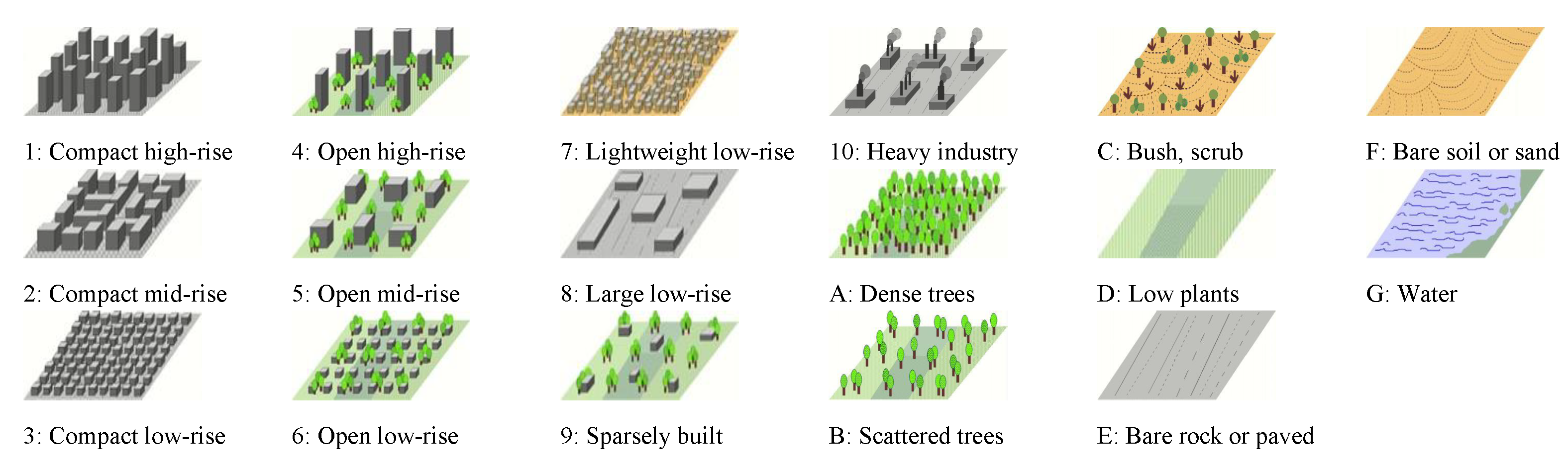
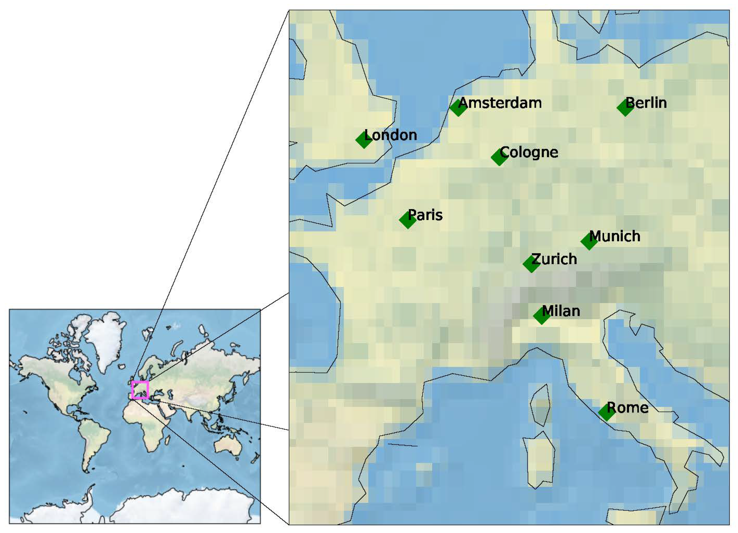
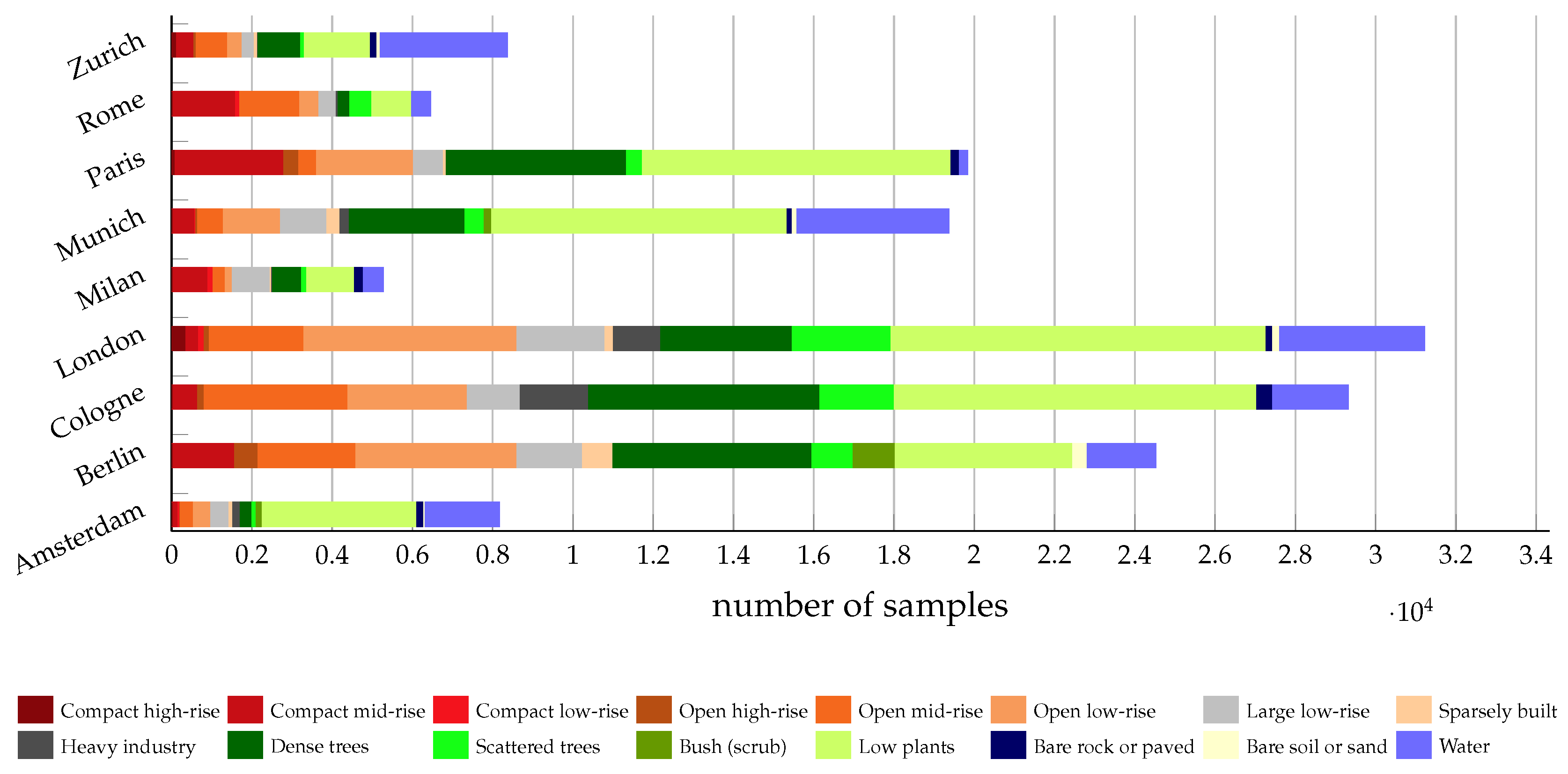
2.1. Study Areas and LCZ Dataset
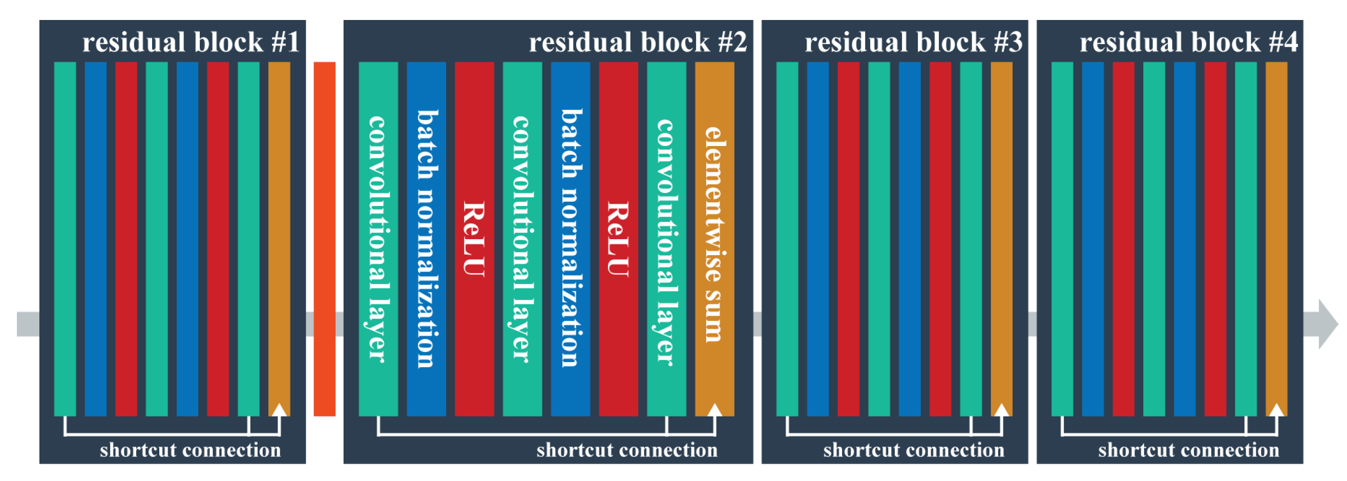
2.2. ResNet for LCZ Classification
2.3. Input Datasets and Features
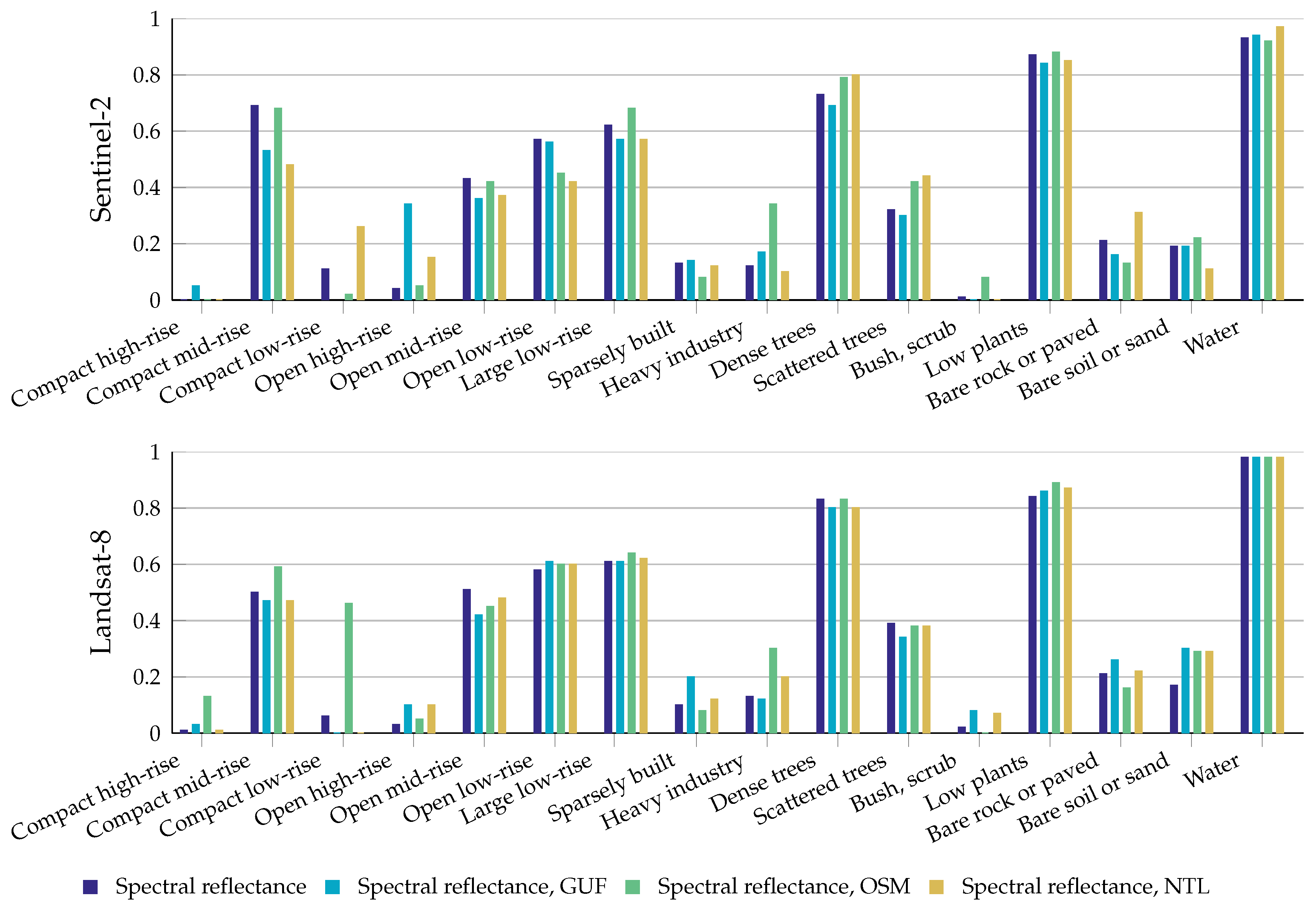
- Spectral reflectance:For each city, we have downloaded one cloud-free Sentinel-2 image and one Landsat-8 image from Google Earth Engine (GEE) [31]: Landsat-8 surface reflectance and Sentinel-2 MSI (TOA reflectance). Ten multispectral bands of Sentinel-2 imagery are used in this study: B2, B3, B4 and B8 with 10-m Ground Sampling Distance (GSD) and B5, B6, B7, B8a, B11 and B12 with 20-m GSD. The 20-m bands are up-sampled to 10-m GSD. The bands B1, B9 and B10 are not considered in this study because they contain mostly information about the atmosphere and thus bear little relevance to LCZ classification. Besides, nine multispectral bands of Landsat-8 imagery are also used: five Visible and Near-Infrared (VNIR) bands and two Short-Wave Infrared (SWIR) bands processed to orthorectified surface reflectance and two Thermal Infrared (TIR) bands processed to orthorectified brightness temperature. All Landsat-8 bands are up-sampled to 10-m GSD, in order to be aligned with Sentinel-2 images.
- Spectral indices:Spectral indices are extracted from both Sentinel-2 and Landsat-8 images. The well-established indices Normalized Difference Vegetation Index (NDVI), Enhanced Vegetation Index (EVI), Modified Normalized Difference Water Index (MNDWI) [32], Normalized Difference Built Index (NDBI) [33], Normalized Built-up Area Index (NBAI), Band Ratio for Built-up Area (BRBA) and Bare-Soil Index (BSI) are also considered [34], since they can provide indications about vegetation, water, buildings, soil, etc. [2].
- Other auxiliary data:In addition, we were allowed to access DLR’s Global Urban Footprint (GUF), a binary layer derived from TanDEM-X data, which indicates urban areas [19] globally. Besides, the Visible Infrared Imager Radiometer Suite (VIIRS)-based Nighttime Light (NTL) data are downloaded from GEE. Finally, we have downloaded the OpenStreetMap layers buildings and land use from OpenStreetMap Data Extracts (https://www.openstreetmap.org) for each city [35]. As auxiliary data, GUF, NTL and OSM are re-sampled to 10-m GSD.
2.4. Setup of Feature Importance Analysis for LCZ Classification
3. Results of Feature Importance Analysis
4. Improving LCZ Classification Accuracy with Proper Input Configurations
5. Discussion
5.1. Datasets and Feature Choice for LCZ Classification
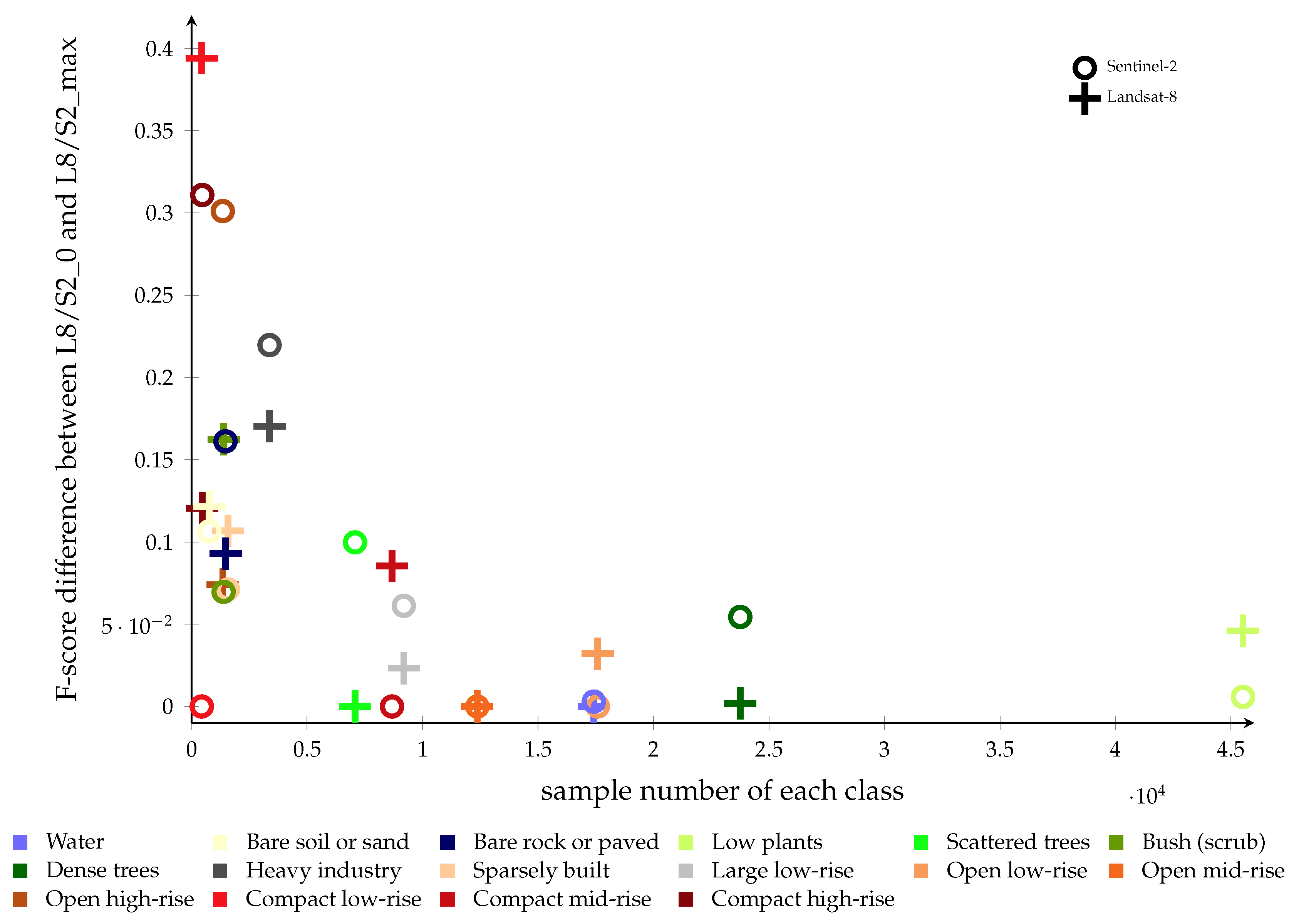
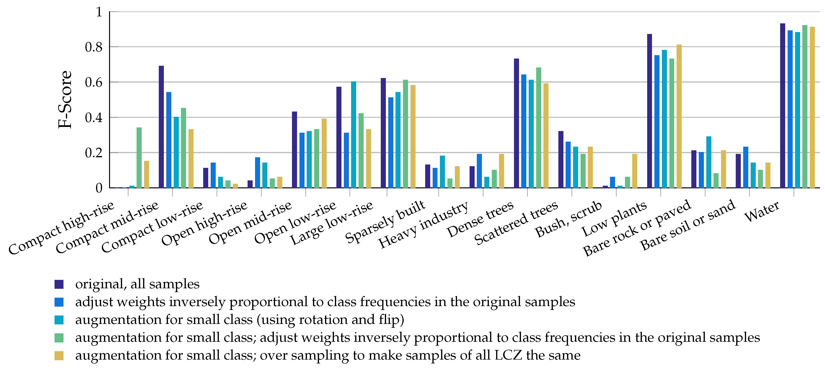
5.2. Class Imbalance Effect
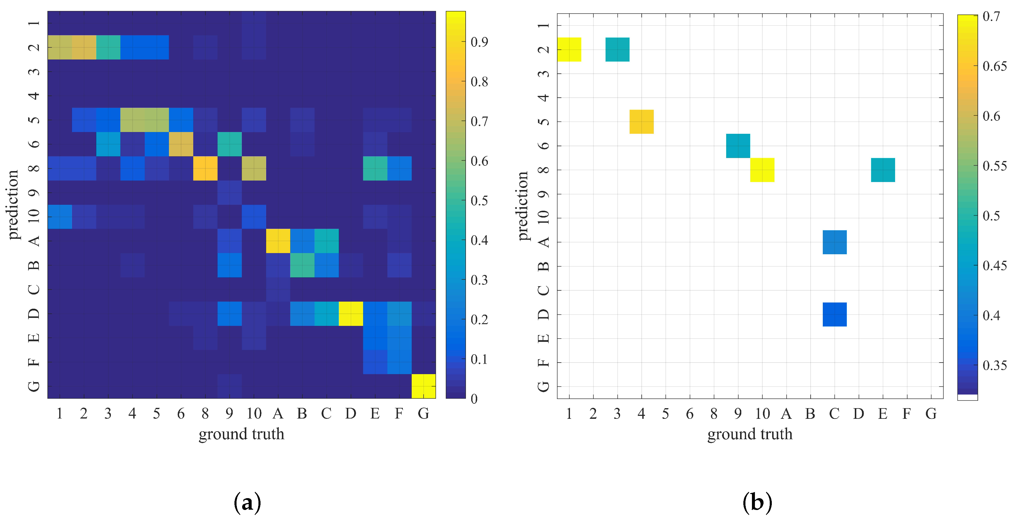
5.3. Confusion among LCZs
6. Summary and Conclusions
Author Contributions
Funding
Acknowledgments
Conflicts of Interest
References
- Stewart, I.D. Local climate zones: Origins, development, and application to urban heat island studies. In Proceedings of the Annual Meeting of the American Association of Geographers, Seattle, WA, USA, 12–16 April 2011. [Google Scholar]
- Bechtel, B.; Alexander, P.J.; Böhner, J.; Ching, J.; Conrad, O.; Feddema, J.; Mills, G.; See, L.; Stewart, I. Mapping local climate zones for a worldwide database of the form and function of cities. ISPRS Int. J. Geo-Inf. 2015, 4, 199–219. [Google Scholar] [CrossRef] [Green Version]
- Stewart, I.D.; Oke, T.R. Local climate zones for urban temperature studies. Bull. Am. Meteorol. Soc. 2012, 93, 1879–1900. [Google Scholar] [CrossRef]
- Stewart, I.D.; Oke, T.R.; Krayenhoff, E.S. Evaluation of the ‘local climate zone’scheme using temperature observations and model simulations. Int. J. Climatol. 2014, 34, 1062–1080. [Google Scholar] [CrossRef]
- Fenner, D.; Meier, F.; Bechtel, B.; Otto, M.; Scherer, D. Intra and inter local climate zone variability of air temperature as observed by crowdsourced citizen weather stations in Berlin, Germany. Meteorol. Z. 2017, 26, 525–547. [Google Scholar] [CrossRef]
- Quan, S.J.; Dutt, F.; Woodworth, E.; Yamagata, Y.; Yang, P.P.J. Local Climate Zone Mapping for Energy Resilience: A Fine-grained and 3D Approach. Energy Procedia 2017, 105, 3777–3783. [Google Scholar] [CrossRef]
- Quanz, J.A.; Ulrich, S.; Fenner, D.; Holtmann, A.; Eimermacher, J. Micro-scale variability of air temperature within a local climate zone in Berlin, Germany, during summer. Climate 2018, 6, 5. [Google Scholar] [CrossRef]
- Kotharkar, R.; Bagade, A. Evaluating urban heat island in the critical local climate zones of an Indian city. Landsc. Urban Plan. 2018, 169, 92–104. [Google Scholar] [CrossRef]
- Wicki, A.; Parlow, E. Attribution of local climate zones using a multitemporal land use/land cover classification scheme. J. Appl. Remote Sens. 2017, 11, 026001. [Google Scholar] [CrossRef] [Green Version]
- Taubenböck, H.; Esch, T.; Felbier, A.; Wiesner, M.; Roth, A.; Dech, S. Monitoring urbanization in mega cities from space. Remote Sens. Environ. 2012, 117, 162–176. [Google Scholar] [CrossRef]
- Wang, C.; Middel, A.; Myint, S.W.; Kaplan, S.; Brazel, A.J.; Lukasczyk, J. Assessing local climate zones in arid cities: The case of Phoenix, Arizona and Las Vegas, Nevada. ISPRS J. Photogramm. Remote Sens. 2018, 141, 59–71. [Google Scholar] [CrossRef]
- United Nations General Assembly. Transforming Our World: The 2030 Agenda for Sustainable Development; United Nations: New York, NY, USA, 2015. [Google Scholar]
- Danylo, O.; See, L.; Gomez, A.; Schnabel, G.; Fritz, S. Using the LCZ framework for change detection and urban growth monitoring. In Proceedings of the 19th EGU General Assembly, EGU2017, Vienna, Austria, 23–28 April 2017; Volume 19, p. 18043. [Google Scholar]
- Ho, H.C.; Lau, K.K.L.; Yu, R.; Wang, D.; Woo, J.; Kwok, T.C.Y.; Ng, E. Spatial variability of geriatric depression risk in a high-density city: A data-driven socio-environmental vulnerability mapping approach. Int. J. Environ. Res. Public Health 2017, 14, 994. [Google Scholar] [CrossRef] [PubMed]
- Yokoya, N.; Ghamisi, P.; Xia, J. Multimodal, multitemporal, and multisource global data fusion for local climate zones classification based on ensemble learning. In Proceedings of the 2017 IEEE International Geoscience and Remote Sensing Symposium (IGARSS), Fort Worth, TX, USA, 23–28 July 2017; pp. 1197–1200. [Google Scholar]
- Xu, Y.; Ma, F.; Meng, D.; Ren, C.; Leung, Y. A co-training approach to the classification of local climate zones with multi-source data. In Proceedings of the 2017 IEEE International Geoscience and Remote Sensing Symposium (IGARSS), Fort Worth, TX, USA, 23–28 July 2017; pp. 1209–1212. [Google Scholar]
- Esch, T.; Marconcini, M.; Felbier, A.; Roth, A.; Heldens, W.; Huber, M.; Schwinger, M.; Taubenböck, H.; Müller, A.; Dech, S. Urban footprint processor—Fully automated processing chain generating settlement masks from global data of the TanDEM-X mission. IEEE Geosci. Remote Sens. Lett. 2013, 10, 1617–1621. [Google Scholar] [CrossRef] [Green Version]
- Esch, T.; Taubenböck, H.; Roth, A.; Heldens, W.; Felbier, A.; Schmidt, M.; Mueller, A.A.; Thiel, M.; Dech, S.W. TanDEM-X mission-new perspectives for the inventory and monitoring of global settlement patterns. J. Appl. Remote Sens. 2012, 6, 061702. [Google Scholar] [CrossRef]
- Klotz, M.; Kemper, T.; Geiß, C.; Esch, T.; Taubenböck, H. How good is the map? A multi-scale cross-comparison framework for global settlement layers: Evidence from Central Europe. Remote Sens. Environ. 2016, 178, 191–212. [Google Scholar] [CrossRef] [Green Version]
- Shi, K.; Yu, B.; Huang, Y.; Hu, Y.; Yin, B.; Chen, Z.; Chen, L.; Wu, J. Evaluating the ability of NPP-VIIRS nighttime light data to estimate the gross domestic product and the electric power consumption of China at multiple scales: A comparison with DMSP-OLS data. Remote Sens. 2014, 6, 1705–1724. [Google Scholar] [CrossRef]
- Chen, Z.; Yu, B.; Hu, Y.; Huang, C.; Shi, K.; Wu, J. Estimating house vacancy rate in metropolitan areas using NPP-VIIRS nighttime light composite data. IEEE J. Sel. Top. Appl. Earth Obs. Remote Sens. 2015, 8, 2188–2197. [Google Scholar] [CrossRef]
- Sharma, R.C.; Tateishi, R.; Hara, K.; Gharechelou, S.; Iizuka, K. Global mapping of urban built-up areas of year 2014 by combining MODIS multispectral data with VIIRS nighttime light data. Int. J. Digit. Earth 2016, 9, 1004–1020. [Google Scholar] [CrossRef]
- Elvidge, C.D.; Baugh, K.; Zhizhin, M.; Hsu, F.C.; Ghosh, T. VIIRS night-time lights. Int. J. Remote Sens. 2017, 38, 5860–5879. [Google Scholar] [CrossRef] [Green Version]
- Wang, Q.; Zhang, F.; Li, X. Optimal Clustering Framework for Hyperspectral Band Selection. IEEE Trans. Geosci. Remote Sens. 2018, 56, 5910–5922. [Google Scholar] [CrossRef]
- Wang, Q.; He, X.; Li, X. Locality and Structure Regularized Low Rank Representation for Hyperspectral Image Classification. IEEE Trans. Geosci. Remote Sens. 2018. [Google Scholar] [CrossRef]
- Yokoya, N.; Ghamisi, P.; Xia, J.; Sukhanov, S.; Heremans, R.; Tankoyeu, I.; Bechtel, B.; Saux, B.L.; Moser, G.; Tuia, D. Open Data for Global Multimodal Land Use Classification: Outcome of the 2017 IEEE GRSS Data Fusion Contest. IEEE J. Sel. Top. Appl. Earth Obs. Remote Sens. 2018, 11, 1363–1377. [Google Scholar] [CrossRef]
- Radoux, J.; Chomé, G.; Jacques, D.C.; Waldner, F.; Bellemans, N.; Matton, N.; Lamarche, C.; D’Andrimont, R.; Defourny, P. Sentinel-2’s potential for sub-pixel landscape feature detection. Remote Sens. 2016, 8, 488. [Google Scholar] [CrossRef]
- He, K.; Zhang, X.; Ren, S.; Sun, J. Deep residual learning for image recognition. In Proceedings of the 2016 IEEE Conference on Computer Vision and Pattern Recognition Workshops (CVPRW), Las Vegas, NV, USA, 26 June–1 July 2016; pp. 770–778. [Google Scholar]
- Zhu, X.X.; Tuia, D.; Mou, L.; Xia, G.S.; Zhang, L.; Xu, F.; Fraundorfer, F. Deep learning in remote sensing: A comprehensive review and list of resources. IEEE Geosci. Remote Sens. Mag. 2017, 5, 8–36. [Google Scholar] [CrossRef]
- Zhu, X.X. So2Sat LCZ42: A Benchmark Dataset for Local Climate Zones Classification. 2018. to appear. [Google Scholar]
- Gorelick, N.; Hancher, M.; Dixon, M.; Ilyushchenko, S.; Thau, D.; Moore, R. Google Earth Engine: Planetary-scale geospatial analysis for everyone. Remote Sens. Environ. 2017, 202, 18–27. [Google Scholar] [CrossRef]
- Ji, L.; Geng, X.; Sun, K.; Zhao, Y.; Gong, P. Target detection method for water mapping using Landsat-8 OLI/TIRS imagery. Water 2015, 7, 794–817. [Google Scholar] [CrossRef]
- Zha, Y.; Gao, J.; Ni, S. Use of normalized difference built-up index in automatically mapping urban areas from TM imagery. Int. J. Remote Sens. 2003, 24, 583–594. [Google Scholar] [CrossRef]
- Tucker, C.J. Red and photographic infrared linear combinations for monitoring vegetation. Remote Sens. Environ. 1979, 8, 127–150. [Google Scholar] [CrossRef] [Green Version]
- OpenStreetMap Contributors. 2017. Available online: https://www.openstreetmap.org (accessed on 30 September 2018).
- Bechtel, B.; Demuzere, M.; Sismanidis, P.; Fenner, D.; Brousse, O.; Beck, C.; Van Coillie, F.; Conrad, O.; Keramitsoglou, I.; Middel, A.; et al. Quality of Crowdsourced Data on Urban Morphology—The Human Influence Experiment (HUMINEX). Urban Sci. 2017, 1, 15. [Google Scholar] [CrossRef]
- Qiu, C.; Schmitt, M.; Ghamisi, P.; Zhu, X. Effect of the training set configuration on sentinel-2-based urban local climate zone classification. In Proceedings of the International Archives of the Photogrammetry, Remote Sensing & Spatial Information Sciences, Riva del Garda, Italy, 4–7 June 2018; Volume 42. [Google Scholar]
- Mou, L.; Bruzzone, L.; Zhu, X.X. Learning spectral-spatial-temporal features via a recurrent convolutional neural network for change detection in multispectral imagery. arXiv, 2018; arXiv:1803.02642. [Google Scholar]
- Wang, Q.; Liu, S.; Chanussot, J.; Li, X. Scene Classification with Recurrent Attention of VHR Remote Sensing Images. IEEE Trans. Geosci. Remote Sens. 2018, 99, 1–13. [Google Scholar] [CrossRef]


| Data and Feature | Dataset | |
|---|---|---|
| Sentinel-2 | Landsat-8 | |
| Spectral reflectance | S_0 | L_0 |
| Spectral reflectance, Indices | S_1 | L_1 |
| Spectral reflectance, GUF | S_2 | L_2 |
| Spectral reflectance, OSM | S_3 | L_3 |
| Spectral reflectance, NTL | S_4 | L_4 |
| Spectral reflectance, GUF, OSM | S_5 | L_5 |
| Input | Sentinel-2 | Landsat-8 | Stacking | ||||||||||
|---|---|---|---|---|---|---|---|---|---|---|---|---|---|
| S_0 | S_1 | S_2 | S_3 | S_4 | S_5 | L_0 | L_1 | L_2 | L_3 | L_4 | L_5 | S_0 + L_0 | |
| OA | 0.71 | 0.63 | 0.67 | 0.71 | 0.68 | 0.71 | 0.72 | 0.58 | 0.70 | 0.73 | 0.71 | 0.73 | 0.72 |
| WA | 0.93 | 0.90 | 0.93 | 0.94 | 0.92 | 0.94 | 0.93 | 0.87 | 0.94 | 0.94 | 0.93 | 0.94 | 0.93 |
| AA | 0.46 | 0.41 | 0.45 | 0.49 | 0.46 | 0.50 | 0.48 | 0.37 | 0.47 | 0.50 | 0.48 | 0.50 | 0.48 |
| Kappa | 0.65 | 0.56 | 0.59 | 0.64 | 0.61 | 0.65 | 0.67 | 0.50 | 0.64 | 0.68 | 0.65 | 0.67 | 0.65 |
| Data, Method | OA | WA | AA | Kappa | |
|---|---|---|---|---|---|
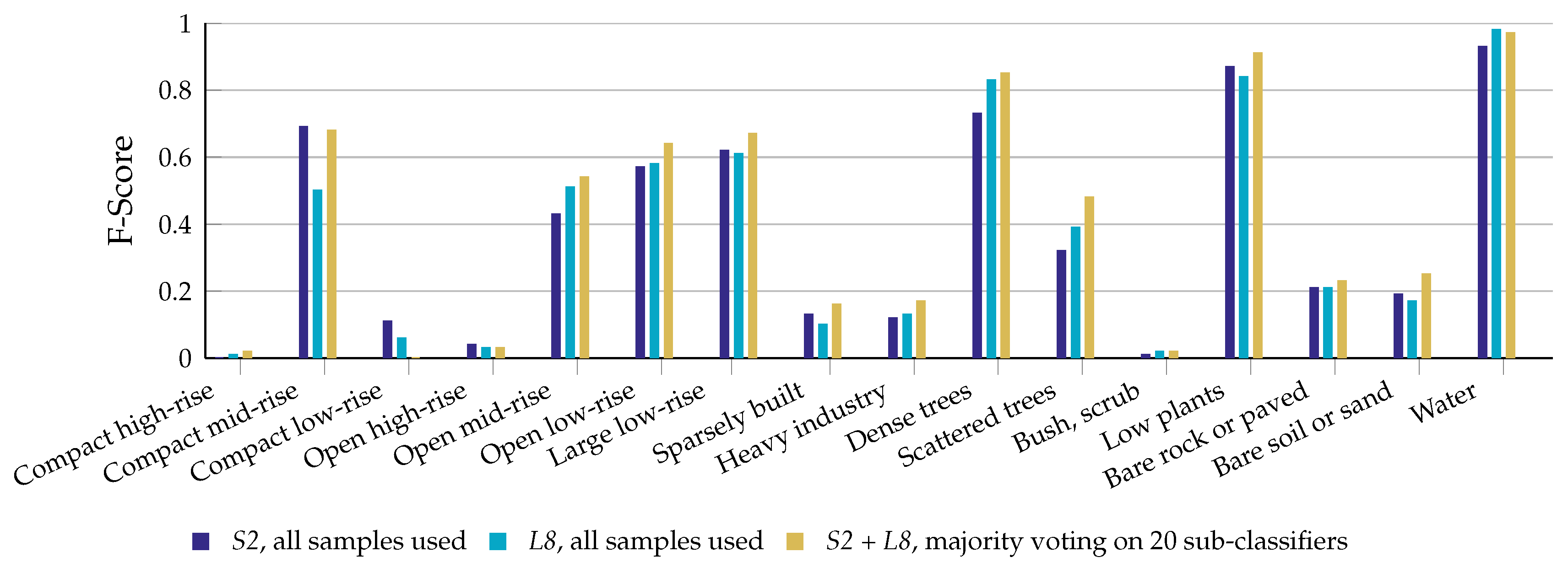
| S2 | all samples used (S2_0) | 0.71 | 0.93 | 0.46 | 0.65 |
| majority voting on 10 sub-classifiers | 0.72 | 0.94 | 0.51 | 0.65 | |
| L8 | all samples used (L8_0) | 0.72 | 0.93 | 0.48 | 0.67 |
| majority voting on 10 sub-classifiers | 0.75 | 0.94 | 0.45 | 0.70 | |
| S2 + L8 | majority voting on 20 sub-classifiers | 0.78 | 0.95 | 0.51 | 0.73 |
| City | OA | WA | AA | Kappa |
|---|---|---|---|---|
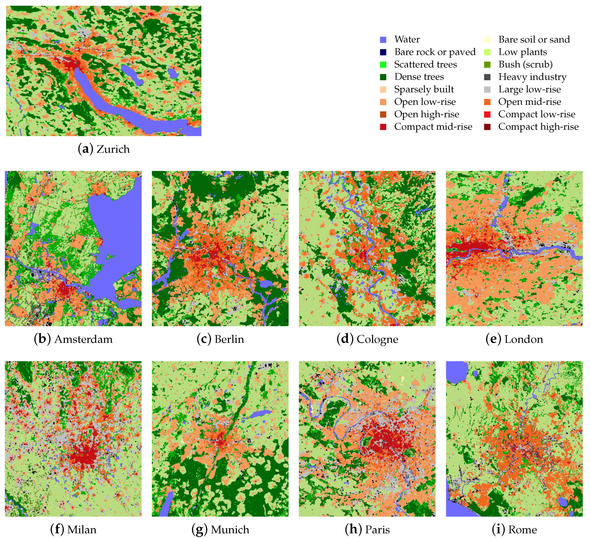
| Amsterdam | 0.65 | 0.92 | 0.47 | 0.55 |
| Berlin | 0.76 | 0.96 | 0.54 | 0.72 |
| Cologne | 0.78 | 0.96 | 0.49 | 0.73 |
| London | 0.80 | 0.95 | 0.53 | 0.76 |
| Milan | 0.83 | 0.96 | 0.50 | 0.80 |
| Munich | 0.88 | 0.97 | 0.57 | 0.85 |
| Paris | 0.82 | 0.96 | 0.38 | 0.76 |
| Rome | 0.62 | 0.92 | 0.45 | 0.56 |
| Zurich | 0.85 | 0.96 | 0.64 | 0.80 |
| MEAN | 0.78 | 0.95 | 0.51 | 0.73 |
© 2018 by the authors. Licensee MDPI, Basel, Switzerland. This article is an open access article distributed under the terms and conditions of the Creative Commons Attribution (CC BY) license (http://creativecommons.org/licenses/by/4.0/).
Share and Cite
Qiu, C.; Schmitt, M.; Mou, L.; Ghamisi, P.; Zhu, X.X. Feature Importance Analysis for Local Climate Zone Classification Using a Residual Convolutional Neural Network with Multi-Source Datasets. Remote Sens. 2018, 10, 1572. https://doi.org/10.3390/rs10101572
Qiu C, Schmitt M, Mou L, Ghamisi P, Zhu XX. Feature Importance Analysis for Local Climate Zone Classification Using a Residual Convolutional Neural Network with Multi-Source Datasets. Remote Sensing. 2018; 10(10):1572. https://doi.org/10.3390/rs10101572
Chicago/Turabian StyleQiu, Chunping, Michael Schmitt, Lichao Mou, Pedram Ghamisi, and Xiao Xiang Zhu. 2018. "Feature Importance Analysis for Local Climate Zone Classification Using a Residual Convolutional Neural Network with Multi-Source Datasets" Remote Sensing 10, no. 10: 1572. https://doi.org/10.3390/rs10101572