Improving the Reliability of Mixture Tuned Matched Filtering Remote Sensing Classification Results Using Supervised Learning Algorithms and Cross-Validation


Abstract
:
1. Introduction
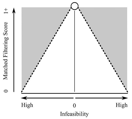
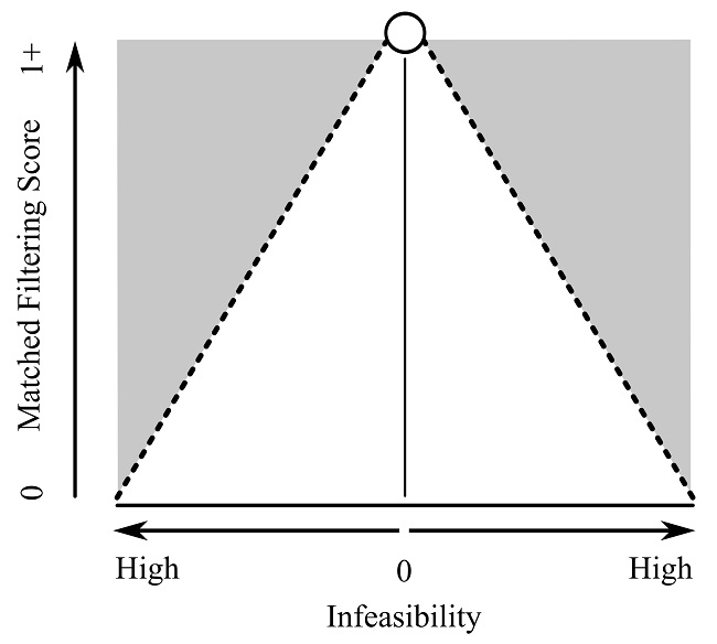
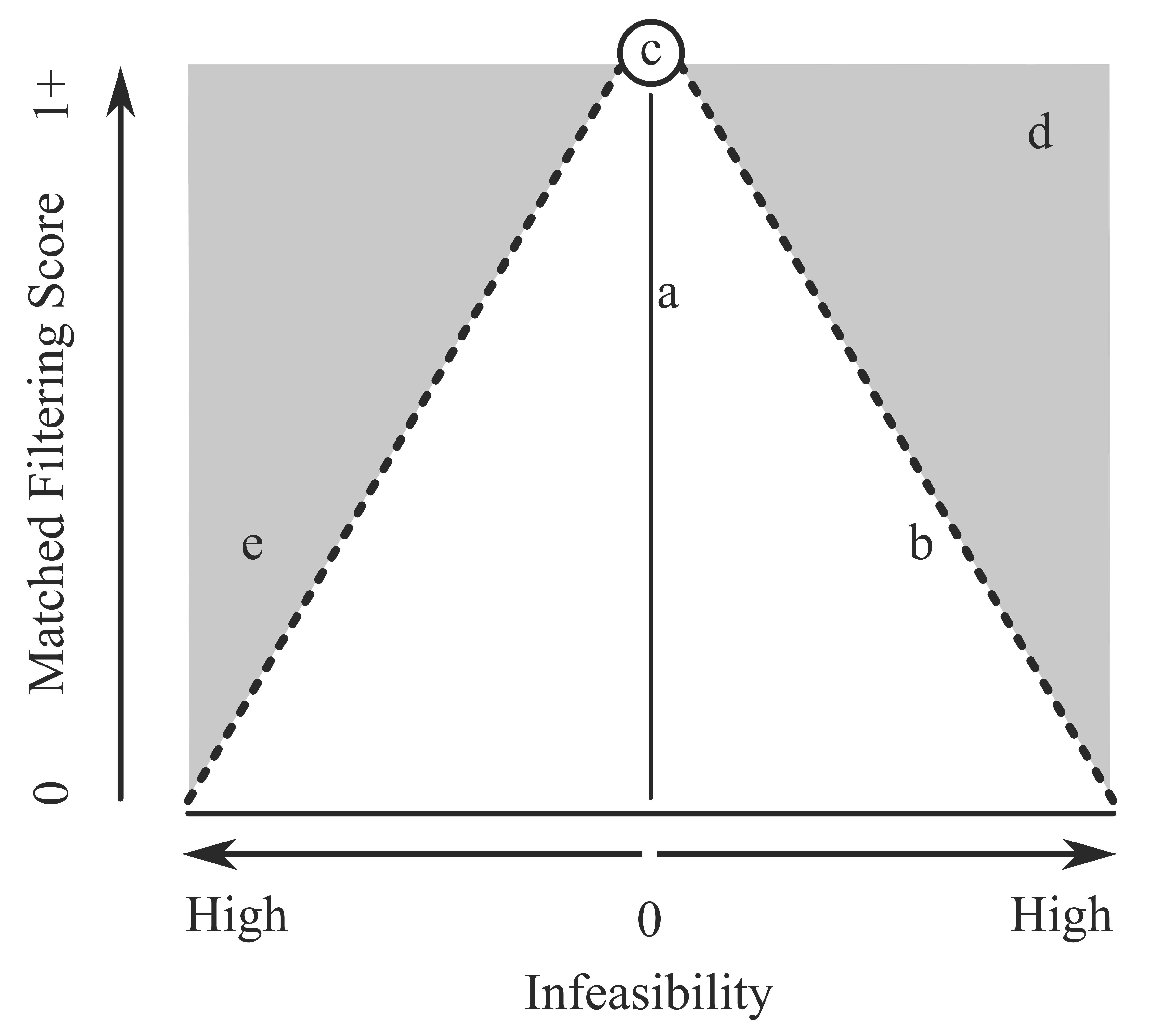
Background: MTMF
2. Materials and Methods
2.1. Accuracy Assessment via Supervised Learning Algorithms
2.1.1. Overview
2.1.2. Supervised Learning Algorithms and Cross-validation
2.2. Study Site, Image Acquisition and Processing, Field Sampling, and Classification Overview
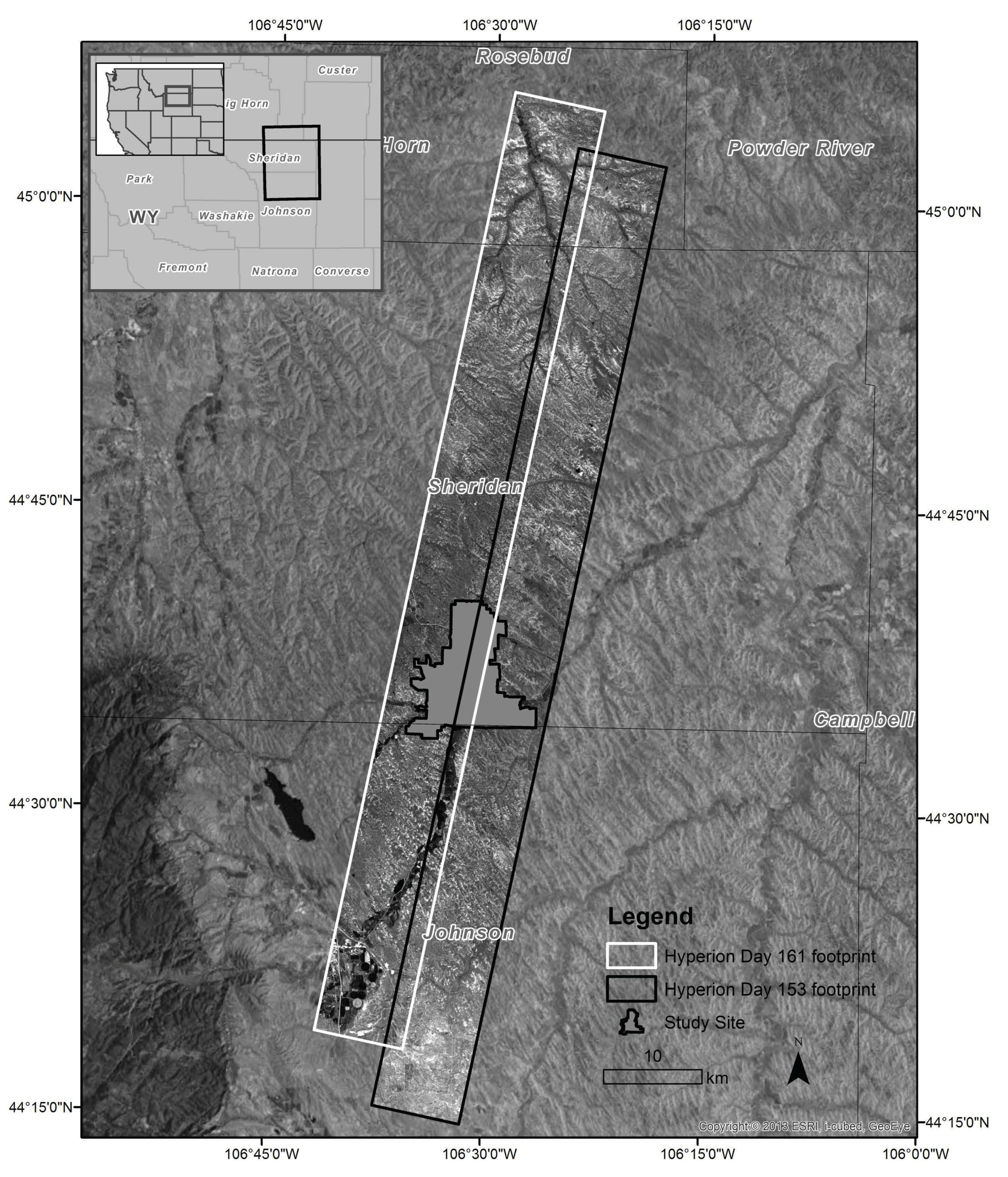
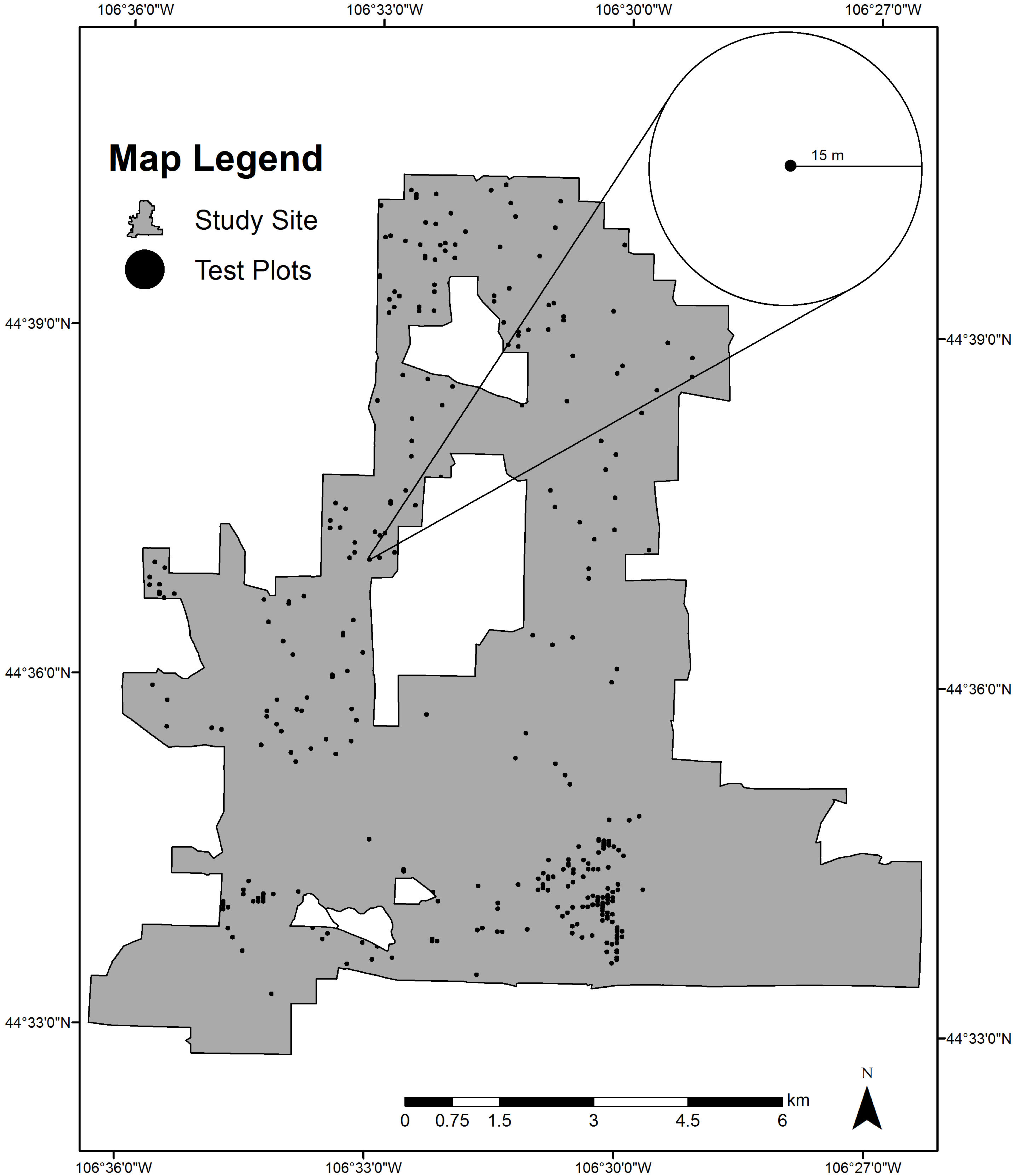
2.2.1. Study Site
2.2.2. Hyperion Data and Tasking
2.2.3. Data Pre-Processing
2.2.4. Target Spectra and Reference Plot Collection
2.2.5. MTMF Classification
2.2.6. Georeferencing and Post-Processing
3. Results
Overall Accuracy and Kappa Accuracy Results
4. Discussion
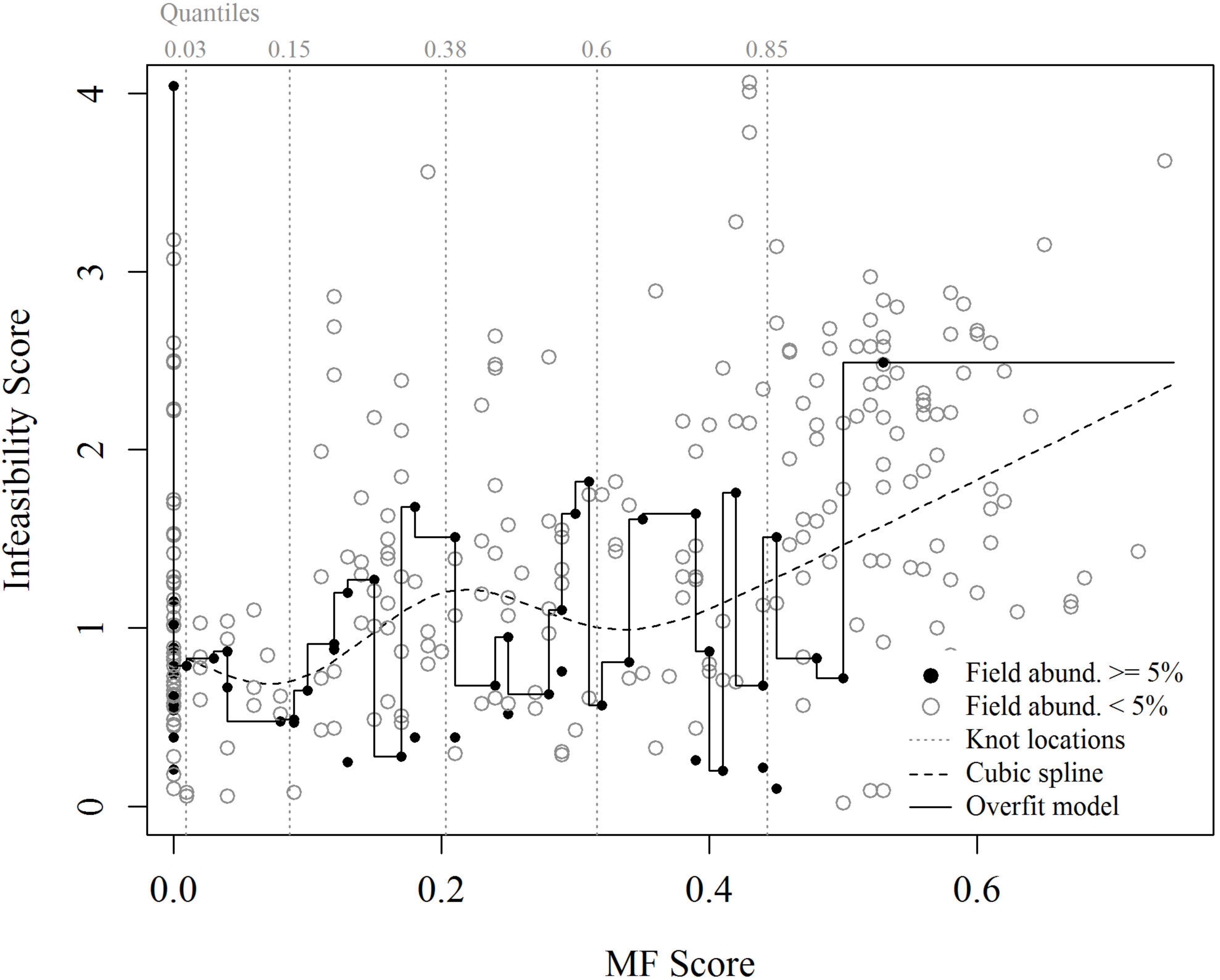
4.1. Inflation of Map Accuracy
4.2. Hyperion, Automation
5. Conclusions
Author Contributions
Funding
Acknowledgments
Conflicts of Interest
References
- Boardman, J.W.; Kruse, F.A. Analysis of imaging spectrometer data using N-dimensional geometry and a mixture-tuned matched filtering approach. IEEE Trans. Geosci. Remote Sens. 2011, 49, 4138–4152. [Google Scholar] [CrossRef]
- Boardman, J.W. Leveraging the high dimensionality of AVIRIS data for improved sub-pixel target unmixing and rejection of false positives: Mixture tuned matched filtering. In Proceedings of the Summaries of the Seventh JPL Airborne Geoscience Workshop; JPL: Pasadena, CA, USA, 1998; pp. 55–56. [Google Scholar]
- Parker Williams, A.E.; Hunt, E.R., Jr. Estimation of leafy spurge cover from hyperspectral imagery using mixture tuned matched filtering. Remote Sens. Environ. 2002, 82, 446–456. [Google Scholar] [CrossRef]
- Glenn, N.F.; Mundt, J.T.; Weber, K.T.; Prather, T.S.; Lass, L.W.; Pettingill, J. Hyperspectral data processing for repeat detection of small infestations of leafy spurge. Remote Sens. Environ. 2005, 95, 399–412. [Google Scholar] [CrossRef]
- Wang, J.-J.; Zhou, G.; Zhang, Y.; Bussink, C.; Zhang, J.; Ge, H. An unsupervised mixture-tuned matched filtering-based method for the remote sensing of opium poppy fields using EO-1 Hyperion data: An example from Helmand, Afghanistan. Remote Sens. Lett. 2016, 7, 945–954. [Google Scholar] [CrossRef]
- Boardman, J.W. Automating spectral unmixing of AVIRIS data using convex geometry concepts. In Proceedings of the 4th JPL Airborne Geoscience Workshop, Pasadena, CA, USA, 25–29 October 1993; pp. 11–14. [Google Scholar]
- Green, A.A.; Berman, M.; Switzer, P.; Craig, M.D. A transformation for ordering multispectral data in terms of image quality with implications for noise removal. IEEE Trans. Geosci. Remote Sens. 1988, 26, 65–74. [Google Scholar] [CrossRef] [Green Version]
- Mundt, J.T.; Streutker, D.R.; Glenn, N.F. Partial unmixing of hyperspectral imagery: Theory and methods. In Proceedings of the American Society of Photogrammetry and Remote Sensing, Tampa, FL, USA, 7–11 May 2007. [Google Scholar]
- Chang, C.-I. Hyperspectral Imaging: Techniques for Spectral Detection and Classification; Springer Science & Business Media: New York, NY, USA, 2003; Volume 1. [Google Scholar]
- Heinz, D.C. Fully constrained least squares linear spectral mixture analysis method for material quantification in hyperspectral imagery. IEEE Trans. Geosci. Remote Sens. 2001, 39, 529–545. [Google Scholar] [CrossRef]
- Okin, G.S.; Roberts, D.A.; Murray, B.; Okin, W.J. Practical limits on hyperspectral vegetation discrimination in arid and semiarid environments. Remote Sens. Environ. 2001, 77, 212–225. [Google Scholar] [CrossRef]
- Settle, J.J.; Drake, N.A. Linear mixing and the estimation of ground cover proportions. Int. J. Remote Sens. 1993, 14, 1159–1177. [Google Scholar] [CrossRef] [Green Version]
- Mitchell, J.J.; Glenn, N.F. Subpixel abundance estimates in mixture-tuned matched filtering classifications of leafy spurge (Euphorbia esula L.). Int. J. Remote Sens. 2009, 30, 6099–6119. [Google Scholar] [CrossRef]
- Carrino, T.A.; Crósta, A.P.; Toledo, C.L.B.; Silva, A.M. Hyperspectral remote sensing applied to mineral exploration in Southern Peru: A multiple data integration approach in the chapi chiara gold prospect. Int. J. Appl. Earth Observ. Geoinf. 2018, 64, 287–300. [Google Scholar] [CrossRef]
- Dos Reis Salles, R.; De Souza Filho, C.R.; Cudahy, T.; Vicente, L.E.; Monteiro, L.V.S. Hyperspectral remote sensing applied to uranium exploration: A case study at the Mary Kathleen metamorphic-hydrothermal U-REE deposit, NW, Queensland, Australia. J. Geochem. Explor. 2017, 179, 36–50. [Google Scholar] [CrossRef]
- Calin, M.-A.; Coman, T.; Parasca, S.V.; Bercaru, N.; Savastru, R.S.; Manea, D. Hyperspectral imaging-based wound analysis using mixture-tuned matched filtering classification method. J. Biomed. Opt. 2015, 20, 046004. [Google Scholar] [CrossRef] [PubMed]
- Anderson, G.L.; Everitt, J.H.; Escobar, D.E.; Spencer, N.R.; Andrascik, R.J. Mapping leafy spurge (Euphorbia esula) infestations using aerial photography and geographic information systems. Geocarto Int. 1996, 11, 81–89. [Google Scholar] [CrossRef]
- Casady, G.M.; Hanley, R.S.; Seelan, S.K. Detection of leafy spurge (Euphorbia esula) using multidate high-resolution satellite imagery. Weed Technol. 2005, 19, 462–467. [Google Scholar] [CrossRef]
- Dudek, K.B.; Root, R.R.; Kokaly, R.F.; Anderson, G.L. Increased spatial and temporal consistency of leafy spurge maps from multidate AVIRIS imagery: A modified, hybrid linear spectral mixture analysis/mixture-tuned matched filtering approach. In Proceedings of the 13th JPL Airborne Earth Sciences Workshop, Tampa, FL, USA, 7–11 May 2007. [Google Scholar]
- Everitt, J.H.; Anderson, G.L.; Escobar, D.E.; Davis, M.R.; Spencer, N.R.; Andrascik, R.J. Use of remote sensing for detecting and mapping leafy spurge (Euphorbia esula). Weed Technol. 1995, 9, 599–609. [Google Scholar] [CrossRef]
- Hunt, E.R., Jr.; Parker Williams, A.E. Comparison of AVIRIS and multispectral remote sensing for detection of leafy spurge. In Proceedings of the 13th JPL Airborne Earth Sciences Workshop, Tampa, FL, USA, 7–11 May 2007. [Google Scholar]
- Hunt, E.R., Jr.; Parker Williams, A.E. Detection of flowering leafy spurge with satellite multispectral imagery. Rangel. Ecol. Manag. 2006, 59, 494–499. [Google Scholar] [CrossRef]
- Hunt, E.R., Jr.; Everitt, J.H.; Ritchie, J.C.; Moran, M.S.; Booth, D.T.; Anderson, G.L.; Clark, P.E.; Seyfried, M.S. Applications and research using remote sensing for rangeland management. Photogramm. Eng. Remote Sens. 2003, 69, 675–693. [Google Scholar] [CrossRef]
- Kokaly, R.F.; Root, R.R.; Brown, K.; Anderson, G.L.; Hager, S. Mapping the invasive species leafy spurge (Euphorbia esula) in Theodore Roosevelt National Park using field measurements of vegetation spectra and imaging spectroscopy data. In Proceedings of the 2002 Denver Annual Meeting, Denver, CO, USA, 18–20 February 2002. [Google Scholar]
- Kokaly, R.F.; Anderson, G.L.; Root, R.R.; Brown, K.E.; Mladinich, C.S.; Hager, S.; Dudek, K.B. Mapping leafy spurge by identifying signatures of vegetation field spectra in compact airborne spectrographic imager (CASI) data. In Proceedings of the Society for Range Management 57th Annual Meeting, Salt Lake City, UT, USA, 10–14 February 2004; pp. 249–260. [Google Scholar]
- Lawrence, R.L.; Wood, S.D.; Sheley, R.L. Mapping invasive plants using hyperspectral imagery and Breiman Cutler classifications (RandomForest). Remote Sens. Environ. 2006, 100, 356–362. [Google Scholar] [CrossRef]
- Parker Williams, A.E.; Hunt, E.R., Jr. Accuracy assessment for detection of leafy spurge with hyperspectral imagery. J. Range Manag. 2004, 57, 106–112. [Google Scholar] [CrossRef]
- Parker Williams, A.E. Biological Control and Hyperspectral Remote Sensing of Leafy Spurge (Euphorbia esula L.) an Exotic Plant Species in North America. Ph.D. Thesis, University of Wyoming, Laramie, WY, USA, 2001. [Google Scholar]
- Root, R.R.; Anderson, G.L.; Hager, S.N.; Brown, K.E.; Dudek, K.B.; Kokaly, R.F. Application of advanced remote sensing and modeling techniques for the detection and management of leafy spurge: Challenges and opportunities. In Proceedings of the Society for Range Management 57th Annual Meeting, Salt Lake City, UT, USA, 10–14 February 2004; pp. 24–30. [Google Scholar]
- Babu, M.J.R.; Rao, E.N.D.; Kallempudi, L.; Chandra, D.I. Mapping of Aluminous Rich Laterite Depositions through Hyper Spectral Remote Sensing. Int. J. Geosci. 2018, 9, 93–105. [Google Scholar] [CrossRef]
- Gregoire, T.G.; Valentine, H.T. Sampling Strategies for Natural Resources and the Environment; Chapman and Hall/CRC: Boca Raton, FL, USA, 2004. [Google Scholar]
- Mannel, S.; Price, M.; Hua, D. Impact of reference datasets and autocorrelation on classification accuracy. Int. J. Remote Sens. 2011, 32, 5321–5330. [Google Scholar] [CrossRef]
- Duro, D.C.; Franklin, S.E.; Dubé, M.G. A comparison of pixel-based and object-based image analysis with selected machine learning algorithms for the classification of agricultural landscapes using SPOT-5 HRG imagery. Remote Sens. Environ. 2012, 118, 259–272. [Google Scholar] [CrossRef]
- Huang, C.; Davis, L.S.; Townshend, J.R.G. An assessment of support vector machines for land cover classification. Int. J. Remote Sens. 2002, 23, 725–749. [Google Scholar] [CrossRef]
- Jenks, G.F. The data model concept in statistical mapping. Int. Yearbook Cartogr. 1967, 7, 186–190. [Google Scholar]
- Routh, D.; Seegmiller, L. Mixture Tuned Match Filtering (MTMF) Classification (MTMF_V.1.0): Raw Google Earth Engine Algorithm Code. Ucross High Plains Stewardship Initiative. 2015. Available online: https://code.earthengine.google.com/c66847b2b0ed5c332a912c94bdb8f05c (accessed on 23 October 2018).
- Aspinall, R.J. Use of logistic regression for validation of maps of the spatial distribution of vegetation species derived from high spatial resolution hyperspectral remotely sensed data. Ecol. Model. 2002, 157, 301–312. [Google Scholar] [CrossRef]
- Caruana, R.; Niculescu-Mizil, A. An empirical comparison of supervised learning algorithms. In Proceedings of the 23rd International Conference on Machine Learning, Pittsburgh, PA, USA, 25–29 June 2006; pp. 161–168. [Google Scholar]
- Rogan, J.; Franklin, J.; Stow, D.; Miller, J.; Woodcock, C.; Roberts, D. Mapping land-cover modifications over large areas: A comparison of machine learning algorithms. Remote Sens. Environ. 2008, 112, 2272–2283. [Google Scholar] [CrossRef]
- Srivastava, P.K.; Han, D.; Rico-Ramirez, M.A.; Bray, M.; Islam, T. Selection of classification techniques for land use/land cover change investigation. Adv. Space Res. 2012, 50, 1250–1265. [Google Scholar] [CrossRef]
- Vink, J.P.; De Haan, G. Comparison of machine learning techniques for target detection. Artif. Intell. Rev. 2015, 43, 125–139. [Google Scholar] [CrossRef]
- Bioucas-Dias, J.M.; Plaza, A.; Camps-Valls, G.; Scheunders, P.; Nasrabadi, N.; Chanussot, J. Hyperspectral remote sensing data analysis and future challenges. IEEE Geosci. Remote Sens. Mag. 2013, 1, 6–36. [Google Scholar] [CrossRef]
- Camps-Valls, G.; Gómez-Chova, L.; Calpe-Maravilla, J.; Martín-Guerrero, J.D.; Soria-Olivas, E.; Alonso-Chordá, L.; Moreno, J. Robust support vector method for hyperspectral data classification and knowledge discovery. IEEE Trans. Geosci. Remote Sens. 2004, 42, 1530–1542. [Google Scholar] [CrossRef] [Green Version]
- Melgani, F.; Bruzzone, L. Classification of hyperspectral remote sensing images with support vector machines. IEEE Trans. Geosci. Remote Sens. 2004, 42, 1778–1790. [Google Scholar] [CrossRef] [Green Version]
- Mountrakis, G.; Im, J.; Ogole, C. Support vector machines in remote sensing: A review. ISPRS J. Photogramm. Remote Sens. 2011, 66, 247–259. [Google Scholar] [CrossRef]
- Erol, H.; Tyoden, B.M.; Erol, R. Classification performances of data mining clustering algorithms for remotely sensed multispectral image data. In Proceedings of the 2018 Innovations in Intelligent Systems and Applications (INISTA), Thessaloniki, Greece, 3–5 July 2018; pp. 1–4. [Google Scholar]
- Siedliska, A.; Baranowski, P.; Zubik, M.; Mazurek, W.; Sosnowska, B. Detection of fungal infections in strawberry fruit by VNIR/SWIR hyperspectral imaging. Postharvest Biol. Technol. 2018, 139, 115–126. [Google Scholar] [CrossRef]
- Rodriguez-Galiano, V.F.; Chica-Olmo, M.; Abarca-Hernandez, F.; Atkinson, P.M.; Jeganathan, C. Random Forest classification of Mediterranean land cover using multi-seasonal imagery and multi-seasonal texture. Remote Sens. Environ. 2012, 121, 93–107. [Google Scholar] [CrossRef]
- Belgiu, M.; Drăguţ, L. Random forest in remote sensing: A review of applications and future directions. ISPRS J. Photogramm. Remote Sens. 2016, 114, 24–31. [Google Scholar] [CrossRef]
- Pullanagari, R.; Kereszturi, G.; Yule, I. Integrating airborne hyperspectral, topographic, and soil data for estimating pasture quality using recursive feature elimination with random forest regression. Remote Sens. 2018, 10, 1117. [Google Scholar] [CrossRef]
- Son, N.-T.; Chen, C.-F.; Chen, C.-R.; Minh, V.-Q. Assessment of Sentinel-1A data for rice crop classification using random forests and support vector machines. Geocarto Int. 2018, 33, 587–601. [Google Scholar] [CrossRef]
- Atkinson, P.M.; Tatnall, A.R.L. Introduction neural networks in remote sensing. Int. J. Remote Sens. 1997, 18, 699–709. [Google Scholar] [CrossRef]
- Paola, J.D.; Schowengerdt, R.A. A review and analysis of backpropagation neural networks for classification of remotely-sensed multi-spectral imagery. Int. J. Remote Sens. 1995, 16, 3033–3058. [Google Scholar] [CrossRef]
- Zhu, X.X.; Tuia, D.; Mou, L.; Xia, G.-S.; Zhang, L.; Xu, F.; Fraundorfer, F. Deep learning in remote sensing: A comprehensive review and list of resources. IEEE Geosci. Remote Sens. Mag. 2017, 5, 8–36. [Google Scholar] [CrossRef]
- Debella-Gilo, M.; Etzelmüller, B. Spatial prediction of soil classes using digital terrain analysis and multinomial logistic regression modeling integrated in GIS: Examples from Vestfold County, Norway. Catena 2009, 77, 8–18. [Google Scholar] [CrossRef]
- Afshar, F.A.; Ayoubi, S.; Jafari, A. The extrapolation of soil great groups using multinomial logistic regression at regional scale in arid regions of Iran. Geoderma 2018, 315, 36–48. [Google Scholar] [CrossRef]
- Bandos, T.V.; Bruzzone, L.; Camps-Valls, G. Classification of hyperspectral images with regularized linear discriminant analysis. IEEE Trans. Geosci. Remote Sens. 2009, 47, 862–873. [Google Scholar] [CrossRef]
- Eikvil, L.; Aurdal, L.; Koren, H. Classification-based vehicle detection in high-resolution satellite images. ISPRS J. Photogramm. Remote Sens. 2009, 64, 65–72. [Google Scholar] [CrossRef]
- Kohavi, R. A study of cross-validation and bootstrap for accuracy estimation and model selection. In Proceedings of the International Joint Conference on Artificial Intelligence, Montreal, CA, USA, 20–25 August 1995; pp. 1137–1145. [Google Scholar]
- R Development Core Team. R: A Language and Environment for Statistical Computing; R Foundation for Statistical Computing: Vienna, Austria, 2016. [Google Scholar]
- Kuhn, M. Package ‘Caret’, v6.0-80. The Comprehensive R Archive Network (CRAN). 2018, p. 213. Available online: https://cran.r-project.org/ (accessed on 23 October 2018).
- Kuhn, M. Building predictive models in R using the caret package. J. Stat. Softw. 2008, 28, 1–26. [Google Scholar] [CrossRef]
- Gudex-Cross, D.; Pontius, J.; Adams, A. Enhanced forest cover mapping using spectral unmixing and object-based classification of multi-temporal Landsat imagery. Remote Sens. Environ. 2017, 196, 193–204. [Google Scholar] [CrossRef]
- Mikheeva, A.I.; Tutubalina, O.V.; Zimin, M.V.; Golubeva, E.I. A Subpixel Classification of Multispectral Satellite Imagery for Interpetation of Tundra-Taiga Ecotone Vegetation (Case Study on Tuliok River Valley, Khibiny, Russia). Izvestiya Atmos. Ocean. Phys. 2017, 53, 1164–1173. [Google Scholar] [CrossRef]
- ENVI, v. 5.1; Exelis Visual Information Solutions: Boulder, CO, USA, 2015.
- Lym, R.G. The biology and integrated management of leafy spurge (Euphorbia esula) on North Dakota rangeland. Weed Technol. 1998, 12, 367–373. [Google Scholar] [CrossRef]
- Mooney, H.A.; Cleland, E.E. The evolutionary impact of invasive species. Proc. Natl. Acad. Sci. USA 2001, 98, 5446–5451. [Google Scholar] [CrossRef] [PubMed] [Green Version]
- Walker, J.W.; Kronberg, S.L.; Al-Rowaily, S.L.; West, N.E. Comparison of sheep and goat preferences for leafy spurge. J. Range Manag. 1994, 429–434. [Google Scholar] [CrossRef]
- Pearlman, J.S.; Barry, P.S.; Segal, C.C.; Shepanski, J.; Beiso, D.; Carman, S.L. Hyperion, a space-based imaging spectrometer. IEEE Trans. Geosci. Remote Sens. 2003, 41, 1160–1173. [Google Scholar] [CrossRef]
- Hunt, E.R.; McMurtrey, J.E.; Parker Williams, A.E. Spectral characteristics of leafy spurge (Euphorbia esula) leaves and flower bracts. Weed Sci. 2004, 52, 492–497. [Google Scholar] [CrossRef]
- Perkins, T.; Adler-Golden, S.; Cappelaere, P.; Mandl, D. High-speed atmospheric correction for spectral image processing. In Proceedings of the Algorithms and Technologies for Multispectral, Hyperspectral, and Ultraspectral Imagery XVIII, Baltimore, MD, USA, 23–27 April 2012; p. 83900V. [Google Scholar]
- Goodenough, D.G.; Dyk, A.; Niemann, K.O.; Pearlman, J.S.; Chen, H.; Han, T.; Murdoch, M.; West, C. Processing Hyperion and ALI for forest classification. IEEE Trans. Geosci. Remote Sens. 2003, 41, 1321–1331. [Google Scholar] [CrossRef]
- Scheffler, D.; Karrasch, P. Destriping of hyperspectral image data: An evaluation of different algorithms using EO-1 Hyperion data. J. Appl. Remote Sens. 2014, 8, 083645. [Google Scholar] [CrossRef]
- Aktaruzzaman, A. Simulation and Correction of Spectral Smile Effect and Its Influence on Hyperspectral Mapping; International Institute for Geo-Information Science and Earth Observation: Enschede, The Netherlands, 2008. [Google Scholar]
- Dadon, A.; Ben-Dor, E.; Karnieli, A. Use of derivative calculations and minimum noise fraction transform for detecting and correcting the spectral curvature effect (smile) in Hyperion images. IEEE Trans. Geosci. Remote Sens. 2010, 48, 2603–2612. [Google Scholar] [CrossRef]
- Cohen, J. A coefficient of agreement for nominal scales. Educ. Psychol. Meas. 1960, 20, 37–46. [Google Scholar] [CrossRef]
- Pontius, R.G., Jr.; Millones, M. Death to Kappa: Birth of quantity disagreement and allocation disagreement for accuracy assessment. Int. J. Remote Sens. 2011, 32, 4407–4429. [Google Scholar] [CrossRef]
- Glick, H.B.; Routh, D.; Bettigole, C.; Oliver, C.D.; Seegmiller, L.; Kuhn, C. Modeling the effects of horizontal positional error on classification accuracy statistics. Photogramm. Eng. Remote Sens. 2016, 82, 789–802. [Google Scholar] [CrossRef]
- Pontius, J.; Hallett, R.; Martin, M. Using AVIRIS to assess hemlock abundance and early decline in the Catskills, New York. Remote Sens. Environ. 2005, 97, 163–173. [Google Scholar] [CrossRef]
- Pontius, J.; Hanavan, R.P.; Hallett, R.A.; Cook, B.D.; Corp, L.A. High spatial resolution spectral unmixing for mapping ash species across a complex urban environment. Remote Sens. Environ. 2017, 199, 360–369. [Google Scholar] [CrossRef]
- Pal, M.; Mather, P.M. Support vector machines for classification in remote sensing. Int. J. Remote Sens. 2005, 26, 1007–1011. [Google Scholar] [CrossRef]
- Brenning, A. Benchmarking classifiers to optimally integrate terrain analysis and multispectral remote sensing in automatic rock glacier detection. Remote Sens. Environ. 2009, 113, 239–247. [Google Scholar] [CrossRef]
- Landis, J.R.; Koch, G.G. The measurement of observer agreement for categorical data. Biometrics 1977, 33, 159–174. [Google Scholar] [CrossRef] [PubMed]
- Franke, J.; Barradas, A.C.S.; Borges, M.A.; Costa, M.M.; Dias, P.A.; Hoffmann, A.A.; Orozco Filho, J.C.; Melchiori, A.E.; Siegert, F. Fuel load mapping in the Brazilian Cerrado in support of integrated fire management. Remote Sens. Environ. 2018, 217, 221–232. [Google Scholar] [CrossRef]
- Ayoobi, I.; Tangestani, M.H. Evaluation of subpixel unmixing algorithms in mapping the porphyry copper alterations using EO-1 Hyperion data, a case study from SE Iran. Remote Sens. Appl. Soc. Environ. 2018, 10, 120–127. [Google Scholar] [CrossRef]
- Castillo-Santiago, M.A.; Ricker, M.; De Jong, B.H. Estimation of tropical forest structure from SPOT-5 satellite images. Int. J. Remote Sens. 2010, 31, 2767–2782. [Google Scholar] [CrossRef]
- Crowther, T.W.; Glick, H.B.; Covey, K.R.; Bettigole, C.; Maynard, D.S.; Thomas, S.M.; Smith, J.R.; Hintler, G.; Duguid, M.C.; Amatulli, G.; et al. Mapping tree density at a global scale. Nature 2015, 525, 201–205. [Google Scholar] [CrossRef] [PubMed]
- Hengl, T.; De Jesus, J.M.; Heuvelink, G.B.M.; Gonzalez, M.R.; Kilibarda, M.; Blagotić, A.; Shangguan, W.; Wright, M.N.; Geng, X.; Bauer-Marschallinger, B. SoilGrids250m: Global gridded soil information based on machine learning. PLoS ONE 2017, 12, e0169748. [Google Scholar] [CrossRef] [PubMed]
- Anderson, G.L.; Prosser, C.W.; Haggar, S.; Foster, B. Change detection of leafy spurge infestations using aerial photography and geographic information systems. In Proceedings of the 17th Annual Biennial Workshop on Color Aerial Photography and Videography in Natural Resource Assessment, Medora, ND, USA, 29 June 1999; pp. 5–7. [Google Scholar]
- Kruse, F.A.; Boardman, J.W.; Huntington, J.F. Comparison of airborne hyperspectral data and EO-1 Hyperion for mineral mapping. IEEE Trans. Geosci. Remote Sens. 2003, 41, 1388–1400. [Google Scholar] [CrossRef]
- Underwood, E.; Ustin, S.; DiPietro, D. Mapping nonnative plants using hyperspectral imagery. Remote Sens. Environ. 2003, 86, 150–161. [Google Scholar] [CrossRef]
- Gorelick, N.; Hancher, M.; Dixon, M.; Ilyushchenko, S.; Thau, D.; Moore, R. Google Earth Engine: Planetary-scale geospatial analysis for everyone. Remote Sens. Environ. 2017, 202, 18–27. [Google Scholar] [CrossRef]


| Presence/Absence Trials | Overall Accuracy | Overall SD | Kappa Accuracy | Kappa SD | User’s Accuracy | Prod. Accuracy | ||
|---|---|---|---|---|---|---|---|---|
| Support Vector Machines | 65.6% | 9.4% | 0.28 | 0.19 | Mapped Class | A | 67.5% | 38.9% |
| P | 63.6% | 85.1% | ||||||
| Naïve Bayes | 64.9% | 7.3% | 0.27 | 0.15 | A | 63.2% | 46.5% | |
| P | 64.8% | 78.5% | ||||||
| Quadratic Discriminant Analysis | 56.3% | 3.7% | 0.03 | 0.10 | A | 53.8% | 19.4% | |
| P | 57.5% | 86.7% | ||||||
| Random Forests | 66.2% | 5.2% | 0.31 | 0.11 | A | 63.5% | 60.4% | |
| P | 69.7% | 72.4% | ||||||
| Neural Networks | 68.7% | 9.6% | 0.35 | 0.20 | A | 65.3% | 53.5% | |
| P | 67.6% | 77.3% | ||||||
| Logistic Regression | 64.6% | 7.0% | 0.25 | 0.14 | A | 73.9% | 35.4% | |
| P | 63.7% | 90.1% | ||||||
| Manual Drawing | 87.1% | -- | 0.23 | -- | A | 88.4% | 97.9% | |
| P | 57.1% | 18.2% | ||||||
| Over-fit Drawing | 77.1% | -- | 0.43 | -- | A | 76.5% | 96.4% | |
| P | 80.0% | 41.7% |
© 2018 by the authors. Licensee MDPI, Basel, Switzerland. This article is an open access article distributed under the terms and conditions of the Creative Commons Attribution (CC BY) license (http://creativecommons.org/licenses/by/4.0/).
Share and Cite
Routh, D.; Seegmiller, L.; Bettigole, C.; Kuhn, C.; Oliver, C.D.; Glick, H.B. Improving the Reliability of Mixture Tuned Matched Filtering Remote Sensing Classification Results Using Supervised Learning Algorithms and Cross-Validation. Remote Sens. 2018, 10, 1675. https://doi.org/10.3390/rs10111675
Routh D, Seegmiller L, Bettigole C, Kuhn C, Oliver CD, Glick HB. Improving the Reliability of Mixture Tuned Matched Filtering Remote Sensing Classification Results Using Supervised Learning Algorithms and Cross-Validation. Remote Sensing. 2018; 10(11):1675. https://doi.org/10.3390/rs10111675
Chicago/Turabian StyleRouth, Devin, Lindsi Seegmiller, Charlie Bettigole, Catherine Kuhn, Chadwick D. Oliver, and Henry B. Glick. 2018. "Improving the Reliability of Mixture Tuned Matched Filtering Remote Sensing Classification Results Using Supervised Learning Algorithms and Cross-Validation" Remote Sensing 10, no. 11: 1675. https://doi.org/10.3390/rs10111675