Evaluation of Sensor and Environmental Factors Impacting the Use of Multiple Sensor Data for Time-Series Applications


1
SGT Inc., Greenbelt, MD 20770, USA
2
Rochester Institute of Technology, Center for Imaging Science, Rochester, NY 14623, USA
*
Author to whom correspondence should be addressed.
Remote Sens. 2018, 10(11), 1678; https://doi.org/10.3390/rs10111678
Submission received: 31 August 2018
/
Revised: 3 October 2018
/
Accepted: 22 October 2018
/
Published: 24 October 2018
(This article belongs to the Special Issue Remote Sensing of Forest Cover Change)
Abstract
:Many remote sensing sensors operate in similar spatial and spectral regions, which provides an opportunity to combine the data from different sensors to increase the temporal resolution for short and long-term trend analysis. However, combining the data requires understanding the characteristics of different sensors and presents additional challenges due to their variation in operational strategies, sensor differences and environmental conditions. These differences can introduce large variability in the time-series analysis, limiting the ability to model, predict and separate real change in signal from noise. Although the research community has identified the factors that cause variations, the magnitude or the effect of these factors have not been well explored and this is due to the limitations with the real-world data, where the effects of the factors cannot be separated. Our work mitigates these shortcomings by simulating the surface, atmosphere, and sensors in a virtual environment. We modeled and characterized a deciduous forest canopy and estimated its at-sensor response for the Landsat 8 (L8) and Sentinel 2 (S2) sensors using the MODerate resolution atmospheric TRANsmission (MODTRAN) modeled atmosphere. This paper presents the methods, analysis and the sensitivity of the factors that impacts multi-sensor observations for temporal analysis. Our study finds that atmospheric compensation is necessary as the variation due to the atmosphere can introduce an uncertainty as high as 40% in the Normalized Difference Vegetation Index (NDVI) products used in change detection and time-series applications. The effect due to the differences in the Relative Spectral Response (RSR) of the two sensors, if not compensated, can introduce uncertainty as high as 20% in the NDVI products. The view angle differences between the sensors can introduce uncertainty anywhere from 9% to 40% in NDVI depending on the atmospheric compensation methods. For a difference of 5 days in acquisition, the effect of solar zenith angle can vary between 4% to 10%, depending on whether the atmospheric attenuations are compensated or not for the NDVI products.
Keywords:
Landsat; Sentinel; BRDF; defoliation; uncertainty; SBAF; atmospheric correction; forest canopy; simulation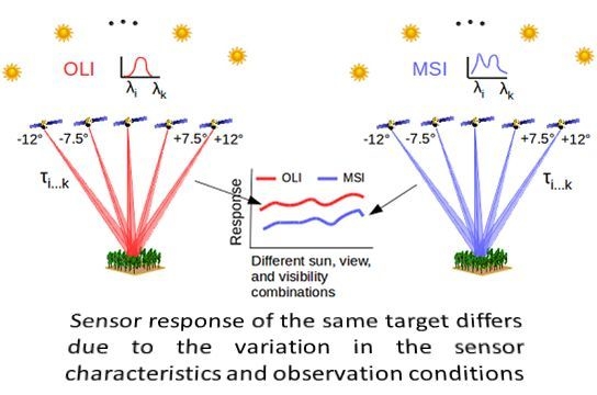
1. Introduction
The ready and free access to moderate resolution remote sensing data from satellites such as Landsat and Sentinel-2 offers the potential to monitor the long (inter-annual) and short term (annual) trends in the condition of the Earth’s resources at finer spatial scales. This is possible not only because of free access to the entire Landsat and Sentinel-2 archive, but also because the data are made available in surface reflectance, thereby allowing more direct comparison of the change in surface condition over time, providing accurate radiometrically and geometrically calibrated products [1,2,3,4].
However, short-term resource monitoring applications require high temporal revisit of the same region of Earth, driving a necessity to collect data approximately once a day. It is expensive and impractical to expect a single mission like Landsat or Sentinel-2 to collect high temporal data without sacrificing the existing requirements for high spatial, spectral, and radiometric fidelity. Although researchers have taken advantage of using multi-sensor datasets to fill the temporal gaps, there is an inherent issue in using more than one sensor’s data due to the differences in the method of measurement, sensor parameters, calibration accuracies, and uncontrollable environmental conditions. The differences in these factors can introduce large variation in the observation, which can complicate the models used in the trend analysis. For example, Reference [5] developed an enhanced TIMESAT algorithm to model and retrieve the vegetation phenology using MODIS NDVI products that showed improved accuracy in the retrieval of phenology metrics in comparison to the original TIMESAT algorithm. The fitted trend using the original and enhanced algorithm suggests that a large variability in the MODIS NDVI observations, even for a very short time duration, are likely due to the uncompensated or residual errors from the radiometric calibrations, atmospheric compensation, and other factors. Such outlier observations are highly likely when more than one sensor is used for time-series analysis. Most of the current research focuses primarily on cross calibrating the data from different sensors by using coincident or near-coincident images over stable pseudo-invariant sites and use of the derived relationship to convert one sensor’s data to the other [6,7]. This still raises a few issues because the target of interest has an anisotropic Bi-directional Reflectance Distribution Function (BRDF), which will be viewed from different illumination and view angles depending on the sensor’s orbital parameters and target’s slope and geographic location. Furthermore, if the two sensors observe the same target on two different dates, changes in the atmospheric conditions can induce additional variations in the data products. Although it may not be possible to compensate for these factors accurately, it is important to understand the magnitude of the factors’ affects to ascertain its impact in time-series, trend models, and change detection studies. The goal of this paper is to demonstrate (a) the potential of a simulation tool in modeling forest defoliation, (b) characterization of canopy defoliation using a simulation environment, (c) the ability to model the relationship between the sources of variation and image-derived measurements, and (d) to provide the magnitude of the factors’ effects. In this work, we used a modeling approach to model and generate the spectral BRDF of a deciduous canopy for different levels of defoliation or Leaf Area Index (LAI), and have used the characterized defoliated forest signal to study the effect of the following four factors that affect the multi-sensor datasets for time-series analysis: (1) Relative Spectral Response (RSR), (2) view angle differences, (3) atmospheric differences, and (4) illumination differences.
Recently, several studies have compared the products from Landsat 8 and Sentinel 2 to characterize and normalize the differences between the two sensors [8,9,10]. While these studies have provided transformation or regression coefficients to generate harmonized data products and have also identified the factors in our study as the source of variation, they do not provide the effect of these factors or their relative magnitude, which is the focus of our study. The inherent issue with these studies is that, the sources of variation cannot be separated or studied independently using the images acquired by these sensors. This limitation does not impact our study because, we implement a modeling approach in a virtual environment to model and understand the complex interaction and the effect of these factors. Secondly, the differences between the data products in the previously mentioned studies are characterized in absolute units such as reflectance, which may not be readily useful for foresters. For example, an uncertainty error of 2% in reflectance on a deciduous canopy is less useful for a forester than to know the uncertainty that would result in the estimation of LAI or forest defoliation when two or more data products are used in the change detection analysis. Our study not only provides the uncertainty estimate in the form of defoliation, but also provides the residual uncertainty when the sources of variation are compensated. Future research in forest applications can make use of these uncertainty estimates to propagate the error from the source to their models, and eventually to their findings. For example, researchers interested in the estimation of LAI, level of defoliation, or biomass can propagate the uncertainties in the remotely sensed data due to calibration, sensor and environmental factors, and the compensation algorithms to their models and thereby can evaluate the error budget associated with their estimates. Although very few studies have used such uncertainty metrics in their application, with the focus and use of big data in remote sensing, many algorithms, models, and applications have to consider the intrinsic and extrinsic characteristics of data, such as our canopy spectral BRDF models, defoliation characterization models, and uncertainty estimates, to provide more useful and accurate information to the scientific community [11,12]. Furthermore, the paradigm shift to the “big data in remote sensing” using Graphic Processing Unit (GPU) programming, cloud computing, and cloud storage supports new applications that rely on simulation environments to model complex phenomenon. For example, the generation of hyperspectral canopy BRDF measurements for different levels of defoliation requires a large number of canopy radiative transfer simulations, which are best solved using cloud computing techniques [13,14]. The simulation process, as outlined in this study can be used as a template for similar studies where ground targets cannot be varied in a controlled setting. For example, BRDF for different land cover types as a function of phenology which are difficult to achieve using conventional methods, can be explored using simulation tools.
This paper is organized as follows. In Section 2, we present the method used to model and characterize forest defoliation for different types of data products. This section also discusses the methods used to analyze the four factors evaluated in this study. In Section 3, we show the results of canopy defoliation and discuss the effect of the different factors. We conclude in Section 4 by providing the uncertainty estimates due to variations in each factor with and without the compensation techniques, and recommendations to the remote sensing community.
2. Materials and Methods
To accomplish the goal of this research, our approach is to simulate the surface, atmosphere, and sensor characteristics, and evaluate the effects of these four factors entirely in a virtual environment so that the limitations with unknowns in the real-data are mitigated. We used a deciduous forest canopy representing the Harvard Hardwood forest [15,16] to model the surface characteristics and the sensor characteristics of Landsat 8 Operational Land Image (OLI) and Sentinel 2 Multi Spectral Instrument (MSI) are used as representatives to simulate remotely sensed data products. The Digital Imaging and Remote Sensing Image Generation (DIRSIG) model, a synthetic image generation tool developed by Rochester Institute of Technology (RIT), is used for simulating the interactions between the sensor, atmosphere and the canopy. The DIRSIG tool has been widely used in many research projects and its capabilities to accurately model the real-world scenes have been validated and compiled in [13,17,18]. The DIRSIG tool was also compared and validated against a wide range of canopy radiative transfer models used in the Radiation Model Intercomparison (RAMI-III) studies and was found to be consistent with the majority of the models such as FLIGHT, DART, Rayspread, etc. [19,20]. Our approach to evaluate the effects of the factors can be summarized in these steps: (1) Model the forest canopy for different levels of defoliation and evaluate the BRDF for each of these varying canopies, (2) Model the sensor and atmospheric characteristics in the DIRSIG tool, (3) Characterize the level of defoliation for different types of data products such as at-sensor radiance, top of atmosphere (TOA) reflectance, surface reflectance, and NDVI, and (4) Vary the factors one at a time and evaluate its effects.
An approach to model the geometry and optical properties of a forest canopy using the DIRSIG tool was presented in [13]. The study further showed that the simulated BRDF, using this approach, was found to agree with the Landsat 8 surface reflectance product to within 2% in both the NIR and red spectral bands. We used the modeled canopy from this study and extended that approach to generate canopies for varying Leaf Area Index (LAI). The biophysical variation of a forest canopy can be represented in many different ways, and we chose to represent the canopy variation in the form of forest defoliation as it severely affects the forest ecosystems, especially when defoliated due to invasive species [21,22]. For completeness and ease of understanding, we describe the forest modeling approach briefly in this section, followed by the method used to generate the defoliated canopy BRDF.
2.1. Forest Canopy Model
A real-world forest canopy consists of trees from a few different species with varying height and Diameter at Breast Height (DBH) over an undulating surface covered with litter from twigs and dried leaves. It is difficult to model an exact replica of a real forest, and hence it is necessary to make a few assumptions on the geometric, spatial, spectral, and optical properties of the tree model to reduce the complexities of the synthetic canopy scene. The synthetic scene was based on real-world Harvard forest data, but the 3D geometry was simplified by using the tree building tool (OnyxTree, Ref. [23]) to model the dominant and co-dominant trees. Although the tree model may not match the actual tree geometry of any specific tree in the Harvard forest, the parameters in OnyxTree were modified such that the LAI of the trees matches the LAI from the forest inventory. Similarly, the trees were placed spatially using the Poisson disc sampling method, which approximates natural placements observed in a homogeneous forest, such that the LAI of the synthetic canopy scene matches the LAI of the actual forest. Using the PROSPECT [24,25] forward/inversion tool, the field collected reflectance spectra were inverted to estimate the transmittance for the leaves. For species, where spectral information was unavailable, spectrally close optical properties were used. Thus, a virtual canopy scene was built that closely matched the real-world optical properties and LAI of the forest.
The radiative transfer within the canopy was estimated by integrating the interaction effects (absorption, reflectance, and transmittance) from a finer scale (facets) for leaves, twigs, branches, trunk and ground to represent canopy level observations using the DIRSIG canopy radiative transfer model. The DIRSIG tool was also used as a virtual goniometer by generating integrated reflectance values for varying spectral, view, and illumination conditions. These BRDF measurements were then fitted to a widely used RossLi canopy BRDF model [26,27] to estimate the model coefficients at finer spatial-spectral resolution in the VIS-NIR-SWIR regions. The advantage of modeling the spectral BRDF of the canopy is that we can generate higher level data products such as NDVI or other vegetation indices easily for any specific view and sun angle geometries.
2.2. Modeling Defoliation
Defoliation refers to the loss of leaves from trees due to the process of senescence or infestation (gypsy moth). In the case of pest infection, the defoliation is rapid and affects the leaf area with minimal to no changes to the leaf’s optical properties. For example, if less than 50 percent of the tree crown is defoliated, most hardwoods will experience only a slight reduction in radial growth and the trees, in general, can withstand one or two consecutive defoliations [28]. Since the health of the trees seldom change due to defoliation by gypsy moth, the defoliated canopies are modeled in this study such that the optical properties of leaves do not change for varying levels of defoliated geometry.
For generating the geometry of the defoliated trees, we randomly select and remove leaf facets while keeping the secondary level branches and twigs intact. Pests that feed on leaves (e.g., chewing insects) can eat an entire leaf, edges of the leaves, chew holes in the centers of leaves, skeletonize the leaves or eat only the upper or lower portion of the leaf [29]. In the majority of these cases, pests eat parts of the leaves, and hence the approach of removing leaf facets rather than an entire leaf is a valid approximation to the actual defoliation observed in forests. The number of leaf facets in a tree can vary anywhere from 50,000 to 350,000 facets and on average has about 125,000 facets. The number of leaf facets removed for each tree model is dependent on the levels of defoliation. For example, for a 20% defoliation, 20% of the facets are randomly selected and removed from each tree model. We retain the spatial position and orientation of the trees within a canopy for all the defoliated forests. Thus, a defoliated canopy changes only in its leaf geometry (number of leaf facets), whereas the number of trees, their position, and the optical properties are unchanged across different levels of defoliation.
As in the case with the forest canopy model, we used the DIRSIG tool as a virtual goniometer to measure the reflectance in different illumination and viewing geometries. These measurements were then fit to the RossLi model [27,30] to estimate the BRDF for each defoliated canopy. The BRDF model for each defoliated canopy provides the capability to compare the canopy reflectance as a function of different levels of defoliation or LAI, as LAI is directly related to defoliation. Modeling a high resolution forest and its defoliation in a simulation environment provides a level of control over different forest canopy attributes such as tree species, their distributions, etc. and provides the ability to estimate the canopy parameters such as LAI directly, at levels of fidelity that cannot be acquired from real-data.
2.3. Modeling the Signal for Different Data Products
The defoliated BRDF provides the ability to compare the reflectance for varying degrees of defoliation. However, in many change detection applications, it is as important to measure the relative change from the reference as absolute differences in radiometric units. Hence, in this study, we used “relative change” (see Equation (1)) as the metric for characterizing the defoliation signal.
Although the levels of defoliation can be measured in units such as LAI in the simulation environment, they cannot be directly measured from the moderate resolution remote sensing data such as Landsat and Sentinel data products. However, LAI of a canopy is typically inferred using regression or other model techniques using field measured and calibrated data products (at-sensor radiance, at-sensor reflectance, surface reflectance, NDVI, etc.). For this reason, we chose to characterize the defoliation signal for different types of data products rather than restricting it to canopy BRDF.
We used the DIRSIG tool to simulate the sensor reaching radiance of the forest canopy scene. The DIRSIG simulation consists of a scene to represent the ground (or BRDF model), a sensor to image the scene, and uses MODerate resolution atmospheric TRANsmission (MODTRAN) to model the atmosphere. In this study, the scene is modeled as a spheroid with the radius of the Earth, and its surface property is modeled using the computed BRDF of the defoliated canopy. The sensor is assumed to fly at L8 altitude and has a single detector with a ground Instantaneous Field of View (IFOV) of 30 m and uses the RSRs of the the OLI and the MSI sensors. The visibility conditions are provided to the MODTRAN [31] tape5 file to simulate the atmospheric attenuations for a mid-latitude summer atmosphere with rural aerosol .
For each defoliated canopy scene, we computed the at-sensor radiance under different sensor and environmental conditions. Table 1 shows the visibility conditions, view and sun angles, and the two RSRs used to estimate the TOA radiance using the DIRSIG tool. We restricted our simulations to the view angles in the across-track direction, as the OLI and MSI have very narrow field of view in the along-track direction (<2°). Similarly, we restricted the sun angles to angles expected during the growing season (Apr-Oct) over the Harvard forest. Typically, red and NIR spectral bands are used for monitoring the changes in the canopy, and therefore all the analysis are performed for these two spectral bands. The total number of simulations from 10 sun angles, 5 view angles, 4 visibility conditions, two RSRs for 9 defoliation levels result in 3600 simulations for each spectral band.
We computed the relative change (see Equation (1)) in TOA radiance for different observation conditions and for each defoliated canopy using the canopy with no defoliation as reference. The mean relative change from these observations indicate the expected change in TOA radiance due to defoliation and the standard deviation represents the deviation due to observation conditions which indicate the validity of the characterization. The estimated mean relative change is devoid of effects due to factors (SZN, VZN, visibility, RSR, etc.) as the relative change is computed between two defoliated forests (or BRDFs) under the same observation conditions. The defoliated forest signal for TOA products is characterized by modeling the expected change in TOA radiance as a function of defoliation levels (or LAI) using least squares fit to linear () and exponential functions (). We initially attempted several models including polynomial-based models, and found that the exponential model performed the best across all levels of defoliation, while a linear model was a good approximation in the NIR spectrum for large LAIs (LAI: >3). Therefore, we decided to show these two models for better comparisons of what to expect from them. To evaluate the accuracy of the model fit, all the models were fitted excluding the 25% defoliation, which is used as validation data to compare the model prediction with the measured estimates. The characterization of defoliation using a functional form provides a way to estimate (interpolate) the level of defoliation for a specific “relative change” in the TOA products. We evaluated the validity of these functions by estimating the difference between the prediction and the actual value for one of the defoliated canopy levels that was not used in modeling the functions. The process to characterize the defoliated signal for other data products are similar, except that the data products are generated differently as described below.
2.3.1. TOA Reflectance Data
A reduction in between-scene variability for clear scenes can be achieved through a normalization for solar irradiance by converting the TOA radiance to TOA reflectance [32]. This type of data typically contains both the surface and atmospheric reflectance of the Earth and is computed as shown in Equation (2). The mean solar exoatmospheric irradiance used for red and NIR spectral bands are 1547 W/m2/µm and 1044 W/m2/µm respectively. The earth-sun distance (d) changes with the day of the year and can be obtained from [32]. The geographic location of the Harvard forest and the L8 and S2 equatorial crossing times are used to estimate the day of the year for each solar angle from Table 1. The estimated day of the year is used to determine the corresponding earth-sun distance from [32]. Although the variation in earth-sun distance is small within the growing season, we still estimated it for each DIRSIG simulations to avoid any errors in the estimation of the signal.
where,
- is the planetary reflectance
- is the spectral radiance at the sensor’s aperture
- d is the earth-sun distance in astronomical units
- is the mean solar exoatmospheric irradiance
- is the solar zenith angle
2.3.2. Surface Refectance Derived Using ELM
The TOA radiance can be converted to surface reflectance using any number of atmospheric compensation techniques [33]. One such technique is to establish a linear relationship between reflectance panels on the ground and their corresponding at-sensor radiance, which is called as Empirical Line Method (ELM) [33]. Knowing the at-sensor radiance, one can then convert it to surface reflectance using a linear regression equation estimated from the panels, formulation of which is shown in Equation (3). Although this technique is simple, assumption that the atmospheric parameters () are constant over the entire region of interest is only valid and true for small regions as in our modeled canopy scene.
where,
- is the mean exoatmospheric irradiance
- is the reflectance factor of the Lambertian panel
- is the upwelled radiance
- is the downwelled radiance
- is the transmittance from the ground to the sensor
- is the solar zenith angle
For our virtual scene, we placed two Lambertian panels of known reflectance on the ground and simulated their corresponding at-sensor radiance across all observation conditions as shown in Table 1. Typically, an entire real image is compensated for atmospheric effects by imaging calibrated panels at the same time of image acquisition to avoid any effects due to atmospheric and solar angle differences. However, this can introduce errors as the path length of transmission changes for non-nadir view angles. Therefore, in this study, we employ two different methods of ELM, ELM (typical) and ELM (ideal). In the ELM (typical) method, all view angle observations are compensated by the same regression parameters estimated from nadir observed panels, i.e., insensitive to view angle differences as seen in typical atmospheric compensations. In the ELM (ideal) method, each simulated TOA radiance for different observation conditions is compensated by a unique set of regression parameters based on the corresponding panel observations, and therefore, this method will provide an ideal compensation for the atmospheric attenuations.
2.3.3. Surface Refectance from Canopy BRDF
The surface reflectance for a specific sun and view angle can be calculated directly from the DIRSIG generated defoliated canopy BRDF model. For each defoliated canopy, we computed the reflectance for 50 possible observation conditions (10 sun × 5 view = 50 BRDF) using the canopy BRDF model and the sun/view angles shown in Table 1, which represents the typical illumination and view angles expected during the growing season over the Harvard forest for the L8 and S2 sensors. For each defoliated canopy, reflectance observations of the undefoliated canopy (0% defoliation) were used as “reference” (see Equation (1)) to compute the corresponding relative change for the 50 observation conditions, which were then averaged to estimate the mean relative change.
Thus, we have characterized the defoliation as a function of TOA radiance, TOA reflectance, and surface reflectance data products. Many applications rely on the NDVI data for the assessment of forest canopy cover, defoliation, and biomass studies, and therefore, we characterized the defoliation as a function of NDVI using these data products. It is nearly impossible to characterize the expected change from real sensor data, because, the range of forest defoliation needs to be controlled, properly assessed, and the BRDF for these levels of defoliation needs to be accurately measured. This is why a simulation environment is necessary where these variables can be controlled and analyzed independently.
2.4. Factor Effects
By characterizing the relative change in different types of products as a function of defoliation, the detection of signal in the presence of noise (effects due to the sensor and environmental factors) can be studied. The main objective of this study is to estimate the effect of these factors when there are no changes on the ground, for which we have coined the term “Noise Equivalent Defoliation (NED)”. NED is defined as the amount of defoliation that is contributed due to a specific factor. In other words, the effect due to a specific factor is equivalent to the effect that would be observed when the forest defoliates by a certain amount in the absence of noise. By using defoliation as the basis, we have directly related the effect of these factors to actual changes on the ground. The NED is a useful term in understanding the sensitivity of various factors as it indicates the uncertainty in measuring the actual changes in the canopy using remotely sensed products.
In this section, we discuss the methods used to analyze the effect of different sensor and environment factors. While many factors such as slope of the terrain, aerosol differences in the atmosphere, cloud contamination, detector’s responsivity, mis-registration, etc. affect the measured radiance, in this study, we focus on four dominant factors: RSR, across-track view angle, visibility, and solar zenith angle. We found the solar azimuth and along track angles for L8 and S2 were insignificant [14], and mis-registration between the products can be reduced by better calibration and co-registration. The atmospheric effects due to different parameters such as aerosol, cloud contamination, etc. are complex and difficult to model. Hence, we chose a single variable (visibility) with fixed MODTRAN parameters (rural aerosol, mid-latitude summer, etc.) to represent the attenuations expected due to atmospheric differences between the two products. The slope of the terrain does impact the at-sensor radiance, but for time series analysis, where the same pixel on the ground is observed by two or more sensors, the terrain does not have a direct impact. However, two or more sensors observing the same ground pixel from different view angles can affect the at-sensor radiance, but most of this is captured by the effect in the across-track angles. Since it is impossible to control these factors with the real data, we used the simulated data to perform this sensitivity analysis.
2.4.1. RSR
The RSR for OLI (L8) and MSI (S2A) sensors are found in several literatures [34,35,36,37]. In this study, we used the narrow band NIR (Band 8a) and red (Band 4) spectral bands of the Sentinel 2A response functions. Please note that a new update for the spectral response functions of Sentinel 2A was published recently, but when compared with the previous issue (2.0), the new version updates mainly changes the responses for blue and coastal aerosol bands (Bands 1 and 2 ) [8,38] and therefore, the RSRs used in this study for NIR and red bands are consistent with the updated RSRs. The center wavelength and the shape of the RSR are similar between OLI and MSI sensors in the NIR spectral band, but are dissimilar in the red band. When the data from these two sensors are used in time-series analysis, the differences in RSR are likely to produce different responses while observing the same target. By modeling these RSRs in DIRSIG, we attempt to estimate the expected differences in different data products solely due to RSR dissimilarities. To estimate the effect of RSR, we have simulated the at-sensor radiance under different visibility conditions, across-track angles, and sun angles to represent the acquisition on different days of the year, atmospheric conditions, and viewing the target from different view angles. Figure 1 shows a pictorial representation of the simulation combinations. The ten sun angles, five view angles, and the four visibility conditions used in the simulations (200 observations) are listed in Table 1 for the two RSRs (OLI, MSI) in the red and NIR spectral bands. The mean relative change in response to different types of simulated NDVI data products from these observations and the characterized defoliation signal (exponential function) are used to estimate the effect of RSR in NED units. The relative changes between the two sensors are calculated for the same observation condition, therefore, the change measured is due to the differences in RSR alone and is not affected by other factors. We also estimated the effect of RSR for different signal levels (defoliated BRDFs) and found that the effect was independent of the signal level.
Research has shown that the effect due to RSR could be mitigated using Spectral Band Adjustment Factor (SBAF) techniques [39,40,41]. In our study, we applied two SBAF techniques to evaluate the residual effect after compensation. In the first SBAF technique, a scale factor is determined between the two sensor observations without using the shape of RSR [40]. The second technique uses the TOA reflectance of the target from hyperspectral data and the shape of the two RSRs to estimate the SBAF [39]. Both the methods suffer from the BRDF effects of the target and atmospheric differences between the two datasets. In our study, we generated two SBAFs: (1) using the first method for TOA reflectance data, and (2) using the second method with modeled canopy BRDF instead of TOA reflectance, thereby avoiding any atmospheric and BRDF effects. Equation (4) shows the formulation for SBAF computation. For the first SBAF method, we chose 100 randomly selected TOA observations from Table 1 to derive the SBAF while the second method uses 72 sun and view angle combinations to estimate the SBAF.
where,
- is the TOA reflectance for a specific spectral band
- is the effective BRDF reflectance (adjusted by the shape of the RSR)
- is the BRDF reflectance of the canopy
- n is the number of sun, view , and visibility combinations randomly selected
- k is the number of sun, view combinations shown in Table 1
2.4.2. Across-Track View Angle Effects
The two sensors seldom view a ground target with the same view angle, as their orbital parameters and fields of view are different. The view angle difference between the two sensors to a target is dependent on the geographic location of the target. In some cases, imaging the same ground target by one sensor in the backscatter direction and the other in the forward scatter direction can result in differences as high as 30% in reflectance for canopies in the NIR spectral bands, even for a near coincident imaging. Therefore, it is necessary to estimate the effect due to view angle differences, which is dependent on the BRDF of the target.
Similar to RSR, we estimated the effect due to view angle differences for the two sensors from the simulated responses for ten sun angles, four visibility conditions and the characterized defoliated signal. The mean relative change across different view angle combinations between the two sensors result in an effect that is due to the differences in both the view angle and the RSR. We intentionally estimated this, as the real data from two or more sensors inherently exhibit this coupled effect. The effect only due to across-track view angle difference was also estimated for a unique case with two extreme view angles (±12°) by combining the simulated responses from the two sensors. As in the case with the RSR, we estimated the effect due to view angle differences for the different NDVI data products, both with and without the compensation for the RSR differences.
2.4.3. Visibility
Because the L8 and S2 sensors operate from different orbits, coincident imaging is not possible for most regions on the Earth. Even for regions where near-coincident imaging is possible, the time of acquisition still vary by about 20 min due to differences in the equatorial crossing time. Since the two sensors are less likely to image on the same day and time, any differences in the atmospheric conditions can introduce a large variation in the sensor reaching radiance and therefore it is important to estimate this effect. The effect is dependent on the severity of the differences in the atmospheric conditions and therefore, in this study, we simulated the effect for dissimilar visibility conditions. Using the responses of the two sensors observing the same ground scene under different visibility conditions averaged over ten sun angles and five view angles, we estimated the mean relative change and its corresponding effect in NED units. Although this provides the effect due to visibility differences, the estimated effect also includes the effect due to RSR differences. As in the case of view angle effect, we estimated the effect of atmospheric differences devoid of RSR for the different NDVI data products by averaging the simulated responses under different atmospheric conditions.
2.4.4. Solar Zenith (SZN) Effect
Typically, the two sensors acquire images of the same target on two different days and time, which not only affects the atmospheric conditions, but also the solar zenith angle. For example, two images acquired within a span of 1 hour in June over Harvard forest can differ by as much as 10 degrees in SZN. Due to the azimuthal symmetricity assumption for the forest canopies, any effect due to solar azimuth angle can be ignored, but the solar zenith angle introduces a direct cosine effect in the TOA radiance. The SZN effect is dependent on the magnitude of the difference in the SZN angles, the time of the year (seasons), and the geographic location of the forest. Using the Harvard forest’s geographic location, we found that the SZN angle for the two sensors acquisition can vary anywhere between 2 to 5 degrees for same day acquisition and can be as high as 10 degrees for day offset by 20 days. Therefore, for the SZN effect estimation, we generated two sets of simulations for different view angles, RSR and atmospheric conditions: (1) for SZN difference of 5 degrees and (2) for SZN difference of 10 degrees. Unlike the visibility or view angle effects, the effect estimated in this case is independent of any other factor’s effects as the relative change is averaged over similar observation conditions except for the difference in SZN angles. In general, change detection applications use TOA reflectance or surface reflectance products for their analysis, and thereby avoid the majority of the effects due to SZN differences. However, the differences in the illumination geometry can introduce residual effects due to the BRDF of the forest canopy, which we can infer from the effect in the reflectance-based NDVI products.
3. Results and Discussion
3.1. Defoliated Forests
The modeling of defoliated canopies in DIRSIG is useful in approximating the natural process and for studies to understand the relationship between biophysical parameters and BRDF. In this study, the BRDFs generated for the defoliated forests are used to characterize and evaluate the effect of sensor and environmental factors. Figure 2 shows the simulated RGB image for six of the nine defoliated forests demonstrating the variation for different levels of defoliation. The visual image does not show any remarkable differences even at 40% defoliation because, the LAI of the forest even at 40% is about 3, which in general is high, and secondly, the leaf facets and not the entire leaves were randomly removed, and lastly, the twigs and branches along with the leaf facets make the image look cluttered. To ensure that the modeling of defoliated forest is reasonably accurate, we computed the LAI of each defoliated forest directly from the geometry of the leaf facets and compared it against the level of defoliation. The relative change in LAI computed as ( is the LAI when there is no defoliation and refers to the LAI at different levels of defoliation), matches one-to-one with the levels of defoliation as expected (see Figure 3).
From Figure 4 , it is observed that the reflectance for different levels of defoliation can vary anywhere between 0.2 to 0.4 in the nadir view for NIR band and much higher in the back-scattered direction, while the reflectance in general is very low in the red spectral band and varies between 0.01 to 0.03. The hot-spot effect is observed in the principal plane at the back-scatter direction for all the defoliated levels. The high NIR reflectance and low red reflectance is mainly due to the multiple scattering (transmittance and reflectance) of leaves in the NIR region, and also, the field measured leaf optical properties were for healthy green leaves during peak growing season. It is also evident from the figure that the red reflectance increases with increase in defoliation while the NIR reflectance reduces due to the reduction in NIR scattering. In general, the bi-directional reflectance vary anywhere between 5% to 60% in the NIR band and even higher in the red band, depending on the level of defoliation. It is interesting to note that the rate of increase or decrease in the reflectance for corresponding reduction in LAI in the principal or cross plane is not linear. This suggest that the studies that rely on reflectance measurement to detect the onset of defoliation require high precision sensors that can detect small changes in reflectance.
3.2. Modeling the Signal for Different Products
3.2.1. Radiance and Reflectance Products
The method used to simulate the TOA radiance, its conversion to TOA and surface reflectance, and the characterization of defoliation for these data products was discussed in Section 2.3. Table 2 and Table 3 show the mean relative change and its standard deviation for different levels of defoliation for products that are uncorrected (TOA RAD), corrected for planetary reflectance (TOA REFL), compensated for atmospheric attenuations (ELM-ideal, ELM-typical), and modeled surface reflectance (BRF) in the red and NIR spectral bands respectively. The mean relative change is used to characterize defoliation by fitting an exponential curve of the form , as shown in Figure 5, Figure 6 and Figure 7 for TOA radiance, ELM-ideal, ELM-typical, and surface reflectance (BRF) products. The standard deviation (STD) is shown as error-bars in these plots. It is observed from these plots that the relative change increases with an increase in defoliation in the red and NIR spectral bands due to the increase in the red reflectance and reduction in the NIR reflectance. Please note that the relative change is a measure of the absolute difference with respect to the reference, and therefore, both the NIR and red spectral bands show an increase in relative change. Furthermore, it is evident from these figures that the exponential function characterizes the defoliated signal better than the linear function, which is the case for all the other data products (Figure 8).
From the Table 2 and Table 3, we find that the TOA REFL and TOA RAD products are identical as the TOA reflectance varies from the TOA radiance by a scale factor (adjustment for SZN angle, irradiance), which is essentially negated when the relative change is computed. The relative change for TOA products is significantly lower than the atmospheric compensated products, which suggests that the atmospheric attenuations function as blur or low pass filter and reduces the actual variability on the ground. This feature is more prominent in the red band as the scattering of the atmosphere is higher in the red band than the NIR band. This further suggests that the variability on the ground can be better assessed using surface reflectance products than TOA products. While this is true, it is important to note that the STD is also higher for the surface reflectance products than TOA products in the red band, which indicates that the differences in the observation conditions can introduce large variability, if their effects are not corrected. This effect is also observed when the residual error in the atmospheric compensation or other correction algorithm is high as in the case of ELM-typical products, which show higher STD than ELM-ideal or BRF products. Please note that the ELM-typical method does not account for the change in transmittance due to the differences in the view angle, which introduces larger variability in the atmospheric compensated products. For surface reflectance products (ELM-ideal and BRF), the main contributor to the STD is the variation in the illumination and view geometries.
In the case of NIR band, the STD in the surface reflectance products are lower than the TOA products, which suggests that effect due to differences in the observation conditions are relatively small. These are explored in more detail in Section 3.3. Between ELM-ideal and ELM-typical, the STD is similar as the atmospheric attenuation is considerably lower in the NIR, resulting in negligible differences between the two atmospheric compensation techniques. The defoliation characterization between the ELM-ideal and the one directly based on the canopy BRDF model (BRF) is almost identical (see Table 3, Figure 6 and Figure 7), further suggesting that a simple technique like ELM with exact view geometry has the potential to perform an accurate atmospheric compensation. The main drawback with this method is that it is impractical to deploy panels across the entire scene, time-consuming, and expensive to use the panels for generating surface reflectance products for real-world datasets. However, this technique can be very useful and is being used for calibrating and validating the atmospherically compensated products [42]. From this study, we find that a deciduous forest canopy that defoliates by 30% can induce a change as high as 10% in the surface reflectance of NIR band.
3.2.2. NDVI Products
We characterized the defoliation for different types of NDVI products using the calculated TOA radiance, TOA reflectance, and surface reflectance (ELM-ideal, ELM-typical, and BRF) for the red and NIR bands (see Table 4 and Figure 8). As expected, the characteristics such as STD for the NDVI products are similar to that of the TOA and surface reflectance products as discussed earlier. However, for the NDVI products, the TOA REFL products are not identical to TOA RAD products. This is because, the irradiance in the red and NIR spectral bands are different, and therefore, the calculated NDVI is also different between the TOA RAD and TOA REFL products. In all these characterization, the STD is less than 10% of the mean, indicating that the relative change-based characterization is a useful metric to estimate the effects of the factors.
Interestingly, the plot of NDVI for different types of NDVI products (see Figure 9) indicate that the canopy NDVI value and its trend is dependent on the compensation techniques used to generate the NDVI products. Therefore, it is important to remember that the NDVI values of a canopy estimated from one type of data product should not be combined with the NDVI product from a different source without proper normalization. In general, the NDVI is assumed to vary linearly with LAI for sparse canopies with low LAI (ranging from 1 to 3) [43], but from this study, it is observed that the relationship between NDVI and LAI may be better approximated by an exponential function over the full range of canopy densities.
In this study, we estimated the fit accuracy of the exponential function for all the characterized curves using one of the defoliation levels as a validation point (defoliation = 25%). We compared both the linear and exponential models for all these characterized functions for the validation point, and found that the linear model introduces an error that is significantly higher than 90% for most of the data products, essentially making it undesirable to characterize defoliation signal. From Figure 5, Figure 6, Figure 7 and Figure 8, it is observed that the exponential model performs significantly better than the linear models for the validation point. The fit accuracy shown in Table 5 for the exponential model suggests that the exponential curve can estimate the defoliation from the relative change to within 10% relative error for the NDVI products and to within 2% for the NIR products. The higher error estimate for the NDVI products is mainly due to the low reflectance of the canopy (1% to 3%) in the red band. Although the validation error is seemingly large (10%), it introduces an error no greater than 2.5% in defoliation estimation for a 25% defoliated canopy.
3.3. Factor Effect Analysis
We analyzed the effect of the four factors by varying one factor at a time, while keeping all the other factors at a constant level. The results for each of the factors are shown below.
3.3.1. RSR
The two sensors have different spectral responses (RSR), especially in the red band, which affects the derived products such as NDVI. For the NDVI products, the relative change is estimated by observing the differences under the same view, illumination and visibility conditions. Although this is a hypothetical situation, as the expectation that the two sensors image the target on the same day and time is highly unlikely, it still stands useful to understand the effects with and without the compensation for the spectral response differences for the different NDVI products.
The SBAF techniques described earlier is used to compensate for the spectral differences in the TOA and surface reflectance measurements, which are used to calculate the NDVI. In this study, we used 200 simulated TOA observations (10 sun, 5 view, 4 visibility) to estimate the mean relative change, which are then converted to NED units using the characterized exponential function for all the NDVI products. Table 6 shows the effect of the RSR differences for the compensated and uncompensated NDVI products. It is observed that the effect of RSR is dependent on the level of compensation, and in the TOA products, the effect of RSR can be as high as 20% in NED. This suggests that the estimated changes on the ground has an uncertainty of 20% due to the RSR differences if the two sensors are used directly in change detection applications. However, if the data are compensated using SBAF techniques, the uncertainty can be reduced to about 1% in the change detection applications. Interestingly, the uncertainty for SBAF compensated products is dependent on the type of method used for compensation and the type of products. For TOA reflectance products, the SBAF method using the TOA reflectance has lower uncertainty than for the surface reflectance products, while the effect is vice versa for the SBAF method using BRF. This clearly suggests that the SBAF derived method should be consistent with the type of data products used in the remote sensing applications.
3.3.2. Across-Track effect
We analyzed the across track effects for two scenarios; (1) when the across track angles are different for two sensors, (2) for the two extreme angles for the same sensors. The first scenario directly relates to the effect due to both the RSR and the across-track angles, a typical situation encountered when using the two sensor products for change detection. The second case directly relates to the case when two Sentinel-2 or other sensors with similar field of view viewing the same target from two extreme view angles (±12°). Although it is unlikely for OLI sensor due to its narrow field of view (±7.5°), nevertheless, these conditions are useful for future Landsat or any other sensors with larger FOV. The mean effect in NED shown in Table 7 is calculated by averaging the relative change across different view angle combinations (L8/S2: 7.5°/12°, 7.5°/0°, 0°/7.5°, 0°/12°, −7.5°/−12°, −7.5°/0°, 0°/−7.5°, 0°/−12°, 7.5°/−7.5°, −7.5°/7.5°, 7.5°/−12°, 7.5°/12°). The STD in the table is mainly due to the large variation in the effects for the different view angle combinations. The effects estimated for the two extreme angles shown in Table 8 does not include any contribution due to the RSR differences, and the STD is attributed to the BRDF of the canopy and variations due to the visibility and illumination conditions. The high STD for the surface reflectance-based NDVI products suggests that the main contributor to the variation is due to the BRDF effects of the canopy.
For the ELM-ideal products, reflectance panels are used to correct for every view angle independently and therefore the effects are similar to that of the BRF-based products. The ELM-typical NDVI products show larger effects than any other products, mainly due to the residual error in the atmospheric compensation technique. Because the ELM-typical products compensate based on the nadir panel observations, the red reflectance in the back-scatter direction (−12°) is over estimated due to the difference in the path-transmission and increase in the upwelled radiance. In the NIR band, the difference in transmission between nadir and non-nadir view is small, and so the reflectance estimated in NIR is unaffected. Over-estimation of red reflectance results in the under estimation of the NDVI score. However in the forward scatter direction, the red reflectance changes only marginally and the NIR reflectance is unaffected as before, leading to smaller effects.
We see that the SBAF compensation reduces the effect of view angles on an average to 8% to 10% uncertainty for the TOA products, whereas, for the ideal surface reflectance products, the effect is reduced further to 5%. In such cases, when there is residual error in the atmospheric compensation, which is highly likely in most of the atmospheric compensated products, the effect due to the view angle could be as high as 28% in NED between OLI and MSI sensors even after SBAF correction. For extreme view angles (±12°), the effect increases further to about 40% with a very high STD (22%), which is mainly due to the variation in the atmospheric conditions. The coupled effect of residual error in atmospheric compensation and the view angle differences can introduce large uncertainty for change detections.
3.3.3. Visibility Effects
The effect due to the differences in the atmospheric conditions is simulated by varying the visibility conditions for mid-latitude summer atmosphere with rural aerosol. For these simulations, the two sensors (OLI and MSI) view the target from the same view and illumination angles, but under different visibility conditions, as in the case with real sensor data, when the two sensors image on two different dates with different atmospheric conditions. Although the illumination and view angle may also differ, the view angle difference is dependent on the geographic location of the target while the illumination angle depends on the time difference between the two acquisitions. The effect estimated in this case is due to the combined effect of differences in visibility conditions and the RSR between the two sensors. As in the case for view angle, we estimated the effect with and without the SBAF correction as shown in Table 9.
The large variability (STD) is due to the varying visibility combinations between the two sensors, and the effect increases with increase in the visibility differences. For example, the effect increases as the visibility of S2 varies from 20 KM to 10 KM for the fixed visibility of 20 KM for L8. This is expected as the visibility is directly proportional to transmission, and so a larger ΔVIS causes larger differences in the transmission, resulting in a higher estimate in NED. Similarly, for the same difference in visibility between the two sensors, the effect estimate is high when the visibility is low and this is because, the optical depth is not linear but exponentially related to visibility. For example, the estimated effect in visibility between 15 KM (L8), and 10 KM (S2) is higher than the effect between 20 KM (L8) and 15 KM (S2), although the ΔVIS for both the cases are same (5 KM).
As expected, the effect is about 40% for the TOA products, as they are uncompensated for atmospheric attenuations. The effect did not vary despite the SBAF correction, as the contribution of RSR differences is insignificant compared to the contribution due to the differences in the visibility conditions of the atmosphere. In the case of atmospheric compensated products, the effect is about 15%, but when compensated for the RSR differences, the effect reduces to 8% to 1% depending on the type of compensation method for RSR and atmosphere. Because the ELM-typical method does not account for off-nadir path length differences, its effect is higher than that of ELM-ideal product. The STD for the ELM-typical method is large for the SBAF adjusted products, suggesting that the effect or the uncertainty in change detection application is dependent on both the inaccuracies of the atmospheric compensation method as well as the condition of the atmosphere. Thus in a situation where both the sun and view geometries are the same, and the RSR and atmospheric differences are accurately compensated, the residual effect can be reduced to 1% in NED, i.e., the changes on the ground can be ascertained to within 1% uncertainty. In practice, it is difficult to achieve an ideal compensation for the atmosphere, and the sun and view geometries are less likely to be similar between the two acquisitions, and therefore, it is not unreasonable to expect an uncertainty of about 10% in the change detection applications using the atmospheric compensated NDVI products.
3.3.4. SZN Effects
The L8 (OLI sensor) has a revisit period of 10 days and the S2 sensors (2A and 2B) each have a revisit period of 10 days, but when combined achieve a 5 days revisit period. The Landsat and Sentinel sensors can image the target to within 10 days, but operational issues in acquiring the target or presence of clouds over the target can potentially increase this duration. Therefore, we estimated the possible differences in SZN angles between L8 and S2 based on their orbital parameters over the Harvard forest, assuming that the two sensors image the target within 20 days. The estimated absolute difference in SZN angle varies from 2 degrees to 4.5 degrees for 5 days difference between L8 and S2, and about 8 degrees when they are 20 days apart during the growing season. Figure 10 shows the plot of SZN difference for an entire year over the Harvard forest, which is estimated based on the nominal equatorial crossing time of the two sensors. Since this difference is dependent on the geographical location, similar analysis over the Amazon forest (equator) showed that the SZN difference range between 5 to 7 degrees for 5 days difference for these two sensors. The difference in SZN angle tends to decrease as we move away from the equator. Therefore, in our study, we estimated the effects for the two cases: (1) when SZN difference is 5 degrees and (2) when SZN difference is 10 degrees. In our simulations, we chose the SZN angles for Landsat 8 that are expected over the Harvard forest, and adjusted the SZN by about 5 and 10 degrees for the Sentinel 2 sensors, ensuring that the chosen SZN angles are within the expected range for the Sentinel 2 over the Harvard forest.
As with the other factors, the simulated TOA and surface reflectance-based NDVI products are used to estimate the effects of SZN in NED units. For these simulations, the atmospheric conditions and the view angles are assumed to be the same, while the SZN angle is varied by about 5 degrees and 10 degrees. The effect due to SZN, as shown in Table 10, is estimated for each sensor independently and averaged together to avoid any additional increase due to RSR differences. Thus, in a situation where two sensors with similar RSRs image the target at the same view angle and atmospheric conditions, then the effect due to SZN is about 10% in NED for a ΔSZN of 5 degrees. If the data are compensated for the atmospheric attenuations, then the effect varies between 4–8% depending on the accuracy of the compensation technique. Similar analysis for ΔSZN of 10 degrees suggests that the effect doubles for twice the ΔSZN. A key thing to note is that the effect for TOA radiance and TOA reflectance products are identical because the cosine correction for SZN in the TOA reflectance product is essentially negated when the ratio of the bands are computed for NDVI products. In addition, the SBAF correction produces identical effect to that of the uncompensated products because the effects are estimated independently for each sensor, and therefore are devoid of RSR effect. In an ideal condition, when the atmospheric compensation is accurate, any change on the ground can be ascertained to within 4% uncertainty if a sensor images the target on the ground to within 5 degrees difference in SZN angle, and the uncertainty increases linearly with the difference in SZN angle. In practice, it is difficult to achieve an ideal compensation and acquisition conditions, and therefore, the expected uncertainty in the change detection studies will be higher than 4%.
4. Conclusions
In this paper, we illustrated the advantage of using a virtual environment for modeling the biophysical characteristics of a forest and how it can be extended to study the effect of sensor and environmental factors that affect the remotely sensed data.
This paper discusses the in-canopy radiative approach and the impact of defoliation on the reflectance and radiance observed by sensors such as Landsat. We modeled deciduous forests with different LAI (or defoliation) by randomly removing the leaf facets of the 3D modeled trees for different levels of defoliation. Our results indicate that the reflectance for the defoliated forests in the principal and cross planes can introduce differences ranging between 2% to 60% depending on the level of defoliation (10–85%) in the red and NIR spectral bands when compared with the undefoliated canopy. For example, the relative change in forest reflectance between a non-defoliated and 30% defoliated deciduous canopy can be as high as 10% in NIR spectral band. Since many applications rely on detecting defoliation using change detection methods from satellite data, we characterized the canopy defoliation for different satellite data products which includes TOA radiance, TOA reflectance, surface reflectance, and NDVI products. From this study, we conclude that the variation in defoliation of the deciduous canopy and the relative change observed in the remotely sensed data products can be modeled using an exponential function of the form for the red and NIR spectral bands. The coefficients of this functional form varies for the different types of products, but the model fit accuracy is high and consistent across all the data products. The predictive error from this characterization was observed to be 6% and 2% in the red and NIR bands respectively, which relates to an error of about 0.5–1.5% for a 25% defoliated canopy.
In addition to the characterization of defoliation for different sensor products, we also performed a sensitivity study to assess the effect of major factors that affect the change detection analysis when data from one or more sensors are used. The study analyzed the four factors (RSR, cross-track view angle, Visibility, and solar zenith angle) one at a time, and evaluated the effects in Noise Equivalent Defoliation units, which is defined as the amount of defoliation that is contributed by a factor when there is no change in the canopy. Using this unit makes the results of this study easier to understand, as it directly relates to the expected uncertainty due to the effect of the sensor and environmental factors. In our study, we simulated the at-sensor radiance of the modeled canopy BRDF for the OLI (L8) and MSI (S2) sensors using the MODTRAN atmosphere and applied compensation algorithms such as atmospheric compensation techniques (ELM) and SBAF to demonstrate the improvements gained in the uncertainty estimates when such techniques are used. The results and finding from this sensitivity study indicate the following:
- The effect of atmospheric differences between two scenes due to changes in the visibility conditions can introduce as much effect as would be observed when the forest defoliates by 40%, but if compensated, the effect can be reduced to 1–7% in defoliation depending on the accuracy of the atmospheric compensation algorithm. The atmospheric attenuation is observed to be the most significant factor among all the factors considered in this study. Both the USGS (Landsat) and ESA (Sentinel-2) provide TOA products as their default/standard products, and as demonstrated in this study, if the atmosphere is not compensated, the effect of atmosphere can introduce large uncertainty in the estimation of forest defoliation.
- The effect due to RSR differences between Landsat 8 and Sentinel 2 is observed to be 20% in defoliation, but compensation algorithm such as SBAF can reduce the effect to 1–7% in defoliation depending on whether the atmospheric attenuations are compensated or not.
- The cross-track view angle differences can introduce effects anywhere from 9% to 40% in defoliation depending on the accuracy of the atmospheric compensation algorithms.
- For 5 days difference in acquisition between Landsat 8 and Sentinel 2 sensors, the effect of SZN angle differences can introduce effects ranging from 4% to 10% in defoliation depending on whether the atmospheric attenuations are compensated or not.
- Analysis of effects on the real data (OLI) acquired over a period of 23 days indicates that more than half the observed changes are likely to be due to the effects of the factors.
Our study finds that atmospheric compensation is necessary for time-series and change detection applications that attempt to estimate the biophysical parameters from remote sensing data. If data from more than one sensor is used, then the atmospheric compensation algorithm should be accurate, as imperfect compensation is likely to inflate or exaggerate the actual changes on the ground. In addition, the differences in the RSR between the sensors should be compensated, and SBAF techniques as demonstrated in this paper can be useful. The differences in the view angles in the across track direction does impact the changes measured on the ground, but can be reduced using accurate atmospheric compensation algorithms. Because the BRDF is a function of view and illumination angles, view angle differences cannot be compensated completely without the knowledge of the BRDF of the surface. Similarly, the differences in solar zenith angle between the acquisitions can affect the changes measured even when compensated for the atmospheric attenuations, but its effect is dependent on the BRDF of the surface, difference in the time/day between acquisitions, and the geographic location of the biome. Most of the natural surfaces can be approximated as azimuthally symmetric surfaces, and hence the effect due to the solar azimuth angle differences can be ignored for most of the biomes. The effect in the along track direction for the Landsat 8 and Sentinel 2 sensors is negligible and can be ignored. We would like to make the following recommendations to the remote sensing community, especially when multi-temporal and multi-sensor datasets are used in the applications.
- Target specific and sensor specific SBAF values should be estimated and provided to the user community either using the real or simulated data. Many recent studies have used SBAF techniques to normalize for spectral response differences [44,45], but they were predominantly estimated using pseudo-invariant sites like desert sites for calibration purposes. Since SBAF values are both target and sensor specific, modeling approach as shown here for deciduous canopy can be used to estimate for other land cover classes.
- Understanding that the factors identified in this research can introduce real effects, future time series analysis should provide the uncertainty in their estimation that are based on the uncompensated and residual effects. Our study provides the first-order uncertainty estimates due to these factors, which can be used effectively to derive accuracy metrics in forest applications.
- Atmospheric compensation and compensation for sensor differences (RSR) should be applied for the data used in time-series applications. The Landsat and Sentinel-2 data providers have been providing surface reflectance data on-demand, but no associated uncertainty estimates are available for these products. The atmospheric compensation algorithm proposed by [46] and used in generating Landsat surface reflectance products indicate, that it is not uncommon to expect a 6% uncertainty in surface reflectance products using their algorithm. However, this is an overall estimate, and cannot be used as per-pixel uncertainty estimates for every data products. In the future, data providers should focus on per-pixel uncertainty estimates rather than a product or algorithm level uncertainty.
- Future research should focus on validating the accuracy of the atmospheric compensation algorithms used in generating the Landsat surface reflectance products using the real data if possible, or with the simulated data, and improve the algorithm as necessary. As shown in this study, atmospheric compensation has the potential to reduce the uncertainty in the products, but it has to be done correctly, as otherwise, it increases the uncertainty. This is one reason future research should focus on validating the surface reflectance products.
Author Contributions
Conceptualization, J.R.S.; Data curation, R.R.; Formal analysis, R.R.; Funding acquisition, J.R.S.; Investigation, R.R.; Methodology, R.R.; Supervision, J.R.S.; Validation, R.R.; Visualization, R.R.; Writing—Original draft, R.R.; Writing—Review & editing, J.R.S.
Funding
This research was funded by NASA grant number NNX13AQ73.
Acknowledgments
The authors would like to thank Adam A. Goodenough and Scott Brown for their help in developing the canopy radiative transfer model in DIRSIG. We also would like to thank the research teams from University of Massachusetts and Boston University, for sharing their field collected forest inventory and spectral information with us.
Conflicts of Interest
The authors declare no conflict of interest.
References
- Markham, B.L.; Helder, D.L. Forty-year calibrated record of earth-reflected radiance from Landsat: A review. Remote Sens. Environ. 2012, 122, 30–40. [Google Scholar] [CrossRef] [Green Version]
- Schott, J.R.; Gerace, A.D.; Brown, S.D.; Gartley, M.G. Modeling the image performance of the Landsat Data Continuity Mission sensors. In Proceedings of the SPIE Optical Engineering+ Applications, San Diego, CA, USA, 21–25 August 2011; p. 81530F. [Google Scholar]
- Storey, J.C. Landsat 7 on-orbit modulation transfer function estimation. In Proceedings of the International Symposium on Remote Sensing, Toulouse, France, 17–21 September 2001; pp. 50–61. [Google Scholar]
- Masek, J.G.; Vermote, E.F.; Saleous, N.E.; Wolfe, R.; Hall, F.G.; Huemmrich, K.F.; Gao, F.; Kutler, J.; Lim, T.K. A Landsat surface reflectance dataset for North America, 1990–2000. IEEE Geosci. Remote Sens. Lett. 2006, 3, 68–72. [Google Scholar] [CrossRef]
- Tan, B.; Morisette, J.T.; Wolfe, R.E.; Gao, F.; Ederer, G.A.; Nightingale, J.; Pedelty, J.A. An Enhanced TIMESAT Algorithm for Estimating Vegetation Phenology Metrics From MODIS Data. IEEE J. Sel. Top. Appl. Earth Obs. Remote Sens. 2011, 2, 361–371. [Google Scholar] [CrossRef]
- Mishra, N.; Haque, M.O.; Leigh, L.; Aaron, D.; Helder, D.; Markham, B. Radiometric Cross Calibration of Landsat 8 Operational Land Imager (OLI) and Landsat 7 Enhanced Thematic Mapper Plus (ETM+). Remote Sens. 2014, 6, 12619–12638. [Google Scholar] [CrossRef] [Green Version]
- Chander, G.; Meyer, D.J.; Helder, D.L. Cross calibration of the Landsat-7 ETM+ and EO-1 ALI sensor. IEEE Trans. Geosci. Remote Sens. 2004, 42, 2821–2831. [Google Scholar] [CrossRef]
- Zhang, H.K.; Roy, D.P.; Yan, L.; Li, Z.; Huang, H.; Vermote, E.; Skakun, S.; Roger, J.C. Characterization of Sentinel-2A and Landsat-8 top of atmosphere, surface, and nadir BRDF adjusted reflectance and NDVI differences. Remote Sens. Environ. 2018, 215, 482–494. [Google Scholar] [CrossRef]
- Mandanici, E.; Bitelli, G. Preliminary Comparison of Sentinel-2 and Landsat 8 Imagery for a Combined Use. Remote Sens. 2016, 8, 1014. [Google Scholar] [CrossRef]
- Gorroño, J.; Banks, A.C.; Fox, N.P.; Underwood, C. Radiometric inter-sensor cross-calibration uncertainty using a traceable high accuracy reference hyperspectral imager. ISPRS J. Photogramm. Remote Sens. 2017, 130, 393–417. [Google Scholar] [CrossRef]
- Chen, C.P.; Zhang, C.Y. Data-intensive applications, challenges, techniques and technologies: A survey on Big Data. Inform. Sci. 2014, 275, 314–347. [Google Scholar] [CrossRef]
- Liu, P.; Di, L.; Du, Q.; Wang, L. Remote Sensing Big Data: Theory, Methods and Applications. Remote Sens. 2018, 10, 711. [Google Scholar] [CrossRef]
- Rengarajan, R.; Schott, J.R. Modeling and Simulation of Deciduous Forest Canopy and Its Anisotropic Reflectance Properties Using the Digital Image and Remote Sensing Image Generation (DIRSIG) Tool. IEEE J. Sel. Top. Appl. Earth Obs. Remote Sens. 2017, 10, 4805–4817. [Google Scholar] [CrossRef]
- Rengarajan, R. Evaluation of Sensor, Environment and Operational Factors Impacting the Use of Multiple Sensor Constellations for Long Term Resource Monitoring. Ph.D. Thesis, Rochester Institute of Technology, Rochester, NY, USA, 2016. [Google Scholar]
- Yao, T.; Yang, X.; Zhao, F.; Wang, Z.; Zhang, Q.; Jupp, D.; Lovell, J.; Culvenor, D.; Newnham, G.; Ni-Meister, W.; et al. Measuring forest structure and biomass in New England forest stands using Echidna ground-based lidar. Remote Sens. Environ. 2011, 115, 2965–2974. [Google Scholar] [CrossRef]
- Yang, X.; Tang, J.; Mustard, J.F.; Wu, J.; Zhao, K.; Serbin, S.; Lee, J.E. Seasonal variability of multiple leaf traits captured by leaf spectroscopy at two temperate deciduous forests. Remote Sens. Environ. 2016, 179, 1–12. [Google Scholar] [CrossRef] [Green Version]
- Brown, S.D.; Schott, J.R. Verification and Validation Studies of the DIRSIG Data Simulation Model; Technical Report 1; Rochester Institute of Technology: Rochester, NY, USA, 2010. [Google Scholar]
- Brown, S.D.; Goodenough, A.A. DIRSIG Documentation Manual; Technical Report; Rochester Institute of Technology: Rochester, NY, USA, 2015. [Google Scholar]
- Goodenough, A.A.; Brown, S.D. Development of land surface reflectance models based on multiscale simulation. In Proceedings of the SPIE Algorithms and Technologies for Multispectral, Hyperspectral, and Ultraspectral Imagery XXI, Baltimore, MD, USA, 20–24 April 2015; Volume 9472, p. 94720D. [Google Scholar]
- Widlowski, J.L.; Côté, J.F.; Béland, M. Abstract tree crowns in 3D radiative transfer models: Impact on simulated open-canopy reflectances. Remote Sens. Environ. 2014, 142, 155–175. [Google Scholar] [CrossRef]
- Spruce, J.P.; Sader, S.; Ryan, R.E.; Smoot, J.; Kuper, P.; Ross, K.; Prados, D.; Russell, J.; Gasser, G.; McKellip, R.; et al. Assessment of MODIS NDVI time series data products for detecting forest defoliation by gypsy moth outbreaks. Remote Sens. Environ. 2011, 115, 427–437. [Google Scholar] [CrossRef]
- De Beurs, K.M.; Townsend, P.A. Estimating the effect of gypsy moth defoliation using MODIS. Remote Sens. Environ. 2008, 112, 3983–3990. [Google Scholar] [CrossRef]
- Onyx Computing. Onyx Tree. 2015. Available online: http://www.onyxtree.com (accessed on 23 October 2018).
- Frederic Baret. PROSPECT Inversion. 2015. Available online: http://teledetection.ipgp.jussieu.fr/prosail/ (accessed on 23 October 2018).
- Feret, J.B.; François, C.; Asner, G.P.; Gitelson, A.A.; Martin, R.E.; Bidel, L.P.; Ustin, S.L.; le Maire, G.; Jacquemoud, S. PROSPECT-4 and 5: Advances in the leaf optical properties model separating photosynthetic pigments. Remote Sens. Environ. 2008, 112, 3030–3043. [Google Scholar] [CrossRef]
- Lucht, W.; Schaaf, C.B.; Strahler, A.H. An algorithm for the retrieval of albedo from space using semiempirical BRDF models. IEEE Trans. Geosci. Remote Sens. 2000, 38, 977–998. [Google Scholar] [CrossRef]
- Schaaf, C.B.; Gao, F.; Strahler, A.H.; Lucht, W.; Li, X.; Tsang, T.; Strugnell, N.C.; Zhang, X.; Jin, Y.; Muller, J.P.; et al. First operational BRDF, albedo nadir reflectance products from MODIS. Remote Sens. Environ. 2002, 83, 135–148. [Google Scholar] [CrossRef] [Green Version]
- McManus, M.; Schneeberger, N.; Reardon, R.; Mason, G. Gypsy Moth. USDA Forest Service Forest Insect and Disease Leaflet 162; 1989. Available online: https://www.fs.usda.gov/Internet/FSE_DOCUMENTS/fsbdev2_043394.pdf (accessed on 23 October 2018).
- Tree Diseases. Trees and Shrubs: Diseases, Insects and Other Problems. 2016. Available online: https://extension.umn.edu/tree-selection-and-care/forest-pests-and-diseases#insects-1270960 (accessed on 23 October 2018).
- Wanner, W.; Li, X.; Strahler, A.H. On the derivation of kernels for kernel-driven models of bidirectional reflectance. J. Geophys. Res. Atmos. 1995, 100, 21077–21089. [Google Scholar] [CrossRef]
- Anderson, G.P.; Berk, A.; Acharya, P.K.; Matthew, M.W.; Bernstein, L.S.; Chetwynd, J.H., Jr.; Dothe, H.; Adler-Golden, S.M.; Ratkowski, A.J.; Felde, G.W.; et al. MODTRAN4: Radiative transfer modeling for remote sensing. In Proceedings of the SPIE Optics in Atmospheric Propagation and Adaptive Systems III, Florence, Italy, 20–24 September 1999; Volume 3866, pp. 2–10. [Google Scholar]
- NASA Goddard Space Flight Center. Landsat 7 Science Data Users Handbook; Landsat Project Science Office, NASA Goddard Space Flight Center: Greenbelt, MD, USA, 2009.
- Schott, J.R. Remote Sensing: The Image Chain Approach; Oxford University Press: New York, NY, USA, 2007. [Google Scholar]
- Li, S.; Ganguly, S.; Dungan, J.L.; Wang, W.; Nemani, R.R. Sentinel-2 MSI radiometric characterization and cross-calibration with Landsat-8 OLI. Adv. Remote Sens 2017, 6, 147. [Google Scholar] [CrossRef]
- Pahlevan, N.; Smith, B.; Binding, C.; O’Donnell, D. Spectral band adjustments for remote sensing reflectance spectra in coastal/inland waters. Opt. Express 2017, 25, 28650–28667. [Google Scholar] [CrossRef]
- Morfitt, R.; Barsi, J.; Levy, R.; Markham, B.; Micijevic, E.; Ong, L.; Scaramuzza, P.; Vanderwerff, K. Landsat-8 Operational Land Imager (OLI) Radiometric Performance On-Orbit. Remote Sens. 2015, 7, 2208–2237. [Google Scholar] [CrossRef] [Green Version]
- Drusch, M.; Del Bello, U.; Carlier, S.; Colin, O.; Fernandez, V.; Gascon, F.; Hoersch, B.; Isola, C.; Laberinti, P.; Martimort, P.; et al. Sentinel-2: ESA’s Optical High-Resolution Mission for GMES Operational Services. Remote Sens. Environ. 2012, 120, 25–36. [Google Scholar] [CrossRef]
- ESA. Sentinel-2 Spectral Response Functions (S2-SRF). 2017. Available online: https://earth.esa.int/web/sentinel/user-guides/sentinel-2-msi/document-library (accessed on 23 October 2018).
- Chander, G.; Mishra, N.; Helder, D.L.; Aaron, D.B.; Angal, A.; Choi, T.; Xiong, X.; Doelling, D.R. Applications of Spectral Band Adjustment Factors (SBAF) for Cross-Calibration. IEEE Trans. Geosci. Remote Sens. 2013, 51, 1267–1281. [Google Scholar] [CrossRef]
- Teillet, P.M.; Markham, B.L.; Irish, R.R. Landsat cross-calibration based on near simultaneous imaging of common ground targets. Remote Sens. Environ. 2006, 102, 264–270. [Google Scholar] [CrossRef] [Green Version]
- Teillet, P.M.; Barker, J.L.; Markham, B.L.; Irish, R.R.; Fedosejevs, G.; Storey, J.C. Radiometric cross-calibration of the Landsat-7 ETM+ and Landsat-5 TM sensors based on tandem data sets. Remote Sens. Environ. 2001, 78, 39–54. [Google Scholar] [CrossRef] [Green Version]
- Czapla-Myers, J.; McCorkel, J.; Anderson, N.; Thome, K.; Biggar, S.; Helder, D.; Aaron, D.; Leigh, L.; Mishra, N. The Ground-Based Absolute Radiometric Calibration of Landsat 8 OLI. Remote Sens. 2015, 7, 600–626. [Google Scholar] [CrossRef] [Green Version]
- Wang, Q.; Adiku, S.; Tenhunen, J.; Granier, A. On the relationship of NDVI with leaf area index in a deciduous forest site. Remote Sens. Environ. 2005, 94, 244–255. [Google Scholar] [CrossRef]
- Mishra, N.; Helder, D.; Angal, A.; Choi, J.; Xiong, X. Absolute calibration of optical satellite sensors using Libya 4 pseudo invariant calibration site. Remote Sens. 2014, 6, 1327–1346. [Google Scholar] [CrossRef]
- Bouvet, M. Radiometric comparison of multispectral imagers over a pseudo-invariant calibration site using a reference radiometric model. Remote Sens. Environ. 2014, 140, 141–154. [Google Scholar] [CrossRef]
- Vermote, E.; Justice, C.; Claverie, M.; Franch, B. Preliminary analysis of the performance of the Landsat 8/OLI land surface reflectance product. Remote Sens. Environ. 2016, 185, 46–56. [Google Scholar] [CrossRef]
Figure 1.
Pictorial representation of the DIRSIG simulations for analyzing RSR effects. For the same surface BRDF, different visibility conditions (), view conditions (±12°, ±7.5°, 0°) and the sun angles (10 angles) are simulated for OLI RSR (red) and MSI RSR (blue) (see Table 1). The ratio of the absolute difference between the two responses with respect to the OLI response is estimated as the relative variation for a single simulation and a specific BRDF. Average over all the simulations is used as an estimate of the RSR effects. Mean relative variation is also computed for all the signal levels by simulating the same combination with different defoliated BRDFs.

Figure 2.
Visual (RGB) image of the defoliated forests modeled in DIRSIG. The images are simulated from a nadir view when the sun is located at 35° zenith and 127° azimuth. The reduction of leaf clutter in the images are visible when the defoliation levels are high, but are less apparent for lower levels of defoliation.

Figure 3.
The measured LAI from the simulated canopy varies linearly with the levels of defoliation.
Figure 3.
The measured LAI from the simulated canopy varies linearly with the levels of defoliation.

Figure 4.
Principal and Cross plane Bi-directional Reflectance Factors (BRF) for different levels of defoliation. The hot-spot effect is observed in the principal plane at the back-scatter direction for all the defoliated levels.
Figure 4.
Principal and Cross plane Bi-directional Reflectance Factors (BRF) for different levels of defoliation. The hot-spot effect is observed in the principal plane at the back-scatter direction for all the defoliated levels.

Figure 5.
Plot of defoliation vs relative variation for TOA radiance in the red and NIR spectral bands shows an exponential trend.
Figure 5.
Plot of defoliation vs relative variation for TOA radiance in the red and NIR spectral bands shows an exponential trend.

Figure 6.
Plot of defoliation vs relative variation of the two ELM compensated reflectance products in the red and NIR spectral bands. Similar to TOA raidance, the relative variation shows an exponential trend. The error bar for the NIR bands (c,d) is not visibile due to their small STD in comparison to the range in y-axis. (a) ELM-ideal RED; (b) ELM-typical RED; (c) ELM-ideal NIR; (d) ELM-typical NIR.

Figure 7.
Plot of defoliation vs relative variation of the BRF products in the red and NIR spectral bands. (a,b) used 50 sun and view angle combinations from Table 1 to estimate the mean relative variation. The exponential trend and the mean relative variations are similar in both the cases exhibiting the consistency with the forest signal estimation.
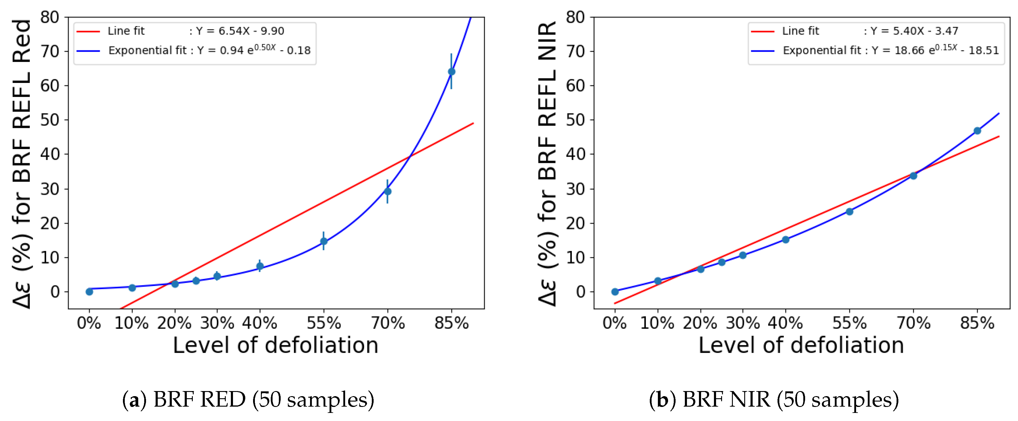
Figure 8.
Plot of defoliation vs relative variation for the different NDVI products. (a–d) are NDVI products calculated from TOA radiance, ELM-ideal, ELM-typical and BRF data respectively.
Figure 8.
Plot of defoliation vs relative variation for the different NDVI products. (a–d) are NDVI products calculated from TOA radiance, ELM-ideal, ELM-typical and BRF data respectively.

Figure 9.
NDVI calculated for the different data products as a function of defoliation. The NDVI for the TOA corrected products are lower than the NDVI for the surface reflectance products. This indicates that an accurate NDVI value can be estimated only when compensated for atmospheric attenuations.

Figure 10.
Difference in SZN angles between L8 and S2 over Harvard forest.


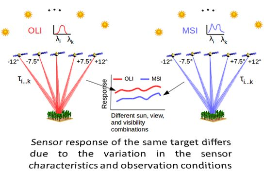
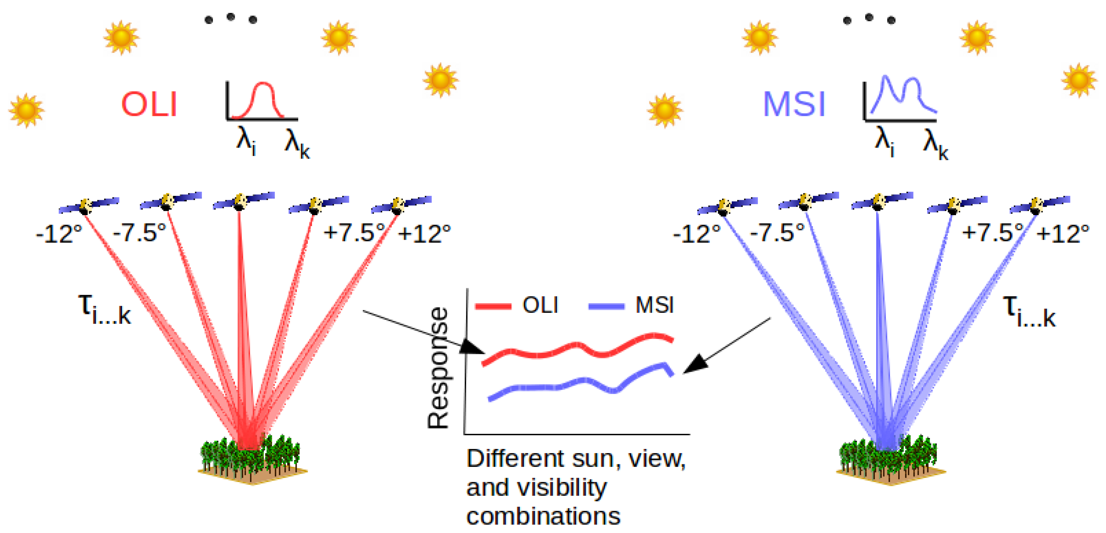
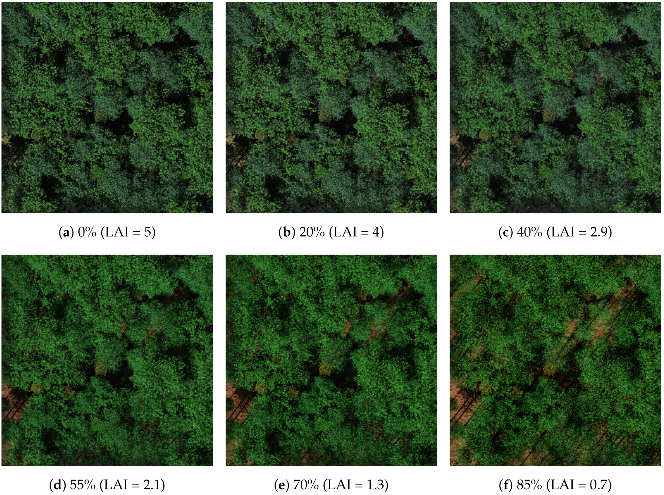
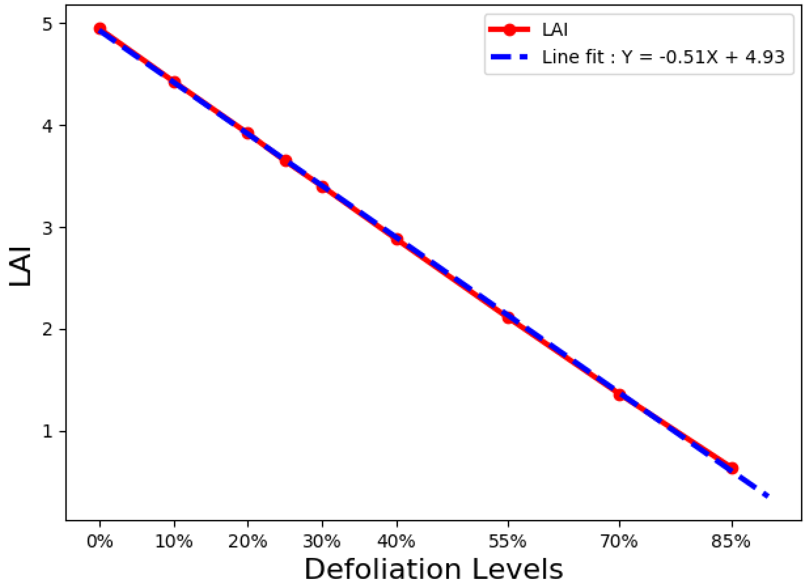
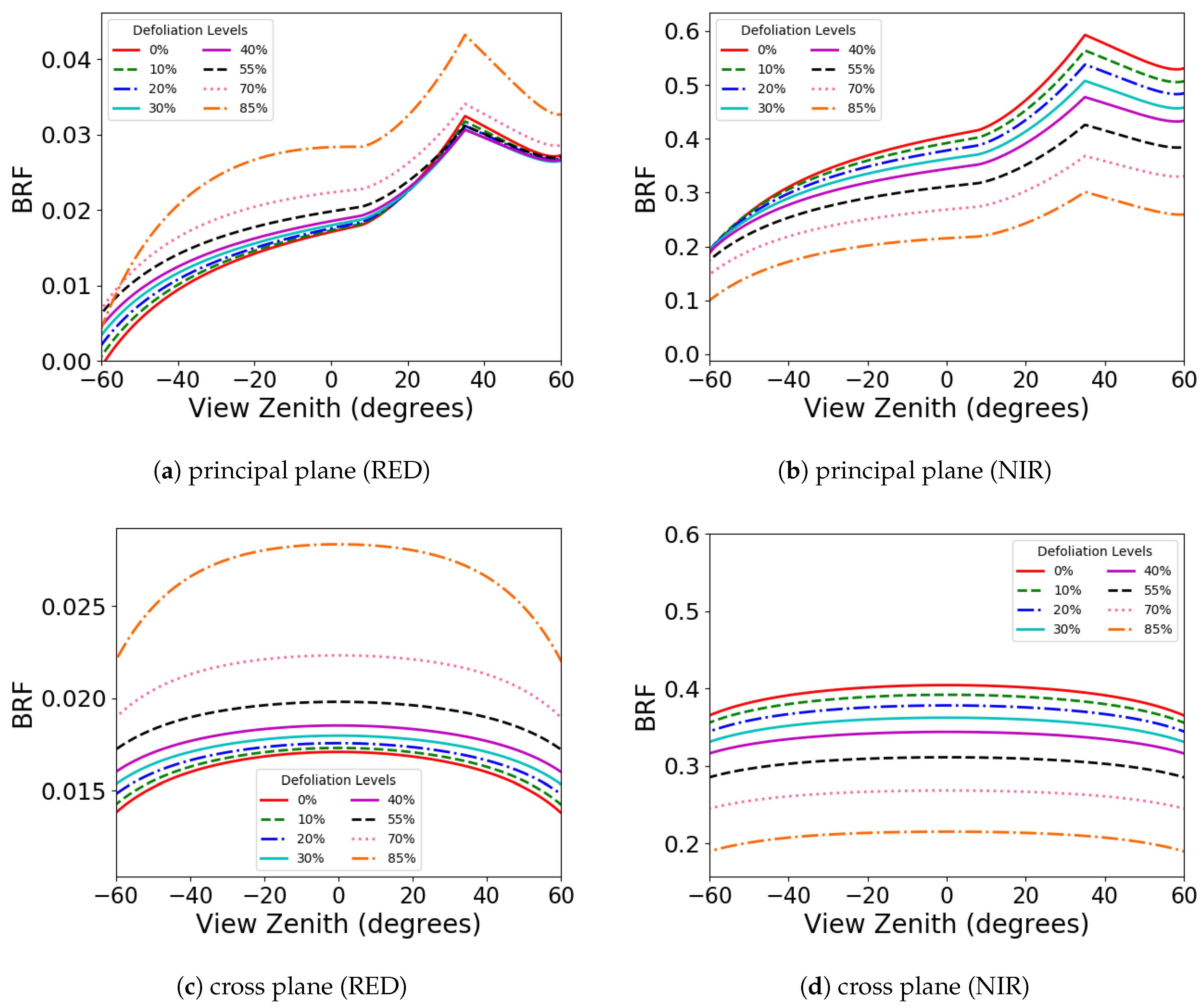
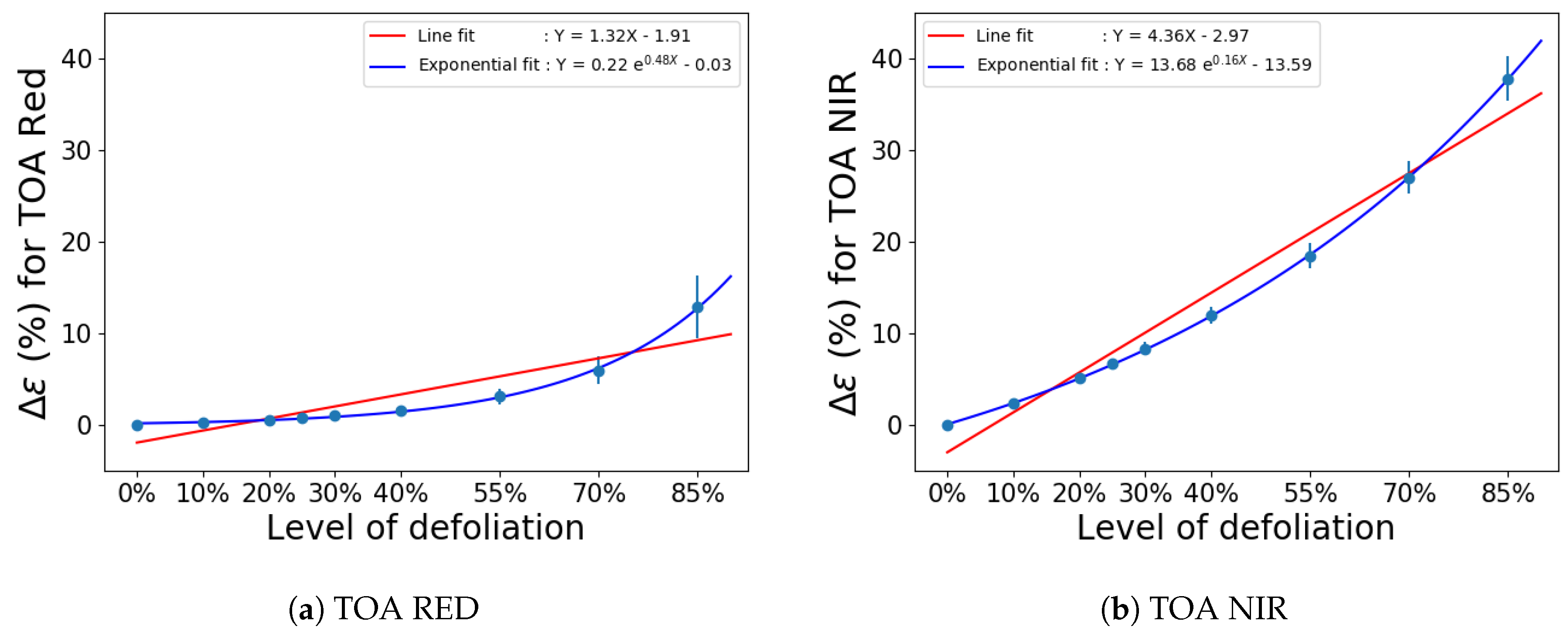
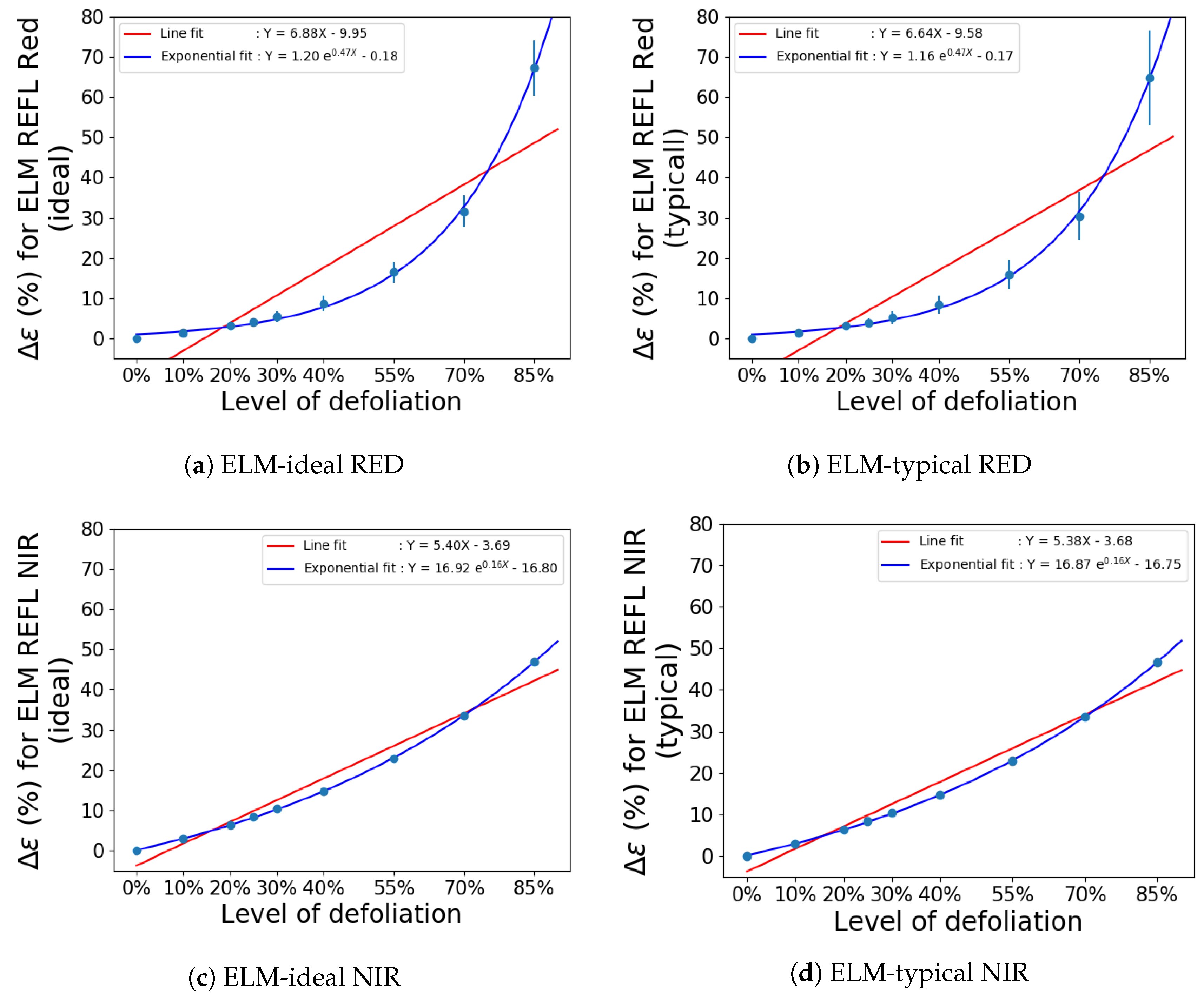
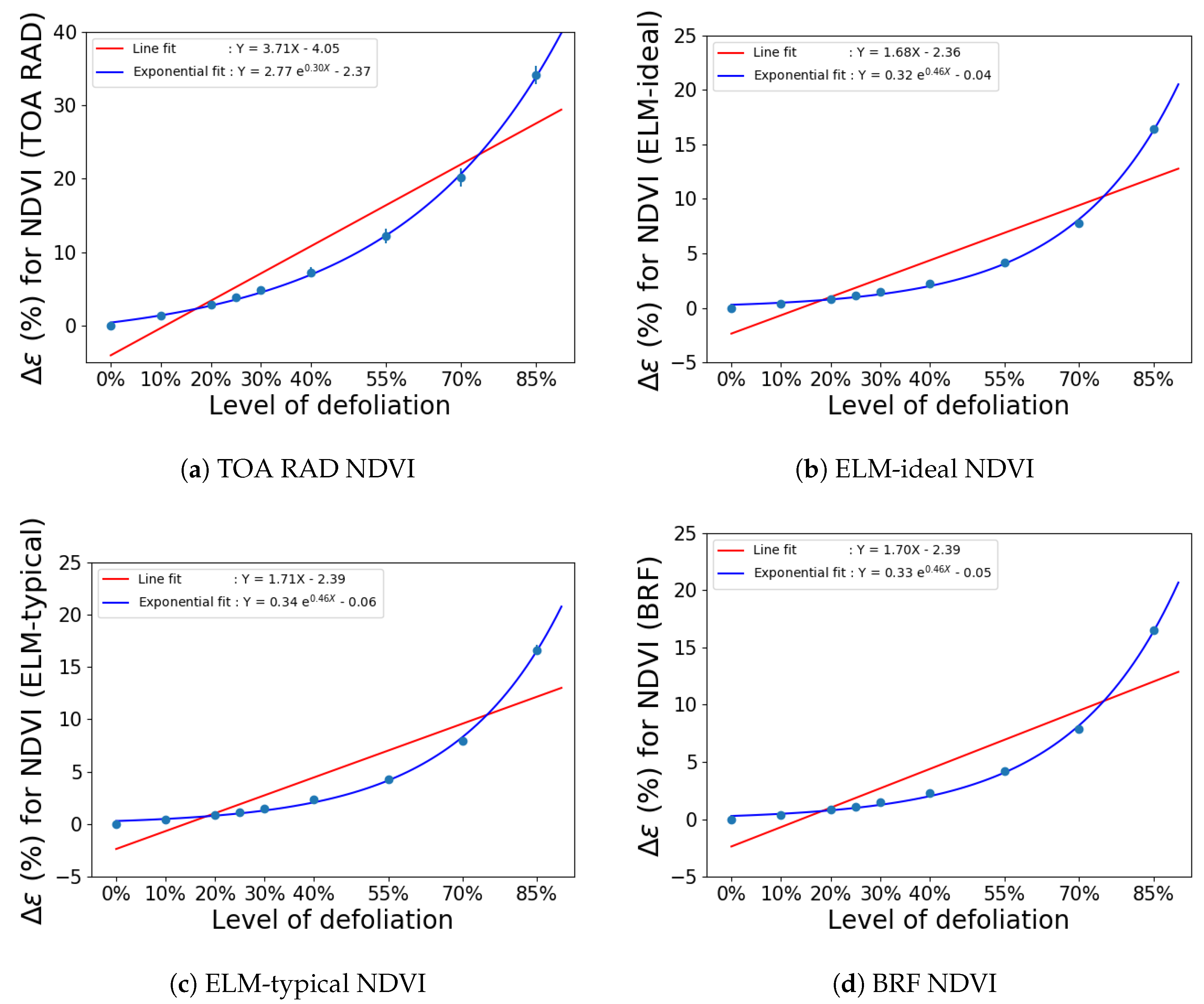
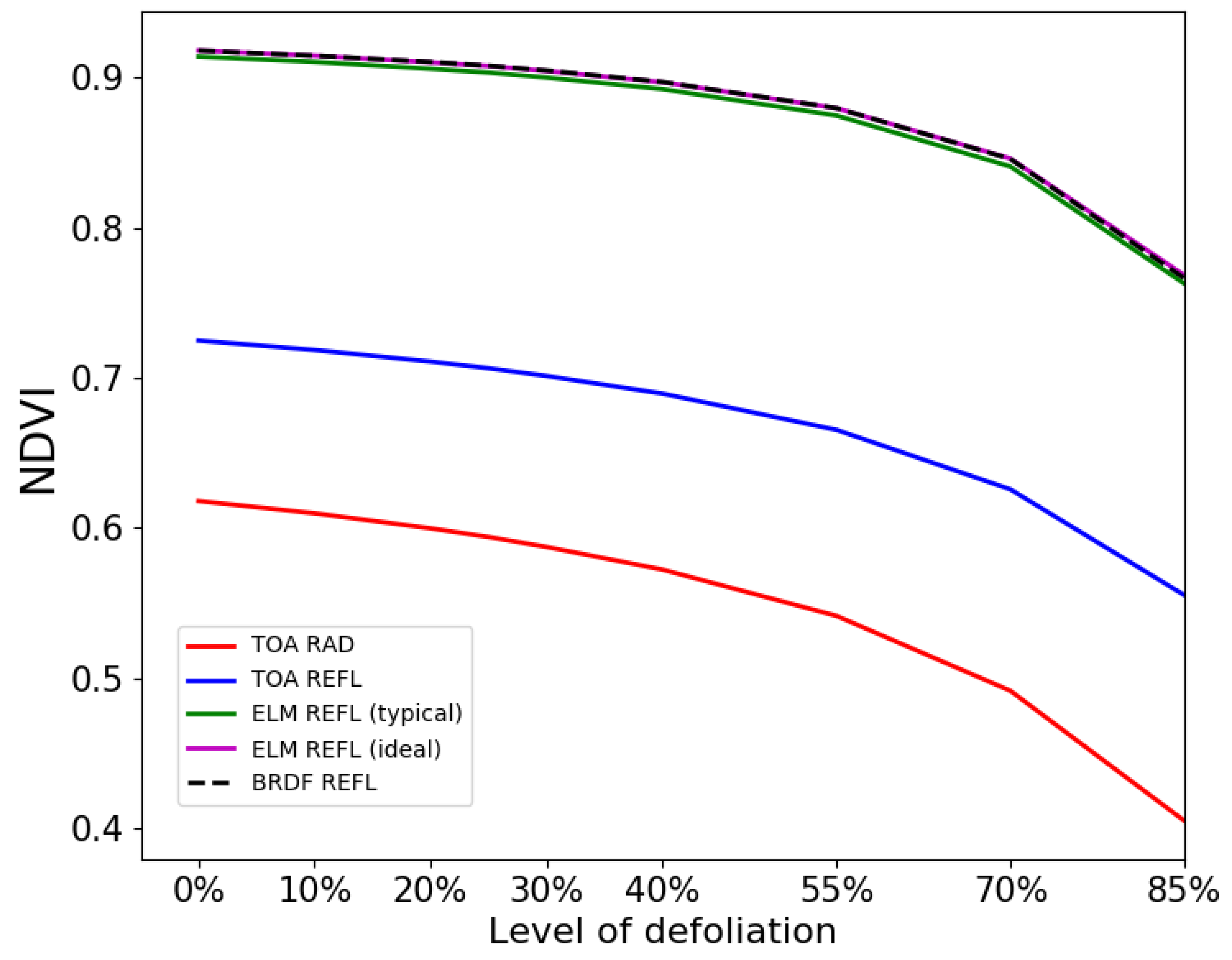
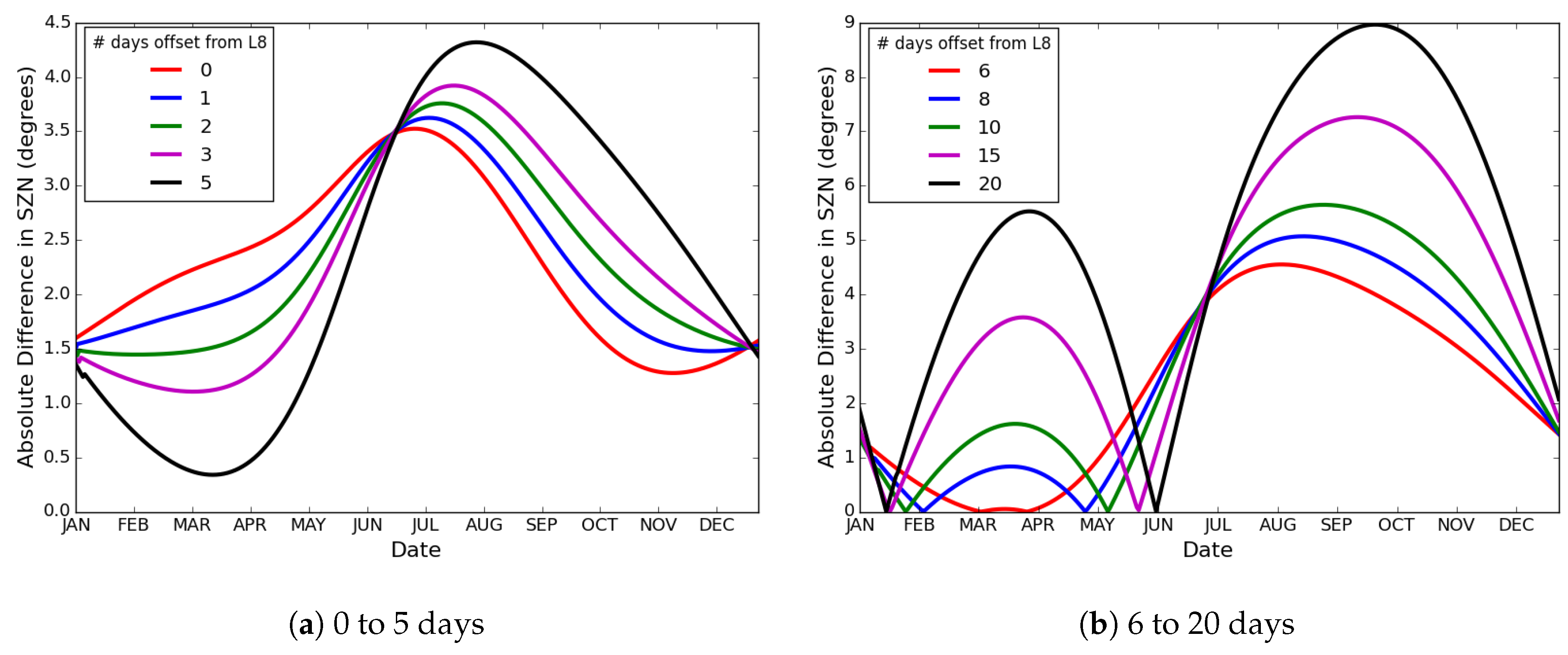
Table 1.
Sun angles, defoliation levels, X-Track angles, Visibility conditions, RSRs, and the spectral bands used in the sensitivity analysis.
Table 1.
Sun angles, defoliation levels, X-Track angles, Visibility conditions, RSRs, and the spectral bands used in the sensitivity analysis.
| Sun Angles | Defoliation | X-Track | Visibility | RSR | Spectral | |
|---|---|---|---|---|---|---|
| Zenith | Azimuth | Levels | Angles (deg) | (KM) | Bands | |
| 35 | 145 | 0% | −12 | 10 | OLI (L8) | RED |
| 30 | 137 | 10% | −7.5 | 15 | MSI (S2A) | NIR |
| 33 | 157 | 20% | 0 | 20 | ||
| 25 | 150 | 25% | 7.5 | 25 | ||
| 27 | 135 | 30% | 12 | |||
| 35 | 165 | 40% | ||||
| 20 | 150 | 55% | ||||
| 23 | 132 | 70% | ||||
| 40 | 150 | 85% | ||||
| 38 | 153 | |||||
Table 2.
Relative change as a function of different levels of defoliation for the products that are uncorrected (TOA RAD), corrected for planetary reflectance (TOA REFL), compensated for atmospheric attenuations (ELM-ideal, ELM-typical), and modeled surface reflectance (BRF) in the red spectral band. The mean values are used to fit an exponential curve to characterize the defoliation as a function of relative change.
| Level of Defoliation | Data Products in the Red Spectral Band | ||||
|---|---|---|---|---|---|
| TOA RAD μ (σ) | TOA REFL μ (σ) | ELM-Typical μ (σ) | ELM-Ideal μ (σ) | BRF μ (σ) | |
| 0% | 0 (0) | 0 (0) | 0 (0) | 0 (0) | 0 (0) |
| 10% | 0.25 (0.09) | 0.25 (0.09) | 1.32 (0.54) | 1.36 (0.48) | 1.05 (0.44) |
| 20% | 0.59 (0.19) | 0.59 (0.19) | 3.07 (1.05) | 3.17 (0.93) | 2.36 (0.86) |
| 25% | 0.75 (0.23) | 0.75 (0.23) | 3.85 (1.19) | 3.98 (1.04) | 3.25 (1.03) |
| 30% | 1.02 (0.31) | 1.02 (0.31) | 5.26 (1.54) | 5.45 (1.35) | 4.52 (1.36) |
| 40% | 1.64 (0.46) | 1.64 (0.46) | 8.40 (2.19) | 8.71 (1.84) | 7.55 (1.79) |
| 55% | 3.11 (0.83) | 3.11 (0.83) | 15.86 (3.57) | 16.44 (2.69) | 14.73 (2.61) |
| 70% | 6.00 (1.56) | 6.00 (1.56) | 30.40 (6.02) | 31.52 (3.99) | 29.16 (3.51) |
| 85% | 12.86 (3.42) | 12.86 (3.42) | 64.80 (11.84) | 67.21 (6.90) | 64.15 (5.21) |
Table 3.
Relative change as a function of different levels of defoliation for the products that are uncorrected (TOA RAD), corrected for planetary reflectance (TOA REFL), compensated for atmospheric attenuations (ELM-ideal, ELM-typical), and modeled surface reflectance (BRF) in the NIR spectral band. The mean values are used to fit an exponential curve to characterize the defoliation as a function of relative change.
| Level of Defoliation | Data Products in the Red Spectral Band | ||||
|---|---|---|---|---|---|
| TOA RAD μ (σ) | TOA REFL μ (σ) | ELM-Typical μ (σ) | ELM-Ideal μ (σ) | BRF μ (σ) | |
| 0% | 0 (0) | 0 (0) | 0 (0) | 0 (0) | 0 (0) |
| 10% | 2.39 (0.31) | 2.39 (0.31) | 2.95 (0.30) | 2.96 (0.30) | 3.18 (0.18) |
| 20% | 5.14 (0.48) | 5.14 (0.48) | 6.34 (0.34) | 6.36 (0.35) | 6.63 (0.29) |
| 25% | 6.70 (0.55) | 6.70 (0.55) | 8.27 (0.31) | 8.29 (0.32) | 8.54 (0.34) |
| 30% | 8.37 (0.70) | 8.37 (0.70) | 10.33 (0.45) | 10.36 (0.46) | 10.61 (0.42) |
| 40% | 11.97 (0.92) | 11.97 (0.92) | 14.78 (0.44) | 14.78 (0.44) | 15.18 (0.46) |
| 55% | 18.47 (1.36) | 18.47 (1.36) | 22.81 (0.55) | 22.81 (0.57) | 23.32 (0.54) |
| 70% | 27.07 (1.83) | 27.07 (1.83) | 33.44 (0.43) | 33.53 (0.45) | 33.81 (0.47) |
| 85% | 37.86 (2.45) | 37.86 (2.45) | 46.76 (0.28) | 46.90 (0.33) | 46.86 (0.37) |
Table 4.
Relative variation of the NDVI products for the different levels of defoliation. The values are used to relate the signal with the corresponding changes in the forest for factor sensitivity analysis.
Table 4.
Relative variation of the NDVI products for the different levels of defoliation. The values are used to relate the signal with the corresponding changes in the forest for factor sensitivity analysis.
| Level of Defoliation | NDVI Products | ||||
|---|---|---|---|---|---|
| TOA RAD μ (σ) | TOA REFL μ (σ) | ELM-Typical μ (σ) | ELM-Ideal μ (σ) | BRF μ (σ) | |
| 0% | 0 (0) | 0 (0) | 0 (0) | 0 (0) | 0 (0) |
| 10% | 1.30 (0.16) | 0.85 (0.10) | 0.38 (0.04) | 0.37 (0.03) | 0.37 (0.01) |
| 20% | 2.89 (0.30) | 1.89 (0.18) | 0.87 (0.08) | 0.84 (0.04) | 0.82 (0.03) |
| 25% | 3.80 (0.38) | 2.50 (0.22) | 1.14 (0.10) | 1.10 (0.04) | 1.100 (0.03) |
| 30% | 4.86 (0.47) | 3.19 (0.27) | 1.50 (0.12) | 1.45 (0.05) | 1.44 (0.04) |
| 40% | 7.26 (0.65) | 4.78 (0.37) | 2.33 (0.17) | 2.26 (0.07) | 2.27 (0.05) |
| 55% | 12.18 (0.94) | 8.06 (0.53) | 4.25 (0.26) | 4.14 (0.08) | 4.17 (0.07) |
| 70% | 20.16 (1.26) | 13.47 (0.69) | 7.97 (0.38) | 7.80 (0.10) | 7.85 (0.10) |
| 85% | 34.07 (1.27) | 23.14 (0.60) | 16.63 (0.50) | 16.39 (0.27) | 16.51 (0.21) |
Table 5.
Fit residuals between model and measured relative variation for 25% defoliation signal level. The red band shows consistently higher residuals than NIR.
Table 5.
Fit residuals between model and measured relative variation for 25% defoliation signal level. The red band shows consistently higher residuals than NIR.
| Data | RED | NIR | NDVI |
|---|---|---|---|
| Products | Relative Error | Relative Error | Relative Error |
| TOA Rad | 6.1% | 1.5% | 6.9% |
| TOA Refl | 6.1% | 1.5% | 7.4% |
| ELM-typical Refl | 6.3% | 1.5% | 10.9% |
| ELM-ideal Refl | 6.2% | 1.5% | 10.9% |
| BRF Refl | 5.3% | 0.9% | 10.6% |
Table 6.
Effect of RSR for NDVI products before and after SBAF compensation. The effects are shown in NED units, i.e, the percentage implies that the effect due to RSR is equivalent to an actual level of defoliation.
Table 6.
Effect of RSR for NDVI products before and after SBAF compensation. The effects are shown in NED units, i.e, the percentage implies that the effect due to RSR is equivalent to an actual level of defoliation.
| Data | Uncompensated | SBAF (TOA REFL) | SBAF (BRF) |
|---|---|---|---|
| Products | Mean (STD) | Mean (STD) | Mean (STD) |
| NDVI TOA Rad | 19% (2.2%) | 2% (1.3%) | 7% (3.4%) |
| NDVI TOA Refl | 19% (1.9%) | 2% (1.3%) | 7% (3.2%) |
| NDVI ELM-typical Refl | 15% (1.5%) | 3% (0.6%) | 1% (0.9%) |
| NDVI ELM-ideal Refl | 15% (0.8%) | 3% (0.5%) | 1% (0.5%) |
Table 7.
Effect of across-track angle for NDVI products before and after SBAF compensation. The effects are shown in NED units.
Table 7.
Effect of across-track angle for NDVI products before and after SBAF compensation. The effects are shown in NED units.
| Data | Uncompensated | SBAF (TOA REFL) | SBAF (BRF) |
|---|---|---|---|
| Products | Mean (STD) | Mean (STD) | Mean (STD) |
| NDVI TOA Rad | 17% (8.8%) | 8% (5.7%) | 11% (8.2%) |
| NDVI TOA Refl | 17% (8.6%) | 8% (5.7%) | 10% (8.1%) |
| NDVI ELM-typical Refl | 28% (21.5%) | 28% (21.3%) | 28% (21.9%) |
| NDVI ELM-ideal Refl | 16% (5.0%) | 5% (3.8%) | 4% (2.7%) |
| NDVI BRF Refl | 5% (2.8%) | 5% (2.8%) | 5% (2.8%) |
Table 8.
Effect of two extreme view angles (±12°) for NDVI products before and after SBAF compensation. The effects are shown in NED units. Since the effect estimate calculation is independent of the sensor, the SBAF compensation does not show any improvements.
Table 8.
Effect of two extreme view angles (±12°) for NDVI products before and after SBAF compensation. The effects are shown in NED units. Since the effect estimate calculation is independent of the sensor, the SBAF compensation does not show any improvements.
| Data | Uncompensated | SBAF (TOA REFL) | SBAF (BRF) |
|---|---|---|---|
| Products | Mean (STD) | Mean (STD) | Mean (STD) |
| NDVI TOA Rad | 14% (4.6%) | 14% (4.7%) | 14% (4.8%) |
| NDVI TOA Refl | 14% (4.5%) | 14% (4.7%) | 14% (4.7%) |
| NDVI ELM-typical Refl | 40% (21.7%) | 40% (22.1%) | 40% (22.2%) |
| NDVI ELM-ideal Refl | 9% (2.6%) | 9% (3.8%) | 9% (2.7%) |
| NDVI BRF Refl | 10% (3.2%) | 10% (3.2%) | 10% (3.2%) |
Table 9.
Effect of visibility for NDVI products before and after the SBAF compensation. The effects are shown in NED units.
Table 9.
Effect of visibility for NDVI products before and after the SBAF compensation. The effects are shown in NED units.
| Data | Uncompensated | SBAF (TOA REFL) | SBAF (BRF) |
|---|---|---|---|
| Products | Mean (STD) | Mean (STD) | Mean (STD) |
| NDVI TOA Rad | 40% (39%) | 40% (40%) | 40% (39%) |
| NDVI TOA Refl | 40% (38%) | 40% (39%) | 40% (38%) |
| NDVI ELM-typical Refl | 16% (10%) | 8% (9%) | 7% (9.7%) |
| NDVI ELM-ideal Refl | 15% (1.4%) | 4% (1.3%) | 1% (0.9%) |
Table 10.
Effect for 5° difference in SZN angles for NDVI products before and after SBAF compensation. The effects are shown in NED units.
Table 10.
Effect for 5° difference in SZN angles for NDVI products before and after SBAF compensation. The effects are shown in NED units.
| Data | Uncompensated | SBAF (TOA REFL) | SBAF (BRF) |
|---|---|---|---|
| Products | Mean (STD) | Mean (STD) | Mean (STD) |
| NDVI TOA Rad | 10% (5%) | 10% (5%) | 10% (5%) |
| NDVI TOA Refl | 10% (5%) | 10% (5%) | 10% (5%) |
| NDVI ELM-typical Refl | 8% (7%) | 8% (7%) | 8% (7%) |
| NDVI ELM-ideal Refl | 4% (1.4%) | 4% (1.4%) | 4% (1.4%) |
| NDVI BRF | 4% (1.6%) | 4% (1.6%) | 4% (1.6%) |
© 2018 by the authors. Licensee MDPI, Basel, Switzerland. This article is an open access article distributed under the terms and conditions of the Creative Commons Attribution (CC BY) license (http://creativecommons.org/licenses/by/4.0/).
Share and Cite
MDPI and ACS Style
Rengarajan, R.; Schott, J.R. Evaluation of Sensor and Environmental Factors Impacting the Use of Multiple Sensor Data for Time-Series Applications. Remote Sens. 2018, 10, 1678. https://doi.org/10.3390/rs10111678
AMA Style
Rengarajan R, Schott JR. Evaluation of Sensor and Environmental Factors Impacting the Use of Multiple Sensor Data for Time-Series Applications. Remote Sensing. 2018; 10(11):1678. https://doi.org/10.3390/rs10111678
Chicago/Turabian StyleRengarajan, Rajagopalan, and John R. Schott. 2018. "Evaluation of Sensor and Environmental Factors Impacting the Use of Multiple Sensor Data for Time-Series Applications" Remote Sensing 10, no. 11: 1678. https://doi.org/10.3390/rs10111678
Note that from the first issue of 2016, this journal uses article numbers instead of page numbers. See further details here.