Estimating Calibration Variability in Evapotranspiration Derived from a Satellite-Based Energy Balance Model

Department of Civil and Environmental Engineering, University of Utah, 110 S. Central Campus Drive, Salt Lake City, UT 84112, USA
*
Author to whom correspondence should be addressed.
Remote Sens. 2018, 10(11), 1695; https://doi.org/10.3390/rs10111695
Submission received: 21 September 2018
/
Revised: 19 October 2018
/
Accepted: 24 October 2018
/
Published: 26 October 2018
(This article belongs to the Special Issue Remote Sensing of Evapotranspiration (ET))
Abstract
:Computing evapotranspiration (ET) with satellite-based energy balance models such as METRIC (Mapping EvapoTranspiration at high Resolution with Internalized Calibration) requires internal calibration of sensible heat flux using anchor pixels (“hot” and “cold” pixels). Despite the development of automated anchor pixel selection methods that classify a pool of candidate pixels using the amount of vegetation (normalized difference vegetation index, NDVI) and surface temperature (Ts), final pixel selection still relies heavily on operator experience. Yet, differences in final ET estimates resulting from subjectivity in selecting the final “hot” and “cold” pixel pair (from within the candidate pixel pool) have not yet been investigated. This is likely because surface properties of these candidate pixels, as quantified by NDVI and surface temperature, are generally assumed to have low variability that can be attributed to random noise. In this study, we test the assumption of low variability by first applying an automated calibration pixel selection process to 42 nearly cloud-free Landsat images of the San Joaquin area in California taken between 2013 and 2015. We then compute Ts (vertical near-surface temperature differences) vs. Ts relationships at all pixels that could potentially be used for model calibration in order to explore ET variance between the results from multiple calibration schemes where NDVI and Ts variability is intrinsically negligible. Our results show significant variability in ET (ranging from 5% to 20%) and a high—and statistically consistent—variability in dT values, indicating that there are additional surface properties affecting the calibration process not captured when using only NDVI and Ts. Our findings further highlight the potential for calibration improvements by showing that the dT vs. Ts calibration relationship between the cold anchor pixel (with lowest dT) and the hot anchor pixel (with highest dT) consistently provides the best daily ET estimates. This approach of quantifying ET variability based on candidate pixel selection and the accompanying results illustrate an approach to quantify the biases inadvertently introduced by user subjectivity and can be used to inform improvements on model usability and performance.
1. Introduction
Evapotranspiration (ET) is an essential part of any hydrologic investigation as it represents the flux of water between soils, plants, and biosphere [1]. Since 75% of the world’s freshwater withdrawals support agriculture [2], estimating ET as consumptive use accurately over a watershed is crucial for efficient water resources planning [3]. ET can be assessed at different scales of observation with multiple approaches and methods [4] such as the field-scale water balance approach using weighing lysimeter [5], the field-scale energy balance approach using the Eddy Covariance (EC) technique [6] and scintillometers [7], and the leaf- or plant-scale energy balance approach using Sap-flow techniques [8]. These methods vary in size of effective area measured, cost, complexity, and accuracy. However, the footprint of field ET measured by these methods is smaller than the watershed area, usually by orders of magnitude, which often creates significant discrepancies in ET estimates at spatial scales larger than plot or field scales [9]. Most commonly, ET over an agricultural region is measured by multiplying a weather-based estimate of reference ET by crop coefficients (which can vary with crop type and crop growth stage) [10]. This method of estimating ET is popular since it can be applied with ease. However, since crop growth and vegetative stage can vary significantly even for the same crop in a watershed due to spatial variability in soil, fertilization and irrigation practice, slope, basin orientation, temperature, and numerous other factors [11], this method of estimating watershed ET requires multiple assumptions and increases uncertainty in the results. Uncertainties can propagate directly or indirectly (i.e., through additional hydrologic models) into decision-making processes of water right managers, water resource planners, ecologists, and researchers, potentially causing issues such as inaccurate allocation of water rights, higher redundancies or deficiencies in water infrastructure, and inaccurate estimates of ecological flows [12,13,14].
To overcome these problems, remotely sensed data have been used in conjunction with surface energy balance models to estimate ET [15]. Of the many surface-energy-balance-based remote sensing models available, this work uses the Mapping EvapoTranspiration at high Resolution using Internalized Calibration (METRIC) model since it was specifically designed for agricultural areas and parameterized according to the factors most relevant to the characteristics of our study area. It was also chosen since it uses freely available Landsat satellite imageries that are taken every 16 days, thereby capturing the vegetation growth stages within a watershed.
ET is estimated in METRIC by taking the energy consumed by the ET process as a residual of the surface energy balance equation [16]. This energy is called latent heat flux (LE) [W/m2] and is represented by
where the net radiation, Rn, is the balance of all incoming and outgoing short-wave and long-wave radiation [W/m2], G is the soil heat flux [W/m2], and H is the sensible heat flux [W/m2].
Although METRIC has been proven to be a powerful tool in estimating evapotranspiration for larger areas, the accuracy and final results depend on user selection of parameters, submodels for calculation of components in energy balance, and calibration pixels [16]. Acknowledging this, Allen et al. [17] states that anchor pixel selection used in the calibration process (called CIMEC—Calibration using Inverse Modeling at Extreme Conditions) can correct for lingering biases in parameter selection associated with estimation of albedo, atmospheric correction, land surface temperature, emissivity, soil heat flux, and net radiation. This makes calibration of METRIC one of the most important steps in obtaining accurate ET estimates. The calibration process in METRIC requires identifying a “hot” and “cold” anchor pixel pair based on extreme conditions within a given image. In such an image, a well-irrigated pixel with maximum possible evapotranspiration is considered to be “cold”, and a dry field with almost no evapotranspiration is “hot”. Selecting these pixels, however, requires careful consideration of properties other than surface temperature (Ts), including normalized difference vegetation index (NDVI), surface albedo, and land use type. In the past, calibration pixel selection was completely dependent on expert judgement, but researchers have recently begun creating processes to automatically identify a subset of pixels from which the final selection is made [18,19]. Although METRIC has been used by water resource managers for a variety of applications such as water rights management, water allocation, and estimation of water yield, the need for expert judgement in the calibration process makes METRIC a complicated tool for operational use. A calibration process that facilitates a completely automatic application of METRIC would significantly expand its use as an operational model rather than primarily as a research tool.
One of these automatic pixel selection algorithms, a statistics-based procedure by Allen et al. [19], simplifies the techniques traditionally requiring extensive knowledge of remote sensing processes and vegetation indices. Although their procedure significantly reduces the number of potential anchor pixels, the final pair must still be selected using expert judgement. Furthermore, while the METRIC model itself has been validated (e.g., Bhattarai et al. [20] using a process similar to the procedure explained in Allen et al. [19]), no attempt has been made to evaluate ET results from the model calibrated using pixels from automated calibration. Rather, previous evaluations of the automated calibration pixel selection processes [18,19] have only compared the temperature of the anchor pixels selected by an expert to the temperature of the pixels selected by the algorithm.
A study by Morton et al. [21] has, to a certain extent, evaluated calibration uncertainty in METRIC ET results by applying a calibration process similar to that used by Allen et al. [19], and concluded that automatic calibration processes can produce ET estimates very similar to time-intensive manual efforts. Morton’s study used a distribution of reference ET fraction (ETrF) computed for the specific study area using METRIC results from five trained users. Although Morton’s method would help in automating the calibration of METRIC, two major limitations prevent the uptake of the method by a general METRIC user: (1) it involves a computationally intensive procedure (Monte Carlo simulation), and (2) it requires a generic cumulative distribution function (CDF) of ETrF for the study regions (which is usually lacking).
In this paper, with an objective of estimating the calibration variability in METRIC ET, we examine the properties of anchor pixels selected by automatic procedures and identify additional properties other than NDVI and Ts that affect calibration processes. To do so, five sets of calibration pixel pairs, encompassing all possible combinations, were prepared using all available calibration pixel sets. These calibration sets were then used to find the variation in ET. Previous studies suggest that, based on the nature of the automatic calibration pixel selection process, only small and random variations of final ET should occur when using this approach. However, our results indicated significant spatial differences in ET across the study area. Furthermore, one of the five sets we investigated provided consistently better results across multiple years, showing that NDVI and surface temperature alone do not capture all relevant surface properties required for the calibration pixel selection process. These results will be useful in operational aspects of METRIC calibration, allowing the user to be aware of the variability in ET results caused by calibration pixel selection.
2. Materials and Methods
2.1. Study Area
This study focused on an agricultural area in San Joaquin—Sacramento River Delta area (Figure 1 and Table 1). A U.S. AmeriFlux site with an EC flux tower in the area was used to compare and quantify the variability in ET due to the calibration pixel selection process in METRIC. The farm plot (Twitchell Alfalfa) has been used to farm alfalfa, with crop rotation occurring every 5–6 years. The alfalfa at the site is harvested by mowing and bailing several times per year and is irrigated periodically by flooding ditches around the field [22]. Based on the recommended procedure developed by Allen et al. [19], we selected calibration pixels from a study area within a 30 km radius around the available weather station (Figure 1).
2.1.1. Measured ET Data
An Eddy Covariance (EC) system with GILL WM 1590 sonic anemometers and a LICOR LI-7500A CO2/H2O gas analyzer was used at the flux site. Daily flux data from this site was postprocessed and provided as 30 min average datasets [23]. The EC instruments were mounted at a height of 2.8 m above the ground.
2.1.2. Landsat Images
We performed our analysis with Landsat images since this allows ET to be mapped at field scales. Additionally, ET measured using an EC tower has a fetch of about 100 times [24] the station height, so METRIC results using Landsat will give an accurate representation of the area around the station.
We used all available nearly cloud-free Landsat 7 (With Enhanced Thematic Mapper Plus or ETM+ sensor) and Landsat 8 (with Operational Land Imager or OLI sensor) images covering the station within the ET measurement period (Table 2). Even though the satellite images are captured using different sensors, Kilic et al. [25] did not find significant differences in NDVI and ETrF computed from these imageries. Therefore, we did not treat these images differently in our study. The cloud mask created using the CFMask algorithm [26], provided within the Landsat Collection 1 Level-1 Quality Assessment (QA) band, was used to determine cloudy pixels. Only images with less than 20% cloud coverage (by area) were used. To remove cloudy images not identified by CFMask and QA bands, the weather station and validation site location in these images were visually inspected using a contrast enhancement function provided by Google Earth Engine (GEE) [27] (see Section 2.3). This function uses a Styled Layer Descriptor (SLD) to render red, green, and blue bands that produce images with equal brightness levels. Rather than download Landsat imageries, we used GEE to access and analyze Landsat data from the public catalog GEE provides.
2.1.3. Weather Data
Freely available hourly meteorological data from the California Irrigation Management Information System (CIMIS) (last accessed 17/11/2017) was used for this study. Specifically, we used CIMIS Station Number 140 (Twitchell Island) in Sacramento, CA since this is the only site that has data for the complete study period.
2.1.4. Land Cover Data
Land cover data available in the GEE catalog from the USGS National Land Cover Database 2011 were used to identify the agricultural land use pixels and pasture land use pixels required for this study.
2.2. METRIC Model
METRIC is a satellite-based image processing model that computes ET as the residual of energy balance as given in Equation (1) above. METRIC first computes available energy as (Rn − G), which is then divided into LE and H. In our work, the components of energy balance needed to compute Rn were estimated using the formulations provided in Allen et al. [16] and Allen et al. [17]. In these studies, the formulations have been provided in detail for Landsat 5 and 7. However, since we also included Landsat 8 for our studies, there were a few components which we had to formulate using related newer studies.
These components include surface albedo, α, which was computed for Landsat 8 using weighing coefficients based on Ke et al. [28]. They used the Simple Model of Atmospheric Radiative Transfer of Sunshine (SMARTS) radiative transfer model to determine the weighing coefficients for Landsat 8 OLI sensors. This is similar to the procedure used in Tasumi et al. [29] to compute surface albedo for Landsat 5 TM and Landsat 7 ETM+ sensors. Due to the consistency between the two methods of calculating albedo using weights for each band of similar wavelengths across different satellite sensors, significant biases in the reflected solar radiation were not introduced into the model [30].
Surface temperature was computed based on the single channel method outlined in Sobrino et al. [31] for Landsat 5, Jimenez-Munoz et al. [32] for Landsat 7, and Yu et al. [33] for Landsat 8. Of the two bands in Landsat 7 that can be used to compute radiometric surface temperature, we used the high gain band (VCID_2) since our analysis required better estimates of temperature for vegetated areas. Similarly, from the two Thermal Infrared Sensor (TIRS) bands of Landsat 8, band 10 was used since band 11 is known to have larger calibration uncertainty [34]. In addition to thermal bands, this method requires land surface emissivity (ε) and water vapor content (w) to compute surface temperature. Water vapor content (w) was used from the weather station data and emissivity (ε) was computed using the NDVI threshold method.
The remaining components of energy balance for the model were computed using Allen et al. [17]. Of the multiple soil heat flux relationships available, our study used the following relation which uses net radiation (Rn) to compute soil heat flux [16,35,36]:
Sensible heat flux (H), which is one of the key components of METRIC, is estimated using a one-dimensional bulk aerodynamic temperature-gradient-based method as
where ρ is the air density (kg/m3), cp is the air specific heat at constant pressure (J/kg K), rah1,2 is the aerodynamic resistance (s/m) between two heights Z1 and Z2 above the zero-plane displacement height of vegetation (zom) where endpoints of dT are defined, and dT is the vertical near-surface temperature difference (K). The near-surface heights Z1 and Z2 are assumed to be 0.1 m and 2 m above the zero-plane displacement height (zom).
The value of rah1,2 is calculated using wind speed extrapolated from some blending height above the ground surface (typically 200 m) and using an iterative stability correction scheme based on Monin–Obhukhov functions [37,38]. An iterative solution is needed because this aerodynamic resistance (rah1,2) is influenced by the buoyancy caused by surface heating which is driven in turn by the sensible heat Flux (H), and both rah1,2 and H are unknown at a given pixel.
The parameter dT, which is the difference in temperature at two near-surface heights (usually Tz1 = 0.1 + zom and Tz2 = 2.0 + zom), is difficult to compute directly because the temperatures at these two levels estimated from satellite sensors will have uncertainties greater than their differences [16]. To overcome this issue, METRIC uses an approach developed by Bastiaanssen [35] that approximates dT as a linear function of Ts given by
where a and b are regression coefficients. These coefficients are determined using a procedure that first selects two extreme condition pixels in the image, one which represents maximum LE (cold pixel) and the other which represents minimum or zero LE (hot pixel), then implements Equations (1) and (3) on these pixels. Bastiaanssen [39] assumed that, at a cold pixel, all available energy is used up for latent heating, so H ≈ 0. At a hot pixel, conversely, all available energy is used up for sensible heat flux, so LE ≈ 0. For the METRIC application, it is assumed that the latent heat flux corresponds to the ET value that is 5% more than the ASCE (American Society of Civil Engineers) standardized alfalfa-based reference ET at a selected cold pixel. Similarly, it is assumed that, at a selected hot pixel, the latent heat flux corresponds to the ET value that is bare soil ET due to prior precipitation events calculated using the FAO-56 soil water evapotranspiration model [10,17]. An iterative solution approach is then applied at these two “anchor” pixel locations to determine dT and, subsequently, the relationship between dT and Ts. Readers are referred to Allen et al. [17] for more details on the iterative process.
2.3. Google Earth Engine for METRIC
We used Google Earth Engine (GEE) [27] and the associated Python API to develop and implement METRIC in an entirely web-based environment that does not require download of any raster data (Landsat, Digital Elevation Model (DEM), and land use) or use of a personal computational engine. GEE is a cloud-based geospatial processing platform developed by Google Inc. and combines large (petabyte scale) storage capabilities, which contain archived remotely sensed imageries, with a powerful computational infrastructure optimized for parallel processing of large geospatial datasets. It also supports charting, dynamic mapping, and table/image export features, making it easier to visualize intermediate results without needing to download anything onto a personal computer. Additionally, most of the GEE’s algorithms use per-pixel algebraic functions, making it ideal to apply irrespective of the region or scale (provided that the data are available for the region).
2.4. Selection of Calibration Pixels
An overview of the modeling process with selection of calibration pixels for this study is presented in Figure 2. We used the process outlined in Allen et al. [19] and Bhattarai et al. [18] to select the sets of candidate calibration pixels. The selection of candidate calibration pixels using the method outlined by Bhattarai et al. [18] provided a smaller subset from within those pixels selected using Allen et al. [19], because we iteratively increased the window size in small increments for NDVI and Ts as suggested by the authors. This resulted in a final window size which was much smaller for the former method than the latter one. Although the selection method outlined by Bhattarai et al. [18] provides a smaller set of calibration pixels and has been shown to perform with comparable accuracy in the final ET results when compared to the method used by Allen et al. [19], we used the latter method since our goal was to understand the variability in dT between candidate pixels due to small variations in Ts and NDVI. Additionally, the calibration pixel selection process developed by METRIC developers (i.e., Allen et al. [16]) is considered a standard method and has been recently used in Earth Engine Evapotranspiration Flux (EEFlux) [40].
The study area for this work was selected following Allen et al. [19] who suggest an area with a radius of 20–30 km around the weather station to be used for calibration of the model for the given image. Since the elevation around our weather station does not change drastically, we assume that the elevation adjusted temperature, determined using a customized lapse rate (TsDEM), and wind speed across the terrain [41], which is used for calibration, do not change drastically. Due to the minimal elevation differences, we used an area with the maximum possible radius of 30 km suggested by Allen et al. [19]. The corrections for temperature with elevation (TsDEM) and wind speed were, however, performed for this study using Allen et al. [17] and Allen et al. [41]. If there are significant changes in elevation which could affect TsDEM or wind speed, the area used for calibration needs to be divided into regions with similar elevation and climate, and terrain corrections applied.
Within the 30 km radius area, we used pixels with land use (LU) classified as Pasture/Hay, Cultivated Crops, and Grassland (LU codes 81, 82, and 71, respectively). The selected pixels were filtered as recommended by Allen et. al [19] to eliminate effects of clouds, field edges for thermal pixels, and Ts vs. NDVI relationships. For homogeneity in the thermal pixels, we filtered the image using a 7 × 7 pixel cluster and rejected any pixels having a standard deviation greater than 1.5 K, as recommended by Bhattarai et al. [18]. Similarly, to avoid too much variation in NDVI within calibration polygons, we rejected pixels with coefficients of variation (Standard Deviation/Mean) greater than 0.15 (per [19]). Some images had clouds not identified by the F-mask algorithm in QA bands; these were manually delineated before calibration.
2.4.1. Hot and Cold Pixel Set Identification
Allen et al. [19] states that a cold pixel candidate can been found to lie in the coolest, most vegetated 1% of areas within the image (the coldest 20% of the 5% highest vegetated pixels). Similarly, a hot pixel candidate can been found to lie in the hottest, least vegetated 2% of the image (the warmest 20% of the 10% lowest pixels). So, we followed Allen et al. [19], which has been used successfully for finding calibration pixels, so that the method of the calibration pixel selection process would be consistent with other similar applications of METRIC [21,42]. Additionally, since the model is used for estimating consumptive use in agricultural watersheds, we assume that there will be ample agricultural pixels during the growing season other than dry bare pixels, so a larger subset of hot pixels was selected than of cold pixels for our analysis.
To identify cold pixels, the pixels with top 5% NDVI were first isolated. From these pixels, those with the lowest 20% of Ts were further selected. This provided a sample of 1% of the coldest pixels having the highest NDVI and lowest temperature. From this 1% set, the cold pixels were then chosen to be within ±0.2 K of the average temperature and within ± 0.02 of the albedo threshold calculated using the equation provided in Allen et al. [19], which was parameterized for Southern Idaho, as follows:
where α is the albedo threshold and β is the sun angle above the horizon.
Computing the albedo threshold using Equation (5) resulted in most of the cold pixel albedo values falling between 0.18 and 0.25, which is within the suggested range of albedo for a representative reference alfalfa (0.23). Also, since the study was performed during growing seasons with higher β values, we did not change the parameters of Equation (5).
Like NDVI, the Soil Adjusted Vegetation Index (SAVI) [43] is another common vegetation index that provides useful information on vegetation growth. However, since NDVI has a more linear means of specifying the reference ET fraction compared to SAVI [19], we only used NDVI during the calibration pixel selection process. To verify this assumption, SAVI values were calculated for both cold and hot candidate pixels. The distributions of these values are shown in the Supplementary Materials section of this paper (Figure S1). The horizontal line where SAVI equals 0.69 indicates when Leaf Area Index (LAI) becomes “saturated” (LAI ≥ 6.0). Above this, the leaf area does not vary significantly. In Figure S1, we note that SAVI values can exceed the full LAI conditions. However, ETrF and crop coefficients (Kc) tend to reach maximum values near full-cover conditions, same as the NDVI [44]. Thus, in this case, NDVI was the correct choice for the cold pixel selection process.
To identify hot pixels, the lowest 10% NDVI pixels isolated from the candidate pixels were first selected. From these, the hottest 20% of Ts pixels were then selected. This provided a sample of 2% of the hottest pixels with lowest NDVI from the candidate pixels. Hot pixels within ±0.2 K of the average temperature were then chosen from this 2% set. The reference ETrF for this pixel was then computed using ETrFbare from the water balance model provided in FAO-56 [10]. Hot pixels were selected from regions of homogenous agricultural land use having bare soil conditions and, therefore, low values of NDVI. Bare soil pixels in some cases have vegetation residue but still have low NDVI values [45]. These pixels with organic cover need to be removed from the calibration set because the insulation provided by this cover can reduce soil heat flux (G) which may not be accurately captured by the relationship developed to estimate G in our study. Some of these low NDVI pixels with vegetative cover have higher albedo values than dry bare soil [46]. So, to remove pixels with organic cover within our hot candidate calibration pixel set, we removed hot pixels which had albedo values higher than 0.30~0.35 [19]. The sets of hot and cold pixels were then used to determine the dT vs. Ts relation for calibration of the model.
2.4.2. Determination of the dT vs. Ts Relationship from Selected Candidate Pixels
Values of dT computed from each hot and cold pixel selected from the step above were used to plot dT vs. Ts and identify the variations possible in calibration relations. Five sets of calibration pixel pairs were then selected from these possible calibration relations (Figure 3). These were selected so that the intercept and slope of the calibration line (“a” and “b” from Equation (4)) would encompass every possible relation within these available sets of calibration pixels.
The first set of calibration pixel pairs consists of a cold pixel with the lowest dT value and a hot pixel with the lowest dT value (Figure 3). This pair of pixels is referred to as the “Min Min” set hereafter (minimum cold pixel dT and minimum hot pixel dT). Similarly, the second pair of calibration pixels consists of a cold pixel which produced the highest dT value and a hot pixel with the highest dT value—the “Max Max” set (maximum cold pixel dT and maximum hot pixel dT). The third pair of calibration pixels consists of the cold pixel from the Min Min set and the hot pixel from the Max Max set—the “Min Cold Max Hot” set (minimum cold dT and maximum hot dT). Similarly, the fourth set of pair of calibration pixels consists of the cold pixel from the Max Max set and the hot pixel from the Min Min set—the “Max Cold Min Hot” set (maximum cold dT and minimum hot dT). The fifth pair of calibration pixels consists of the closest cold and hot pixels from the weather station—the “Closest” set.
2.5. Determination of Daily ET
These five sets of anchor pixels were used individually to calibrate the model and determine sensible heat flux (H). The reference ET fraction (ETrF, assumed constant within one day) was then computed as the ratio of instantaneous ET to reference ET. We did not use sloping terrain corrections since the study area was mostly level. Daily ET (ET24) was then computed as
Five sets of ET24 were computed by calibrating the model with each anchor pixel pair.
An evaluation of the effect of calibration pixel selection on the model was done based on the model’s ability to accurately predict daily ET values at the flux tower; common model evaluation criteria such as Pearson’s correlation coefficient squared (r2), Nash–Sutcliffe efficiency (NSE) [47], Root-Mean-Squared Error (RMSE), and mean percent bias (PBias) [48] were used to evaluate model performance.
Daily ET values from the flux tower were computed using the 30 min data provided through US-AmeriFlux (http://ameriflux.lbl.gov/). Data filtering for spikes or instrument malfunctions, cross wind and humidity correction for the sonic anemometer, and removal of fluxes for low friction velocity were already performed before data distribution [22].
To correct daily flux data, which had an energy balance closure of ~15%, an energy balance correction factor was computed using 30 min data having all energy balance components available. This method of forcing was used in Twine et al. [49]. Since this method assumes that the Bowen ratio is correct, we first filtered the flux data to remove data close to sunrise and sunset. When net radiation was less than 50 W/m2, flux values were assumed to be close to sunset and sunrise and were not used to find the correction factor. The correction factor (CF) is computed for every half hour as
where Rn_FT is the net radiation measured at the flux tower, G_FT is the soil heat flux measured at the flux tower, H_FT is the sensible heat flux measured at the flux tower, and LE_FT is latent heat flux measured at the flux tower. Any CF values outside 1.5 times the interquartile range were filtered and a sliding window of ±15 days was used to compute the median value of CF. These values were first used to compute the correct LE_FT, which was then used to compute daily ET values. These ET values were in turn used as data points to evaluate METRIC ET results.
3. Results
3.1. Properties of Candidate Calibration Pixels
Given that METRIC calibration requires two anchor pixels which are usually selected based on the NDVI and Ts of the image [50], NDVI and Ts values of the candidate hot and cold pixels are expected to have low variability. Results reflect this, with the coefficient of variation (standard deviation × 100/mean) of NDVI and Ts of candidate pixels (Figure 4) having low variability across the images used. However, the variation of available energy within these candidate pixels is significantly greater than the variation of NDVI and Ts, showing that the calibration process also depends on available energy (Rn − G). Scaling the relative variability of the three properties between 0 and 1 clearly highlights this difference in the coefficients of variation (scaled_NDVI, scaled_Ts, and scaled_Available_Energy; Figure 4).
Individual values in the boxplot (Figure 4) show the coefficient of variation in the candidate pixel set for each image. An example from 24 July 2014 of what a value in this boxplot would denote is presented in Figure 5. For this date, the coefficient of variation of scaled temperature is 0.3% for the cold pixel set and 0.4% for the hot pixel set (the least variation compared to NDVI and available energy). For the same date, the coefficient of variation of scaled NDVI is 1.3% for the cold pixel set and 9.4% for the hot pixel set. Finally, the coefficients of variation of scaled available energy are 20% for the cold pixel set and 66% for the hot pixel set, both notably higher than for NDVI and Ts. Since the calibration pixel selection process exclusively uses NDVI and Ts, these variables necessarily have low variability across all the images, as shown in Figure 4. The figure also clearly illustrates that variability within hot candidate pixels is generally higher than within cold candidate pixels.
Figure 3 shows that the cold pixel dT ranged from −1.2 °C to 0.1 °C and hot pixel dT ranged from 3.0 °C to 4.9 °C for 24 July 2014. The median value of dT was 0.5 °C for cold pixels and 4.8 °C for hot pixels across all images.
Figure 5 shows the available energy for pixels which produced maximum and minimum dT values in the calibration process, as well as the available energy for the closest pixel. Contrary to what might be expected based on the nature of hot and cold pixels, the pixels with maximum and minimum dT values among the set of calibration pixels did not precisely correspond respectively to the pixels with highest and lowest values of available energy; the cold pixel with minimum dT is about 15 W/m2 greater than the minimum available energy in this case. However, this is only 16% of the total variation in available energy.
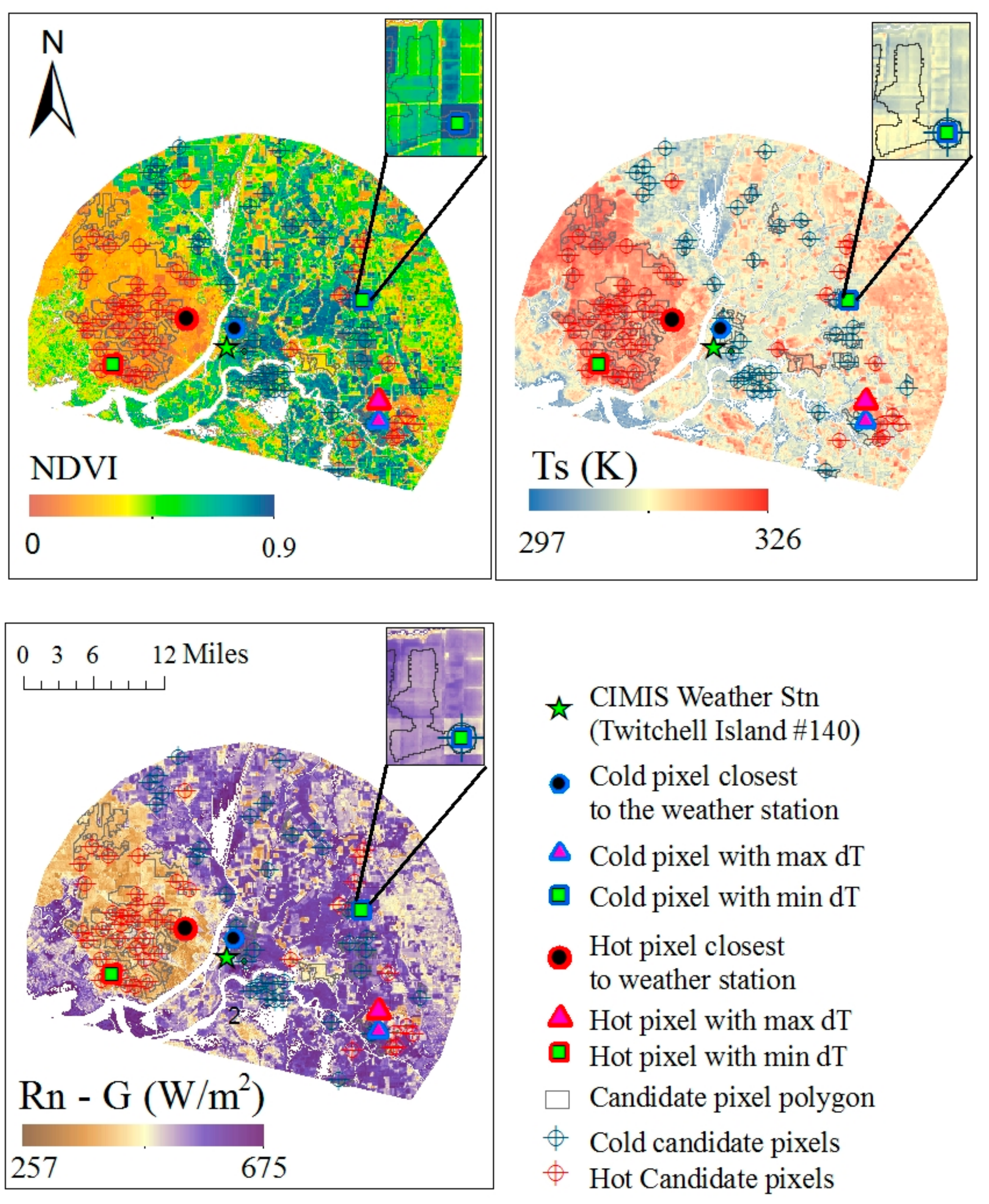
The location of these sets of calibration pixels from 24 July 2014 is presented in Figure 6, along with the spatial distribution of NDVI, Ts, and available energy (Rn − G). From this figure, it can be observed that the image has two distinct regions—a region with less vegetation, higher surface temperature, and lower available energy (eastern side) and another region with more vegetation, lower surface temperature, and higher available energy (western side). However, rather than being concentrated in only these two regions, hot and cold pixels are scattered across the study area. In some instances, where clouds were not filtered correctly, cold candidate pixels were sometimes concentrated in areas with clouds and shadows due to lower temperatures around the area. So, each candidate pixel selection result needs to be manually checked for such errors.
With the automated pixel selection process, there were a total of 47 hot and 38 cold candidate pixels selected for this day. Manual inspection of these pixels in NDVI, RGB, and Ts images as suggested by Allen et al. [19] and Bhattarai et al. [18] indicated that any of them could feasibly be considered an anchor end-member pixel for calibration. That selection would depend subjectively on the modeler.
3.2. Effect of Calibration Pixel Selection on ET
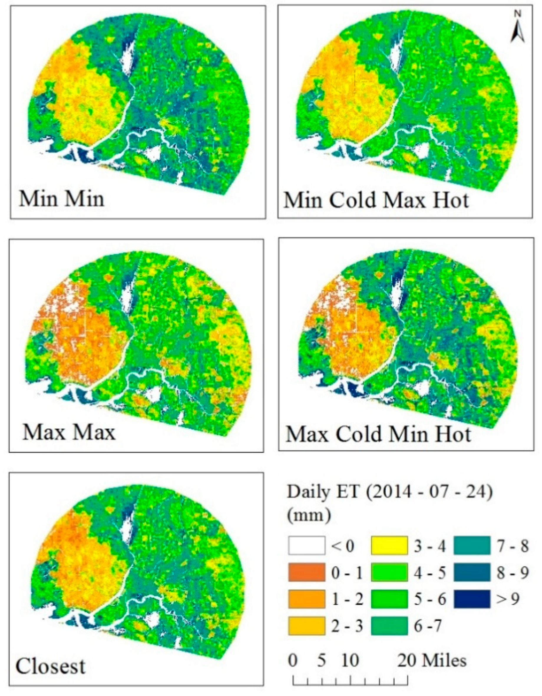
The effect of selecting various calibration pixel sets on ET within the study area was evident as shown by the variability in ET in Figure 7 and Figure 8. Figure 7 illustrates the spatial variability in daily ET computed using the sets of calibration pixels for a specific date, while Figure 8 illustrates the frequency distribution of these ET values. Together, these figures show that, in the study area, highest ET resulted from the Min Min set (5.8 mm) and lowest ET resulted from the Max Max set (4.5 mm). This was an expected result since the Min Min set calibrates using a low dT value, which would provide lower H values and, thus, higher LE and ET values. Similarly, the Max Max set calibrates using higher dT, which would provide higher H values and, thus, lower LE and ET values. The highest variability was in the Max Cold Min Hot set with a standard deviation of 2.5 mm, while the least variability was in the Min Cold Max Hot set with standard deviation of 1.8 mm.
The frequency distribution of these ET maps, along with their means and standard deviations, is presented in Figure 8. The least variability is observed when the model was calibrated using the Min Cold Max Hot set with a standard deviation of 1.8 mm, while the highest variability is observed when the calibration was done using the Max Cold Min Hot set with a standard deviation of 2.5 mm. The peaks for the Max Max set and the Min Cold Max Hot set occur at approximately 6.5 mm while the peaks for the Min Min set and the Max Cold Min Hot set occur at approximately 7.5 mm. ET distributions do not have a discernable scaling or skewing factor according to the calibration sets.
The range of variability in ET due to calibration pixel selection can be seen through the coefficient of variation of mean ET values (4% to 20%) computed using different calibration sets, as illustrated in Figure 9. This figure also shows that variation in ET due to calibration pixel selection is not affected by antecedent moisture conditions due to rainfall, but variability in ET due to calibration does have an increasing trend with time within the growing season. This increase in the coefficient of variation could possibly be attributed to higher variability in lower ET values later in the growing season (Figure 9 and Figure 10).
3.3. Evaluation of Daily ET Estimates from Different Calibration Sets
Comparisons of modeled results with ET estimated at the flux tower are presented in Table 3 and Figure 10. We selected daily ET for validation since daily values are considered to be more useful than instantaneous ET, especially for agricultural applications [16]. Additionally, diurnal storage of heat averages out over daily time scales, which causes better energy balance closure and thus provides better estimates of ET [51]. The closest set results reflect what the values would be if the anchor pixel were selected using the traditional method, closest to the weather station, as suggested by Allen et al. [19] and Bhattarai et al. [18]. Additional results from Table 3 indicate that although r2 is similar for all the sets for each year, ET computed using the cold pixel that provided the minimum dT and the hot pixel that provided the maximum dT (the Min Cold Max Hot set) performed the best, with higher NSE, lower RMSE, and lower Pbias. For the results of 2015, the Min Min set performed as well as the Min Cold Max Hot set. The worst set for calibration was the Max Max set, which had lower r2, lower NSE, higher RMSE, and higher Pbias values. These results also indicate that METRIC overall underestimated ET, resulting in negative biases for most cases.
At any date in the time series, the difference in ET between the flux tower value and ET from any of the calibration sets was no more than ~70% (Figure 10), showing that the temporal pattern of ET is well captured when using any of the calibration sets for computation of ET. The temporal pattern was better captured for 2013 and 2015 with higher NSE values than 2014.
4. Discussion
4.1. Candidate Calibration Pixel Properties
The variability in ET computed using different sets of anchor pixel pairs shows that there are properties of candidate calibration pixels that cannot be completely quantified using only NDVI and Ts. As the candidate pixels have very low variability in Ts for a consistent ET result across the study area regardless of which candidate pixel pair is chosen, it was expected that the iterative calibration process would converge to the same dT. Based on suggestions in previous studies, H could be expected to absorb the biases introduced at earlier steps of the model run. However, our results indicate that not all candidate pixel pairs converge to the same dT, and the differences in dT at these pixel locations are large enough to have a significant effect on final ET results. Furthermore, calibration of the model using a specific dT vs. Ts (Min Cold Max Hot) relation provided consistently better results across multiple years despite little variation in Ts, and dT values coincide closely with available energy. Therefore, it can be presumed that the large differences in dT among the candidate pixels were not random noise, and that the inclusion of available energy into the calibration pixel selection process could potentially improve the calibration process and provide better estimates of ET.
When comparing properties of candidate pixels, we see that cold pixel sets have lower variability compared to the hot pixel set, which can be explained by the properties of the study area and the nature of these extreme pixels. Cold pixels are more readily available than hot pixels because it is easier to find well-watered agricultural pixels in a region having large areas of irrigated agriculture, since these have a relatively consistent set of surface conditions. Hot pixels, on the other hand, lie within dry, bare agricultural areas with higher Ts, and can have more varied surface conditions [21]. The higher variability in surface properties of hot candidate pixels leads to higher variability in dT.
The automated calibration processes in previous studies [18,19,21] have used a specific property of pixels (surface temperature or Ts) to evaluate the performance of the candidate pixel selection process. However, our study shows that evaluating the automated calibration process using temperature might not be useful because of the small variation in Ts between candidate pixels. While the evaluation performed by Bhattarai et al. [18] did compare daily ET to EC flux tower data, the final anchor pixel selection in their work was based on a temperature window of 0.25 K with an NDVI window of 0.01 from which the closest pixel to weather station was chosen. Based on our analysis, these temperature and NDVI windows are comparable to the variability within candidate pixels, meaning that ET variability would not be reduced. As an example, in Figure 5, NDVI variability ranges between 0.05 and 0.07 while Ts variability ranges between 0.1 K and 0.4 K for cold and hot pixels, respectively. This shows that ET computed with any pixels in the windows specified by Bhattarai et al. [18] should have similar variability in ET as that shown in our work.
A surface property that affects the calibration process is the actual weather station surface roughness. Any application of METRIC using past weather data requires us to estimate the surface roughness of the weather station using remote sensing data. Given the wind speed at a specific known height and an assumed logarithmic wind profile, this surface roughness is used to approximate the wind speed at a height 200 m above the ground surface. This predicted wind speed is considered to be constant throughout the image. Any error in this extrapolation can lead to error in the calibration process and final ET results.
4.2. Model Performance
Other studies have attempted to investigate the variation in the end-member pixel’s impact on model accuracy [21,50]. These studies explain that by selecting pixels that have increased (or decreased) temperature of hot and cold extremes together, the values of evaporative fraction (EF) increase (or decrease) with similar impact. These studies also explain that varying end-members should not substantially affect the standard deviation of EF frequency distribution. Yet, as shown in our study, there were differences not only in total ET, but also in standard deviation when end-members were varied. Since METRIC’s performance depends strongly on candidate pixel selection, one would expect differences in model performance with the five calibration pixel sets, and this is indeed what we observe.
Higher ET values are expected at the lower end of the distribution when calibrated using a cold pixel with minimum dT and lower ET values are expected at the higher end of the distribution when calibrated using a hot pixel with maximum dT. However, ET values can vary around the center of the distribution without discernable differences among results from various calibration sets.
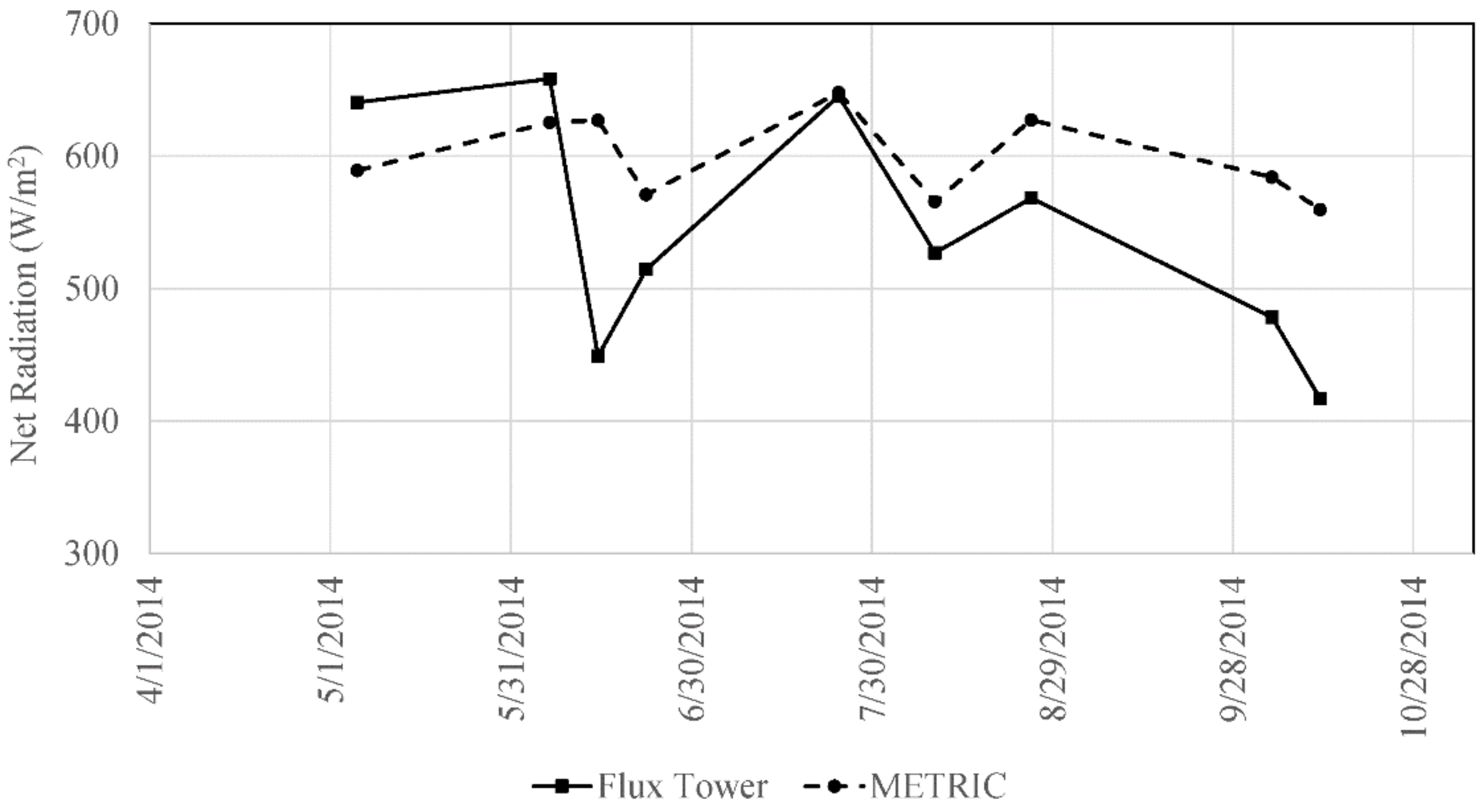
As shown in the results, the model’s performance varied not only with calibration pixel selection, but also with the analysis year. The poor performance of the model for 2014 could be due to the error involved with estimating net solar radiation in METRIC, which was inspected using flux tower data (Figure 11). Other models (e.g., SEBAL or Two Source Energy Balance) which use evaporative fraction (EF) as the ratio of instantaneous LE to available energy (Rn − G) to compute daily ET might perform better for conditions when the estimation of net radiation has larger biases. This effect can be seen in Figure 12, which shows a comparison between instantaneous and daily EF and ETrF values computed using flux tower energy balance components. The higher r2 value for ETrF than EF (between instantaneous and daily measurements) shows that instantaneous values of energy balance components transfer more consistently to daily scales when using ETrF. Consequently, the daily values of ET are more sensitive to errors in instantaneous values. Gonzalez-Dugo et al. [52] also showed that for models other than METRIC, use of EF improved the performance of the models as measured by reduction of the root-mean-squared error and increases in r2 when compared to ETrF. However, we expect that METRIC, although it does not use EF, performs better for most other cases since it uses ETrF, which can capture advection. Significantly higher precipitation in 2014 than in the other years (Figure 9 and Figure 13) provides another possible explanation for the poor model performance that year. This might have caused the adjustment offset (Tfac, which is subtracted from Ts when selecting the hot pixel) to be erroneous since the relation used for Tfac in our work was developed for a drier location in Southern Idaho during 2000.
4.3. Use and Limitations of This Approach to Estimate Variability in METRIC Due to Calibration Pixel Selection
The results obtained here suggest that there can be substantial variation in ET values within calibration pixels when following the techniques outlined in Allen et al. [19]. The process outlined in our work provides a simple method to estimate variability associated with model calibration. It can now be more readily used by less experienced users since it requires much less expert intervention and can allow for quicker analysis using an automated setting. These factors enable its use to compute ET on an operational basis. Although the computational requirement might be higher with multiple results of each individual imagery, using a cloud-based platform such as Google Earth Engine significantly reduces the computational time and storage required.
There are some issues inherent to METRIC that remain challenges for successful application of the approach. Naturally, the results can only be as good as the model inputs. Another major issue during the calibration process remains accurately identifying clouds, shadows, and agricultural lands. Cloud effects were particularly evident when selecting cold pixels, though filtering the clouds through a 7 × 7 filter helped avoid inaccurate identification of cold pixels close to the clouds. Overall, the F-mask algorithm [26] identified clouds in most images, but some images still needed visual inspection to identify and delineate the clouds.
Since each pixel property is important for calibration, the accuracy of the final ET results is highly dependent on accurate agricultural area selection. Although we used USGS National Land Cover Database (NLCD) 2011 agricultural land data for calibration pixel selection, various classification algorithms can be used to first identify land cover types then use the classified land cover for calibration of the model if no land use data is available.
Calibration of METRIC needs a range of pixels having a wide range of evaporative stresses and assumes that there are areas of dry and of wet pixels. Using the approach outlined, different sets of calibration pixels could be used for different climactic and ground conditions. As an example, if the study area received high precipitation, a calibration relationship with lower dT values might perform better owing to the lowered sensible heat flux.
An appropriate area selection for model calibration is important so that the calibration relation of dT vs. Ts remains linear. The area should have contrasting hydrologic regions (with highly irrigated and very dry areas), stable weather conditions, and relatively unchanging topography. For regions that do not have well-irrigated fields, researchers [50] have suggested using water bodies for selection of a cold calibration pixel. However, since the storage term in the energy balance formulation could have higher uncertainties, extra precaution and further study is needed prior to selecting a water body as the cold pixel.
Most major limitations of this study are the ones within METRIC. There are other sources of errors beyond calibration pixel selection, though Allen et al. [17] iterate that accurate calibration can reduce biases and errors in model. However, since there is no easy, specific method for identifying the accuracy of the calibration process, we assume that the calibration process reduced biases due to parameter selection in empirical relations used prior to calibration.
5. Conclusions
This study aimed to provide an approach for measuring the variability of watershed-scale ET estimates induced by human intervention in the calibration process. To do so, we examined the effect of anchor pixels on the performance of a satellite-based remote sensing ET model, METRIC. Differences resulting from anchor pixel set selection were shown to cause markedly different ET results, and we showed that including available energy when selecting a candidate pixel could improve the performance of the model. Based on this analysis, we demonstrate that the differences in ET, due to selection of a set of anchor pixels after the automatic selection process, of candidate pixels can range between 5% and 20%, based on the coefficient of variation. When compared to ET measurements from an eddy flux tower, the model’s overall performance was best when the selected cold pixel had the minimum dT and the selected hot pixel had the maximum dT (from among all candidate pixels). Using these cold and hot pixels, ET results were more accurate than when using the traditional method of selecting a set of anchor pixels closest to the weather station (again from within a pool of calibration pixels). With an increasing volume of satellite image products, it can be expected that the use of models like METRIC will expand from roles as merely investigative research tools to serving as operational models for short-term and long-term decision-making. Our work aids in this transition by helping extend the domain of the model from well-trained modelers and experts to inexperienced and new users by providing a measure of uncertainty associated with the results. Models like METRIC must be calibrated for each specific image and being able to calibrate expediently is therefore crucial. With our study, a variability measure corresponding to selected calibration pixels around a specific weather station is easier to automate. Since our method of calibration does not strictly depend on closeness to a weather station, it can be more applicable for automating calibration of METRIC than the method outlined by Allen et al. [19] for cases when the reference weather station is not present within the image. It also provides a range of ET results that can be incorporated into uncertainty measures. Together, these will ultimately allow better water resources planning and management decisions.
Data Statement:
All raster data used in this study were obtained using from the GEE catalog and its functions. Use of GEE and its catalog requires creating an account with Google. The catalog provides a short description of the image, the bands available, and metadata or properties of the image. Images or raster data are provided as Image collections. For our work we used the following collections:
Data extraction and use:
We present an example (using JavaScript in Earth Engine Code Editor at https://code.earthengine.google.com) which shows how to obtain NDVI for a Landsat 8 image using the GEE catalog and functionalities.
- // Load a Landsat 8 ImageCollection for a single path-row.
- var collection = ee.ImageCollection(‘LANDSAT/LC08/C01/T1_TOA’)
- .filter(ee.Filter.eq(‘WRS_PATH’, 44))
- .filter(ee.Filter.eq(‘WRS_ROW’, 34))
- .filterDate(‘2015-06-25’, ‘2015-07-01’);
- // Get the first image from the image collection
- var img = ee.Image(collection.first());
- // Define a function to compute NDVI.
- var NDVI = function(image) {
- return image.expression(‘float(b(“B5”) − b(“B4”)) / (b(“B5”) + b(“B4”))’);
- };
- // Use NDVI function
- NDVI_img = NDVI(img);
- // Display the NDVI image
- Map.addLayer (NDVI_img, {min: 0, max: 1, palette: ‘red, yellow, green’}, ‘NDVI’);
Supplementary Materials
Supplementary materials can be found at https://www.mdpi.com/2072-4292/10/11/1695/s1, Figure S1: Distribution of SAVI values for hot and cold candidate pixels.
Author Contributions
Conceptualization: S.D. and M.E.B. Methodology: S.D. Software: S.D. Validation: S.D. Formal Analysis: S.D. Investigation: S.D. and M.E.B. Resources: M.E.B. Data Curation: S.D. Writing—Original Draft preparation: S.D. Writing—Review and Editing: M.E.B. Visualization: S.D. Supervision: M.E.B. Project Administration: M.E.B. Funding Acquisition: M.E.B.
Funding
This research was funded by Washington State Department of Ecology, Office of Columbia River.
Acknowledgments
This study is based on the work supported by Washington State Department of Ecology, Office of Columbia River. The authors would also like to thank US-AmeriFlux and Dennis Baldocchi at University of California Berkley for providing ET/Flux data measurements to the public. The authors would also like to express a sincere thank you to Mason Kreidler for providing constructive criticism of the manuscript.
Conflicts of Interest
The authors declare no conflict of interest.
References
- Wang, K.; Dickinson, R.E. A review of global terrestrial evapotranspiration: Observation, modeling, climatology, and climatic variability. Rev. Geophys. 2012, 50, 1–54. [Google Scholar] [CrossRef]
- Wallace, J.S. Increasing agricultural water use efficiency to meet future food production. Agric. Ecosyst. Environ. 2000, 82, 105–119. [Google Scholar] [CrossRef]
- Farahani, H.J.; Howell, T.A.; Shuttleworth, W.J.; Bausch, W.C. Evapotranspiration: Progress in measurement and modeling in agriculture. Trans. ASABE 2007, 50, 1627–1638. [Google Scholar] [CrossRef]
- Verstraeten, W.; Veroustraete, F.; Feyen, J. Assessment of evapotranspiration and soil moisture content across different scales of observation. Sensors 2008, 8, 70–117. [Google Scholar] [CrossRef] [PubMed]
- Dugas, W.A.; Upchurch, D.R.; Ritchie, J.T. A weighing lysimeter for evapotranspiration and root measurements. Agron. J. 1985, 77, 821–825. [Google Scholar] [CrossRef]
- Aubinet, M.; Vesala, T.; Papale, D. Eddy Covariance a Practical Guide to Measurement and Data Analysis; Springer: Dordrecht, The Netherlands; New York, NY, USA, 2012; pp. 59–82. ISBN 978-94-007-2351-1. [Google Scholar]
- Ezzahar, J.; Chehbouni, A.; Hoedjes, J.C.B.; Er-Raki, S.; Chehbouni, A.; Boulet, G.; Bonnefond, J.M.; De Bruin, H.A.R. The use of the scintillation technique for monitoring seasonal water consumption of olive orchards in a semi-arid region. Agric. Water Manag. 2007, 89, 173–184. [Google Scholar] [CrossRef] [Green Version]
- Meiresonne, L.; Nadezhdin, N.; Cermak, J.; Van Slycken, J.; Ceulemans, R. Measured sap flow and simulated transpiration from a poplar stand in Flanders (Belgium). Agric. For. Meteorol. 1999, 96, 165–179. [Google Scholar] [CrossRef]
- Billah, M.M.; Goodall, J.L.; Narayan, U.; Reager, J.T.; Lakshmi, V.; Famiglietti, J.S. A methodology for evaluating evapotranspiration estimates at the watershed-scale using GRACE. J. Hydrol. 2015, 523, 574–586. [Google Scholar] [CrossRef] [Green Version]
- Allen, R.G.; Pereira, L.S.; Raes, D.; Smith, M. Crop Evapotranspiration-Guidelines for Computing Crop Water Requirements; FAO: Rome, Italy, 1998; pp. 87–101. ISBN 92-5-104219-5. [Google Scholar]
- Godfray, H.C.J.; Beddington, J.R.; Crute, I.R.; Haddad, L.; Lawrence, D.; Muir, J.F.; Pretty, J.; Robinson, S.; Thomas, S.M.; Toulmin, C. Food security: The challenge of feeding 9 billion people. Science 2010, 327, 812–818. [Google Scholar] [CrossRef] [PubMed]
- Bastiaanssen, W.G.M.; Noordman, E.J.M.; Pelgrum, H.; Davids, G.; Thoreson, B.P.; Allen, R. SEBAL model with remotely sensed data to improve water-resources management under actual field conditions. J. Irrig. Drain. Eng. 2005, 131, 85–93. [Google Scholar] [CrossRef]
- Bayat, B.; van der Tol, C.; Verhoef, W. Integrating satellite optical and thermal infrared observations for improving daily ecosystem functioning estimations during a drought episode. Remote Sens. Environ. 2018, 209, 375–394. [Google Scholar] [CrossRef]
- Chance, E.; Cobourn, K.; Thomas, V. Trend detection for the extent of irrigated agriculture in Idaho’s Snake river plain, 1984–2016. Remote Sens. 2018, 10, 145. [Google Scholar] [CrossRef]
- Liou, Y.-A.; Kar, S. Evapotranspiration estimation with remote sensing and various surface energy balance algorithms: A review. Energies 2014, 7, 2821. [Google Scholar] [CrossRef]
- Allen, R.G.; Tasumi, M.; Trezza, R. Satellite-based energy balance for mapping evapotranspiration with internalized calibration (METRIC)—Model. J. Irrig. Drain. Eng. 2007, 133, 380–394. [Google Scholar] [CrossRef]
- Allen, R.; Irmak, A.; Trezza, R.; Hendrickx, J.M.H.; Bastiaanssen, W.; Kjaersgaard, J. Satellite-based ET estimation in agriculture using SEBAL and METRIC. Hydrol. Process. 2011, 25, 4011–4027. [Google Scholar] [CrossRef]
- Bhattarai, N.; Quackenbush, L.J.; Im, J.; Shaw, S.B. A new optimized algorithm for automating endmember pixel selection in the SEBAL and METRIC models. Remote Sens. Environ. 2017, 196, 178–192. [Google Scholar] [CrossRef]
- Allen, R.G.; Burnett, B.; Kramber, W.; Huntington, J.; Kjaersgaard, J.; Kilic, A.; Kelly, C.; Trezza, R. Automated calibration of the METRIC-Landsat evapotranspiration process. JAWRA J. Am. Water Resour. Assoc. 2013, 49, 563–576. [Google Scholar] [CrossRef]
- Bhattarai, N.; Shaw, S.B.; Quackenbush, L.J.; Im, J.; Niraula, R. Evaluating five remote sensing based single-source surface energy balance models for estimating daily evapotranspiration in a humid subtropical climate. Int. J. Appl. Earth Obs. Geoinf. 2016, 49, 75–86. [Google Scholar] [CrossRef]
- Morton, C.G.; Huntington, J.L.; Pohll, G.M.; Allen, R.G.; McGwire, K.C.; Bassett, S.D. Assessing calibration uncertainty and automation for estimating evapotranspiration from agricultural areas using METRIC. JAWRA J. Am. Water Resour. Assoc. 2013, 49, 549–562. [Google Scholar] [CrossRef]
- Eichelmann, E.; Hemes, K.S.; Knox, S.H.; Oikawa, P.Y.; Chamberlain, S.D.; Sturtevant, C.; Verfaillie, J.; Baldocchi, D.D. The effect of land cover type and structure on evapotranspiration from agricultural and wetland sites in the Sacramento–San Joaquin River Delta, California. Agric. For. Meteorol. 2018, 256–257, 179–195. [Google Scholar] [CrossRef]
- Oikawa, P.Y.; Sturtevant, C.; Knox, S.H.; Verfaillie, J.; Huang, Y.W.; Baldocchi, D.D. Revisiting the partitioning of net ecosystem exchange of CO2 into photosynthesis and respiration with simultaneous flux measurements of 13CO2 and CO2, soil respiration and a biophysical model, CANVEG. Agric. For. Meteorol. 2017, 234–235, 149–163. [Google Scholar] [CrossRef]
- Stannard, D.I. Comparison of Penman-Monteith, Shuttleworth-Wallace, and modified Priestley-Taylor evapotranspiration models for wildland vegetation in semiarid rangeland. Water Resour. Res. 1993, 29, 1379–1392. [Google Scholar] [CrossRef]
- Kilic, A.; Allen, R.; Trezza, R.; Ratcliffe, I.; Kamble, B.; Robison, C.; Ozturk, D. Sensitivity of evapotranspiration retrievals from the METRIC processing algorithm to improved radiometric resolution of Landsat 8 thermal data and to calibration bias in Landsat 7 and 8 surface temperature. Remote Sens. Environ. 2016, 185, 198–209. [Google Scholar] [CrossRef]
- Foga, S.; Scaramuzza, P.L.; Guo, S.; Zhu, Z.; Dilley, R.D.; Beckmann, T.; Schmidt, G.L.; Dwyer, J.L.; Joseph Hughes, M.; Laue, B. Cloud detection algorithm comparison and validation for operational Landsat data products. Remote Sens. Environ. 2017, 194, 379–390. [Google Scholar] [CrossRef] [Green Version]
- Gorelick, N.; Hancher, M.; Dixon, M.; Ilyushchenko, S.; Thau, D.; Moore, R. Google Earth Engine: Planetary-scale geospatial analysis for everyone. Remote Sens. Environ. 2017, 202, 18–27. [Google Scholar] [CrossRef]
- Ke, Y.; Im, J.; Park, S.; Gong, H. Downscaling of MODIS one kilometer evapotranspiration using Landsat-8 data and machine learning approaches. Remote Sens. 2016, 8, 215. [Google Scholar] [CrossRef]
- Tasumi, M.; Allen, R.G.; Trezza, R. At-surface reflectance and albedo from satellite for operational calculation of land surface energy balance. J. Hydrol. Eng. 2008, 13, 51–63. [Google Scholar] [CrossRef]
- Liang, S. Narrowband to broadband conversions of land surface albedo I: Algorithms. Remote Sens. Environ. 2001, 76, 213–238. [Google Scholar] [CrossRef]
- Sobrino, J.A.; Jiménez-Muñoz, J.C.; Paolini, L. Land surface temperature retrieval from LANDSAT TM 5. Remote Sens. Environ. 2004, 90, 434–440. [Google Scholar] [CrossRef]
- Jimenez-Munoz, J.C.; Cristobal, J.; Sobrino, J.A.; Soria, G.; Ninyerola, M.; Pons, X. Revision of the single-channel algorithm for land surface temperature retrieval from Landsat thermal-infrared data. IEEE Trans. Geosci. Remote Sens. 2009, 47, 339–349. [Google Scholar] [CrossRef]
- Yu, X.; Guo, X.; Wu, Z. Land surface temperature retrieval from Landsat 8 TIRS—Comparison between radiative transfer equation-based method, split window algorithm and single channel method. Remote Sens. 2014, 6, 9829. [Google Scholar] [CrossRef]
- Zanter, K. Landsat 8 (L8) Data Users Handbook. Available online: https://landsat.usgs.gov/sites/default/files/documents/LSDS-1574_L8_Data_Users_Handbook.pdf (accessed on 6 June 2018).
- Bastiaanssen, W.G.M.; Menenti, M.; Feddes, R.A.; Holtslag, A.A.M. A remote sensing surface energy balance algorithm for land (SEBAL): Part 1. Formulation. J. Hydrol. 1998, 212–213, 198–212. [Google Scholar] [CrossRef]
- Bastiaanssen, W.G.M.; Pelgrum, H.; Wang, J.; Ma, Y.; Moreno, J.F.; Roerink, G.J.; van der Wal, T. A remote sensing surface energy balance algorithm for land (SEBAL): Part 2: Validation. J. Hydrol. 1998, 212–213, 213–229. [Google Scholar] [CrossRef]
- Businger, J.A.; Wyngaard, J.C.; Izumi, Y.; Bradley, E.F. Flux-profile relationships in the atmospheric surface layer. J. Atmos. Sci. 1971, 28, 181–189. [Google Scholar] [CrossRef]
- Brutsaert, W. Evaporation. In Hydrology: An Introduction; Brutsaert, W., Ed.; Cambridge University Press: Cambridge, UK, 2005; pp. 117–158. ISBN 9780521824798. [Google Scholar]
- Bastiaanssen, W.G.M. Regionalization of Surface Flux Densities and Moisture Indicators in Composite Terrain: A Remote Sensing Approach under Clear Skies in Mediterranean Climates. PhD Thesis, Wageningen Agricultural University, Wageningen, The Netherlands, 1995. [Google Scholar]
- Allen, R.G.; Morton, C.; Kamble, B.; Kilic, A.; Huntington, J.; Thau, D.; Gorelick, N.; Erickson, T.; Moore, R.; Trezza, R. EEFlux: A Landsat-based evapotranspiration mapping tool on the Google Earth Engine. In Proceedings of the Joint ASABE/IA Irrigation Symposium 2015: Emerging Technologies for Sustainable Irrigation, Long Beach, CA, USA, 10–12 November 2015. [Google Scholar]
- Allen, R.G.; Trezza, R.; Kilic, A.; Tasumi, M.; Li, H. Sensitivity of Landsat-scale energy balance to aerodynamic variability in mountains and complex terrain. JAWRA J. Am. Water Resour. Assoc. 2013, 49, 592–604. [Google Scholar] [CrossRef]
- Irmak, A.; Ratcliffe, I.; Ranade, P.; Hubbard, K.G.; Singh, R.K.; Kamble, B.; Kjaersgaard, J. Estimation of land surface evapotranspiration with a satellite remote sensing procedure. Great Plains Res. 2011, 21, 73–88. [Google Scholar]
- Huete, A.R. A soil-adjusted vegetation index (SAVI). Remote Sens. Environ. 1988, 25, 295–309. [Google Scholar] [CrossRef]
- Burnett, B. A Procedure for Estimating Total Evapotranspiration Using Satellite-Based Vegetation Indices with Separate Estimates from Bare Soil. Master’s Thesis, University of Idaho, Moscow, ID, USA, 2007. [Google Scholar]
- Daughtry, C.S.T.; Hunt, E.R.; Doraiswamy, P.C.; McMurtrey, J.E. Remote Sensing the Spatial Distribution of Crop Residues. Agron. J. 2005, 97, 864–871. [Google Scholar] [CrossRef]
- Horton, R.; Bristow, K.L.; Kluitenberg, G.J.; Sauer, T.J. Crop residue effects on surface radiation and energy balance—Review. Theor. Appl. Clim. 1996, 54, 27–37. [Google Scholar] [CrossRef]
- Nash, J.E.; Sutcliffe, J.V. River flow forecasting through conceptual models part I—A discussion of principles. J. Hydrol. 1970, 10, 282–290. [Google Scholar] [CrossRef]
- Yapo, P.O.; Gupta, H.V.; Sorooshian, S. Automatic calibration of conceptual rainfall-runoff models: Sensitivity to calibration data. J. Hydrol. 1996, 181, 23–48. [Google Scholar] [CrossRef]
- Twine, T.E.; Kustas, W.P.; Norman, J.M.; Cook, D.R.; Houser, P.R.; Meyers, T.P.; Prueger, J.H.; Starks, P.J.; Wesely, M.L. Correcting eddy-covariance flux underestimates over a grassland. Agric. For. Meteorol. 2000, 103, 279–300. [Google Scholar] [CrossRef] [Green Version]
- Long, D.; Singh, V.P. Assessing the impact of end-member selection on the accuracy of satellite-based spatial variability models for actual evapotranspiration estimation. Water Resour. Res. 2013, 49, 2601–2618. [Google Scholar] [CrossRef] [Green Version]
- Foken, T. The energy balance closure problem: An overview. Ecol. Appl. 2008, 1351–1367. [Google Scholar] [CrossRef]
- Gonzalez-Dugo, M.P.; Neale, C.M.U.; Mateos, L.; Kustas, W.P.; Prueger, J.H.; Anderson, M.C.; Li, F. A comparison of operational remote sensing-based models for estimating crop evapotranspiration. Agric. For. Meteorol. 2009, 149, 1843–1853. [Google Scholar] [CrossRef]
Figure 1.
Location of study area with AmeriFlux site and nearby California Irrigation Management Irrigation System (CIMIS) weather station in California. A Red Green Blue (RGB) Landsat 8 image for 24 July 2014 is clipped and overlaid over the study area.
Figure 1.
Location of study area with AmeriFlux site and nearby California Irrigation Management Irrigation System (CIMIS) weather station in California. A Red Green Blue (RGB) Landsat 8 image for 24 July 2014 is clipped and overlaid over the study area.
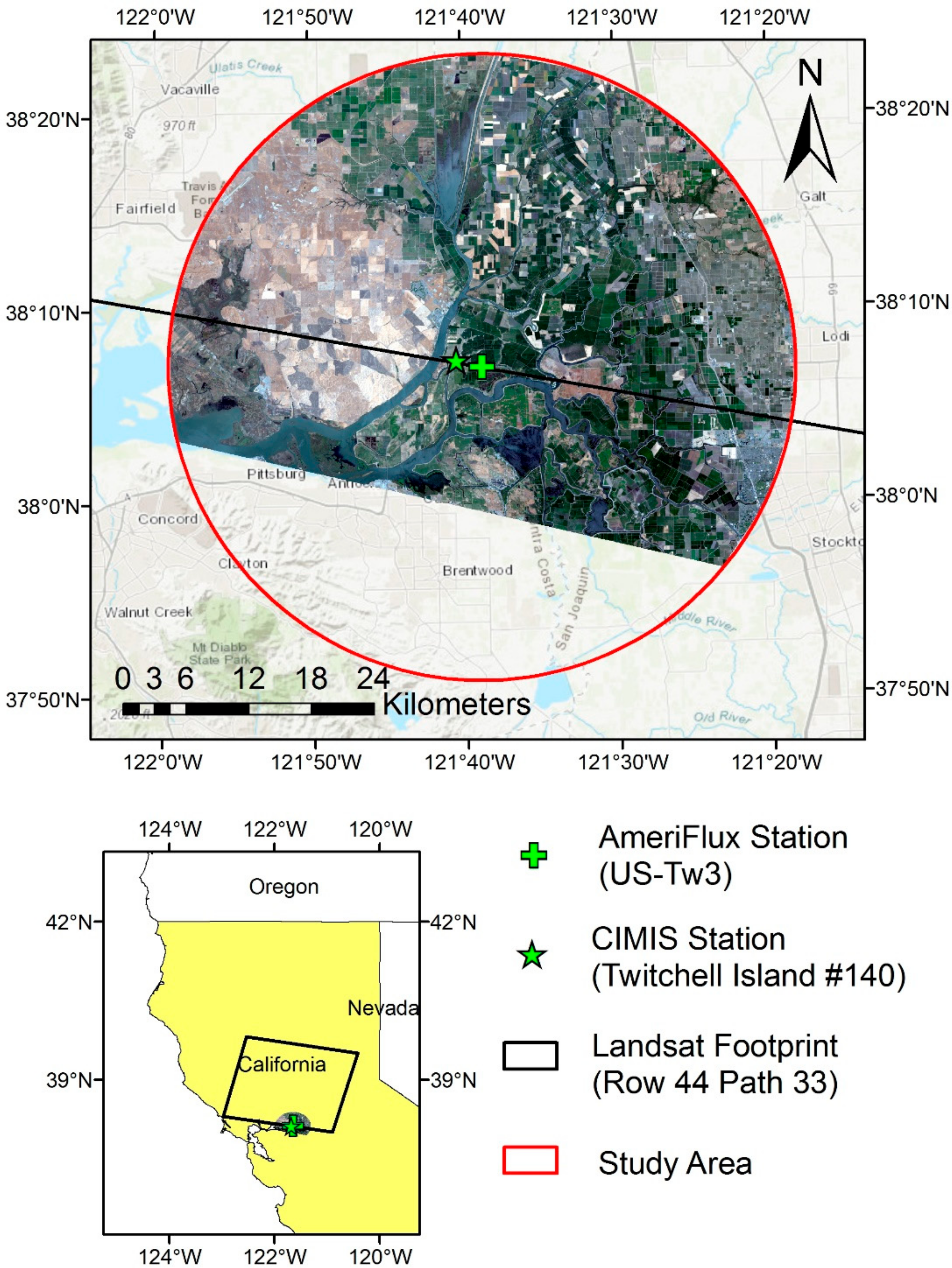
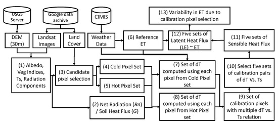
Figure 2.
Methodology for computing variability in Mapping EvapoTranspiration at high Resolution with Internalized Calibration (METRIC) evapotranspiration (ET) due to calibration pixel selection.
Figure 2.
Methodology for computing variability in Mapping EvapoTranspiration at high Resolution with Internalized Calibration (METRIC) evapotranspiration (ET) due to calibration pixel selection.
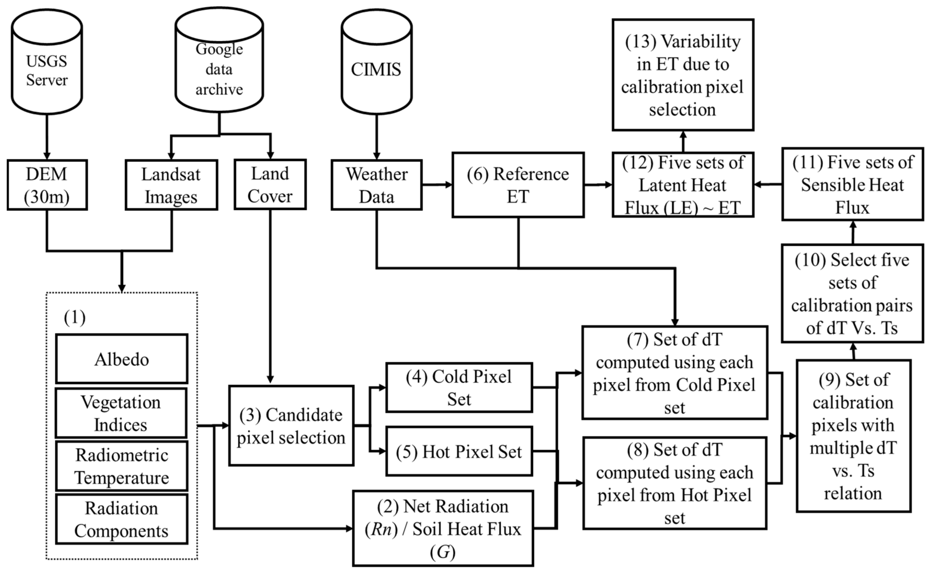
Figure 3.
dT vs. Ts relationship for each candidate hot and cold pixel. Five selected sets are drawn as lines to encompass every possible combination for calibration of the model. (The locations of these points are shown in Figure 6).
Figure 3.
dT vs. Ts relationship for each candidate hot and cold pixel. Five selected sets are drawn as lines to encompass every possible combination for calibration of the model. (The locations of these points are shown in Figure 6).
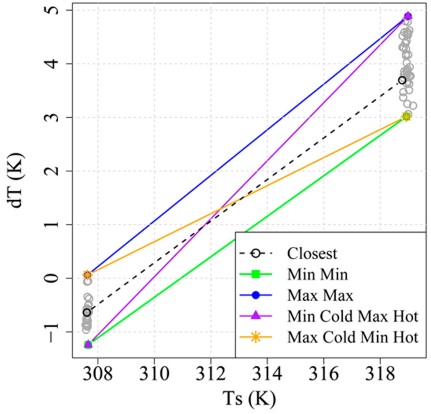
Figure 4.
Coefficient of variation of scaled values of normalized difference vegetation index (NDVI), Ts, and Available Energy for hot (red) and cold (blue) pixels for all images.
Figure 4.
Coefficient of variation of scaled values of normalized difference vegetation index (NDVI), Ts, and Available Energy for hot (red) and cold (blue) pixels for all images.

Figure 5.
Variability in temperature, NDVI, and available energy within candidate anchor pixels for 24-07-2014.
Figure 5.
Variability in temperature, NDVI, and available energy within candidate anchor pixels for 24-07-2014.

Figure 6.
Location of hot and cold calibration pixel sets as polygons (24-07-2014). Inset shows a polygon from which the cold calibration pixel was selected and has minimum dT.
Figure 6.
Location of hot and cold calibration pixel sets as polygons (24-07-2014). Inset shows a polygon from which the cold calibration pixel was selected and has minimum dT.

Figure 7.
Spatial variation in daily ET based on various calibration sets.

Figure 8.
Frequency distribution of ET for different calibration sets for 2014-07-24. The values in the legends are, respectively, [Mean, standard deviation].
Figure 8.
Frequency distribution of ET for different calibration sets for 2014-07-24. The values in the legends are, respectively, [Mean, standard deviation].
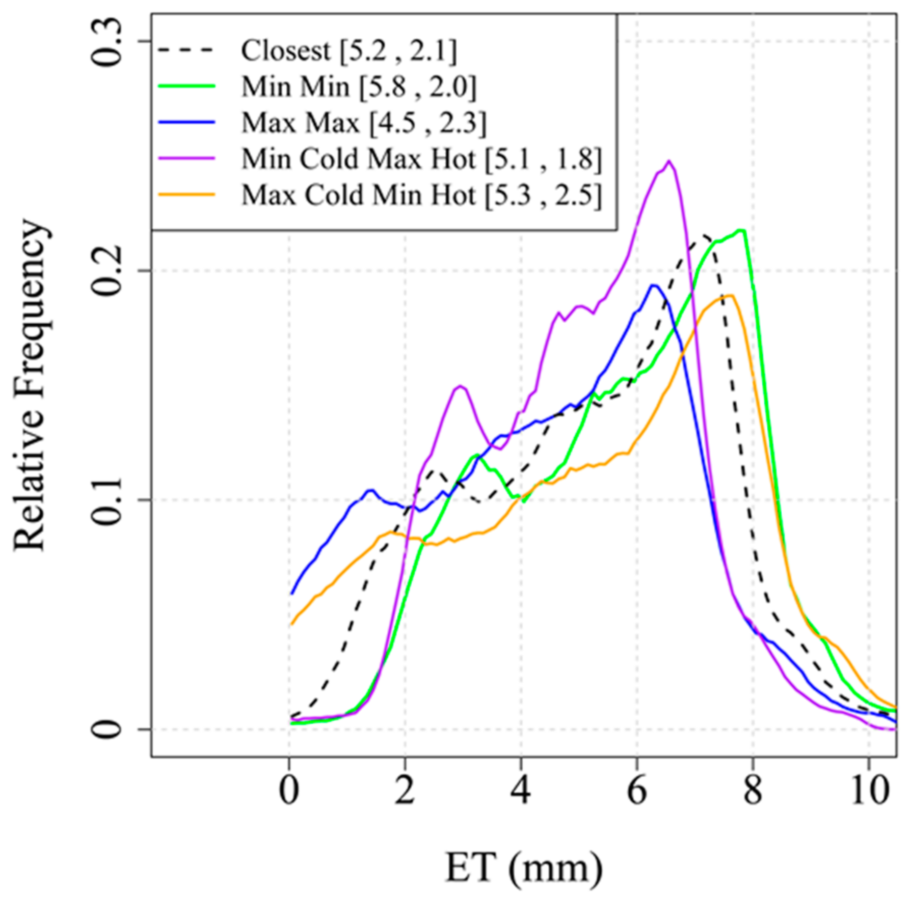
Figure 9.
Coefficient of variation of mean ET calibrated by four sets of calibration pixels (Min Min, Max Max, Min Max, and Max Min). Precipitation added to the plot shows that antecedent moisture conditions did not affect the variability.
Figure 9.
Coefficient of variation of mean ET calibrated by four sets of calibration pixels (Min Min, Max Max, Min Max, and Max Min). Precipitation added to the plot shows that antecedent moisture conditions did not affect the variability.
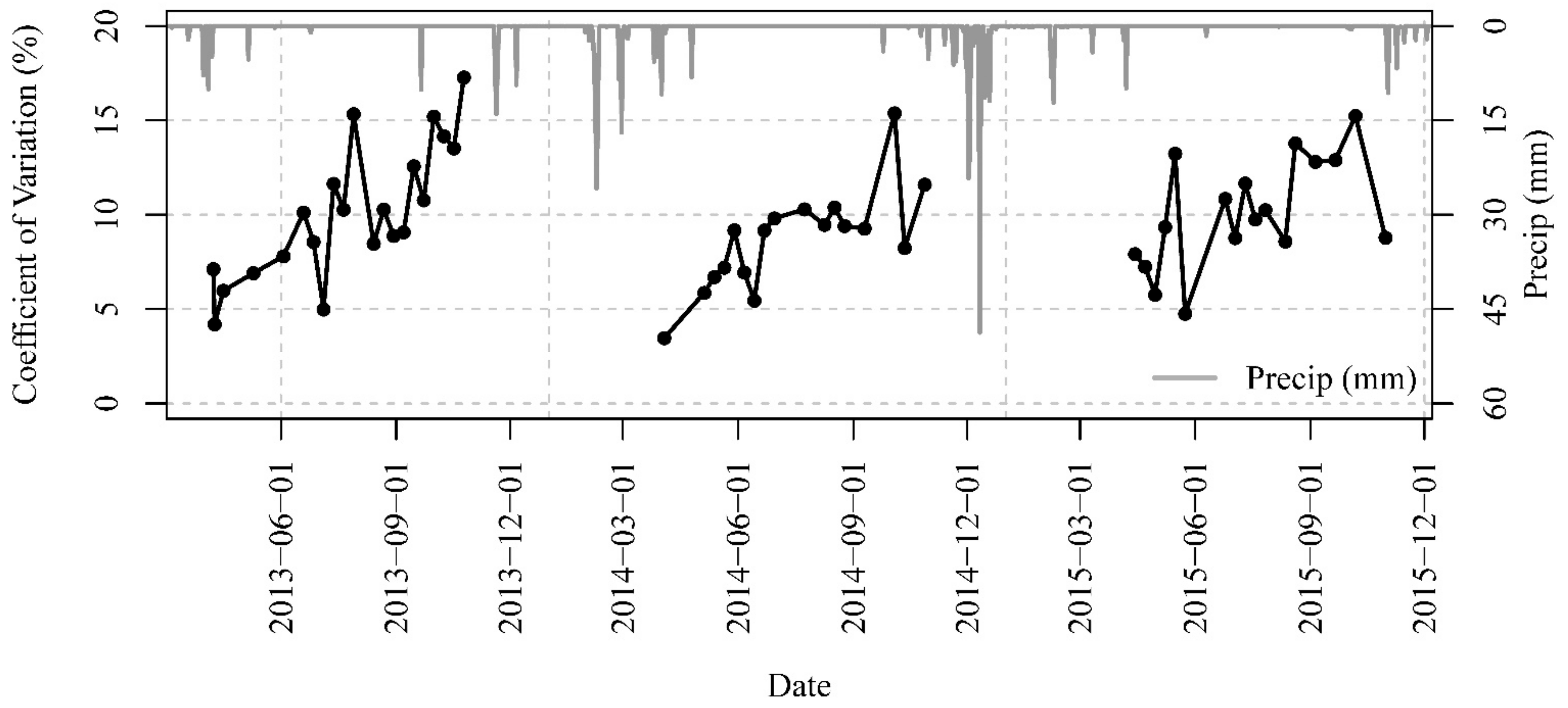
Figure 10.
Comparison of 24-h ET computed using the selected five calibration schemes with eddy covariance flux tower data for 2014, 2015, and 2016. With any of these calibration sets, the temporal pattern of ET over the year is well captured. The line corresponding to “closest” presents results with the traditional method of anchor pixel selection (closest to the weather station).
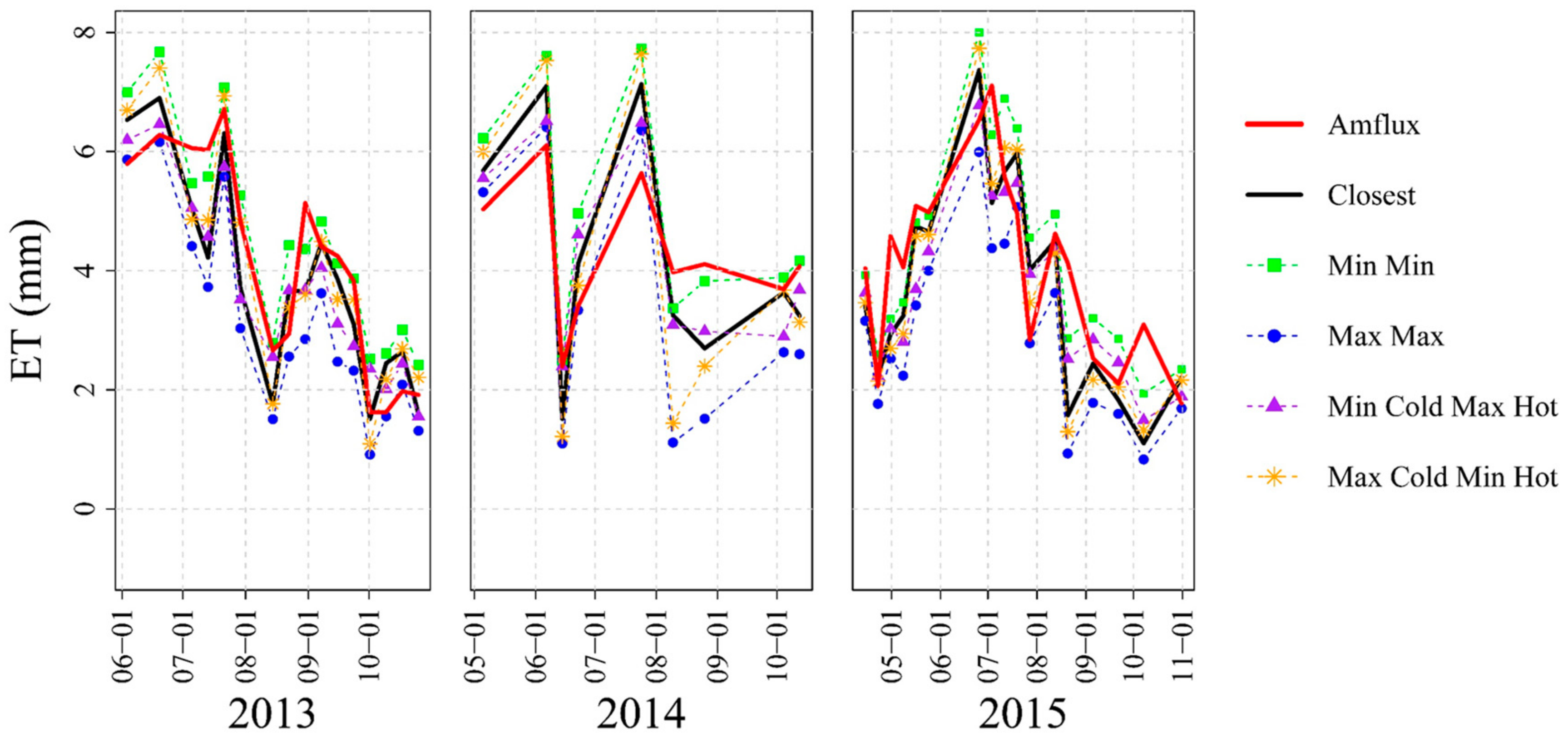
Figure 11.
Validation of net radiation for 2014.

Figure 12.
Comparison between instantaneous and daily Evaporative Fraction (EF) and Reference ET fraction (ETrF) computed using flux tower energy balance components. r2 values are presented in parentheses.
Figure 12.
Comparison between instantaneous and daily Evaporative Fraction (EF) and Reference ET fraction (ETrF) computed using flux tower energy balance components. r2 values are presented in parentheses.
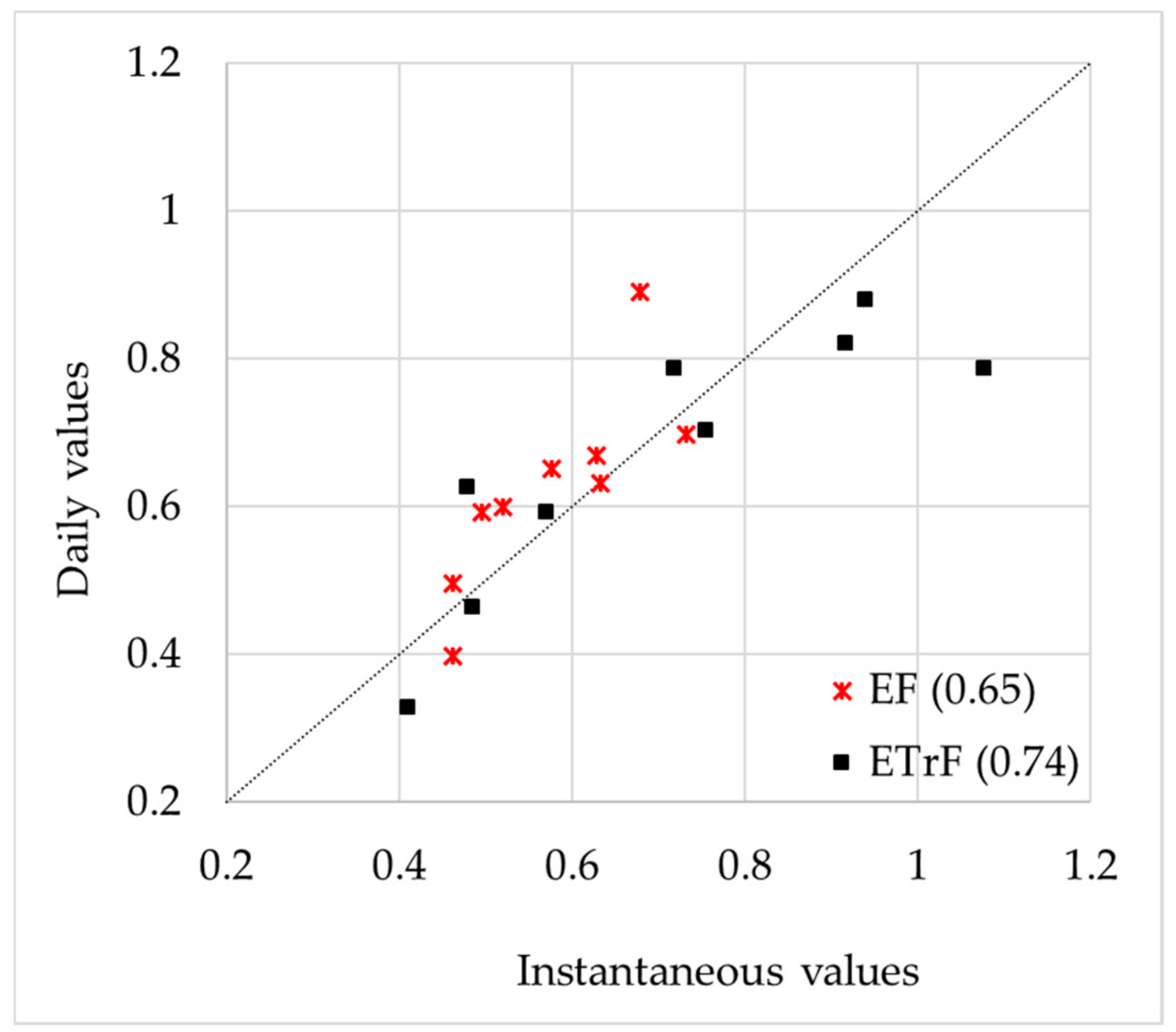
Figure 13.
Total annual precipitation and evapotranspiration for the selected years.


Table 1.
Description of sites used in this study.
| Site Descriptors | Twitchell Island 140 | US-Tw3 |
|---|---|---|
| Latitude (N) | 38.1217 | 38.1159 |
| Longitude (W) | 121.6745 | 121.6467 |
| Elevation (m) | 0 | −9 |
| Cover type | Large Pasture | Alfalfa |
| Data availability period | 1998–current | 2013–2015 |
| Mean Annual temperature (°C) | 15 | 15 |
| Mean Annual precipitation (mm) | 382 | 421 |
| Temporal resolution provided at (min) | 60 | 30 |
| Source of data | CIMIS | Baldocchi 1 |
1 http://dx.doi.org/10.17190/AMF/1246149 (last assessed: 10 Octobe 2017).
Table 2.
List of Landsat images used in this study. Path/row of the image was 044/033.
| YearMonthDay (YYYYMMDD) | Area Cloud Covered (%) | YearMonthDay (YYYYMMDD) | Area Cloud Covered (%) |
|---|---|---|---|
| 2013 | |||
| Landsat 7 | Landsat 8 | ||
| 20130713 | 2% | 20130603 | 5% |
| 20130729 | 4% | 20130619 | 4% |
| 20130814 | 2% | 20130705 | 7% |
| 20130830 | 3% | 20130721 | 7% |
| 20130915 | 3% | 20130822 | 7% |
| 20131001 | 2% | 20130907 | 7% |
| 20131017 | 3% | 20130923 | 7% |
| 20131009 | 7% | ||
| 20131025 | 8% | ||
| 2014 | |||
| Landsat 7 | Landsat 8 | ||
| 20140614 | 4% | 20140505 | 13% |
| 20141004 | 2% | 20140606 | 9% |
| 20140622 | 7% | ||
| 20140724 | 7% | ||
| 20140809 | 7% | ||
| 20140825 | 9% | ||
| 20141012 | 8% | ||
| 2015 | |||
| Landsat 7 | Landsat 8 | ||
| 20150414 | 2% | 20150422 | 8% |
| 20150430 | 2% | 20150508 | 12% |
| 20150516 | 3% | 20150524 | 8% |
| 20150703 | 4% | 20150625 | 8% |
| 20150719 | 5% | 20150711 | 7% |
| 20150820 | 2% | 20150727 | 7% |
| 20150905 | 2% | 20150812 | 7% |
| 20150921 | 3% | 20151031 | 8% |
| 20151007 | 3% | ||
Table 3.
Model evaluation results comparing 24-h ET estimates computed using five different calibration schemes with measured ET at the AmeriFlux eddy covariance (EC) station. (NSE: Nash–Sutcliffe Efficiency, RMSE: Root Mean Squared Error).
Table 3.
Model evaluation results comparing 24-h ET estimates computed using five different calibration schemes with measured ET at the AmeriFlux eddy covariance (EC) station. (NSE: Nash–Sutcliffe Efficiency, RMSE: Root Mean Squared Error).
| r2 | NSE | RMSE (mm) | Pbias (%) | |
|---|---|---|---|---|
| 2013 | ||||
| Closest | 0.78 | 0.75 | 0.87 | −4.0 |
| Min Min | 0.85 | 0.79 | 0.80 | 18.0 |
| Max Max | 0.80 | 0.47 | 1.28 | −25.0 |
| Min Cold Max Hot | 0.80 | 0.75 | 0.88 | −4.0 |
| Max Cold Min Hot | 0.82 | 0.79 | 0.79 | −1.0 |
| 2014 | ||||
| Closest | 0.83 | 0.18 | 0.95 | −7.0 |
| Min Min | 0.81 | 0.04 | 1.03 | 11.0 |
| Max Max | 0.72 | −1.13 | 1.54 | −29.0 |
| Min Cold Max Hot | 0.74 | 0.46 | 0.77 | −4.0 |
| Max Cold Min Hot | 0.77 | −0.82 | 1.42 | −14.0 |
| 2015 | ||||
| Closest | 0.62 | 0.44 | 1.13 | −9.0 |
| Min Min | 0.68 | 0.57 | 0.99 | 8.0 |
| Max Max | 0.63 | 0.01 | 1.50 | −28.0 |
| Min Cold Max Hot | 0.67 | 0.56 | 1.00 | −9.0 |
| Max Cold Min Hot | 0.65 | 0.41 | 1.16 | −10.0 |
| Name | Image Collection ID | Number of Bands |
|---|---|---|
| 1. USGS Landsat 7 Collection 1 Tier 1 Raw Scenes | LANDSAT/LE07/C01/T1 | 10 |
| 2. USGS Landsat 7 Collection 1 Tier 1 top-of-atmosphere (TOA) Reflectance | LANDSAT/LE07/C01/T1_TOA | 10 |
| 3. USGS Landsat 7 Surface Reflectance (SR) Tier 1 | LANDSAT/LE07/C01/T1_SR | 11 |
| 4. USGS Landsat 8 Collection 1 Tier 1 Raw Scenes | LANDSAT/LC08/C01/T1 | 12 |
| 5. USGS Landsat 8 Collection 1 Tier 1 top-of-atmosphere (TOA) Reflectance | LANDSAT/LC08/C01/T1_TOA | 12 |
| 6. USGS Landsat 8 Surface Reflectance Tier 1 | LANDSAT/LC08/C01/T1_SR | 12 |
| 7. USGS National Elevation Dataset 1/3 arc-second | USGS/NED | 1 |
| 8. NLCD: USGS National Land Cover Database | USGS/NLCD | 4 |
© 2018 by the authors. Licensee MDPI, Basel, Switzerland. This article is an open access article distributed under the terms and conditions of the Creative Commons Attribution (CC BY) license (http://creativecommons.org/licenses/by/4.0/).
Share and Cite
MDPI and ACS Style
Dhungel, S.; Barber, M.E. Estimating Calibration Variability in Evapotranspiration Derived from a Satellite-Based Energy Balance Model. Remote Sens. 2018, 10, 1695. https://doi.org/10.3390/rs10111695
AMA Style
Dhungel S, Barber ME. Estimating Calibration Variability in Evapotranspiration Derived from a Satellite-Based Energy Balance Model. Remote Sensing. 2018; 10(11):1695. https://doi.org/10.3390/rs10111695
Chicago/Turabian StyleDhungel, Sulochan, and Michael E. Barber. 2018. "Estimating Calibration Variability in Evapotranspiration Derived from a Satellite-Based Energy Balance Model" Remote Sensing 10, no. 11: 1695. https://doi.org/10.3390/rs10111695
Note that from the first issue of 2016, this journal uses article numbers instead of page numbers. See further details here.