A Two-Branch CNN Architecture for Land Cover Classification of PAN and MS Imagery

Abstract

The use of Very High Spatial Resolution (VHSR) imagery in remote sensing applications is nowadays a current practice whenever fine-scale monitoring of the earth’s surface is concerned. VHSR Land Cover classification, in particular, is currently a well-established tool to support decisions in several domains, including urban monitoring, agriculture, biodiversity, and environmental assessment. Additionally, land cover classification can be employed to annotate VHSR imagery with the aim of retrieving spatial statistics or areas with similar land cover. Modern VHSR sensors provide data at multiple spatial and spectral resolutions, most commonly as a couple of a higher-resolution single-band panchromatic (PAN) and a coarser multispectral (MS) imagery. In the typical land cover classification workflow, the multi-resolution input is preprocessed to generate a single multispectral image at the highest resolution available by means of a pan-sharpening process. Recently, deep learning approaches have shown the advantages of avoiding data preprocessing by letting machine learning algorithms automatically transform input data to best fit the classification task. Following this rationale, we here propose a new deep learning architecture to jointly use PAN and MS imagery for a direct classification without any prior image sharpening or resampling process. Our method, namely $MultiResoLCC$, consists of a two-branch end-to-end network which extracts features from each source at their native resolution and lately combine them to perform land cover classification at the PAN resolution. Experiments are carried out on two real-world scenarios over large areas with contrasted land cover characteristics. The experimental results underline the quality of our method while the characteristics of the proposed scenarios underline the applicability and the generality of our strategy in operational settings.

1. Introduction

The production of precise and timely Land Use/Land Cover (LULC) maps for monitoring human and physical environment is nowadays a matter of fact. Their use in a multitude of different domains, ranging from ecology, agriculture, mobility to health, risk monitoring and management policies is by now a consolidated practice [1]. The range of LULC maps applications has even increased since the large-scale availability of Very High Spatial Resolution (VHSR) imagery. They are particularly helpful to retrieve fine-scale thematic information over territories [2] supporting spatial analysis in many real-world contexts (urban monitoring, road network updating, cadastral abuses, environmental police, etc.). LULC maps also constitute thematic layers that can be associated with satellite images to retrieve and contextualize zonal statistics and/or feed geospatial data warehouses that will successively queried by decision-makers.

The use of VHSR imagery have been raising specific challenges in remote sensing image analysis, mostly because the majority of VHSR optical sensors provide data at different spectral and spatial resolution. More precisely, users generally dispose of a multispectral (MS) and a panchromatic (PAN) image acquired simultaneously and covering the same geographical area, with the spatial resolution of PAN images higher than that of MS images [3]. Examples are the IKONOS, Quickbird and GeoEye sensors (4 m MS and 1 m PAN images), Pléiades (2 m MS and 0.5 m PAN images) and SPOT6/7 (6 m MS and 1.5 m PAN images).

Common techniques to deal with multi-resolution information coming from the same sensor are related to the use of pan-sharpening [4,5]. The pan-sharpening process aims to “sharpen” a multispectral image using a panchromatic (single-band) image. More generally, the common classification pipeline of multi-resolution VHSR images involves three main steps: (1) produce a single resolution dataset by means of a down-sampling/up-sampling or pan-sharpening procedure starting from the multi-resolution sources [5], (2) extract spatio-spectral features in a hand-crafted fashion and (3) classify the resulting feature set by means of machine learning techniques [6]. A notable example is given in [7], where the authors propose to extract hand-crafted spatio-spectral features (attribute and morphological profiles) directly from the pansharpened image as a new representation of the input data. Successively, a Random Forest classifier is fed with the extracted features to perform the final classification. With respect to the first step of the aforementioned pipeline, performances can be affected by artifacts or noise introduced upstream by the pan-sharpening process [5]. So far, only few techniques were proposed to directly manage multi-resolution classification avoiding the image fusion step to limit the impact of radiometric errors and spatial artifacts produced at this stage [3,8,9]. Concerning the two last steps, an emerging trend in remote sensing is to leverage Deep Learning methods to encompass feature extraction and classification in a unique optimization framework [10]. Our work also follows this approach, focusing especially on the possibility to enclose the whole pipeline in a Deep Learning solution, including the preprocessing of the multi-resolution sources (step 1 of the common pipeline).

In particular, the overall contributions of this paper can be summarized as follows:

• provide a Deep Learning architecture for the supervised classification of MS and PAN sources from VHSR imagery which avoids any prior error prone preprocessing such as pan-sharpening;
• leverage Convolutional Neural Networks (CNNs) to exploit spatial and spectral information at both available spatial resolutions and evaluate their ability as feature extractors;
• deliver an end-to-end solution for Land Cover classification of VHSR images which is suitable for real-world scenarios characterized by large areas as well as spatially sparse and limited reference data.

The rest of the article is organized as follows: a discussion on current deep learning approaches for land cover classification from VHSR images, as well as the positioning of this paper in this context, is proposed in Section 2, Section 3 introduces the proposed deep learning architecture for the joint classification of PAN and MS imagery. The study sites and the associated data are presented in Section 4 while, the experimental setting and the evaluations are carried out and discussed in Section 5. Finally, Section 6 draws conclusions.

2. Related Works

The deep learning revolution [10] has shown that deep neural network models are well adapted tools for automatically managing and classifying remote sensing data [11,12,13,14,15]. The main characteristic of this type of model is their ability to extract features optimized for the task at hand and perform the classification in a unified optimization framework [16].

Considering VHSR land cover classification [3,17,18,19,20,21], most of the proposed strategies encompass the last two steps of the common classification pipeline of multi-resolution VHSR images while they still consider single resolution preprocessed data (e.g., pansharpened images) as input. For example, the method proposed in [18] avoids the generation of hand-crafted features and exploits features extracted by a single branch CNN-based deep learning model. Such features are then used by a standard machine learning model to produce the land cover classification of the VHSR image. Deep features are extracted from the pansharpened image.

In [17,19,21], the task of VHSR image classification is addressed via an encoding/decoding scheme, and the land cover classification task is modeled as a semantic segmentation problem [17,21]. All these methods do not predict the label for a single pixel but, conversely, they are able to predict labels for an entire output patch (a spatial adjacent area) of the image. In all these cases the input of the network is the pansharpened image, except for [21], in which the authors also integrate Digital Surface Model (DSM) information as a further potentially discriminative input, leveraging a two-branch architecture to deal with multisource (pansharpened image and DSM) data.

A step towards the separate exploitation of PAN and MS sources in Deep Learning-based classification of VHSR image is provided by [3,20]. In [20], authors again resort to a semantic segmentation approach to provide VHRS land cover classification. In this work, the designed architecture includes several upstream layers which only process the panchromatic image and, later in the process, integrates the multispectral information stacking the MS image with middle level feature maps. The originality of this approach lies in the fact that it stacks together several encoding/decoding schemes increasing the number of hidden layers with a relative gain in the final performance.

All such methods leverage semantic segmentation for the combination of PAN and MS information. Unfortunately, semantic segmentation poses rigid constraints about the quantity and the density of the reference data. Quoting the discussion proposed in the conclusion section of [17], the authors underlined that “the main challenge to transfer such approach to the processing of satellite images would be the availability of densely annotated ground truth, to train discriminatively CNN models”. In real-world scenarios such densely annotated data are rarely available and, more realistically, reference data are spatially sparse, and possibly noisy and limited, due to the time-consuming, labor-intensive, and costly field missions devoted to collecting reference data. For this main reason, the strong constraints associated with semantic segmentation, as of now, limit the applicability of these approaches to operational scenarios.

Conversely to approaches leveraging semantic segmentation, a new architecture has been recently proposed in [3], named Deep Multiple Instance Learning ($DMIL$), to cope with VHSR image land cover classification combining MS and PAN information producing classification at pixel-level without requiring densely annotated reference data. To the best of our knowledge, $DMIL$ is the only approach that encompasses the three steps of the common classification pipeline of multi-resolution VHSR images avoiding the necessity of densely annotated data. $DMIL$ is a two-branch neural architecture that takes PAN and MS information separately as input. Internally, it up-samples the MS information, by means of deconvolution operators [17,22,23], at the same resolution of the PAN one. Successively, it employs a CNN to manage the spatial information carried out by the PAN image while it employs stacked autoencoder (SAE) to elaborate the multispectral data. The SAE module does not exploit spatial information since it flattens the multispectral patch in a 1-D vector of features. This approach performs classification supplying the prediction one pixel at a time.

Our proposal is more related to this latter strategy. In consonance with recent Remote sensing developments in the field of VHSR land cover classification [3,20,24], in this paper we propose a two-branch (double CNNs) approach that performs classification at pixel-level taking as input PAN and MS imagery at their native resolution. Our model, similarly to [3,20], encloses all the three steps of the common classification pipeline of multi-resolution VHSR images. Unlike [20], $MultiResoLCC$ delivers an end-to-end solution suitable for real-world scenarios characterized by large areas as well as spatially sparse reference data. Furthermore, differently from [3], $MultiResoLCC$ bypasses up-sampling of the MS information at the same spatial resolution of the PAN one and exploits spectral as well as spatial information from both sources, using two CNN branches and avoiding discarding possible useful knowledge.

3. Method

In this Section we describe the proposed classification framework (A preliminary version of our work is available at this URL: https://arxiv.org/abs/1806.11452). Figure 1 supplies a global overview of our proposal.

Our objective is to provide a per-pixel classification of the source dataset at the PAN spatial resolution. To exploit the spatio-spectral contextual information coming from the two sources, in our workflow each pixel is represented by means of a pair of patches, extracted respectively from PAN and MS images and covering the same geographical area. For this purpose, supposing that the spatial resolution ratio between the PAN and MS image is equal to r, we set the size of the PAN patch equals to ($d\times d$), hence a patch size of d/r × d/r for the MS image. To ensure the best spatial correspondence between PAN and MS patches, d is here chosen as a multiple of r, hence producing even-sized patches at PAN resolution since r is typically an even number (e.g., $r=4$ for most VHSR imagery). By convention, each pair of patches is associated with the pixel in position $(d/2,d/2)$ on the PAN patch, as well as the land cover class label associated with that pixel.

Based on this sampling strategy, our deep learning architecture is composed of two parallel branches that process PAN and MS patches through a dedicated Convolutional Neural Network (CNN) module. Each CNN module transforms the input patch, hence two feature sets are produced (one for the PAN and one for the MS source) that summarizes the spatial and spectral joint information. We name P-$CNN$ (respectively $MS$-$CNN$) the CNN working on the PAN image (respectively the MS image). Successively, the two feature sets are combined by means of a simple concatenation and the whole set of features is directly used to perform the final classification via a SoftMax [10] classifier. The model is trained end-to-end from scratch.

The P-$CNN$ branch takes as input a tensor of size d × d × 1 (since in the general case we only dispose of a single panchromatic band) where the parameter d is used to define the patch size. Conversely, the branch associated with the $MS$-$CNN$ takes as input a tensor of size ($d/r$ × $d/r$ × c) where c is the number of channels contained in the MS image.

Coherently to the model training, at inference time, the PAN grid is scanned, and for each pixel the PAN and MS patches are extracted and processed to provide the final class for that pixel, eventually producing a full PAN resolution land cover map.

We remind that, conversely to [3] in which the MS image was up-sampled inducing bias related to interpolation as well as increasing the amount of data to manage, $MultiResoLCC$ directly deals with the different spatial resolutions avoiding additional interpolation biases and limiting the quantity of data to process. The prediction of $MultiResoLCC$ is performed at the same resolution of the PAN image. This means that our approach can be employed to produce LULC maps at the finest spatial resolution among those of the input sources.

In the rest of this section we describe the Convolution Neural Networks ($MS$-$CNN$ and P-$CNN$) that are the core components of our framework. We also describe the training strategy we adopt to learn the parameters of our architecture.

3.1. CNN Architectures for the Panchromatic and the Multispectral Information

Both branches of our model are inspired from the VGG model [25], one of the most well-known network architectures usually adopted to tackle with standard computer vision tasks. More in detail, for both branches we constantly increase the number of filters along the network until we reach a reasonable size of the feature maps.

Considering the P-$CNN$ module (see Figure 2), we perform a max pooling operation after each convolution to reduce the number of features to process and to force the network to focus on the most important part of the input signal. All max pooling operations are performed with a pooling size (window on which the max pooling is applied) of 2 × 2 with a stride equals to 2.

The first convolution has a kernel of 7 × 7 and it produces 128 feature maps. The second and the third convolutions have a kernel of 3 × 3 and they produce respectively, 256 and 512 feature maps. At the end of the process, a global max pooling is applied to extract 512 features. The global max pooling extracts one feature for each feature maps obtained after the last convolution. The pooling operation, generally speaking, reduces the amount of information to manage (and the number of parameters to learn) as well as it acts as a high-pass filter on the entry signal.

For the $MS$-$CNN$ module (Figure 3), no max pooling operation between two successive convolution stages is performed. This is done to preserve as much as possible all the spectral information along the processing flow. For the same reason, in each convolutional layer (three total layers as for P-$CNN$) the size of the kernel is limited to 3 × 3. Moreover, each of these layers produces respectively 256, 512 and 1024 feature maps (doubled with respect to the corresponding P-$CNN$ layers) to deal with the richness of the spectral information with the aim to better exploit the correlations among the original MS bands. The final set of features summarizing the MS information is derived similarly to the P-$CNN$ model. Also in this case, we apply a global max pooling extracting 1024 features (one feature for each feature maps obtained after the last convolution).

The features extracted by each branch of the architecture are successively merged by concatenation. Such set of concatenated features, 512 (1024) from the PAN branch (respectively MS branch) supplies a total of 1536 features that are directly fully connected to the SoftMax classifier to perform the final classification. The SoftMax layer [10] produces a kind of probability distribution over the class labels. The model weights are learned by back-propagation.

In both branches, each convolution is associated with a linear filter, followed by a Rectifier Linear Unit (ReLU) activation function [26] to induce non-linearity and a batch normalization step [27]. The ReLU activation function is defined as follows:

$$\begin{array}{c}\hfill ReLU\left(x\right)=Max(0,W·x+b)\end{array}$$

(1)

This activation function is defined on the positive part of the linear transformation of $W·x+b$. The choice of ReLU nonlinearities is motivated by two factors: (i) the good convergence properties it guarantees and (ii) the low computational complexity it provides [26]. Furthermore, batch normalization accelerates deep network training convergence by reducing the internal covariate shift [27].

3.2. Network Training Strategy

Due to the network architecture peculiarity (two branches, multi-scale input, different number of channels for branch) we learn the network weights end-to-end from scratch since we cannot reuse any existing available pre-trained architecture. The cost function associated with our model is:

$$\begin{array}{c}\hfill LOSS=L([PA{N}_{feat},M{S}_{feat}],W,b)\end{array}$$

(2)

where

$$\begin{array}{c}\hfill L(feat,W,b)=L(Y,SoftMax(feat·W+b))\end{array}$$

with Y being the true value of the class variable. The cost function is modeled through categorical cross entropy, a typical choice for multi-class supervised classification tasks [28].

Although the number of parameters of our architecture is not prohibitive, training of such models might be difficult and the final model can suffer by overfitting [29]. To avoid such phenomena, following common practice for the training of deep learning architecture we leverage dropout [29] and data augmentation [30].

Dropout has been proposed to avoid co-adaptation of neurons during training [29]. Dropout randomly “turning off” a given percentage of neurons (dropout rate hyperparameter) and their connections, corresponds to train a different, less correlated, model at every epoch. At inference time the neuron contribution is weighted by the dropout rate. In our architecture we decide to apply dropout (rate equals to 0.4) on the feature sets extracted by the two branches of $MultiResoLCC$ just before the concatenation operation. This strategy will avoid extracting co-adapted features among the set of features successively employed to make the final decision.

Data augmentation [30] is a common strategy to further increase the size of the training set and achieve higher model generalization. It consists in creating new synthetic training examples from those already available, by applying label preserving (random) transformations. In our case the (random) transformations are sampled from standard data augmentation techniques (90-degree rotation, vertical/horizontal flips, and transpose). For each example, each technique is simultaneously performed on both the PAN and the corresponding MS patch. On average, the final training set has a size around three times the original training set.

4. Data

4.1. REUNION Dataset

We use a SPOT6 image, acquired on 6 April 2016 consisting of a 1.5 m Panchromatic band and 4 multi-spectral bands (blue, green, red, and near infrared) at 6 m resolution Top of Atmosphere reflectance. The Panchromatic image has a size of 44,374 × 39,422 while the Multi-Spectral one has a size of 11,094 × 9,856. Panchromatic and Multi-Spectral satellite images are reported in Figure 4.

The field database constituting the ground truth has been built from various sources: (i) the Registre parcellaire graphique (RPG) reference data of 2014 (RPG is part of the EU Land Parcel Identification System (LPIS) provided by the French Agency for services and payment), (ii) GPS records from June 2017 and (iii) photo interpretation of the VHSR image conducted by an expert, with knowledge of the territory.

4.2. GARD Dataset

The SPOT6 image, acquired on 12 March 2016 consists of a 1.5 m Panchromatic band and 4 Multi-Spectral bands (Blue, Green, Red and Near Infrared) at 6 m resolution Top of Atmosphere reflectance. The Panchromatic image has a size of 24,110 × 33,740 while the Multi-Spectral image has a size of 6028 × 8435. Panchromatic and Multi-Spectral satellite images are reported in Figure 5.

The field database, constituting the ground truth, was built from various sources: (i) the Registre parcellaire graphique (RPG)⁰ reference data of 2016 and (ii) photo interpretation of the VHSR image conducted by an expert, with knowledge of the territory, for distinguishing between natural and urban areas.

4.3. Ground Truth Statistics

Considering both datasets, ground truth comes in GIS vector file format containing a collection of polygons each attributed with a unique land cover class label. To ensure a precise spatial matching with image data, all geometries have been suitably corrected by hand using the corresponding VHSR image as a reference. Successively, the GIS vector file containing the polygon information has been converted in raster format at the spatial resolution of the PAN image (1.5 m in our case).

The final ground truth is constituted of 464,650 pixels distributed over 13 classes for the Reunion dataset (

Table 1. Per-Class ground truth statistics of the Reunion Dataset.

Class	Label	# Polygons	# Pixels
1	Crop Cultivations	168	50,061
2	Sugar cane	167	50,100
3	Orchards	167	50,092
4	Forest plantations	67	20,100
5	Meadow	167	50,100
6	Forest	167	50,100
7	Shrubby savannah	173	50,263
8	Herbaceous savannah	78	23,302
9	Bare rocks	107	31,587
10	Urban areas	125	36,046
11	Greenhouse crops	49	14,387
12	Water Surfaces	96	2711
13	Shadows	38	11,400

) and 400,970 pixels distributed over 8 classes for the Gard benchmark (

Table 2. Per-Class ground truth statistics of the Gard Dataset.

Class	Label	# Polygons	# Pixels
1	Cereal Crops	167	50,100
2	Other Crops	167	50,098
3	Tree Crops	167	50,027
4	Meadows	167	49,997
5	Vineyard	167	50,100
6	Forest	172	50,273
7	Urban areas	222	50,275
8	Water Surfaces	167	50,100

). We remind that the ground truth, in both cases, was collected over large areas. Due to the practical constraints associated with such missions (time consumption, costs, and human effort), reference data are spatially sparse, noisy, and limited with respect to the study areas on which land cover classification is performed. As previously mentioned, all these constraints hinder the applicability of semantic segmentation-based approaches in such realistic context [17].

5. Experiments

In this section, we present and discuss the experimental results obtained on the study sites introduced in Section 4.

To provide a suitable insight on the behavior of $MultiResoLCC$, we perform different kinds of analysis. Firstly we analyze the global classification performances considering different evaluation metrics, secondly we inspect the per-branch informativeness supplied by the representation learned by our proposal, thirdly we inspect the per-class results of the different approaches, then we perform a sensitivity analysis of a portion of the hyperparameters of our approach and, finally, we supply a qualitative discussion considering the land cover maps produced by our framework.

5.1. Competitors

With the purpose to compare our approach ($MultiResoLCC$) to techniques tailored for the classification of VHSR images, different competitors are involved in the analysis. Firstly, we compare $MultiResoLCC$ with other deep learning approaches and then, similarly to what is proposed in [28], we investigate the possibility to use the deep learning methods as feature extractor to obtain new data representation for the classification task. In this context, we compare the deep learning features to spatio-spectral representations commonly employed for the land cover classification of VHSR images [7,17].

Regarding deep learning competitors, the first method we consider is a CNN classifier that takes as input the pansharpened image and it has the same architecture structure of the P-$CNN$ module (three convolutional, two max pooling and a final global max pooling layers) with 256, 512 and 1024 as number of filters for each convolutional layer respectively. The number of filters is augmented with respect to the P-$CNN$ architecture due to the amount of radiometric information (four bands) as input of such CNN. We refer to this competitor as $CN{N}_{PS}$. The second deep learning competitor we consider is the model proposed in [3], named $DMIL$, since it can be trained from sparsely annotated data to produce classification at pixel-level from PAN and MS images. $DMIL$ is a two-branch neural architecture that takes PAN and MS information separately as input. Internally, it up-samples the MS information, by means of deconvolution operators [17,22,23], at the same resolution of the PAN one. Successively, it employs a CNN to manage the spatial information carried out by the PAN image while it employs stacked autoencoder (SAE) to elaborate the multispectral data. This approach performs classification supplying the prediction one pixel at a time.

Regarding the feature extraction analysis, we compare the features extracted by $MultiResoLCC$ with respect to the features extracted by the other deep learning approaches as well as hand-crafted features obtained by common spatio-spectral methods. To this end, we feed a random forest classifier (with several trees equals to 400) with the features extracted by each of the different deep learning methods. To refer to this setting, we use the notation $RF(·)$. For instance, $RF$(MultiResoLCC) indicates the random forest trained on the representation (features) learned by $MultiResoLCC$. With the objective to supply a more complete evaluation scenario, we consider two other competitors based on spatio-spectral features [7]. The first one involves a random forest classifier trained on the data patches extracted from the pansharpened image. The final feature set is composed of 4096 features (32 × 32 × 4). We refer to this method as $RF(PATCH)$. For the second one, similarly to what is proposed in [17], we extract a spatio-spectral hand-crafted features from the pansharpened image. More precisely, for each raw band of the pansharpened image (Red, Blue, Green and NIR) we extract four mathematical morphology operators (opening, closing, dilation and erosion) as well as a texture statistic (entropy). Each filter is operated in three window size (7, 11, 15 pixels). The final feature set is composed of 60 spatio-spectral features. We named this representation $MRSSF$ (Multi-Resolution Spatial Spectral Features) and the related classification method $RF(MRSSF)$. The Pansharpened image, derived from the combination of the panchromatic and multispectral sources, is obtained using the Bayesian Data Fusion technique [4] implemented by the Orfeo ToolBox [31].

5.2. Experimental Setting

All the deep learning methods are implemented using the Python Tensorflow library. The source code for the implementation of $MultiResoLCC$ is available online (https://github.com/tanodino/MultiResoLCC).

We adopt standard Glorot initialization [32], also called Xavier uniform initialization, to initialize parameter weights. During the learning phase, we adopt the Adam optimizer [33] (Adaptive Moment Estimation) that is commonly employed in the parameter optimization of both CNN and Recurrent Neural Networks. Adam is an optimization algorithm, based on adaptive estimates of lower-order moments, that can be used instead of the classical stochastic gradient descent procedure to iteratively update network weights based on training data. We set the learning rate equal to $2\times {10}^{-4}$. The training process is conducted over 250 epochs with a batch size of 64. The model that reaches the lowest value of the cost function (at training time) is used in the test phase.

The dataset consists in pairs of patches (PAN, MS) associated with land cover class labels. We set the value of d, the PAN patch size, to 32. The patches sizes are respectively (32 × 32 × 1) and (8 × 8 × 4) for the PAN and MS images, as the physical pixel spacing ratio between SPOT6 PAN and MS is 4, and because the MS image has 4 spectral bands. Coherently to what explained in Section 3, each pair of patches is associated with the pixel in position (16,16) of the PAN patch and its associated land cover class label. Prior to patch extraction, each spectral band is normalized in the interval $[0,1]$. Considering the $CN{N}_{PS}$ and $RF(PATCH)$ approaches, these methods take as input a patch of size (32 × 32 × 4) coming from the pansharpened image and, also in this case, the label information refers to the pixel in position (16,16).

We divide the dataset into two parts, one for learning and the other one for testing the performance of the supervised classification methods. We used 30% of the objects for the training phase while the remaining 70% are employed for the test phase, to force a relative parsimony in the training stage with respect to the available reference data while ensuring a more robust validation. We impose that pixels of the same object belong exclusively to the training or to the test set to avoid spatial bias in the evaluation procedure [34]. More in detail, the training data for the Gard (respectively Reunion) study site involves around 977 objects (respectively 1859) while the test data for the Gard (respectively Reunion) study site involves around 419 (respectively 797) objects.

Table 3. Training time of the different deep learning approaches on the two study sites.

Dataset	${\mathit{CNN}}_{\mathit{PS}}$	$\mathit{DMIL}$	$\mathit{MultiResoLCC}$
Gard	9h30m	7h20m	7h30m
Reunion	11h10m	8h30m	8h30m

reports the training time of each deep learning method on a workstation with an Intel (R) Xeon (R) CPU E5-2667 [email protected] with 256 GB of RAM and TITAN X GPU. The average learning time are reported in Table 3. $CN{N}_{PS}$ is the approach that demands more time. $DMIL$ and $MultiResoLCC$ consume very similar training time. The difference among the different methods is because $CN{N}_{PS}$, for a fixed geographical area, needs to manage more information as input.

The assessment of the classification performances is done considering global precision (Accuracy), F-Measure [35] and Kappa measures. The F-Measure is the harmonic average of the precision and recall, where an F1 score reaches its best value at 1 (perfect precision and recall) and worst at 0. This measure is especially suited to evaluate unbalanced classification tasks considering class distributions.

It is known that, depending on the split of the data, the performances of the different methods may vary as simpler or more difficult examples are involved in the training or test set. To alleviate this issue, for each dataset and for each evaluation metric, we report results averaged over ten different random splits performed with the strategy previously presented.

5.3. General Classification Results

Table 4. Accuracy, F-Measure and Kappa results achieved on the GARD study site with different competing methods. For each method and measure we report the mean and standard deviation value averaged over ten different runs. The upper part of the Table reports results obtained with deep learning approaches while the lower part of the Table resumes results obtained with a Random Forest classifier learned on hand-crafted or deep learning features. Best results are reported in bold.

	Accuracy	F-Measure	Kappa
$CN{N}_{PS}$	66.14 ± 0.78	65.80 ± 0.77	0.6131 ± 0.0089
$DMIL$	61.96 ± 1.00	61.76 ± 1.01	0.5652 ± 0.0115
$MultiResoLCC$	70.48 ± 0.55	70.19 ± 0.67	0.6627 ± 0.0063
RF(PATCH)	69.93 ± 0.76	69.55 ± 0.77	0.6564 ± 0.0087
$RF\left(MRSSF\right)$	68.30 ± 0.33	68.18 ± 00.51	0.6377 ± 0.0038
RF($CN{N}_{PS}$)	68.04 ± 0.82	67.72 ± 0.84	0.6348 ± 0.0093
RF(DMIL)	64.79 ± 0.73	64.43 ± 0.82	0.5976 ± 0.0084
RF($MultiResoLCC$)	71.98 ± 0.58	71.73 ± 0.54	0.6797 ± 0.0066

and

Table 5. Accuracy, F-Measure and Kappa results achieved on the Reunion Island study site with different competing methods. For each method and measure we report the mean and standard deviation value averaged over ten different runs. The upper part of the Table reports results for the deep learning approaches while the lower part of the Table resumes results where a Random Forest classifier is learned on hand-crafted as well as deep learning features. Best results are reported in bold.

	Accuracy	F-Measure	Kappa
$CN{N}_{PS}$	74.49 ± 1.20	74.25 ± 1.24	0.7195 ± 0.0131
DMIL	69.40 ± 1.11	69.34 ± 1.12	0.6637 ± 0.0121
$MultiResoLCC$	79.65 ± 0.87	79.56 ± 0.91	0.7764 ± 0.0096
$RF\left(PATCH\right)$	72.22 ± 1.31	71.53 ± 1.4	0.6943 ± 0.0144
$RF\left(MRSSF\right)$	76.24 ± 0.71	75.97 ± 0.66	0.7387 ± 0.0077
$RF\left(CN{N}_{PS}\right)$	75.77 ± 1.14	75.56 ± 1.19	0.7334 ± 0.0125
$RF\left(DMIL\right)$	71.98 ± 0.46	71.94 ± 0.47	0.6918 ± 0.0051
$RF$(MultiResoLCC)	79.67 ± 0.82	79.52 ± 0.86	0.7763 ± 0.0090

summarize the results obtained by the different methods on the Gard (respectively Reunion) study site. The first (upper part) of each table shows the performances of the deep learning competing methods ($CN{N}_{PS}$, $DMIL$ and $MultiResoLCC$) while the second (lower part) summarizes the results of the random forest classifier trained on the features learned by the different deep learning architectures as well as the spatio-spectral representation obtained from the Pansharpened image.

Considering the results of the main competing approaches, we can observe that $MultiResoLCC$ always outperforms the other approaches for all the three evaluation metrics. Systematically, $MultiResoLCC$ obtains the best performances followed by $CN{N}_{PS}$ and $DMIL$ respectively. We can also underline that, considering both study sites, the difference between the best and the second-best result is always higher than four points for the Accuracy measure. Similar behavior is exhibited considering the other evaluation metrics. These experimental findings support our intuition that, when using a CNN-based deep learning approach for land cover classification, letting the architecture exploits sources at their native resolution (considering both spatial and spectral information) is more adequate than performing a prior pan-sharpening.

Regarding the use of the different deep learning approaches to extract features that are successively injected as input to standard machine learning method, we can note that this practice do not degrade the classification performances while, most of the time, it results in an improvement of the classification performances (with respect to the deep learning classification counterparts) of one or two points considering the whole set of evaluation metrics.

We can also note that the $RF$ classifier combined with a patch-based input ($RF\left(PATCH\right)$) and with multi-resolution spatio-spectral features ($RF\left(MRSSF\right)$) supplies results that are competitive with respect to $CN{N}_{PS}$ and $DMIL$ on the Gard study site while, on the Reunion dataset, $RF\left(MRSSF\right)$ obtains the second-best average performances while $RF\left(PATCH\right)$ is outperformed by the other methods. Finally, we can highlight that $MultiResoLCC$ still provides better performances than all the other competing approaches considering it as direct classification strategy as well as feature extraction tool.

Generally, performance trends are similar between the two study sites. We can note that better results are achieved on the Reunion Island study with respect to those obtained on the Gard. This can be explained by the fact that, the SPOT6 image acquired on the Reunion Island depicts this site during a period in which contrasts among the considered classes are more evident. More in detail, crops are easy to observe and highly distinguishable. This point positively influences the learning phase of all the competing methods. On the other hand, the image describing the Gard site is acquired at the end of March when crops are not yet visible and most of the image is covered by bare soil.

This evaluation highlights that data quality and data informativeness related to seasonal behaviors (considering the task at hand) are crucial issues that (positively or negatively) impact the construction of effective classification models for land cover classification when agricultural classes are involved.

5.4. Inspecting the Per-Branch Informativeness of the Extracted Features

In this experiment, we investigate the informativeness related to the per-branch features extracted by $MultiResoLCC$. More in detail, still considering the scenario in which a Random Forest is fed with learned features, we consider the representation obtained by the P-$CNN$ and $MS$-$CNN$ independently. We refer to RF(${MultiResoLCC}_{PAN}$) (respectively RF(${MultiResoLCC}_{MS}$)) as the Random Forest learned on the subset of features corresponding to the P-$CNN$ (respectively $MS$-$CNN$) branch.

Table 6. F-Measure results achieved on the GARD and Reunion study site considering a Random Forest classifier fed with per-branch (P-$CNN$ and $MS$-$CNN$) generated features. For each method and measure we report the mean and standard deviation value averaged over ten different runs.

Datasets	RF(${\mathit{MultiResoLCC}}_{\mathit{PAN}}$)	RF(${\mathit{MultiResoLCC}}_{\mathit{MS}}$)	RF($\mathit{MultiResoLCC}$)
Gard	58.72 ± 0.93	68.00 ± 0.48	70.19 ± 0.67
Reunion	73.78 ± 0.92	57.40 ± 1.11	79.56 ± 0.91

reports the obtained F-Measure results considering the two benchmarks.

We can observe that, on both study sites, the method exploiting the whole set of learned features obtains the best results. Inspecting the results, we do not have a similar behavior on the two study sites. On the Reunion benchmark, we can note that most of the information seems to be carried out by the features generated by the P-$CNN$ branch while on the Gard study site the features obtained by the $MS$-$CNN$ branch are more effective for the classification task. The proposed two-branch CNN architecture can exploit the complementarity of PAN and MS information adapting itself to the underlying data distribution.

Importantly, we remind that the features extracted by a deep learning model are the results of multiple nonlinear combinations of the input data. Due to the nature of the learning process, the neural network adapts the generated features (neural activations) with the objective to spread the useful information as much as possible over all the connections. This aspect is also enforced using Dropout at training time. More in detail, once a model is learned (in our case a two-branch model) and optimized to distinguish among a set of classes, it will be difficult to select a subset of features that will work better than the original feature set since the network has arranged its internal structure with the aim to exploit the complementarity presents in the data.

5.5. Per-Class Classification Results

Table 7. Per-Class F-Measure results achieved on the Gard study site with different competing methods. The upper part of the Table reports results for the deep learning approaches while the lower part of the Table resumes results where a Random Forest classifier is learned on hand-crafted as well as deep learning features. Best results are reported in bold.

Method	1	2	3	4	5	6	7	8
$CN{N}_{PS}$	44.67	57.04	50.63	51.0	57.14	86.75	83.37	95.59
$DMIL$	40.78	51.1	47.87	47.63	54.85	86.16	70.01	95.52
$MultiResoLCC$	51.74	60.2	58.51	55.36	61.15	89.07	88.94	96.3
RF(PATCH)	48.28	62.56	56.54	56.17	62.13	87.71	85.25	97.46
RF($MRSSF$)	47.65	58.77	54.82	53.27	61.56	87.97	83.98	97.39
RF($CN{N}_{PS}$)	45.86	60.07	54.9	53.56	58.33	88.33	84.47	96.06
RF($DMIL$)	41.17	54.89	52.02	51.83	59.14	86.97	73.52	95.76
RF($MultiResoLCC$)	52.53	64.13	60.49	58.14	63.85	89.1	88.95	96.46

and

Table 8. Per-Class F-Measure results achieved on the Reunion Island study site with different competing methods. The upper part of the Table reports results for the deep learning approaches while the lower part of the Table resumes results where a Random Forest classifier is learned on hand-crafted as well as deep learning features. Best results are reported in bold.

Method	1	2	3	4	5	6	7	8	9	10	11	12	13
$CN{N}_{PS}$	64.49	75.03	69.38	83.97	67.63	77.69	74.63	57.47	75.52	83.06	67.37	93.04	96.96
$DMIL$	58.95	69.13	56.86	81.63	60.59	72.37	72.54	56.13	72.86	79.67	64.27	92.56	95.09
$MultiResoLCC$	72.15	78.48	77.81	83.82	73.97	81.52	79.48	66.58	79.69	87.91	80.23	95.23	94.78
RF(PATCH)	59.47	75.02	67.89	81.99	67.67	75.28	73.33	63.46	73.62	75.15	31.95	93.01	97.93
RF($MRSSF$)	66.58	76.81	78.52	85.99	74.23	80.99	75.63	61.04	74.91	78.36	46.53	92.62	95.88
RF($CN{N}_{PS}$)	66.18	77.06	71.44	84.55	69.25	79.98	76.11	59.36	75.51	83.04	65.9	93.38	97.69
RF($DMIL$)	60.8	72.21	61.14	83.84	65.56	75.41	75.08	58.76	74.25	80.84	65.03	93.07	95.37
RF($MultiResoLCC$)	71.33	79.05	77.94	86.04	74.57	83.31	79.65	63.42	80.71	86.15	73.81	94.89	96.88

depict the per-class F-Measure results for the Reunion Island and the Gard study sites, respectively. For each study site, we differentiate between the main competing methods ($CN{N}_{PS}$, $DMIL$ and $MultiResoLCC$) and experiments with random forest classifier learned on hand-crafted or deep learning features.

For both study sites, $MultiResoLCC$ obtains better or very similar per class F-Measure with respect to the others competing approaches. For the classification of the Reunion Island dataset, we can note significant improvement in classes (1), (3), (5), (8) and (11) (respectively Crop Cultivations, Orchards, Meadow, Herbaceous savannah and Greenhouse crops). Here, the improvement ranges between six points (Meadow) and twelve points (Greenhouse crops) with respect to the second-best method. The analysis of per-class results on the Gard site also shows improvement for certain classes: (1) and (3) (Cereal Crops and Tree Crops) with an average gain of 7 points of Accuracy.

We can also note that the random forest approach coupled with the features learned by the different methods (lower part of Table 7 and Table 8) provides systematic improvement with respect to almost all the land cover classes compared to the pure deep learning classification approaches.

To further advance the understanding of our method, we report in Figure 6 the confusion matrices associated with the $CN{N}_{PS}$, $DMIL$ and $MultiResoLCC$ methods respectively on the two study sites. Figure 6a–c depict the confusion matrices of $CN{N}_{PS}$, $DMIL$ and $MultiResoLCC$ on the Reunion Island study site. We can note that the confusion matrix associated with $MultiResoLCC$ has clearly a stronger diagonal (towards dark red) compared to the confusion matrices of the other approaches.

Figure 6d–f represent the confusion matrices of $CN{N}_{PS}$, $DMIL$ and $MultiResoLCC$, respectively, on the Gard study site. Here, the different confusion matrices share a more similar appearance with respect to those shown for the Reunion Island dataset. Nevertheless, we can still observe a slightly more suitable behavior exhibited by $MultiResoLCC$: (i) a slightly darker diagonal on both strong and weaker classes and (ii) a generally less intense “noise” outside the diagonal compared to the competitors.

5.6. Stability of $MultiResoLCC$ Considering Training, Patch and Batch Size

To assess the stability of our approach, we carry out a sensitivity analysis varying the training, patch, and batch size for the land cover classification of the Gard and Reunion Island study sites. More precisely: (i) the training size ranges over the list of values 20%,30%,40% and 50%; (ii) the PAN (MS) patches sizes cover the values 28 × 28 (7 × 7), 32 × 32 (8 × 8), 36 × 36 (9 × 9), 40 × 40 (10 × 10) and 44 × 44 (11 × 11) and (iii) 32, 64, 128 and 256 are tested as batch size values.

Table 9. Accuracy, F-Measure and Kappa results achieved on the GARD and Reunion Island study sites by $MultiResoLCC$ varying the training percentage. Best results are reported in bold.

Training %	Gard			Reunion
	Accuracy	F-Measure	Kappa	Accuracy	F-Measure	Kappa
20%	67.85 ± 0.87	67.6 ± 0.79	0.6325 ± 0.01	78.46 ± 1.68	78.36 ± 1.7	0.7633 ± 0.0184
30 %	70.48 ± 0.55	70.19 ± 0.67	0.6627 ± 0.0063	79.65 ± 0.87	79.56 ± 0.91	0.7764 ± 0.0096
40 %	71.24 ± 0.71	71.05 ± 0.7	0.6713 ± 0.0081	83.26 ± 0.67	83.21 ± 0.7	0.8160 ± 0.0074
50 %	72.8 ± 1.36	72.59 ± 1.32	0.6892 ± 0.0155	83.4 ± 0.66	83.35 ± 0.68	0.8175 ± 0.0073

,

Table 10. Accuracy, F-Measure and Kappa results achieved on the GARD and Reunion Island study sites by $MultiResoLCC$ varying the patch size with reference to the panchromatic grid. Best results are reported in bold.

Patch Size (d × d)	Gard			Reunion
	Accuracy	F-Measure	Kappa	Accuracy	F-Measure	Kappa
28 × 28	69.8 ± 0.3	69.7 ± 0.33	0.6548 ± 0.0034	79.91 ± 0.57	79.8 ± 0.57	0.7792 ± 0.0063
32 × 32	70.48 ± 0.55	70.19 ± 0.67	0.6627 ± 0.0063	79.65 ± 0.87	79.56 ± 0.91	0.7764 ± 0.0096
36 × 36	71.6 ± 0.55	71.4 ± 0.63	0.6754 ± 0.0063	80.02 ± 1.11	79.99 ± 1.18	0.7804 ± 0.0121
40 × 40	70.92 ± 1.29	70.78 ± 1.42	0.6677 ± 0.0147	82.26 ± 0.97	82.2 ± 0.99	0.8051 ± 0.0106
44 × 44	71.63 ± 0.54	71.47 ± 0.58	0.6757 ± 0.0062	82.62 ± 1.0	82.55 ± 0.98	0.8091 ± 0.0011

and

Table 11. Accuracy, F-Measure and Kappa results achieved on the GARD and Reunion Island study sites by $MultiResoLCC$ varying the batch size. Best results are reported in bold.

Batch Size	Gard			Reunion
	Accuracy	F-Measure	Kappa	Accuracy	F-Measure	Kappa
32	70.19 ± 1.14	70.04 ± 1.19	0.6593 ± 0.013	80.19 ± 1.32	80.13 ± 1.32	0.7824 ± 0.0145
64	70.48 ± 0.55	70.19 ± 0.67	0.6627 ± 0.0063	79.65 ± 0.87	79.56 ± 0.91	0.7764 ± 0.0096
128	70.53 ± 0.98	70.25 ± 0.97	0.6632 ± 0.0112	80.75 ± 0.83	80.7 ± 0.87	0.7885 ± 0.009
256	70.42 ± 1.3	70.19 ± 1.28	0.6619 ± 0.0149	80.71 ± 0.84	80.63 ± 0.84	0.788 ± 0.0092

report average Accuracy, F-Measure and Kappa statistics considering training, patch, and batch size, respectively.

The behavior of $MultiResoLCC$ according to the training size is reported in Table 9. Not surprisingly, we can observe that as the amount of available training data augments the classification performances improve as well.

Table 10 reports the results considering the variation of the patch size. Also, in this case, we can pinpoint that increasing the patch size positively influences the performances on the two benchmarks. The use of a bigger patch size (e.g., 44 × 44) allows to gain around two points of accuracy in both cases. An exception can be highlighted considering the patch value 40 × 40 on the Gard dataset. In this case, the performance slightly decreases with respect to the previous value of patch size. Probably, this size of patch, for this dataset, introduces some spatial noisy affecting the stability of our approach. This is also supported by the fact that the standard deviation associated with this prediction is much higher than in the other cases.

The batch size experiments are reported in Table 11. Here, we can note that the performance results are quite stable. Nevertheless, we can underline that batch constituted of 128 examples supplying the best performances while batch size of 256 examples still exhibits a more than reasonable behavior. This result is interesting from a computational point of view since, fixing the number of epochs, increasing the batch size will reduce training time.

5.7. Qualitative Inspection of Land Cover Map

In Figure 7 and Figure 8 we report some representative map classification details on the Gard and Reunion Island datasets considering the $DMIL$, $CN{N}_{PS}$ and $MultiResoLCC$, respectively.

Regarding the Gard study site, the first example (Figure 7a–d) depicts an area mainly characterized by tree crops, urban area, and forest. Here, we highlight three representative zones on which classification differences are more evident. From the top to the bottom, the first two circles point out a field characterized by tree crops and forest zone, respectively. On these two zones, we can observe that both $DMIL$ and $CN{N}_{PS}$ present confusion between these two classes and do not preserve the geometry of the scene. Conversely, we can observe that $MultiResoLCC$ supplies a better (and more homogeneous) characterization of the two zones reducing confusion between the two classes and more correctly detecting parcel borders. The first zone highlighted in this example also involves an urban area. We can note that, $MultiResoLCC$ provides a more homogeneous classification of this zone with respect to the other two approaches that make some confusion between urban areas and other crops classes.

The second example (Figure 7e–h) represents a rural area mainly characterized by different crop types. Also in this case we highlight three zones to pinpoint the differences among the deep learning approaches. From the top to the bottom, the first focus is on a vineyard field. $DMIL$ and $CN{N}_{PS}$ have some issues to correctly assign the vineyard class to the entire field making confusion among Tree crops and Other Crops. This is not the case for $MultiResoLCC$ that provides a more correct delimitation. The other two zones pointed out in this example involve an urban area and a forest field. We can observe that, also in this case, $MultiResoLCC$ shows better performance on both Urban Areas and Forest classes than the other approaches.

The third example (Figure 7i–l) involves a wetland area. Here, we can clearly observe that the first two approaches ($DMIL$ and $CN{N}_{PS}$) have serious issues to recognize non-water area and they tend to overestimate the water class. Conversely, $MultiResoLCC$ achieves better performance to discriminate between water and other classes.

On this study area, $MultiResoLCC$ seems to be more effective on some particular classes such as Tree Crops, Forest and Urban areas. These results are consistent with those reported in Table 7. Considering a finer visual inspection of the land cover maps, we can observe that the land cover map produced by $CN{N}_{PS}$ shows some horizontal strip artifact evident on the Tree Crops class (orange color). $CN{N}_{PS}$ exhibits similar artifacts also on the second example.

This behavior is not shared by the other approaches, which probably mean that such artifacts are due to some slight radiometric inconsistency of the pansharpened source.

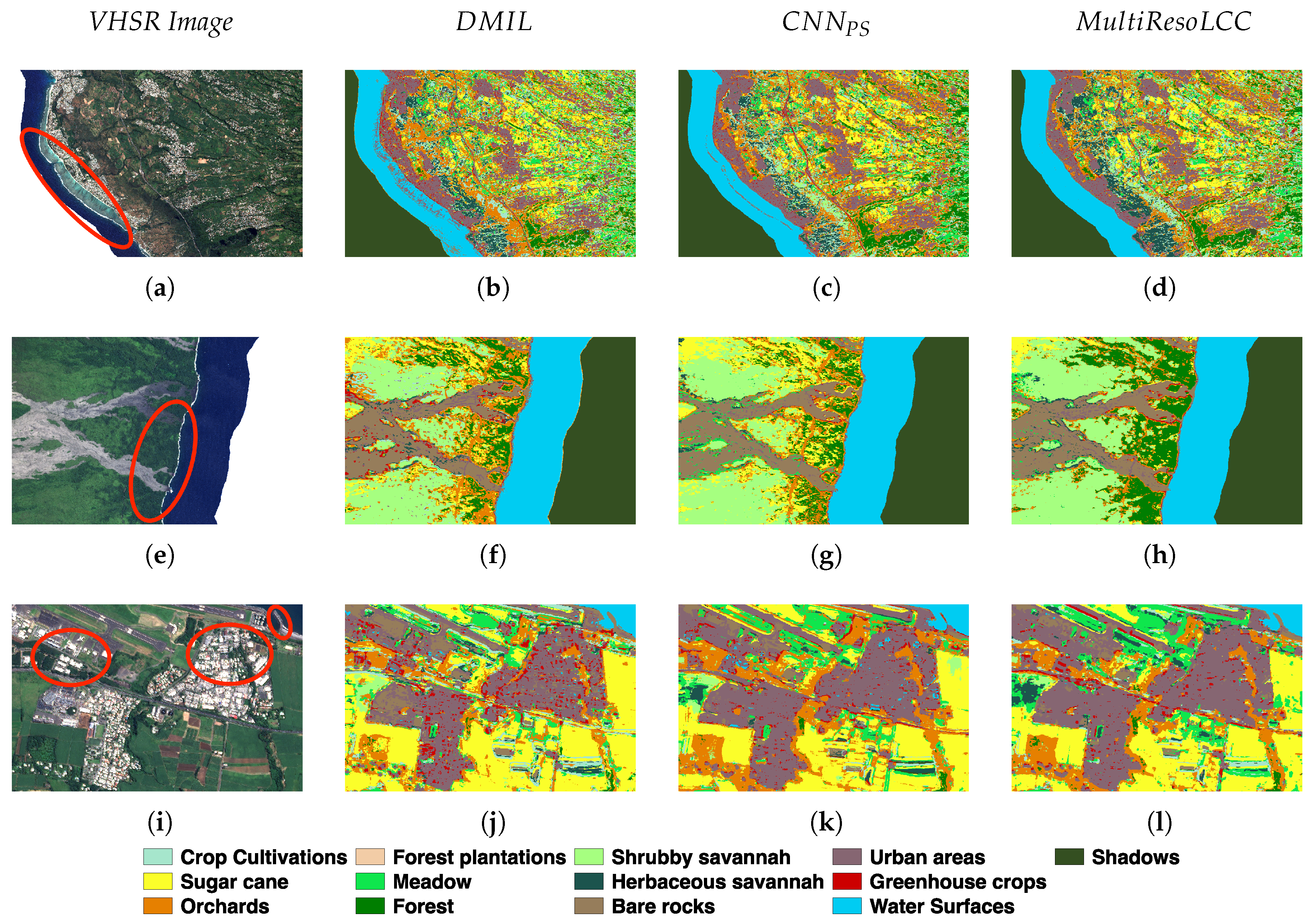
Concerning the Reunion Island dataset, the first example (Figure 8a–d) depicts a coastal area of the west coast of the island. Here, we highlight a zone that is characterized by an underwater coral reef. $DMIL$ and $CN{N}_{PS}$ have some troubles classifying this zone as water; more in detail they confused the true class and the Bare Rocks and Urban areas classes. Conversely, $MultiResoLCC$ does not have any issue with this point and it supplies a coherent water classification.

The second example (Figure 8e–h) represents a zone mainly characterized by forest. In this case, both $DMIL$ and $CN{N}_{PS}$ provide a noisy classification mixing Forest with Sugar Cane and Orchards. Conversely, when we analyze the land cover map produced by $MultiResoLCC$ (Figure 8h), we observe that the Forest classification is more spatially homogeneous and consistent with the reference data available in the corresponding VHSR image.

The third and last example related to the Reunion Island dataset is supplied in Figure 8i–l. This area is mainly characterized by an urban settlement surrounded by some agricultural plots. The three zones highlighted in this example involve zones belonging to Urban Areas and Bare rocks. Comparing the maps provided by $DMIL$ and $CN{N}_{PS}$ with respect to the one provided by $MultiResoLCC$, we can note that the formers made more confusion between Urban Areas/Bare rocks and Water Surfaces than the latter. $DMIL$ and $CN{N}_{PS}$ tend to overestimate the prediction of the Water Surfaces class. This phenomenon is more remarkable on the land cover map provided by $CN{N}_{PS}$ than the one supplied by $DMIL$. On the other hand, our approach has a more precise behavior on such classes and, as well as $DMIL$, it exploits the low-resolution information (multispectral bands) to regularize its spatial prediction.

Also on this study site $MultiResoLCC$ exhibits a satisfactory behavior considering the competing approaches. Similarly, to the analysis performed on the Gard study site, results are consistent with those reported in Table 8. Conversely to what was proposed in $DMIL$, the joint use of spatial and spectral information of the MS and PAN images at their native resolution, without any intermediate up-sampling step, provides useful regularization decreasing, at the same time, the confusion between land cover classes (i.e., Urban Areas vs Water Surfaces and Forest vs Orchards/Sugar Cane).

6. Conclusions

In this paper, a novel Deep Learning architecture to leverage PAN and MS imagery for land cover classification has been proposed. The approach, named $MultiResoLCC$, exploits multispectral and panchromatic information at their native resolutions. The architecture is composed of two branches, one for the PAN and one for the MS source. The final land cover classification is achieved by concatenating the features extracted by each branch. The framework is learned end-to-end from scratch.

The evaluation on two real-world study sites has shown that $MultiResoLCC$ achieves better quantitative and qualitative results than recent classification methods for optical VHSR images. In addition, the visual inspection of the land cover maps has underlined the effectiveness of our strategy and it advocates the use of both spatial and spectral information, at their native resolution, coming from PAN and MS imagery. Improving the quality of LULC maps will positively impacts the quality of the services built upon such thematic layer. For instance, the retrieval of zonal statistics on a geographical area as well as information retrieved querying a geospatial data warehouse to support environmental and urban planning.

As future work, we plan to extend the approach on other optical remote sensing images, for instance dealing with classification on Sentinel-2 satellite images where the spectral information is available at different spatial resolutions.

References

- Bégué, A.; Arvor, D.; Bellón, B.; Betbeder, J.; de Abelleyra, D.; Ferraz, R.P.D.; Lebourgeois, V.; Lelong, C.; Simões, M.; Verón, S.R. Remote Sensing and Cropping Practices: A Review. Remote Sens. 2018, 10, 99. [Google Scholar] [CrossRef]
- Georganos, S.; Grippa, T.; Vanhuysse, S.; Lennert, M.; Shimoni, M.; Wolff, E. Very High Resolution Object-Based Land Use-Land Cover Urban Classification Using Extreme Gradient Boosting. IEEE Geosci. Remote Sens. Lett. 2018, 15, 607–611. [Google Scholar] [CrossRef]
- Liu, X.; Jiao, L.; Zhao, J.; Zhao, J.; Zhang, D.; Liu, F.; Yang, S.; Tang, X. Deep Multiple Instance Learning-Based Spatial-Spectral Classification for PAN and MS Imagery. IEEE Trans. Geosci. Remote Sens. 2018, 56, 461–473. [Google Scholar] [CrossRef]
- Fasbender, D.; Radoux, J.; Bogaert, P. Bayesian Data Fusion for Adaptable Image Pansharpening. IEEE Trans. Geosci. Remote Sens. 2008, 46, 1847–1857. [Google Scholar] [CrossRef]
- Colditz, R.R.; Wehrmann, T.; Bachmann, M.; Steinnocher, K.; Schmidt, M.; Strunz, G.; Dech, S. Influence of image fusion approaches on classification accuracy: A case study. Int. J. Remote Sens. 2006, 27, 3311–3335. [Google Scholar] [CrossRef]
- Regniers, O.; Bombrun, L.; Lafon, V.; Germain, C. Supervised Classification of Very High Resolution Optical Images Using Wavelet-Based Textural Features. IEEE Trans. Geosci. Remote Sens. 2016, 54, 3722–3735. [Google Scholar] [CrossRef] [Green Version]
- Mura, M.D.; Benediktsson, J.A.; Waske, B.; Bruzzone, L. Morphological Attribute Profiles for the Analysis of Very High Resolution Images. IEEE Trans. Geosci. Remote Sens. 2010, 48, 3747–3762. [Google Scholar] [CrossRef]
- Wemmert, C.; Puissant, A.; Forestier, G.; Gançarski, P. Multiresolution Remote Sensing Image Clustering. IEEE Geosci. Remote Sens. Lett. 2009, 6, 533–537. [Google Scholar] [CrossRef]
- Storvik, G.; Fjørtoft, R.; Solberg, A.H.S. A bayesian approach to classification of multiresolution remote sensing data. IEEE Trans. Geosci. Remote Sens. 2005, 43, 539–547. [Google Scholar] [CrossRef]
- Zhang, L.; Du, B. Deep Learning for Remote Sensing Data: A Technical Tutorial on the State of the Art. IEEE Geosci. Remote Sens. Mag. 2016, 4, 22–40. [Google Scholar] [CrossRef]
- Liu, N.; Wan, L.; Zhang, Y.; Zhou, T.; Huo, H.; Fang, T. Exploiting Convolutional Neural Networks with Deeply Local Description for Remote Sensing Image Classification. IEEE Access 2018, 6, 11215–11228. [Google Scholar] [CrossRef]
- Guo, W.; Yang, W.; Zhang, H.; Hua, G. Geospatial Object Detection in High Resolution Satellite Images Based on Multi-Scale Convolutional Neural Network. Remote Sens. 2018, 10, 131. [Google Scholar] [CrossRef]
- Li, Y.; Zhang, Y.; Huang, X.; Zhu, H.; Ma, J. Large-Scale Remote Sensing Image Retrieval by Deep Hashing Neural Networks. IEEE Trans. Geosci. Remote Sens. 2018, 56, 950–965. [Google Scholar] [CrossRef]
- Tian, T.; Li, C.; Xu, J.; Ma, J. Urban Area Detection in Very High Resolution Remote Sensing Images Using Deep Convolutional Neural Networks. Sensors 2018, 18, 904. [Google Scholar] [CrossRef] [PubMed]
- Scott, G.J.; England, M.R.; Starms, W.A.; Marcum, R.A.; Davis, C.H. Training Deep Convolutional Neural Networks for Land-Cover Classification of High-Resolution Imagery. IEEE Geosci. Remote Sens. Lett. 2017, 14, 549–553. [Google Scholar] [CrossRef]
- Bengio, Y.; Courville, A.C.; Vincent, P. Representation Learning: A Review and New Perspectives. IEEE Trans. Pattern Anal. Mach. Intell. 2013, 35, 1798–1828. [Google Scholar] [CrossRef] [PubMed] [Green Version]
- Volpi, M.; Tuia, D. Dense Semantic Labeling of Subdecimeter Resolution Images with Convolutional Neural Networks. IEEE Trans. Geosci. Remote Sens. 2017, 55, 881–893. [Google Scholar] [CrossRef]
- Chaib, S.; Liu, H.; Gu, Y.; Yao, H. Deep Feature Fusion for VHR Remote Sensing Scene Classification. IEEE Trans. Geosci. Remote Sens. 2017, 55, 4775–4784. [Google Scholar] [CrossRef]
- Maggiori, E.; Tarabalka, Y.; Charpiat, G.; Alliez, P. Convolutional Neural Networks for Large-Scale Remote-Sensing Image Classification. IEEE Trans. Geosci. Remote Sens. 2017, 55, 645–657. [Google Scholar] [CrossRef]
- Bergado, J.R.; Persello, C.; Stein, A. Recurrent Multiresolution Convolutional Networks for VHR Image Classification. IEEE Trans. Geosci. Remote Sens. 2018, PP, 1–14. [Google Scholar] [CrossRef]
- Sun, W.; Wang, R. Fully Convolutional Networks for Semantic Segmentation of Very High Resolution Remotely Sensed Images Combined With DSM. IEEE Geosci. Remote Sens. Lett. 2018, 15, 474–478. [Google Scholar] [CrossRef]
- Audebert, N.; Saux, B.L.; Lefèvre, S. Semantic Segmentation of Earth Observation Data Using Multimodal and Multi-scale Deep Networks. In Proceedings of the Asian Conference on Computer Vision, Taipei, Taiwan, 20–24 November 2016; pp. 180–196. [Google Scholar]
- Noh, H.; Hong, S.; Han, B. Learning Deconvolution Network for Semantic Segmentation. In Proceedings of the IEEE International Conference on Computer Vision, Santiago, Chile, 7–13 December 2015; pp. 1520–1528. [Google Scholar]
- Xu, X.; Li, W.; Ran, Q.; Du, Q.; Gao, L.; Zhang, B. Multisource Remote Sensing Data Classification Based on Convolutional Neural Network. IEEE Trans. Geosci. Remote Sens. 2018, 56, 937–949. [Google Scholar] [CrossRef]
- Simonyan, K.; Zisserman, A. Very Deep Convolutional Networks for Large-Scale Image Recognition. arXiv, 2014; arXiv:1409.1556. [Google Scholar]
- Nair, V.; Hinton, G.E. Rectified Linear Units Improve Restricted Boltzmann Machines. In Proceedings of the 27th International Conference on Machine Learning, Haifa, Israel, 21–24 June 2010; pp. 807–814. [Google Scholar]
- Ioffe, S.; Szegedy, C. Batch Normalization: Accelerating Deep Network Training by Reducing Internal Covariate Shift. arXiv, 2015; arXiv:1502.03167. [Google Scholar]
- Ienco, D.; Gaetano, R.; Dupaquier, C.; Maurel, P. Land Cover Classification via Multitemporal Spatial Data by Deep Recurrent Neural Networks. IEEE Geosci. Remote Sens. Lett. 2017, 14, 1685–1689. [Google Scholar] [CrossRef] [Green Version]
- Dahl, G.E.; Sainath, T.N.; Hinton, G.E. Improving deep neural networks for LVCSR using rectified linear units and dropout. In Proceedings of the IEEE International Conference on Speech and Signal Processing, Vancouver, BC, Canada, 26–30 May 2013; pp. 8609–8613. [Google Scholar]
- Perez, L.; Wang, J. The Effectiveness of Data Augmentation in Image Classification using Deep Learning. arXiv, 2017; arXiv:1712.04621. [Google Scholar]
- Manuel, G.; Julien, M.; Victor, P.; Jordi, I.; Mickaël, S.; Rémi, C. Orfeo ToolBox: open source processing of remote sensing images. Open Geospat. Data Softw. Stand. 2017, 2, 15. [Google Scholar]
- Glorot, X.; Bengio, Y. Understanding the difficulty of training deep feedforward neural networks. In Proceedings of the Thirteenth International Conference on Artificial Intelligence and Statistics, Sardinia, Italy, 13–15 May 2010; pp. 249–256. [Google Scholar]
- Kingma, D.P.; Ba, J. Adam: A Method for Stochastic Optimization. arXiv, 2014; arXiv:1412.6980. [Google Scholar]
- Inglada, J.; Vincent, A.; Arias, M.; Tardy, B.; Morin, D.; Rodes, I. Operational High Resolution Land Cover Map Production at the Country Scale Using Satellite Image Time Series. Remote Sens. 2017, 9, 95. [Google Scholar] [CrossRef]
- Tan, P.N.; Steinbach, M.; Kumar, V. Introduction to Data Mining, 1st ed.; Addison-Wesley Longman Publishing Co., Inc.: Boston, MA, USA, 2005. [Google Scholar]
Figure 1.
General Overview of . The model is based on a two-branch CNN architecture to deal with panchromatic and multispectral information sources at their native resolution. The P-CNN branch is dedicated to panchromatic information while the -CNN branch deals with multispectral data. The extracted features are concatenated together and directly processed by a SoftMax classifier to provide the final land cover classification. Details about the P-CNN (respectively -CNN) branch are supplied in Figure 2 (respectively Figure 3).
Figure 2.
P-: Dedicated CNN Structure to manage Panchromatic information.
Figure 3.
MS-CNN: Dedicated CNN Structure to manage Multispectral information.
Figure 4.
SPOT6 panchromatic (a) and multispectral (b) images of the REUNION site.
Figure 5.
SPOT6 panchromatic (a) and multispectral (b) images of the GARD site.
Figure 6.
Confusion matrices of the deep learning approaches on the Reunion Island dataset ( (a), (b) and (c)) and on the Gard dataset ( (d), (e) and (f)). Values are normalized per class (row sum) in the interval [0,1].
Figure 7.
Visual inspection of Land Cover Map details produced on the Gard study site by , and on three different zones: (a–d) mixed area (tree crops, urban settlement and forest); (e–h) rural area and (i–l) wetland area.
Figure 8.
Visual inspection of Land Cover Map details produced on the Reunion Island study site by , and on three different zones: (a–d) coastal area; (e–h) forest area and (i–l) mixed area (urban settlement and agricultural plots).