A Discriminative Feature Learning Approach for Remote Sensing Image Retrieval


Research Institute of information Fusion, Naval Aviation University, Yantai 264001, China
*
Authors to whom correspondence should be addressed.
Remote Sens. 2019, 11(3), 281; https://doi.org/10.3390/rs11030281
Submission received: 30 December 2018
/
Revised: 23 January 2019
/
Accepted: 27 January 2019
/
Published: 1 February 2019
(This article belongs to the Special Issue Image Retrieval in Remote Sensing)
Abstract
:Effective feature representations play a decisive role in content-based remote sensing image retrieval (CBRSIR). Recently, learning-based features have been widely used in CBRSIR and they show powerful ability of feature representations. In addition, a significant effort has been made to improve learning-based features from the perspective of the network structure. However, these learning-based features are not sufficiently discriminative for CBRSIR. In this paper, we propose two effective schemes for generating discriminative features for CBRSIR. In the first scheme, the attention mechanism and a new attention module are introduced to the Convolutional Neural Networks (CNNs) structure, causing more attention towards salient features, and the suppression of other features. In the second scheme, a multi-task learning network structure is proposed, to force learning-based features to be more discriminative, with inter-class dispersion and intra-class compaction, through penalizing the distances between the feature representations and their corresponding class centers. Then, a new method for constructing more challenging datasets is first used for remote sensing image retrieval, to better validate our schemes. Extensive experiments on challenging datasets are conducted to evaluate the effectiveness of our two schemes, and the comparison of the results demonstrate that our proposed schemes, especially the fusion of the two schemes, can improve the baseline methods by a significant margin.

1. Introduction
As a result of the rapid development of remote sensing technology, the amount of remote sensing images with higher resolution has dramatically increased. How to effectively manage and analyze remote sensing images has been a hot issue to be solved urgently. Among them, content-based remote sensing image retrieval (CBRSIR) [1,2] is a key problem in the effective use of remote sensing big data. This includes two main components, feature extraction and similarity measure. CBRSIR automatically processes the representations of image features, and it measures the similarity between images. The performance of CBRSIR mainly depends on the representation power of feature embedding. Therefore, research on CBRSIR mainly focuses on feature extraction [3,4,5,6].
With regard to feature extraction, the existing methods can mainly be divided into methods that are based on handcrafted features, and methods based on learning-based features [7]. Handcrafted features are usually used to extract global features such as color, texture, shape, and local features based on SIFT [8] and SURF [9], which belong to low-level features. The Bag of Word model (BOW) [10,11,12], and the Vector of Locally Aggregated Descriptors (VLAD) [13] are proposed to encode local features, which further improve the feature representation power, they belong to the middle-level feature. Whether a global feature or a local feature, these handcrafted features are difficult for expressing image semantics precisely. That is, there is a “Semantic Gap” between low-level features and high-level semantics. With the progress of deep learning, especially the excellent performance of Convolutional Neural Networks (CNNs) in computer vision tasks such as classification [14,15,16], detection [17,18,19], and segmentation [20,21], CNNs are widely applied to image feature automatic extraction. The reason for why CNNs can achieve better performance than handcrafted features is that CNNs can extract high-level semantic features through a large number of convolutional layer stacking with non-linearity. Ge et al. [22] transfers the pre-trained CNNs trained on ImageNet to the remote sensing image data set and compares the features extracted by pre-trained CNNs with handcrafted features for CBRSIR, which leads to the conclusion that the CNNs features outperform the traditional features by a large margin.
However, it is difficult to achieve a satisfactory retrieval result only by pre-trained or fine-tuned CNNs, by facing the large-scale and high-resolution remote sensing image datasets. We think that this is mainly caused by the following two reasons. The first is insufficient representation power of feature embedding. In Figure 1, some examples of Aerial Image Data (AID) dataset [23] that are used for remote sensing image retrieval are shown. It can be inferred from Figure 1a,b that these two types of remote sensing images are characterized by color and texture features. From Figure 1c,d, we can see that they are characterized by the local shape of the aircraft and bridge instead of land and water occupying most areas of the image. Therefore, the features used for CBRSIR should be able to take into account both the global and local silent features of the image. However, pre-trained CNNs features may be difficult for meeting this requirement, due to the big difference between the ImageNet data set and the remote sensing image data set, and the difficulty of covering the images’ global and local silent features simultaneously with a convolutional layer or a fully connected layer. Some works [24,25,26] try to solve the above problems from the aspect of improving the data set, by introducing multi-labels and dense labeling remote sensing datasets for training. To a certain extent, this problem can be alleviated, while the disadvantage is also obvious that annotating on multi-labels is time-consuming and costly. The second reason is the inconsistency in the purpose between the training process and the retrieval process. Feature representation used in CBRSIR is the result of training for classification. The accuracy of classification can even reach 99% in the verification set and test set, while when it is used for image retrieval, the accuracy is far less than this. This is mainly due to the difference between classification and retrieval. In classification, softmax loss is usually used for training to encourage features to be separable, which leads the inter-class be disperse. However, in CBRSIR, the similarity is measured between the images by the Euclidean distance or the cosine distance, which requires feature representation not only to be separable but also discriminative. Discriminative features mean inter-class to disperse, and intra-class to be compact as much as possible.
In this paper, we propose two schemes as the response to the above problems. We first propose a new attention module for features extraction for CBRSIR, which can pay more attention to the silent features, and suppress the less useful ones. We then provide a center loss-based multi-task learning network structure to further boost the discriminative power of the features. The framework of our proposed method is shown in Figure 2.
The main contributions of this paper can be summarized as follows:
- To obtain salient and effective features, we propose a new attention module, which can be easily connected with the last convolutional layer of any pre-trained CNNs and can be applied along two dimensions: channel and spatial, attending to emphasize the meaningful features along these two axes.
- We propose a multi-task learning network structure, introducing center loss as a network branch in the training phase, to penalize the intra-class distances of features, and to improve the discriminative ability of the deep features.
- The two schemes that we proposed can be combined and integrated into the same training network to further improve performance.
The rest of this paper is organized as follows. Section 2 presents some published work that is related to features extraction for CBRSIR. Our proposed two schemes to generate discriminative feature representation are discussed in Section 3. Section 4 displays the experimental results and analysis. Section 5 includes a discussion, and Section 6 draws some conclusions.
2. Related Work
In the following section, we will present the related work on feature extraction, attention mechanism, and a loss function.
2.1. Learning-Based Feature Representation for CBRSIR
CNNs have been dominant in feature extraction, and have gradually replaced traditional methods in the field of computer vision. The achievement of CNNs is mainly due to the fact that deep network structures bring a large number of nonlinear functions, and weight parameters can be automatically learned from the training data. However, remote sensing image datasets cannot provide a large amount of data for CNNs training from scratch. CNNs pre-trained on massive datasets have been used to extract feature embedding, which has been proven to be effective and efficient, even when the training data set has a lot of difference with the remote sensing image. There are mainly two ways to exploit pre-trained CNNs, including regarding fully-connected layers or convolutional layers as the feature representation. Many works [3,22,27,28] have compared the performance of different feature representations extracted among the different networks and different layers. Ge, Jiang, Xu, Jiang and Ye [22] exploit representations from pre-trained CNNs, and feature combination and compression are adopted to improve the feature representation. The experimental results demonstrate that the pre-trained features and aggregated features are simple, and are able to improve retrieval performance. Zhou, Newsam, Li and Shao [28] propose to fine-tune the pre-trained CNNs on a remote sensing dataset, and they propose a novel CNN architecture based on a three-layer perceptron that has fewer parameters and that can learn low-dimensional features. The results show that the fine-tuned CNNs and the novel CNN are effective. Li et al. [29] proposes a novel approach based on deep hashing neural networks for large-scale RMIR. Deep feature learning networks and hashing learning networks are concluded in an end-to-end network. Zhou, Deng and Shao [26] propose a novel multi-label RSIR method using fully convolutional networks (FCN). A pixel-wise labeled dataset is used for training the FCN network. The segmentation maps of each remote sensing image are predicted and region convolutional features are extracted based on the segmentation maps. The experimental results show that the method achieves state-of-the-art performance. While these methods mainly focus on the depth and the width of network architecture, we pay more attention to “attention”.
2.2. Attention Mechanism
The attention mechanism is an important part of human perception. It focuses on a specific area of the image in “high resolution”, and it perceives the surrounding area of the image in “low resolution”, and then it continuously adjusts its focus point. Actually, the attention mechanism is involved in learning the weight distribution of different parts, which leads to different parts corresponding to different degrees of concentration. The benefits of this property have been proven in many tasks, ranging from machine translation and text summarization in sequence-based tasks to classification and segmentation in computer vision.
References [30,31,32] apply the weight-learned to the original image, and Wang et al. [33] apply the weight-learned to feature maps. In Hu et al. [34], the weight is applied to channel scales, to weight different channel features. Closer to our work, Woo et al. [35] exploits both channel and spatial-wise attention, and each of the attention mechanisms can acquire “what” and “where” to focus. All of these works are proposed for natural image processing, and they have shown their excellent performances in classification, detection and so on. There is no attention model for processing the remote sensing images.
2.3. The Loss Function
The effect of CNNs has been continuously improved, in addition to the improvement of the network structure, and the development of the loss function.
Softmax function is the most commonly used loss function to supervise the learning process for classification. Taking one image as an input, and outputting the image’s identification, this kind of model (softmax loss function) is called the identification model. Siamese networks are proposed in [36], which take a pair of images as input, and is called a verification model. This model can drive the distance to be closer for positive pairs, and further for negative pairs. After that, a model combining identification and verification is adopted in Reference [37,38], which makes the feature more discriminative. Besides, Schroff et al. [39] proposes triplet loss, and this has proven its effectiveness in many datasets. A model with triplet loss takes anchor, positive and negative three images as input, to minimize the distance between the anchor and the positive, and to maximize the distance between the anchor and the negative.
3. The Proposed Approach
3.1. Scheme 1—The Attention Module
Our attention module can be connected with the last convolutional layer of the pre-trained CNNs. As applied along two dimensions: channel and spatial, the attention module can be divided into the channel attention module and the spatial attention module. The attention module’s framework is shown in Figure 3.
3.1.1. The Channel Attention Module
Given the last convolutional layer F (H × W × C) of any CNNs as input, the channel attention module learns the channel attention map Mc (1 × 1 × C). As we all know, the last convolutional layer in CNNs contains the richest high-level semantic information, and the different channels are regarded as different features. For example, there are 2048 channels in the last convolutional layer of ResNet, and 512 channels in VGG. Not all of these 2048 or 512 features have equal contributions to feature representation. Thus, the vector Mc is learned, in order to weigh the importance of different channels. The progress of channel attention module is illustrated in Figure 4.
A typical average pooling method, global average pooling, is adopted, to squeeze the spatial dimension of the feature map to acquire the channel attention map Favg (1×1×C). Average pooling has been commonly used in some works [34,35], while Reference [35] suggest exploiting both the average pooling and the max pooling simultaneously, and this proves that their strategy is more effective than using each strategy independently. Different from References [34,35], the attention module in this paper is connected to the last convolutional layer of CNNs, not to each block. This is mainly because there is insufficient remote sensing data to enable the network to train from scratch. We apply average pooling in the attention module, which is connected to the pre-trained CNNs. The design choice of the different pooling methods and the effectiveness of our attention module is shown in Section 4.2.1. Then Favg connects with a multi-layer perceptron (MLP) with a hidden layer. The size of the hidden layer is set to C/r, where r is set to 2 in this study. After the MLP is the sigmoid function. Then, input F and the channel attention map Mc are multiplied by elementwise, to acquire the output channel-refined feature map. In conclusion, the channel attention module is computed as:
where W1∈RC/r×C and W0∈RC×C/r denote the weight of MLP, σ donates the sigmoid function, ⊗ denotes element-wise multiplication, and F′ is the final channel-refined feature map.
F′ = Mc ⊗ F = σ(MLP(AvgPool(F))) ⊗ F = σ(W1(W0(Favg))) ⊗ F
3.1.2. The Spatial Attention Module
The channel attention module is proposed for the difference between different channels, while the spatial attention module is aimed at a different spatial location. Human beings can easily capture informative features in an image by comparing the difference between the silent targets and the background. The differences between the silent targets and the background in the images reflect the differing importance of the different spatial locations in the feature maps.
As the complementary to channel attention module, the spatial attention module takes the output of the channel attention module as the input to yield the spatial attention map Ms, which focuses on weighing the importance of each spatial location in the feature map. Similar to the channel attention module, the average pooling is implemented first to acquire the map Fs (H × W × 1), but the difference is that the average pooling is applied along the channel axis. The choice of the different pooling ways is also verified in Section 4.2.1. The map Fs is regarded as an initial value of every pixel in the feature map. Then, a convolutional layer and a sigmoid function were used to generate the final weights of every location in the feature map. On the filter size used in the convolutional layer, the size adopted in Reference [35] is 7 × 7, but we have verified in Section 4.2.1 that a filter of size 3 × 3 can lead to a better performance than filters with other sizes in our attention module. At last, element-wise multiplication is applied to acquire the final refined output, F″. The detailed operation is computed as:
where σ donates the sigmoid function, and f 3×3 denotes the convolutional layer with a filter size of 3×3. The specific progress of spatial attention module can be seen in Figure 5.
F″ = Ms ⊗ F′ = σ(f 3×3(AvgPool (F′))) ⊗ F′ = σ(f 3×3(Fs)) ⊗ F′
3.2. Scheme 2—The Center Loss-Based Multi-Task Learning Network
In most of the CNNs, the softmax function is usually used as the loss function to supervise the training of the model. The softmax loss function is shown in Equation (3), and it can efficiently supervise the network trained for the classification task. The center loss function was proposed in Reference [40] to minimize the intra-class variations for face recognition task, as formulated in Equation (4).
where Cyi donates the class center of features, n is the number of classes, m donates the size of the mini-batch. During training, the update of the Cyi should consider all of the training sets in each iteration that is not impractical. In [40], the class center Cyi is updated, based on the mini-batch instead of all training sets. A scalar λ was used to control the learning rate of Cyi. The formulation of the improved loss function is given as Equation (5). The Stochastic Gradient Descent (SGD) can be used to optimize the parameters in the loss function, but the process of the back propagation is complicated, the specific algorithm can be found in Reference [40].
L = Ls + λ Lc
In this paper, a new network structure is proposed to leverage the center loss. The update of center Cyi is not decided by the average of the features of each class, which is complicated and time-consuming. We treat class center Cyi as the parameters to be learned. The Class centers are initialized to a matrix K of (n, k) where n is the number of classes and k donates the dimensions of the feature representation. The input of this branch is the label of the training image, which is the same as the output of the softmax branch. Through the input label, we can obtain the corresponding class center in the class centers matrix K. Thus, the center loss is calculated by minimizing the mean square error of the input image’s feature vector and center loss as formulated in Equation (6). From Reference [40], we can find that a proper value of λ can improve the performance of the features. Also, the hyper-parameter λ in Equation (5), which decides the intra-class variations, is set to 0.0001 in our experiment, which is verified in Section 4.2.2. As shown in Figure 6, the center loss is merged as a branch of the network, the class centers are learned and the distances between the features and their corresponding centers are minimized simultaneously. Our scheme is simpler, and the experiment is verified in Section 4.2.2.
4. Experiments and Analysis
4.1. Experimental Setup
The datasets used in our experiments are mainly AID [23] and ParttenNet [41], both of which contain a large number of remote sensing images.
The Aerial Image Data (AID) is composed of 30 categories of typical aerial scene images with a size of 600 × 600 pixels collected from Google Earth. The numbers of the images vary a lot with different classes, from 220 up to 420, for a total of 10,000 images. Examples from every category are shown in Figure 7a.
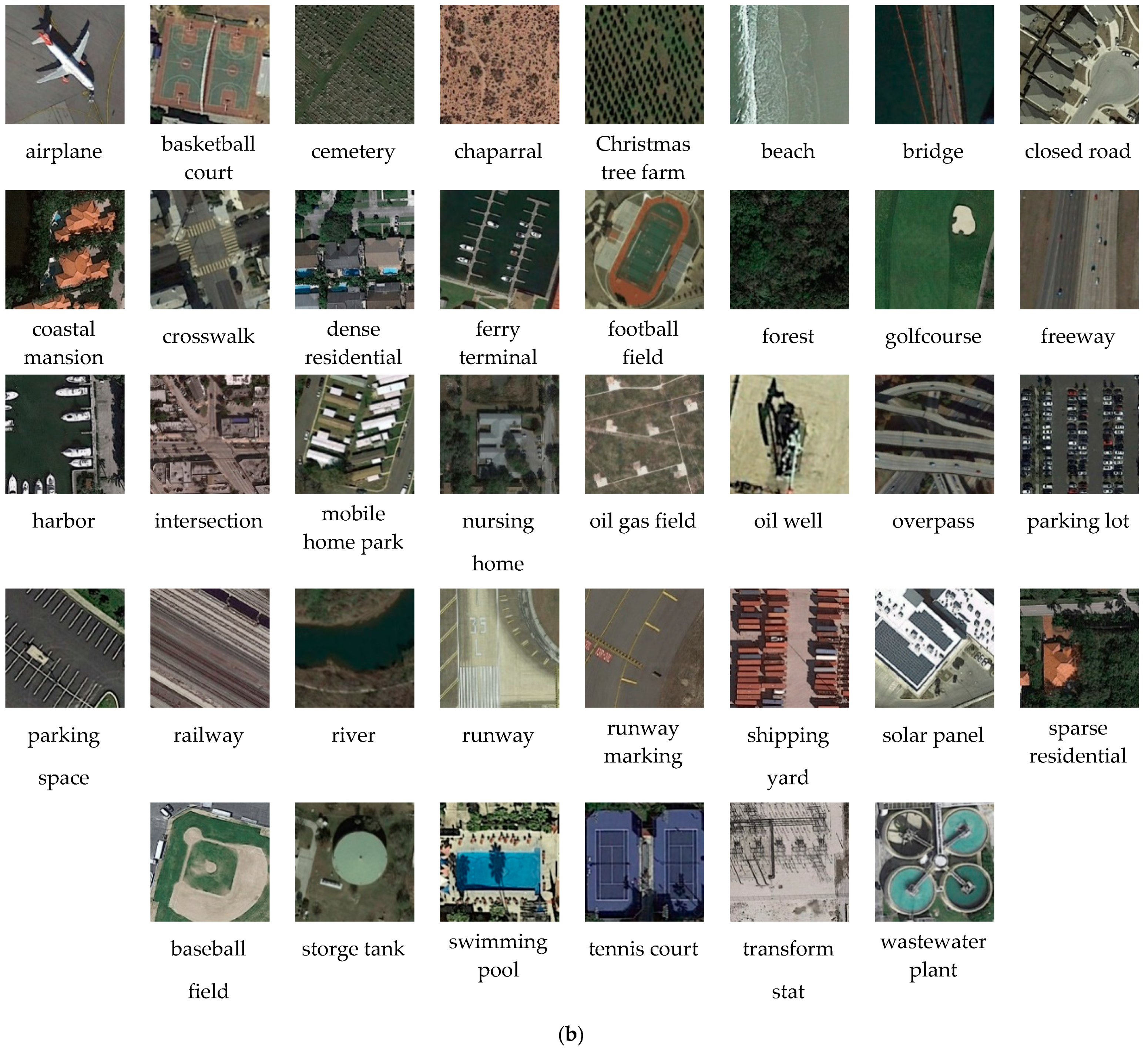
PatternNet comprises 38 categories of high-resolution remote sensing images with a size of 256 × 256 pixels selected from Google Earth. Each category contains 800 images, for a total of 30,400 images. Examples from every category are shown in Figure 7b.
Currently, datasets used for CBRSIR are mostly datasets for scene classification. However, there is an obvious difference between the classification and retrieval, and category labels are not available and are only used for accuracy evaluation in retrieval. However, some work conducts experiments on a data set, by dividing the data set into a training set and test set, and the category information has been utilized in the training process, which is contrary to the precondition of image retrieval. Different from this, in this paper, a challenging data set that is more in line with the preconditions of image retrieval is constructed to better verify the effectiveness of our method. The data set that is used for retrieval contains three subsets of the training set, probe set and test set, where the training set is different from the probe set and the test set. The label information in the training set is applied to fine-tune the pre-trained CNNs, but the labels are not available in the probe set and test set during the process of retrieval. Specifically, the data set AID is chosen as the training set to fine-tune the network pre-trained on ImageNet for its relatively huge amount of data and diverse data categories. The probe and test sets are selected from PatternNet. Twenty images are picked from each of the 38 categories in the PatternNet, a total of 760 images, forming the probe set. There are a total of 8162 images in the test set, of which 7600 are from PatternNet as ground truth, 200 in each category, and the remaining 562 images acting as interference are collected from other remote sensing image datasets and they are not related to the image of the PatternNet. These remote sensing image datasets includes RSSCN7 [42], UC Merced_landUse [43] and WHU-RS19 [44].
In the experiment, the Euclidean distance is used for the similarity measure. VGG16, VGG19 and ResNet50 are chosen as the baseline networks. The average normalized modified retrieval rank (ANMRR), the precision at k (P@k, k is the number of returned images), and the mean average precision (mAP) are used to assess the performance of CBRSIR. ANMRR and mAP can comprehensively evaluate the retrieval performance for it considering the order of all ground truths appearing in the retrieved images.
Besides, the class-level precision is adopted as another evaluation criteria. The precision of the i-th class can be expressed by n/ε, where n is the number of correct retrieval images of class i in the top ε retrieved images and ε is set to 20. Although the class-level precision cannot measure the performance of retrieval comprehensively like mAP and ANMRR for the reason that it is only the precision of the top 20 retrieved images, it can depict the precision of each class, and that it can reflect the differences among the different classes. It is worth noting that the lower values of ANMRR reflect better performance, while the larger the better, for mAP, P@k and class-level precision.
4.2. Results and Analysis
4.2.1. Design Choice and Effects of Scheme 1
In this section, the design process and the effectiveness of our attention module are shown. The design process of the module mainly consists of three parts. We first compare three ways of pooling strategies: max pooling, average pooling and the joint use of both two ways as in Reference [35], which are adopted in a channel attention module. The experimental results, with different pooling strategies, are shown in Table 1. On the one hand, we can observe that CNNs features, combined with the attention module, outperform the baselines, especially in VGG16 and VGG19. While the improvement in ResNet50 is not obvious, the main reason for this is that the performance of ResNet50 is relatively good, and that room for improvement is not as big as VGG. We observe that the attention module with any pooling methods is beneficial for improving the performance, compared with the baselines. On the other hand, the results imply the advantages of average pooling over the other two methods. The choice of average pooling can achieve better performance in both mAP and ANMRR, which improves the mAP from 0.5641 in VGG16, 0.5518 in VGG19 and 0.7080 in ResNet50 to 0.6 in VGG16, 0.5858 in VGG19, and 0.7187 in ResNet50. There are improvements of almost 4%, 2.5%, and 0.7% improvement for VGG16, VGG19, and ResNet50 in the value of ANMRR.
Second, we investigate the influences of three different filter sizes in the spatial attention module. The different spatial attention modules are placed after the previously designed channel attention module. Table 2 shows the experimental results. We can find that a smaller filter size leads to a better performance. This implies that the smaller receptive field can finely focus on each pixel, so that the importance of each pixel can be determined more accurately.
Thirdly, we compare our attention module to other popular attention modules: SE [34] and CBAM [35]. SE [34] and CBAM [35] are proposed for natural image processing, which inspired our attention module for remote sensing image processing. The experimental results are shown in Table 3. From mAP and ANMRR, it can be found that SE and CBAM cannot be adapted to the processing of remote sensing images. This is mainly because the SE and CBAM modify each block of the original network structure, and they need to be trained from scratch, while it is impossible to provide sufficient remote sensing image datasets to train the model from scratch. Our method adds the attention module to the end of the original network structure, and it can still take advantage of the pre-trained weights on ImageNet. The better mAP and ANMRR in Table 3 indicate our method is not only simple but effective. Besides, Figure 8 depicts that the baseline network connected with the average pooled attention module can achieve better performance for the majority of the classes. To better show the effect of our attention module, Gradient-weighted Class Activation Mapping (Grad-CAM) [45] is applied to visualize how the module is affecting the learning of the features. In Figure 9, we can find that the masks of the VGG16 combined with attention module cover the salient regions better than original VGG16, which indicates that the module-integrated networks can make full use of the information in salient regions and aggregate the features. Thus, these positive results show the superiority of our design choice and the effect of the attention module.
4.2.2. The Results of Scheme 2
In this part, we experimentally verify the effect of our scheme 2, by evaluating the performance of different CNNs trained under the supervision of different loss functions and making a comparison between our method and the baselines. A model combining identification loss and verification loss [37,38], and a model proposing triplet loss [39] are two popular and effective loss functions in natural image processing. The comparison between our method and the two methods is shown in Table 4. We observe that the models in References [37,38,39] are not as effective as dealing with natural images problems, such as face recognition and person re-identification. We believe that this is mainly because the remote sensing dataset is not as complex as the pedestrian dataset and face dataset. This means that more complex models [37,38,39] do not achieve better results based on relatively simple remote sensing datasets. Our method, a simpler loss function, is meaningful in improving the performance compared to References [37,38,39]. As depicted in Figure 10, we visualize the deep features of five classes obtained through the two training modes, to compare their differences intuitively, and Principal Component Analysis (PCA) is adopted to compress the 512-dimensional features obtained by VGG16 to two dimensions. Figure 10a,b exhibit the distribution of the softmax loss without center loss, and softmax loss with center loss. Figure 10c is the distribution of References [37,38], and (d) is Reference [39]. We can observe that the distribution of the same class in Figure 10b is more compact and that the features are relatively separable compared with Figure 10a,c,d. As a brief conclusion, the features trained under the softmax loss combined with the center loss, are more discriminative for its more dispersed inter-class and more compact intra-class.
Figure 11 shows the mAP of different models with different hyper-parameters λ. It is clear that the softmax loss (λ is 0) is not the best choice. The best performance is acquired when λ is set to 0.0001, and the performance decreases sharply as λ continues to increase. Figure 12 demonstrates the results of class-level precision, from which we can observe that ResNet50 outperforms the other two baselines, and the center loss can help CNNs to achieve better performance for the majority of the classes. The performance of our method and the original CNNs models is summarized in Table 5. There are improvements of almost 2%, 1%, and 0.7% for the baselines VGG16, VGG19, and ResNet50, respectively, in the values of mAP and ANMRR. We conclude that center loss is meaningful for boosting the discriminative power of deep features, comparing the ANMRR and mAP with the baseline networks.
4.2.3. The Effects of Combining Scheme 1 with Scheme 2
In this part, the effectiveness of combining our two schemes is empirically demonstrated. The attention module and the center loss are adopted simultaneously in the training phase, to acquire the discriminative deep features (as shown in Figure 2).
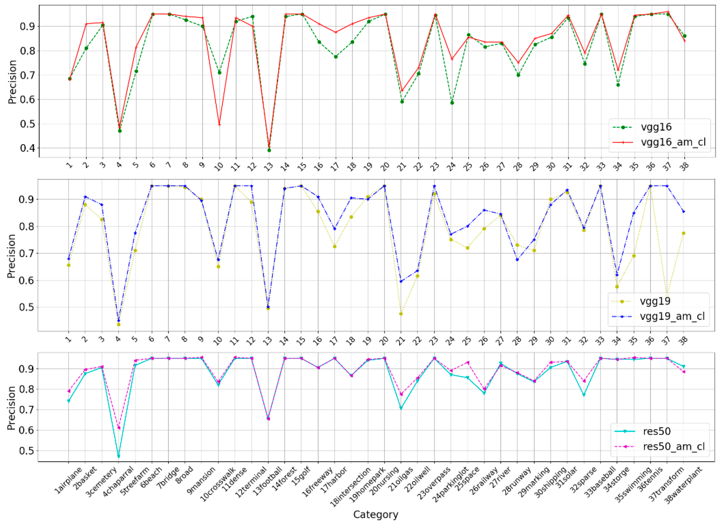
The results are shown in Table 6. We can see that the combined effect of the two schemes is generally better than any of the single schemes in terms of ANMRR and mAP. Our method increases the mAP of baseline VGG16 by nearly 5%, VGG19 by 4%, and ResNet50 by 1.2%. The improvement is similar on ANMRR. These results indicate that the feature representation generated under the combination of the two schemes is more discriminative and effective. The class-level precision is displayed in Figure 13.
4.2.4. Comparisons with the Baselines
In this part, the best result of our scheme is compared with a multi-label approach ReCNN+ [26] and several state-of-the-art approaches. We conduct the experiments under the same experimental conditions as ReCNN+ in [26]. The data set UC Merced_landUse is used, which contains 21 classes with 100 images per class, and 80% of the images are used for training, and the remaining 20% are used for evaluating the performance of the retrieval.
The results are shown in Table 7, from which we can see that our methods beat the multi-label approach ReCNN+ and other baselines with a large margin. The best performance in Reference [26] is ReCNN+, which achieves an ANMRR value of 0.264, the mAP value is 0.688. However, the CNNs-based features can achieve better performance, especially Resnet50. Our three methods have increased these two indicators by more than 10%, compared to Reference [26]. A 4%–9% improvement has been achieved, compared to the CNNs baseline. In addition, it can be found that the performance difference between our three methods is not large, and we think that this may be due to the smaller training and test sets. In conclusion, the CNNs-based features are effective, and they have good performance in CBRSIR, and our two schemes can further improve the performance of the CNNs.
5. Discussion
Through the above experiments and comparisons, the two schemes that we proposed can be proven to be effective. Based on the experimental results, we make some further discussion as follows:
- In the first scheme, the pre-trained CNNs connected with our simple attention module are regarded as the feature extractors. To give an extensive evaluation of our scheme, we conduct four comparative experiments: comparisons with fine-tuned VGG16, VGG19, and ResNet50, comparisons among different pooling methods, comparisons among different filter sizes, and comparisons with different attention modules. The results of experiment 1 in Table 1 show that our scheme is beneficial for improving the CNNs’ ability of feature representation. The results of experiments 2 and 3 in Table 1 and Table 2 show that the design choice of the attention module is appropriate and effective. The results of experiment 4 in Table 3 indicate that our attention module is more suitable for remote sensing images processing than SE [34] and CBAM [35], which are used for processing natural images. The attention module can further weight the features that are extracted by CNNs, to generate meaningful features that are more important, which is a possible explanation for the effects of our attention module.
- In the second scheme, a novel multi-task learning network structure that can further boost the discriminative power of the features is proposed based on center loss. By reducing the intra-class distance, the center loss that is adopted in our novel network further compensates for the lack of softmax loss. From the comparisons in Table 4 and the distributions in Figure 9, center loss, integrated with softmax loss, can achieve better performance than other loss functions [37,38,39], and more discriminative features, rather than just separable features, can be learned under the supervision of center loss. Better performance can be found in Table 5, compared with fine-tuned CNNs, which indicates that center loss is meaningful for boosting the discriminative power of deep features. Compared to the fine-tuned CNNs, a more compact intra-class distance is the key to the better performance of our scheme.
- The validity of the combination of scheme 1 and scheme 2 is verified in Section 4.2.3 and Section 4.2.4. The re-weighted feature maps caused by the attention module, and a more discriminative feature representation caused by center loss, are combined and compared with other schemes and baselines. The results in Table 6 and Table 7 show the remarkable performances of our combined schemes, which further validates the effectiveness of our two schemes and the feasibility of combining the two schemes.
- Learning-based features have attracted increasing interest not only in remote sensing image retrieval but also in the computer vision society. For example, most baselines in instance retrieval and person re-identification are learning-based features. Although the CNNs features are commonly adopted by remote sensing image retrieval and other retrieval tasks, the difference still exists. Specifically, person re-identification aims at retrieving a person of interest in other cameras, which is based on the person detection. The target of interest has been detected, there is almost no other interference information such as a background in the remote sensing image retrieval. Our scheme 1 is proposed for this point to focus on the salient target. Compared to instance retrieval, which is aiming to retrieve images containing the same object or architecture that may be captured under different views, remote sensing image retrieval belongs to class retrieval, which aims at retrieving images of the same class with the query, and this is why datasets used for CBRSIR are mostly datasets for remote sensing scene classification. Based on this, our scheme 2 is designed to penalize the intra-class distances of features. Our method is designed for the characteristics of remote sensing image retrieval and the particularity of the dataset.
6. Conclusions
In this paper, we proposed two schemes to acquire the discriminative features for remote sensing images retrieval. Our first scheme attention module, a simple module with small calculations, is applied to capture the silent local features and to suppress less useful ones. Through the execution of the two channel and spatial dimensions, our attention module can emphasize the important features along those two axes. Our second scheme center loss is adopted to improve the network structure of the original classification training. The advantage of center loss is to make the deep features of the inter-class dispersed and intra-class to be as compact as possible, which is more suitable for remote sensing images retrieval. To verify the validation of the approach, a more challenging data set is built, which consists of multiple published datasets for remote sensing images retrieval and scene classification. Finally, extensive experiments on the challenging data set and comparisons with baselines demonstrate the effectiveness and superiority of our two schemes, especially the combination of two schemes that can achieve the best performance.
Though our proposed feature learning approach can achieve better performance, there are still some shortcomings that we cannot neglect. As described in Section 3.1, our attention module can only be connected to the convolutional layer of CNNs. However, both the fully connected layer and the convolutional layer can be used as the feature representations. In Reference [27], the fully connected layer of some CNNs can obtain better retrieval performance than the convolutional layer under certain conditions. So, how to overcome the limitation for the use of the attention module is one of our future focuses. In addition, the attention module is proposed for remote sensing images retrieval, but it can also be used for other tasks, such as object detection and scene classification in remote sensing image processing.
Author Contributions
Conceptualization, W.X. and Y.L.; Formal analysis, Y.C.; Methodology, Y.L.; Software, Y.L. and X.Z.; Supervision, W.X. and Y.C.; Writing—original draft, Y.L.; Writing—review & editing, Y.C., X.Z. and X.G.
Funding
This research was funded by the [National Natural Science Foundation of China] grant number [61790550], [61790554] and [91538201].
Acknowledgments
The authors would like to thank the anonymous reviewers for their hard work.
Conflicts of Interest
The authors declare no conflict of interest.
References
- Du, P.; Chen, Y.; Hong, T.; Tao, F. Study on content-based remote sensing image retrieval. In Proceedings of the IEEE International Geoscience and Remote Sensing Symposium, Seoul, Korea, 29–29 July 2005; p. 4. [Google Scholar]
- Li, D. Content-based remote sensing image retrieval. Proc. SPIE Int. Soc. Opt. Eng. 2005, 6044, 60440Q. [Google Scholar]
- Napoletano, P. Visual descriptors for content-based retrieval of remote-sensing images. Int. J. Remote Sens. 2018, 39, 1343–1376. [Google Scholar] [CrossRef]
- Lu, L.Z.; Liu, R.Y.; Liu, N. Remote Sensing Image Retrieval Using Color and Texture Fused Features. J. Image Graph. 2004, 9, 328–333. [Google Scholar]
- Aptoula, E. Remote Sensing Image Retrieval with Global Morphological Texture Descriptors. IEEE Trans. Geosci. Remote Sens. 2014, 52, 3023–3034. [Google Scholar] [CrossRef]
- Zhu, X.X.; Tuia, D.; Mou, L.; Xia, G.S.; Zhang, L.; Xu, F.; Fraundorfer, F. Deep learning in remote sensing: A review. IEEE Geosci. Remote Sens. Mag. 2017, 5, 8–36. [Google Scholar] [CrossRef]
- Wan, J.; Wang, D.; Hoi, S.C.H.; Wu, P.; Zhu, J.; Zhang, Y.; Li, J. Deep Learning for Content-Based Image Retrieval:A Comprehensive Study. In Proceedings of the ACM International Conference on Multimedia, Orlando, FL, USA, 3–7 November 2014; pp. 157–166. [Google Scholar]
- Lowe, D.G. Object recognition from local scale-invariant features. In Proceedings of the Seventh IEEE International Conference on Computer Vision, Kerkyra, Greece, 20–27 September 1999; pp. 1150–1157. [Google Scholar]
- Bay, H.; Tuytelaars, T.; Van Gool, L. Surf: Speeded up robust features. In Proceedings of the European Conference on Computer Vision, Graz, Austria, 7–13 May 2006; pp. 404–417. [Google Scholar]
- Yang, J.; Liu, J.; Dai, Q. An improved Bag-of-Words framework for remote sensing image retrieval in large-scale image databases. Int. J. Digit. Earth 2015, 8, 273–292. [Google Scholar] [CrossRef]
- Sivic, J.; Zisserman, A. Video Google: A text retrieval approach to object matching in videos. In Proceedings of the Ninth IEEE International Conference on Computer Vision, Nice, France, 13–16 October 2003; p. 1470. [Google Scholar]
- Tang, X.; Zhang, X.; Liu, F.; Jiao, L. Unsupervised Deep Feature Learning for Remote Sensing Image Retrieval. Remote Sens. 2018, 10, 1243. [Google Scholar] [CrossRef]
- Jégou, H.; Douze, M.; Schmid, C.; Pérez, P. Aggregating local descriptors into a compact image representation. In Proceedings of the Computer Vision and Pattern Recognition (CVPR), San Francisco, CA, USA, 13–18 June 2010; pp. 3304–3311. [Google Scholar]
- Krizhevsky, A.; Sutskever, I.; Hinton, G.E. ImageNet classification with deep convolutional neural networks. In Proceedings of the International Conference on Neural Information Processing Systems, Long Beach, CA, USA, 4–9 December 2017; pp. 1097–1105. [Google Scholar]
- Szegedy, C.; Liu, W.; Jia, Y.; Sermanet, P.; Reed, S.; Anguelov, D.; Erhan, D.; Vanhoucke, V.; Rabinovich, A. Going deeper with convolutions. In Proceedings of the 2015 IEEE Conference on Computer Vision and Pattern Recognition (CVPR), Boston, MA, USA, 7–12 June 2015; pp. 1–9. [Google Scholar]
- He, K.; Zhang, X.; Ren, S.; Sun, J. Deep Residual Learning for Image Recognition. arXiv, 2015; 770–778arXiv:1512.03385. [Google Scholar]
- Lin, T.Y.; Dollar, P.; Girshick, R.; He, K.; Hariharan, B.; Belongie, S. Feature Pyramid Networks for Object Detection. In Proceedings of the IEEE Conference on Computer Vision and Pattern Recognition, Honolulu, HI, USA, 21–26 July 2017; pp. 936–944. [Google Scholar]
- Liu, W.; Anguelov, D.; Erhan, D.; Szegedy, C.; Reed, S.; Fu, C.Y.; Berg, A.C. SSD: Single Shot MultiBox Detector. In Proceedings of the European Conference on Computer Vision, Amsterdam, The Netherlands, 8–16 October 2016; pp. 21–37. [Google Scholar]
- Redmon, J.; Farhadi, A. YOLO9000: Better, Faster, Stronger. In Proceedings of the IEEE Conference on Computer Vision and Pattern Recognition, Honolulu, HI, USA, 21–26 July 2017; pp. 6517–6525. [Google Scholar]
- Long, J.; Shelhamer, E.; Darrell, T. Fully convolutional networks for semantic segmentation. In Proceedings of the IEEE Conference on Computer Vision and Pattern Recognition, Boston, MA, USA, 7–12 June 2015; pp. 3431–3440. [Google Scholar]
- Szegedy, C.; Ioffe, S.; Vanhoucke, V.; Alemi, A. Inception-v4, Inception-ResNet and the Impact of Residual Connections on Learning. arXiv, 2016; arXiv:1602.07261. [Google Scholar]
- Ge, Y.; Jiang, S.; Xu, Q.; Jiang, C.; Ye, F. Exploiting representations from pre-trained convolutional neural networks for high-resolution remote sensing image retrieval. Multimedia Tools Appl. 2017, 1–27. [Google Scholar] [CrossRef]
- Xia, G.S.; Hu, J.; Hu, F.; Shi, B.; Bai, X.; Zhong, Y.; Zhang, L.; Lu, X. AID: A Benchmark Data Set for Performance Evaluation of Aerial Scene Classification. IEEE Trans. Geosci. Remote Sens. 2016, PP, 1–17. [Google Scholar] [CrossRef]
- Shao, Z.; Yang, K.; Zhou, W. Performance Evaluation of Single-Label and Multi-Label Remote Sensing Image Retrieval Using a Dense Labeling Dataset. Remote Sens. 2018, 10, 964. [Google Scholar] [CrossRef]
- Chaudhuri, B.; Demir, B.; Chaudhuri, S.; Bruzzone, L. Multilabel Remote Sensing Image Retrieval Using a Semisupervised Graph-Theoretic Method. IEEE Trans. Geosci. Remote Sens. 2017, PP, 1–15. [Google Scholar] [CrossRef]
- Zhou, W.; Deng, X.; Shao, Z. Region Convolutional Features for Multi-Label Remote Sensing Image Retrieval. arXiv, 2018; arXiv:1807.08634. [Google Scholar]
- Xia, G.S.; Tong, X.Y.; Hu, F.; Zhong, Y.; Datcu, M.; Zhang, L. Exploiting Deep Features for Remote Sensing Image Retrieval: A Systematic Investigation. arXiv, 2017; arXiv:1707.07321. [Google Scholar]
- Zhou, W.; Newsam, S.; Li, C.; Shao, Z. Learning Low Dimensional Convolutional Neural Networks for High-Resolution Remote Sensing Image Retrieval. Remote Sens. 2016, 9, 489. [Google Scholar] [CrossRef]
- Li, Y.; Zhang, Y.; Huang, X.; Zhu, H.; Ma, J. Large-Scale Remote Sensing Image Retrieval by Deep Hashing Neural Networks. IEEE Trans. Geosci. Remote Sens. 2017, PP, 1–16. [Google Scholar] [CrossRef]
- Mnih, V.; Heess, N.; Graves, A.; Kavukcuoglu, K. Recurrent models of visual attention. Adv. Neural Inf. Process. Syst. 2014, 3, 2204–2212. [Google Scholar]
- Gregor, K.; Danihelka, I.; Graves, A.; Rezende, D.J.; Wierstra, D. DRAW: A recurrent neural network for image generation. Comput. Sci. 2015, arXiv:1502.04623, 1462–1471. [Google Scholar]
- Ba, J.; Mnih, V.; Kavukcuoglu, K. Multiple Object Recognition with Visual Attention. arXiv, 2014; arXiv:1412.7755. [Google Scholar]
- Wang, F.; Jiang, M.; Qian, C.; Yang, S.; Li, C.; Zhang, H.; Wang, X.; Tang, X. Residual Attention Network for Image Classification. In Proceedings of the Computer Vision and Pattern Recognition, Honolulu, HI, USA, 21–26 July 2017; pp. 6450–6458. [Google Scholar]
- Hu, J.; Shen, L.; Sun, G. Squeeze-and-Excitation Networks. arXiv, 2017; arXiv:1709.01507. [Google Scholar]
- Woo, S.; Park, J.; Lee, J.Y.; Kweon, I.S. CBAM: Convolutional Block Attention Module. arXiv, 2018; arXiv:1807.06521. [Google Scholar]
- Chopra, S.; Hadsell, R.; Lecun, Y. Learning a Similarity Metric Discriminatively, with Application to Face Verification. In Proceedings of the IEEE Computer Society Conference on Computer Vision and Pattern Recognition, CVPR 2005, San Diego, CA, USA, 20–25 June 2005; Volume 531, pp. 539–546. [Google Scholar]
- Wen, Y.; Li, Z.; Qiao, Y. Latent Factor Guided Convolutional Neural Networks for Age-Invariant Face Recognition. In Proceedings of the Computer Vision and Pattern Recognition, Las Vegas, NV, USA, 27–30 June 2016; pp. 4893–4901. [Google Scholar]
- Chen, Y.; Chen, Y.; Wang, X.; Tang, X. Deep learning face representation by joint identification-verification. In Proceedings of the International Conference on Neural Information Processing Systems, Montreal, QC, Canada, 8–13 December 2014; pp. 1988–1996. [Google Scholar]
- Schroff, F.; Kalenichenko, D.; Philbin, J. FaceNet: A unified embedding for face recognition and clustering. In Proceedings of the IEEE Conference on Computer Vision and Pattern Recognition, Boston, MA, USA, 7–12 June 2015; pp. 815–823. [Google Scholar]
- Wen, Y.; Zhang, K.; Li, Z.; Qiao, Y. A Discriminative Feature Learning Approach for Deep Face Recognition. In Proceedings of the Computer Vision—ECCV 2016: 14th European Conference, Amsterdam, The Netherlands, 11–14 October 2016; pp. 499–515. [Google Scholar]
- Zhou, W.; Newsam, S.; Li, C.; Shao, Z. PatternNet: A benchmark dataset for performance evaluation of remote sensing image retrieval. ISPRS J. Photogramm. Remote Sens. 2018, 145, 197–209. [Google Scholar] [CrossRef] [Green Version]
- Zou, Q.; Ni, L.; Zhang, T.; Wang, Q. Deep Learning Based Feature Selection for Remote Sensing Scene Classification. IEEE Geosci. Remote Sens. Lett. 2015, 12, 2321–2325. [Google Scholar] [CrossRef]
- Yang, Y.; Newsam, S. Bag-of-visual-words and spatial extensions for land-use classification. In Proceedings of the Sigspatial International Conference on Advances in Geographic Information Systems, San Jose, CA, USA, 2–5 November 2010; pp. 270–279. [Google Scholar]
- Xia, G.-S.; Yang, W.; Delon, J.; Gousseau, Y.; Sun, H.; Maître, H. Structural high-resolution satellite image indexing. In Proceedings of the ISPRS TC VII Symposium-100 Years ISPRS, Vienna, Austria, 5–7 July 2010; pp. 298–303. [Google Scholar]
- Selvaraju, R.R.; Cogswell, M.; Das, A.; Vedantam, R.; Parikh, D.; Batra, D. Grad-CAM: Visual Explanations from Deep Networks via Gradient-Based Localization. arXiv, 2016; arXiv:1610.02391. [Google Scholar]
Figure 1.
Some samples images from Aerial Image Data (AID). (a) desert, (b) forest, (c) airport, (d) bridge.
Figure 1.
Some samples images from Aerial Image Data (AID). (a) desert, (b) forest, (c) airport, (d) bridge.

Figure 2.
The framework of our proposed discriminative feature learning approach.

Figure 3.
Diagram of the attention module.

Figure 4.
Diagram of the channel attention module.

Figure 5.
Diagram of spatial attention module.

Figure 6.
Diagram of the Center Loss-based multi-task learning network structure.

Figure 7.
Samples images from the datasets AID and PatternNet, (a) examples from dataset AID, (b) examples from dataset PatternNet.
Figure 7.
Samples images from the datasets AID and PatternNet, (a) examples from dataset AID, (b) examples from dataset PatternNet.


Figure 8.
Class-level precisions of different baseline networks and the corresponding average pooled attention modules, where vgg16_am means the vgg16 combined with the average pooled attention module.
Figure 8.
Class-level precisions of different baseline networks and the corresponding average pooled attention modules, where vgg16_am means the vgg16 combined with the average pooled attention module.

Figure 9.
Grad-CAM (Gradient-weighted Class Activation Mapping) visualization results.

Figure 10.
The distribution of the learned features under the supervision of softmax loss and softmax combined center loss: (a) Softmax loss (b) Softmax loss + center loss (c) Reference [37], Reference [38]: identification loss+ verification loss, (d) Reference [39]: triplet loss.

Figure 11.
Models with different λ.

Figure 12.
Class-level precision of different baselines trained under different loss function. vgg16_cl means the vgg16 trained under the joint supervision of the softmax loss function and the center loss function.
Figure 12.
Class-level precision of different baselines trained under different loss function. vgg16_cl means the vgg16 trained under the joint supervision of the softmax loss function and the center loss function.

Figure 13.
Class-level precision of different baselines, and the scheme combining the attention module with center loss.
Figure 13.
Class-level precision of different baselines, and the scheme combining the attention module with center loss.


Table 1.
Comparisons of different attention modules by using different pooling methods. The best result for each baseline CNN (Convolutional Neural Network) is reported in bold.
Table 1.
Comparisons of different attention modules by using different pooling methods. The best result for each baseline CNN (Convolutional Neural Network) is reported in bold.
| Description | ANMRR | mAP | P@1 | P@5 | P@10 | P@20 | P@50 | P@100 |
|---|---|---|---|---|---|---|---|---|
| Vgg16(baseline) | 0.3691 | 0.5641 | 0.9368 | 0.8868 | 0.8342 | 0.7684 | 0.6684 | 0.5474 |
| Vgg16_Avgpool | 0.3283 | 0.6097 | 0.9474 | 0.9053 | 0.8789 | 0.8026 | 0.7474 | 0.5868 |
| Vgg16_Maxpool | 0.3376 | 0.5997 | 0.9447 | 0.8737 | 0.8921 | 0.7921 | 0.6921 | 0.5868 |
| Vgg16_Avg + Max | 0.3326 | 0.6011 | 0.9474 | 0.9316 | 0.8747 | 0.7947 | 0.7263 | 0.6026 |
| Vgg19(baseline) | 0.3717 | 0.5518 | 0.9263 | 0.8921 | 0.8447 | 0.7500 | 0.6500 | 0.5447 |
| Vgg19_Avgpool | 0.3473 | 0.5858 | 0.9605 | 0.9132 | 0.8920 | 0.7895 | 0.6868 | 0.5263 |
| Vgg19_Maxpool | 0.3683 | 0.5658 | 0.9237 | 0.8684 | 0.8211 | 0.7711 | 0.6474 | 0.5421 |
| Vgg19_Avg + Max | 0.3604 | 0.5727 | 0.9500 | 0.8921 | 0.8789 | 0.8053 | 0.6816 | 0.5316 |
| Res50(baseline) | 0.2335 | 0.7080 | 0.9668 | 0.9500 | 0.9263 | 0.8737 | 0.7789 | 0.6579 |
| Res50_Avgpool | 0.2267 | 0.7187 | 0.9816 | 0.9526 | 0.9237 | 0.8816 | 0.8211 | 0.6789 |
| Res50_Maxpool | 0.2413 | 0.7007 | 0.9842 | 0.9500 | 0.9368 | 0.8921 | 0.8158 | 0.6974 |
| Res50_Avg + Max | 0.2344 | 0.7086 | 0.9789 | 0.9605 | 0.9342 | 0.8789 | 0.7921 | 0.7132 |
Table 2.
Comparisons among different filter sizes. The best result is reported in bold.
| Description | ANMRR | mAP | P@1 | P@5 | P@10 | P@20 | P@50 | P@100 |
|---|---|---|---|---|---|---|---|---|
| Vgg16(baseline) | 0.3691 | 0.5641 | 0.9368 | 0.8868 | 0.8342 | 0.7684 | 0.6684 | 0.5474 |
| Vgg16_AM(3 × 3) | 0.3283 | 0.6097 | 0.9474 | 0.9053 | 0.8789 | 0.8026 | 0.7474 | 0.5868 |
| Vgg16_AM(5 × 5) | 0.3381 | 0.5959 | 0.9500 | 0.9000 | 0.8789 | 0.8000 | 0.6711 | 0.5447 |
| Vgg16_AM(7 × 7) | 0.3411 | 0.5946 | 0.9479 | 0.9116 | 0.8395 | 0.8000 | 0.6737 | 0.5816 |
Table 3.
Comparisons of different attention modules. The best result is reported in bold.
| Description | ANMRR | mAP |
|---|---|---|
| Vgg16(baseline) | 0.3691 | 0.5641 |
| Vgg16_AM | 0.3283 | 0.6097 |
| Vgg16_SE [34] | 0.4911 | 0.4296 |
| Vgg16_CBAM [35] | 0.4910 | 0.4316 |
Table 4.
Comparisons of the different loss functions. The best result is reported in bold.
| Description | ANMRR | mAP |
|---|---|---|
| Vgg16(baseline) | 0.3691 | 0.5641 |
| Vgg16_CL | 0.3410 | 0.5864 |
| Vgg16_[37,38] | 0.3603 | 0.5656 |
| Vgg16_[39] | 0.3622 | 0.5662 |
Table 5.
Comparisons of different CNNs (Convolutional Neural Networks) under different loss functions. CL means that the network is trained under the supervision of the softmax loss function and the center loss function. The best result for each baseline CNN is reported in bold.
Table 5.
Comparisons of different CNNs (Convolutional Neural Networks) under different loss functions. CL means that the network is trained under the supervision of the softmax loss function and the center loss function. The best result for each baseline CNN is reported in bold.
| Description | ANMRR | mAP | P@1 | P@5 | P@10 | P@20 | P@50 | P@100 |
|---|---|---|---|---|---|---|---|---|
| Vgg16(baseline) | 0.3691 | 0.5641 | 0.9368 | 0.8868 | 0.8342 | 0.7684 | 0.6684 | 0.5474 |
| Vgg16_CL | 0.3410 | 0.5864 | 0.9395 | 0.8921 | 0.8421 | 0.8105 | 0.6948 | 0.5421 |
| Vgg19(baseline) | 0.3717 | 0.5518 | 0.9263 | 0.8684 | 0.8447 | 0.7500 | 0.6500 | 0.5447 |
| Vgg19_CL | 0.3601 | 0.5604 | 0.9237 | 0.8921 | 0.8211 | 0.7711 | 0.6474 | 0.5421 |
| Res50(baseline) | 0.2335 | 0.7080 | 0.9668 | 0.9500 | 0.9263 | 0.8737 | 0.7789 | 0.6579 |
| Res50_CL | 0.2274 | 0.7153 | 0.9868 | 0.9658 | 0.9447 | 0.8816 | 0.8116 | 0.7079 |
Table 6.
Comparisons of three different schemes with the baseline networks. The best result for each baseline CNN (Convolutional Neural Network) is reported in bold.
Table 6.
Comparisons of three different schemes with the baseline networks. The best result for each baseline CNN (Convolutional Neural Network) is reported in bold.
| Description | ANMRR | mAP | P@1 | P@5 | P@10 | P@20 | P@50 | P@100 |
|---|---|---|---|---|---|---|---|---|
| Vgg16 | 0.3691 | 0.5641 | 0.9368 | 0.8868 | 0.8342 | 0.7684 | 0.6684 | 0.5474 |
| Vgg16_AM | 0.3283 | 0.6097 | 0.9474 | 0.9053 | 0.8789 | 0.8026 | 0.7474 | 0.5868 |
| Vgg16_CL | 0.3410 | 0.5864 | 0.9395 | 0.8921 | 0.8421 | 0.8105 | 0.6948 | 0.5421 |
| Vgg16_AM + CL | 0.3182 | 0.6111 | 0.9421 | 0.9132 | 0.9105 | 0.8132 | 0.7342 | 0.6000 |
| Vgg19 | 0.3717 | 0.5518 | 0.9263 | 0.8684 | 0.8447 | 0.7500 | 0.6500 | 0.5447 |
| Vgg19_AM | 0.3473 | 0.5858 | 0.9605 | 0.9132 | 0.8920 | 0.7895 | 0.6868 | 0.5263 |
| Vgg19_CL | 0.3601 | 0.5604 | 0.9237 | 0.8921 | 0.8211 | 0.7711 | 0.6474 | 0.5421 |
| Vgg19_AM + CL | 0.3437 | 0.5925 | 0.9500 | 0.9237 | 0.8816 | 0.8184 | 0.7000 | 0.5605 |
| Res50 | 0.2335 | 0.7080 | 0.9668 | 0.9500 | 0.9263 | 0.8737 | 0.7789 | 0.6579 |
| Res50_AM | 0.2267 | 0.7187 | 0.9816 | 0.9526 | 0.9237 | 0.8816 | 0.8211 | 0.6789 |
| Res50_CL | 0.2274 | 0.7153 | 0.9868 | 0.9658 | 0.9447 | 0.8816 | 0.8116 | 0.7079 |
| Res50_AM + CL | 0.2230 | 0.7203 | 0.9816 | 0.9605 | 0.9579 | 0.9105 | 0.8053 | 0.7026 |
Table 7.
Comparisons between our methods and the baselines. The best result is reported in bold.
| Description | ANMRR | mAP | P@5 | P@10 | P@20 | P@50 |
|---|---|---|---|---|---|---|
| Statistic | 0.820 | 0.156 | 0.273 | 0.182 | 0.131 | 0.098 |
| LBP | 0.740 | 0.217 | 0.480 | 0.327 | 0.218 | 0.121 |
| BOVW | 0.538 | 0.398 | 0.561 | 0.464 | 0.376 | 0.236 |
| ReCNN | 0.509 | 0.441 | 0.686 | 0.556 | 0.414 | 0.228 |
| ReCNN+ | 0.264 | 0.688 | 0.861 | 0.753 | 0.624 | 0.344 |
| Vgg16 | 0.196 | 0.728 | 0.871 | 0.841 | 0.816 | 0.614 |
| Vgg19 | 0.177 | 0.717 | 0.870 | 0.833 | 0.817 | 0.676 |
| Res50 | 0.092 | 0.817 | 0.916 | 0.909 | 0.883 | 0.781 |
| Vgg16_AM+CL | 0.081 | 0.813 | 0.895 | 0.876 | 0.848 | 0.783 |
| Vgg19_AM+CL | 0.114 | 0.797 | 0.893 | 0.881 | 0.803 | 0.771 |
| Res50_AM+CL | 0.089 | 0.840 | 0.919 | 0.914 | 0.921 | 0.845 |
© 2019 by the authors. Licensee MDPI, Basel, Switzerland. This article is an open access article distributed under the terms and conditions of the Creative Commons Attribution (CC BY) license (http://creativecommons.org/licenses/by/4.0/).
Share and Cite
MDPI and ACS Style
Xiong, W.; Lv, Y.; Cui, Y.; Zhang, X.; Gu, X. A Discriminative Feature Learning Approach for Remote Sensing Image Retrieval. Remote Sens. 2019, 11, 281. https://doi.org/10.3390/rs11030281
AMA Style
Xiong W, Lv Y, Cui Y, Zhang X, Gu X. A Discriminative Feature Learning Approach for Remote Sensing Image Retrieval. Remote Sensing. 2019; 11(3):281. https://doi.org/10.3390/rs11030281
Chicago/Turabian StyleXiong, Wei, Yafei Lv, Yaqi Cui, Xiaohan Zhang, and Xiangqi Gu. 2019. "A Discriminative Feature Learning Approach for Remote Sensing Image Retrieval" Remote Sensing 11, no. 3: 281. https://doi.org/10.3390/rs11030281
Note that from the first issue of 2016, this journal uses article numbers instead of page numbers. See further details here.