Impact of the Elevation Angle on CYGNSS GNSS-R Bistatic Reflectivity as a Function of Effective Surface Roughness over Land Surfaces

Abstract

The Earth’s surface bistatic reflectivity ${\mathsf{\Gamma }}_{\mathrm{L}\mathrm{H}\mathrm{C}\mathrm{P},\mathrm{C}\mathrm{y}\mathrm{G}\mathrm{N}\mathrm{S}\mathrm{S}}$ is experimentally characterized using the novel Global Navigation Satellite Systems Reflectometry (GNSS-R) L-band passive multistatic radar technique from the Cyclone Global Navigation Satellite Systems (CyGNSS) eight-microsatellite constellation. The focus of this study is to evaluate the influence of the GNSS satellites’ elevation angle ${\mathsf{\theta }}_{\mathrm{e}}$ on ${\mathsf{\Gamma }}_{\mathrm{L}\mathrm{H}\mathrm{C}\mathrm{P},\mathrm{C}\mathrm{y}\mathrm{G}\mathrm{N}\mathrm{S}\mathrm{S}}$, as a function of soil moisture content (SMC) and effective surface roughness parameter $\mathrm{h}$. As the average response, the change of the scattering regime at a global scale and considering also vegetated surfaces appears at ${\mathsf{\theta }}_{\mathrm{e}}$ ≈ 55°. This empirical observation is understood as a change on the dominant scattering term, from incoherent to coherent. Then, the correlation of ${\mathsf{\Gamma }}_{\mathrm{L}\mathrm{H}\mathrm{C}\mathrm{P},\mathrm{C}\mathrm{y}\mathrm{G}\mathrm{N}\mathrm{S}\mathrm{S}}$ and SMC is evaluated as a function of ${\mathsf{\theta }}_{\mathrm{e}}$ over specific sparsely vegetated target areas. The smoother the surface, the higher the angular variability of the Pearson correlation coefficients. Over croplands (e.g., Argentinian Pampas), an improved correlation coefficient is achieved over angular ranges where the coherent scattering regime becomes the dominant one. As such, this function depends on the surface roughness. The maximum correlation coefficients are found at different ${\mathsf{\theta }}_{\mathrm{e}}$ for increasing mean roughness levels: ${\mathrm{r}}_{\mathrm{P}\mathrm{a}\mathrm{m}\mathrm{p}\mathrm{a}\mathrm{s}}$ ≈ 0.78 at ${\mathsf{\theta }}_{\mathrm{e}}$ ≈ [60,70]°, ${\mathrm{r}}_{\mathrm{I}\mathrm{n}\mathrm{d}\mathrm{i}\mathrm{a}}$ ≈ 0.72 at ${\mathsf{\theta }}_{\mathrm{e}}$ ≈ [50,60]°, and ${\mathrm{r}}_{\mathrm{S}\mathrm{u}\mathrm{d}\mathrm{a}\mathrm{n}}$ ≈ 0.74 at ${\mathsf{\theta }}_{\mathrm{e}}$ ≈ [30,40]°. SMC retrieval algorithms based on GNSS-R multi-angular information could benefit from these findings, so as to improve the accuracy using single-polarized signals.

1. Introduction

Small satellites [1] are changing the paradigm in Earth remote sensing, taking advantage of innovative payloads (e.g., References [2,3,4]). As such, the operation of constellations of these instruments has the potential to observe Earth’s dynamic processes with a higher spatiotemporal sampling than traditional techniques. In particular, the so-called Global Navigation Satellite Systems Reflectometry (GNSS-R) [5] is a sort of L-band passive multi-static radar (as many transmitters as navigation satellites are in view) that provides a wide swath up to ≈1500 km [6,7,8]. GNSS-R spatiotemporal sampling properties could open new process insights on mesoscale studies [6], wind speed determination [9], soil moisture content (SMC) determination [10], and vegetation water content (VWC) monitoring. There are several on-going research activities dedicated to improve the spatiotemporal sampling properties of GNSS-R. The main parameters being evaluated are the number of in-orbit receivers, the use of beam-forming strategies, and the directivity of the down-looking antennas [6]. Several methods have been proposed to extract the geophysical information added to the GNSS signals in the scattering process over the Earth’s surface: (a) The Passive Reflectometry and Interferometry System (PARIS) or interferometric GNSS-R (iGNSS-R) that can provide higher precision in ocean altimetry measurements, but requires the use of high-gain antennas [6,8]; (b) the conventional GNSS-R (cGNSS-R) that requires only relatively low-gain antennas for scatterometry purposes [8]; and (c) the GPS interferometric reflectometry (GPS-IR) that can determine accurately SMC with potential application to the global GNSS network [11].

At present, several small satellites have been launched into space carrying a GNSS-R payload on-board, including the United Kingdom (U.K.)-Disaster Monitoring Constellation DMC-1 [2] in 2003, the U.K.-TechDemoSat TDS-1 [3] in 2014, and the Universitat Politècnica de Catalunya UPC’s ³Cat-2 in 2016 [4]. In 2012, the National Aeronautics and Space Administration (NASA) selected the CyGNSS mission led by the University of Michigan as a low cost and high science Earth Venture Space System [12]. CyGNSS, an eight-microsatellite constellation, was launched on December 15, 2016 into a low Earth orbit (LEO) with an inclination angle ≈ 35° [13]. The main objective of this mission is to estimate wind speed over tropical cyclones with an unprecedented spatiotemporal sampling of the ocean [14]. Each single CyGNSS microsatellite has two left-hand circular polarization (LHCP) down-looking antennas pointing to the Earth’s surface with an inclination angle of ≈28° on each side of the satellite ground track. The antennas’ gain is ≈ 14.7 dB (antenna boresight), and the main payload is the so-called Delay Doppler Mapping Instrument (DDMI), which generates delay Doppler maps (DDMs) [8] on-board using a coherent integration time ${\mathrm{T}}_{\mathrm{c}}$ = 1 ms, and applying an incoherent average over ${\mathrm{N}}_{\mathrm{i}\mathrm{n}\mathrm{c}}$ = 1000 samples.

The application of active (e.g., synthetic aperture radar (SAR)) and passive (e.g., microwave radiometry and GNSS-R) remote sensing techniques over land-surfaces is based on the variability of the dielectric properties due to changes in SMC and biomass. However, surface roughness significantly affects SMC retrieval, especially in the case of GNSS-R [15,16,17] and SAR [18,19,20]. In this work, the sensitivity of GNSS-R to SMC, and the effect of surface roughness are assessed as a function of the elevation angle ${\mathsf{\theta }}_{\mathrm{e}}$ (${\mathsf{\theta }}_{\mathrm{e}}$ = 90° at the normal direction to the Earth’s surface) [21]. This is a first step towards SMC retrieval using GNSS-R multi-angular information [22] because the ratio of the coherent-to-incoherent scattering components [23] depends on the surface roughness through ${\mathsf{\theta }}_{\mathrm{e}}$. The coherent scattering component is expected to be more sensitive to SMC because of its improved spatial resolution (limited by approximately the first Fresnel zone) and its scattering properties. This smaller footprint provides an improved estimation on the actual heterogeneity of the surface. As such, the sensitivity of GNSS-R to SMC should increase with higher ${\mathsf{\theta }}_{\mathrm{e}}$ because the size of the first Fresnel zone is lower at this geometry. On the other hand, the coherent scattering component is expected to increase with lower ${\mathsf{\theta }}_{\mathrm{e}}$ [24] because the effective surface roughness is lower at this angular range, in agreement with the Rayleigh criterion. This trade-off is assessed over different surface types using the CyGNSS Level 1 Science Data Record [12,25].

The remainder of the paper is organized as follows. Section 2 provides an overview of approaches for studies over land. Section 3 describes bistatic scattering properties relevant to GNSS-R. Section 4 describes the methodology. Section 5 presents global-scale results. Section 6 describes the impact of ${\mathsf{\theta }}_{\mathrm{e}}$ as a function of SMC and effective surface roughness parameter with a focus over land. Section 7 includes final discussions, and the conclusions are highlighted in Section 8.

2. GNSS-R Approaches for Studies over Land Surfaces

The use of different GNSS-R methods (iGNSS-R, cGNSS-R, and GPS-IR) for land-surface applications requires further research activities because the dielectric properties of this scattering medium make it more complex than the ocean surface. The first study (to the authors’ knowledge) on the potential use of GNSS-R for SMC estimation was published in 2000 [26]. Follow-on activities were proposed simultaneously to investigate the capabilities of GNSS-R for SMC determination using cGNSS-R [27,28,29] and GPS-IR [10,11,30,31]. The use of the polarimetric ratio (ratio of the reflected signals’ power at two different polarizations) on cGNSS-R data collected from two airborne experiments was further studied for biomass monitoring up to an above ground biomass (AGB) of ≈300 ton/ha, and for SMC determination because it can cancel out surface roughness effects [15,16]. A GNSS dual-polarization payload [4] was successfully tested over boreal forests during two experiments from a stratospheric balloon [32]. A comprehensive study over different land surface types was performed to further assess the use of dual-polarization information obtained during two airborne campaigns [33]. More recently, new important conclusions were also derived, such as: (a) the use of the GPS-IR for accurate SMC estimation was validated over multiple GPS test sites including vegetated surfaces [11,34]; (b) a sensitivity to SMC of ≈38 dB/(m³/m³) was measured over nearly bare-soil target areas using data from U.K. TDS-1 [35,36]; (c) a Pearson correlation coefficient of $\mathrm{r}$ ≈ −0.6 between one-year averaged polarimetric ratio from a GNSS-R experiment on-board the Soil Moisture Active Passive (SMAP) mission and SMC was measured over the complete Earth’s surface [16,37]; (d) ${\mathsf{\theta }}_{\mathrm{e}}$ should be considered for the application of the so-called Tau-Omega model in the GNSS-R case [35]; (e) the vegetation introduces short-term (volume scattering) and long-term (interference from large-size scatterers and canopy inhomogeneity) fluctuations on GNSS signals [38]; and (f) the unbiased root-mean-square difference between daily averaged CyGNSS-derived SMC and SMAP SMC is down to 0.045 cm³/cm³, after correcting for surface roughness effects [17].

3. Coherent and Incoherent Scattering in GNSS-R

The scattered electromagnetic field over land and ocean surfaces is composed of both a coherent and an incoherent contribution in different proportions depending on the dielectric and geometrical properties of the scattering medium, and the directions of incoming and outgoing electromagnetic waves. In the specular direction, the $\mathrm{p}$-polarized bistatic scattering coefficient ${\mathsf{\sigma }}_{\mathrm{p}}^0$ [39] can be assumed to be composed of an incoherent ${\mathsf{\sigma }}_{\mathrm{p},\mathrm{i}\mathrm{n}\mathrm{c}\mathrm{o}\mathrm{h}}^0$ and a coherent ${\mathsf{\sigma }}_{\mathrm{p},\mathrm{c}\mathrm{o}\mathrm{h}}^0$ term as it follows [40]:

$${\mathsf{\sigma }}_{\mathrm{p}}^0={\mathsf{\sigma }}_{\mathrm{p},\mathrm{i}\mathrm{n}\mathrm{c}\mathrm{o}\mathrm{h}}^0+{\mathsf{\sigma }}_{\mathrm{p},\mathrm{c}\mathrm{o}\mathrm{h}}^0$$

(1)

The estimation of ${\mathsf{\sigma }}_{\mathrm{p}}^0$ based on theoretical models requires several hypotheses, such as those regarding the dielectric permittivity of the lower media (land, ocean, …), and the distribution of the surface elevation slopes $\mathrm{Z}\mathrm{s}={\mathsf{\sigma }}_{\mathrm{R}\mathrm{M}\mathrm{S}}/\mathrm{L}$ [41]. The root mean square (RMS) of the surface height variation ${\mathsf{\sigma }}_{\mathrm{R}\mathrm{M}\mathrm{S}}$ and the surface correlation length $\mathrm{L}$ describe the statistical variation of the random component of the surface height relative to a reference surface, which determines the degree of surface roughness. The incoherent scattering term is dominant for moderate-to-strong surface roughness conditions, while the scattering is completely coherent for a flat surface.

The power of the incident and the scattered waves is related through the reflectivity of the scattering medium. The reflectivity is a physical property of the medium. It depends on its dielectric properties and the surface roughness. The reflectivity can be indirectly linked to, e.g., the SMC, and it is used as a fundamental observable in GNSS-R. GNSS-R is a sort of bistatic radar that allows for the collection of scattered GNSS signals along the specular direction. GNSS satellites transmit relatively low-power signals, and the scattering is strong only over an area around the nominal specular point (${\mathsf{\theta }}_{\mathrm{e},\mathrm{s}}={\mathsf{\theta }}_{\mathrm{e},\mathrm{i}}={\mathsf{\theta }}_{\mathrm{e}}$). GNSS signals are emitted with right-hand circular polarization (RHCP), although with a certain degree of ellipticity. After scattering over a surface, they become left-HCP (LHCP) for elevation angles ${\mathsf{\theta }}_{\mathrm{e}}$ higher than the Brewster angle, while they are mainly RHCP for lower ${\mathsf{\theta }}_{\mathrm{e}}$. Additionally, the scattering over biomass introduces a significant degree of depolarization. RHCP and LHCP reflected signals should be considered simultaneously in this case. The signal power collected by a GNSS reflectometer for LHCP (e.g., CyGNSS) is expressed by the so-called delay Doppler maps (DDMs), that can be derived under the bistatic radar equation as it follows [42]:

$$\langle {\left|{\mathrm{Y}}_{\mathrm{r}}(\mathsf{\tau },\mathrm{f})\right|}^2\rangle =\frac{{\mathrm{P}}_{\mathrm{T}}{\mathsf{\lambda }}^2}{{(4\mathsf{\pi })}^3}\iint \frac{{\mathrm{G}}_{\mathrm{T}}{\mathrm{G}}_{\mathrm{R}}{\left|\mathsf{\chi }(\mathsf{\tau },\mathrm{f})\right|}^2{\mathsf{\sigma }}_{\mathrm{L}\mathrm{H}\mathrm{C}\mathrm{P}}^0}{{\mathrm{R}}_{\mathrm{T}}^2{\mathrm{R}}_{\mathrm{R}}^2}{\mathrm{d}}^2\overline{\mathsf{\rho }}$$

(2)

where ${\mathrm{P}}_{\mathrm{T}}$ is the transmitted power, ${\mathrm{G}}_{\mathrm{T}}$ and ${\mathrm{G}}_{\mathrm{R}}$ are the transmitter and receiver antenna gains, $\mathsf{\chi }$ is the Woodward ambiguity function (WAF), ${\mathrm{R}}_{\mathrm{T}}$ and ${\mathrm{R}}_{\mathrm{R}}$ are, respectively, the ranges from the transmitter and the receiver to the specular point, ${\mathsf{\sigma }}_{\mathrm{L}\mathrm{H}\mathrm{C}\mathrm{P}}^0$ is the bistatic scattering coefficient at LHCP, and $\overline{\mathsf{\rho }}$ is the positioning vector of the scattering point.

GNSS-R LHCP-reflectivity ${\mathsf{\Gamma }}_{\mathrm{L}\mathrm{H}\mathrm{C}\mathrm{P}}$ includes both coherent ${\mathsf{\Gamma }}_{\mathrm{L}\mathrm{H}\mathrm{C}\mathrm{P},\mathrm{c}\mathrm{o}\mathrm{h}}$ and incoherent ${\mathsf{\Gamma }}_{\mathrm{L}\mathrm{H}\mathrm{C}\mathrm{P},\mathrm{i}\mathrm{n}\mathrm{c}\mathrm{o}\mathrm{h}}$ contributions in different proportions depending on satellites’ elevation angle, and the biomass, topography, and surface roughness. The coherently reflected power is related with ${\mathsf{\Gamma }}_{\mathrm{L}\mathrm{H}\mathrm{C}\mathrm{P},\mathrm{c}\mathrm{o}\mathrm{h}}$ as in [43]:

$$\langle {\left|{\mathrm{Y}}_{\mathrm{r},\mathrm{c}\mathrm{o}\mathrm{h}}(\mathsf{\tau },\mathrm{f})\right|}^2\rangle =\frac{{\mathrm{P}}_{\mathrm{T}}{\mathsf{\lambda }}^2{\mathrm{G}}_{\mathrm{T}}{\mathrm{G}}_{\mathrm{R}}{\left|\mathsf{\chi }(\mathsf{\tau },\mathrm{f})\right|}^2}{{(4\mathsf{\pi })}^2{({\mathrm{R}}_{\mathrm{T}}^{}+{\mathrm{R}}_{\mathrm{R}}^{})}^2}{\mathsf{\Gamma }}_{\mathrm{L}\mathrm{H}\mathrm{C}\mathrm{P},\mathrm{c}\mathrm{o}\mathrm{h}}$$

(3)

The surface roughness has a strong impact on the coherent reflectivity term ${\mathsf{\Gamma }}_{\mathrm{L}\mathrm{H}\mathrm{C}\mathrm{P},\mathrm{c}\mathrm{o}\mathrm{h}}$ that can be theoretically modelled as in [40]:

$${\mathsf{\Gamma }}_{\mathrm{L}\mathrm{H}\mathrm{C}\mathrm{P},\mathrm{c}\mathrm{o}\mathrm{h}}={\left|{\mathrm{R}}_{\mathrm{L}\mathrm{H}\mathrm{C}\mathrm{P}}({\mathsf{\theta }}_{\mathrm{e}})\right|}^2\exp (-{(2\mathrm{k}{\mathsf{\sigma }}_{\mathrm{R}\mathrm{M}\mathrm{S}}\mathrm{s}\mathrm{i}\mathrm{n}{\mathsf{\theta }}_{\mathrm{e}})}^2)$$

(4)

where ${\mathrm{R}}_{\mathrm{L}\mathrm{H}\mathrm{C}\mathrm{P}}$ is the polarized Fresnel reflection coefficient and $\mathrm{k}$ is the signal wavenumber. The impact of ${\mathsf{\theta }}_{\mathrm{e}}$ on ${\mathsf{\Gamma }}_{\mathrm{L}\mathrm{H}\mathrm{C}\mathrm{P},\mathrm{c}\mathrm{o}\mathrm{h}}$ is twofold; on one hand it affects the Fresnel reflection coefficient, and on the other hand, it effects the exponential decaying factor. For a completely flat surface, ${\mathsf{\sigma }}_{\mathrm{R}\mathrm{M}\mathrm{S}}$ is zero, and ${\mathsf{\Gamma }}_{\mathrm{L}\mathrm{H}\mathrm{C}\mathrm{P},\mathrm{c}\mathrm{o}\mathrm{h}}$ is equal to the square of the amplitude of the Fresnel reflection coefficient. ${\mathrm{R}}_{\mathrm{L}\mathrm{H}\mathrm{C}\mathrm{P}}$ is linked to the dielectric constant of the soil, and thus with SMC. For a given roughness and a fixed geometry, ${\mathsf{\Gamma }}_{\mathrm{L}\mathrm{H}\mathrm{C}\mathrm{P},\mathrm{c}\mathrm{o}\mathrm{h}}$ should increases with larger SMC. On the other hand, ${\mathrm{R}}_{\mathrm{L}\mathrm{H}\mathrm{C}\mathrm{P}}$ is nearly constant for ${\mathsf{\theta }}_{\mathrm{e}}$ > 40° and it decreases significantly for lower angles. However, the exponential factor increases significantly with lower ${\mathsf{\theta }}_{\mathrm{e}}$. As such, ${\mathsf{\Gamma }}_{\mathrm{L}\mathrm{H}\mathrm{C}\mathrm{P},\mathrm{c}\mathrm{o}\mathrm{h}}$ could be expected to be higher for grazing angles, even over areas with moderate roughness levels. Figure 1 shows the theoretical relationship (Equation (4)) between ${\mathsf{\Gamma }}_{\mathrm{L}\mathrm{H}\mathrm{C}\mathrm{P},\mathrm{c}\mathrm{o}\mathrm{h}}$ and ${\mathsf{\theta }}_{\mathrm{e}}$ for different levels of SMC. The Wang’s model [44] is used to relate the SMC with the dielectric constant of the soil, assuming a soil composition of 50% clay and 20% sand. It appears ${\mathsf{\Gamma }}_{\mathrm{L}\mathrm{H}\mathrm{C}\mathrm{P},\mathrm{c}\mathrm{o}\mathrm{h}}$ increases for lower ${\mathsf{\theta }}_{\mathrm{e}}$ and it decreases for higher ${\mathsf{\sigma }}_{\mathrm{R}\mathrm{M}\mathrm{S}}$. On the other hand, the influence of ${\mathsf{\theta }}_{\mathrm{e}}$ is higher as ${\mathsf{\sigma }}_{\mathrm{R}\mathrm{M}\mathrm{S}}$ increases. It could be expected that the coherently reflected power as collected from a spaceborne platform increases at grazing angles because it is roughly independent of the platform’s height (${\mathrm{R}}_{\mathrm{T}}^{}$ >> ${\mathrm{R}}_{\mathrm{R}}^{}$).

The expression of ${\mathsf{\Gamma }}_{\mathrm{L}\mathrm{H}\mathrm{C}\mathrm{P},\mathrm{i}\mathrm{n}\mathrm{c}\mathrm{o}\mathrm{h}}$ is quite complex and not compact. More detailed information on incoherent scattering over rough surfaces can be found in Reference [40]. The effects of biomass should be also considered for modeling the incoherent scattered field over vegetated areas. A comprehensive method can be found in Reference [29]. Finally, the impact of rough topography in ${\mathrm{Y}}_{\mathrm{r}}$ can be understood as a sort of impulse response in the delay and Doppler domains to be convolved with the WAF [45]. Rough topography reduces the spreading of the DDMs, while surface roughness increases the spreading with larger roughness because more specular reflection points contribute to the total scattered field. As such, Equation (4) is valid in regions without rough topography.

4. Data and Methods

In this work, the impact of the elevation angle ${\mathsf{\theta }}_{\mathrm{e}}$ on CyGNSS experimental reflectivity ${\mathsf{\Gamma }}_{\mathrm{L}\mathrm{H}\mathrm{C}\mathrm{P},\mathrm{C}\mathrm{y}\mathrm{G}\mathrm{N}\mathrm{S}\mathrm{S}}$ was empirically evaluated as a function of the effective surface roughness parameter $\mathrm{h}$ and SMC. CyGNSS Level 1 Science Data Record Version 2.0 [25] is used to estimate ${\mathsf{\Gamma }}_{\mathrm{L}\mathrm{H}\mathrm{C}\mathrm{P},\mathrm{C}\mathrm{y}\mathrm{G}\mathrm{N}\mathrm{S}\mathrm{S}}$ and SMAP Enhanced Level 3 product [46] is selected to provide $\mathrm{h}$ and SMC data. These observables are described here for an enhanced understanding of the experimental results.

CyGNSS experimental reflectivity ${\mathsf{\Gamma }}_{\mathrm{L}\mathrm{H}\mathrm{C}\mathrm{P},\mathrm{C}\mathrm{y}\mathrm{G}\mathrm{N}\mathrm{S}\mathrm{S}}$: The calibrated reflected and direct DDMs are used to estimate the power waveform peaks ${\mathrm{Y}}_{\mathrm{r},\mathrm{P}\mathrm{e}\mathrm{a}\mathrm{k},\mathrm{L}\mathrm{H}\mathrm{C}\mathrm{P}}$ and ${\mathrm{Y}}_{\mathrm{d},\mathrm{P}\mathrm{e}\mathrm{a}\mathrm{k},\mathrm{R}\mathrm{H}\mathrm{C}\mathrm{P}}$. They are computed using a coherent integration time of ${\mathrm{T}}_{\mathrm{c}}$ = 1 ms and 1000 samples to perform an incoherent averaging. The estimation of the CyGNSS reflectivity was obtained by applying the following algorithm:

$${\mathsf{\Gamma }}_{\mathrm{L}\mathrm{H}\mathrm{C}\mathrm{P},\mathrm{C}\mathrm{y}\mathrm{G}\mathrm{N}\mathrm{S}\mathrm{S}}=\langle {\left|{\mathrm{Y}}_{\mathrm{r},\mathrm{P}\mathrm{e}\mathrm{a}\mathrm{k},\mathrm{L}\mathrm{H}\mathrm{C}\mathrm{P}}\right|}^2\rangle /\langle {\left|{\mathrm{Y}}_{\mathrm{d},\mathrm{P}\mathrm{e}\mathrm{a}\mathrm{k},\mathrm{R}\mathrm{H}\mathrm{C}\mathrm{P}}\right|}^2\rangle$$

(5)

after compensating for the antennas’ gain patterns versus the gain at the corresponding boresight direction [down-looking gain ≈ 14.5 dB, ${\mathsf{\theta }}_{\mathrm{e}}$ = 62° and up-looking gain ≈ 4.7 dB, ${\mathsf{\theta }}_{\mathrm{e}}$ = 90°], and the difference of both gains at boresight. The compensation of the antennas’ gain was performed as a function of ${\mathsf{\theta }}_{\mathrm{e}}$, with a precision of four decimals. The half-power beamwidth (−3 dB) of each down-looking CyGNSS antenna was ≈30°, and the −6 dB field-of-view was ≈ 45°. On the other hand, each antenna pointed to the Earth’s surface with an inclination angle of 28° (antenna boresight). As such, GNSS signals reflected at lower ${\mathsf{\theta }}_{\mathrm{e}}$ ≈ [20,40]° could be accurately collected through the main lobe of each antenna.

Effective surface roughness parameter $\mathrm{h}$: It was empirically estimated based on the Moderate Resolution Imaging Spectroradiometer (MODIS) Geosphere-Biosphere Program (IGBP) land cover classes [47,48]. $\mathrm{h}$ is an estimation of the factor $4{\mathrm{k}}^2{\mathsf{\sigma }}_{\mathrm{R}\mathrm{M}\mathrm{S}}^2$ in the surface reflectivity term in Equation (4). As such, this parameterization provided an improved performance as compared to previous global constant values-based algorithms [49], because it incorporated the diversity of the land surface. $\mathrm{h}$ values for different land cover types are included in the SMAP Tau-Omega parameter look-up table, at a spatial scale of 9 km.

The use of physical roughness parameters, such as correlation length and RMS height, requires in situ characterization, which is time-consuming and it is not feasible at a global scale. Thus, the SMAP effective roughness parameter was selected for this study, although the ultimate accuracy of the MODIS IGBP land cover types used for the roughness parameter estimation in the SMAP algorithm needs to be further evaluated. This effective parameter accounts for the dependence of surface roughness with SMC, while physical parameters do not. A heterogeneous distribution of the water when the soil dries out more water at specific target areas creates variations in the actual roughness of the soil that is not considered by the physical parameters. Further research should also account for the effects of roughness dynamics. Over specific target areas it has been reported [50] that the actual soil roughness is slightly higher as compared to the estimation provided by physical roughness parameters. Future studies covering a large variety of areas could help to optimize the estimation of the effective roughness parameter at a global scale.

Soil Moisture Content (SMC): SMC was estimated using the single channel algorithm at V-Pol, when the optimal Earth’s surface conditions are identified. Then, the corrections for surface roughness [47,48], effective soil temperature, and vegetation water content (VWC) were applied.

5. Global Scale Reflectivity over Land and Ocean

The focus of this work is on the study of ${\mathsf{\Gamma }}_{\mathrm{L}\mathrm{H}\mathrm{C}\mathrm{P},\mathrm{C}\mathrm{y}\mathrm{G}\mathrm{N}\mathrm{S}\mathrm{S}}$ over land surfaces. As a first step, the evolution of ${\mathsf{\Gamma }}_{\mathrm{L}\mathrm{H}\mathrm{C}\mathrm{P},\mathrm{C}\mathrm{y}\mathrm{G}\mathrm{N}\mathrm{S}\mathrm{S}}$ is shown for three different ranges of ${\mathsf{\theta }}_{\mathrm{e}}$ over the complete coverage of the Earth’s surface provided by CyGNSS (Figure 2). Reflectivity data ${\mathsf{\Gamma }}_{\mathrm{L}\mathrm{H}\mathrm{C}\mathrm{P},\mathrm{C}\mathrm{y}\mathrm{G}\mathrm{N}\mathrm{S}\mathrm{S}}$ were averaged over one month (from 20 September to 20 October 2017) using a 0.1° × 0.1° latitude/longitude grid with a moving window of 0.2°. The spatial scale of the roughness parameter $\mathrm{h}$ and SMC is ≈9 km. The size of the CyGNSS’s footprint under the coherent scattering regime at ${\mathsf{\theta }}_{\mathrm{e}}$ ≈ 55° was ≈1 km across-track, and ≈7.6 km along-track. Thus, the gridding strategy enables the analysis using different sensors with different spatial resolution. This strategy also allows to determine the evolution of ${\mathsf{\Gamma }}_{\mathrm{L}\mathrm{H}\mathrm{C}\mathrm{P},\mathrm{C}\mathrm{y}\mathrm{G}\mathrm{N}\mathrm{S}\mathrm{S}}$ over a wider angular range and provides good sampling density at pixel level. This gridding was found to provide an improved correlation between CyGNSS reflectivity and the SMAP microwave brightness temperature [43]. Additionally, the application of this moving averaging filter minimized potential residual errors in the down-looking antenna gain pattern correction due to attitude determination and control system (ADCS) and in the estimation of the reflected ${\mathrm{Y}}_{\mathrm{r},\mathrm{P}\mathrm{e}\mathrm{a}\mathrm{k},\mathrm{L}\mathrm{H}\mathrm{C}\mathrm{P}}$ and direct ${\mathrm{Y}}_{\mathrm{d},\mathrm{P}\mathrm{e}\mathrm{a}\mathrm{k},\mathrm{R}\mathrm{H}\mathrm{C}\mathrm{P}}$ power waveforms peaks.

The averaged ${\mathsf{\Gamma }}_{\mathrm{L}\mathrm{H}\mathrm{C}\mathrm{P},\mathrm{C}\mathrm{y}\mathrm{G}\mathrm{N}\mathrm{S}\mathrm{S}}$ is displayed over land (Figure 2a,c,e) and ocean (Figure 2b,d,f) for different elevation angles in ranges of ${\mathsf{\theta }}_{\mathrm{e}}$ ≈ [70,90]° (Figure 2a,b), ${\mathsf{\theta }}_{\mathrm{e}}$ ≈ [45,65]° (Figure 2c,d), and ${\mathsf{\theta }}_{\mathrm{e}}$ ≈ [20,40]° (Figure 2e,f). Over land-surfaces (Figure 2a,c,e), there was a strong coherent scattering ${\mathsf{\sigma }}_{\mathrm{L}\mathrm{H}\mathrm{C}\mathrm{P},\mathrm{c}\mathrm{o}\mathrm{h}}^0$ and the width of the waveforms was much narrower than over the ocean. In this situation, the power fluctuations of ${\mathrm{Y}}_{\mathrm{r},\mathrm{P}\mathrm{e}\mathrm{a}\mathrm{k},\mathrm{L}\mathrm{H}\mathrm{C}\mathrm{P}}$ could be closely related to ${\mathsf{\sigma }}_{\mathrm{L}\mathrm{H}\mathrm{C}\mathrm{P},\mathrm{c}\mathrm{o}\mathrm{h}}^0$ at some areas. Additionally, the spatiotemporal variability of the permittivity over land surfaces was high. This explains the significant variability of ${\mathsf{\Gamma }}_{\mathrm{L}\mathrm{H}\mathrm{C}\mathrm{P},\mathrm{C}\mathrm{y}\mathrm{G}\mathrm{N}\mathrm{S}\mathrm{S}}$ (Figure 2a,c,e). Overall (

Table 1. Summary of the impact of the elevation angle ${\mathsf{\theta }}_{\mathrm{e}}$ on ${\mathsf{\Gamma }}_{\mathrm{L}\mathrm{H}\mathrm{C}\mathrm{P},\mathrm{C}\mathrm{y}\mathrm{G}\mathrm{N}\mathrm{S}\mathrm{S}}$ over land and ocean.

[dB]	${\mathsf{\Gamma }}^{\mathbf{20}\mathbf{°}\mathbf{<}{\mathsf{\theta }}_{\mathbf{e}}\mathbf{<}\mathbf{40}\mathbf{°}}$	${\mathsf{\Gamma }}^{\mathbf{45}\mathbf{°}\mathbf{<}{\mathsf{\theta }}_{\mathbf{e}}\mathbf{<}\mathbf{65}\mathbf{°}}$	${\mathsf{\Gamma }}^{\mathbf{70}\mathbf{°}\mathbf{<}{\mathsf{\theta }}_{\mathbf{e}}\mathbf{<}\mathbf{90}\mathbf{°}}$
Land	−12.1	−17.7	−15.8
Ocean	−14.1	−20.3	−19.4

), it appears ${\mathsf{\Gamma }}_{\mathrm{L}\mathrm{H}\mathrm{C}\mathrm{P},\mathrm{C}\mathrm{y}\mathrm{G}\mathrm{N}\mathrm{S}\mathrm{S}}$ increased from ${\mathsf{\theta }}_{\mathrm{e}}$ ≈ [70,90]° to ${\mathsf{\theta }}_{\mathrm{e}}$ ≈ [20,40]°: ${\mathsf{\Gamma }}_{\mathrm{L}\mathrm{a}\mathrm{n}\mathrm{d}}^{{}_{70°<{\mathsf{\theta }}_{\mathrm{e}}<90°}}$ ≈ −15.8 dB, ${\mathsf{\Gamma }}_{\mathrm{L}\mathrm{a}\mathrm{n}\mathrm{d}}^{{}_{20°<{\mathsf{\theta }}_{\mathrm{e}}<40°}}$ ≈ −12.1 dB, ${\mathsf{\Gamma }}_{\mathrm{O}\mathrm{c}\mathrm{e}\mathrm{a}\mathrm{n}}^{{}_{70°<{\mathsf{\theta }}_{\mathrm{e}}<90°}}$ ≈ −19.4 dB, and ${\mathsf{\Gamma }}_{\mathrm{O}\mathrm{c}\mathrm{e}\mathrm{a}\mathrm{n}}^{{}_{20°<{\mathsf{\theta }}_{\mathrm{e}}<40°}}$ ≈ −14.1 dB. These experimental results can be explained because of the strong impact of ${\mathsf{\theta }}_{\mathrm{e}}$ on ${\mathsf{\Gamma }}_{\mathrm{L}\mathrm{H}\mathrm{C}\mathrm{P},\mathrm{c}\mathrm{o}\mathrm{h}}$. The coherent scattering was very high for grazing angle, because the effective surface roughness was low [51]. As such, the reflectivity was much higher at ${\mathsf{\theta }}_{\mathrm{e}}$ ≈ [20,40]° than at ${\mathsf{\theta }}_{\mathrm{e}}$ ≈ [70,90]°. On the other hand, ${\mathsf{\Gamma }}_{\mathrm{L}\mathrm{H}\mathrm{C}\mathrm{P},\mathrm{C}\mathrm{y}\mathrm{G}\mathrm{N}\mathrm{S}\mathrm{S}}$ decreased from ${\mathsf{\theta }}_{\mathrm{e}}$ ≈ [70,90]° to ${\mathsf{\theta }}_{\mathrm{e}}$ ≈ [45,65]° because the incoherent scattering is dominant over the coherent one in this angular range: ${\mathsf{\Gamma }}_{\mathrm{L}\mathrm{a}\mathrm{n}\mathrm{d}}^{{}_{45°<{\mathsf{\theta }}_{\mathrm{e}}<65°}}$ ≈ −17.7 dB and ${\mathsf{\Gamma }}_{\mathrm{O}\mathrm{c}\mathrm{e}\mathrm{a}\mathrm{n}}^{{}_{45°<{\mathsf{\theta }}_{\mathrm{e}}<65°}}$ ≈ −20.3 dB. The incoherent or diffuse scattering was lower with decreasing ${\mathsf{\theta }}_{\mathrm{e}}$ because this term is generated by the effective surface roughness, which in turn decreased for lower ${\mathsf{\theta }}_{\mathrm{e}}$. This point explains the evolution of ${\mathsf{\Gamma }}_{\mathrm{L}\mathrm{H}\mathrm{C}\mathrm{P},\mathrm{C}\mathrm{y}\mathrm{G}\mathrm{N}\mathrm{S}\mathrm{S}}$ along this angular range. Additionally it is worth noting that the Brewster angle could potentially appear in the range ${\mathsf{\theta }}_{\mathrm{e}}$ ≈ [20,40]°. In this situation, the power of the RHCP-reflected GNSS signals would dominate that of LHCP-reflected ones. ${\mathsf{\Gamma }}_{\mathrm{L}\mathrm{H}\mathrm{C}\mathrm{P},\mathrm{C}\mathrm{y}\mathrm{G}\mathrm{N}\mathrm{S}\mathrm{S}}$ was higher at ${\mathsf{\theta }}_{\mathrm{e}}$ ≈ [20,40]° than at ${\mathsf{\theta }}_{\mathrm{e}}$ ≈ [70,90]° (Figure 2), although ${\mathsf{\Gamma }}_{\mathrm{L}\mathrm{H}\mathrm{C}\mathrm{P},\mathrm{C}\mathrm{y}\mathrm{G}\mathrm{N}\mathrm{S}\mathrm{S}}$ would decrease for lower ${\mathsf{\theta }}_{\mathrm{e}}$ < 20° especially over vegetated surfaces.

GNSS signals were attenuated and depolarized by the vegetation cover. This attenuation can be modeled as ${\mathrm{L}}^{\mathrm{c}\mathrm{a}\mathrm{n}\mathrm{o}\mathrm{p}\mathrm{y}}={\mathrm{e}}^{{\mathsf{\tau }}^{\mathrm{c}\mathrm{a}\mathrm{n}\mathrm{o}\mathrm{p}\mathrm{y}}/\sin {\mathsf{\theta }}_{\mathrm{e}}}$, where ${\mathsf{\tau }}^{\mathrm{c}\mathrm{a}\mathrm{n}\mathrm{o}\mathrm{p}\mathrm{y}}$ is the vegetation optical depth (VOD) of the vegetation layer. The attenuation is due to scattering and absorption when GNSS signals propagates through the vegetation, and thus it increases for lower ${\mathsf{\theta }}_{\mathrm{e}}$. The vertical stalks scatter more the vertically polarized waves than the horizontal ones. This geometrical effect contributes to the depolarization of the GNSS signals. Here, two land-cover types are selected to show different scenarios:

a)

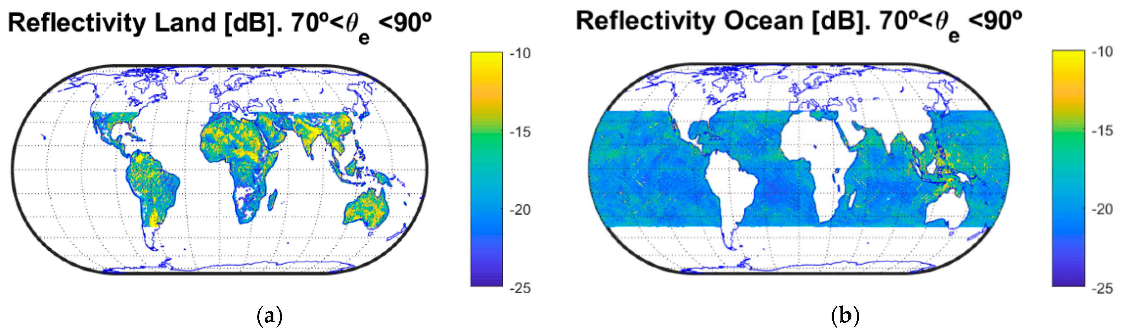
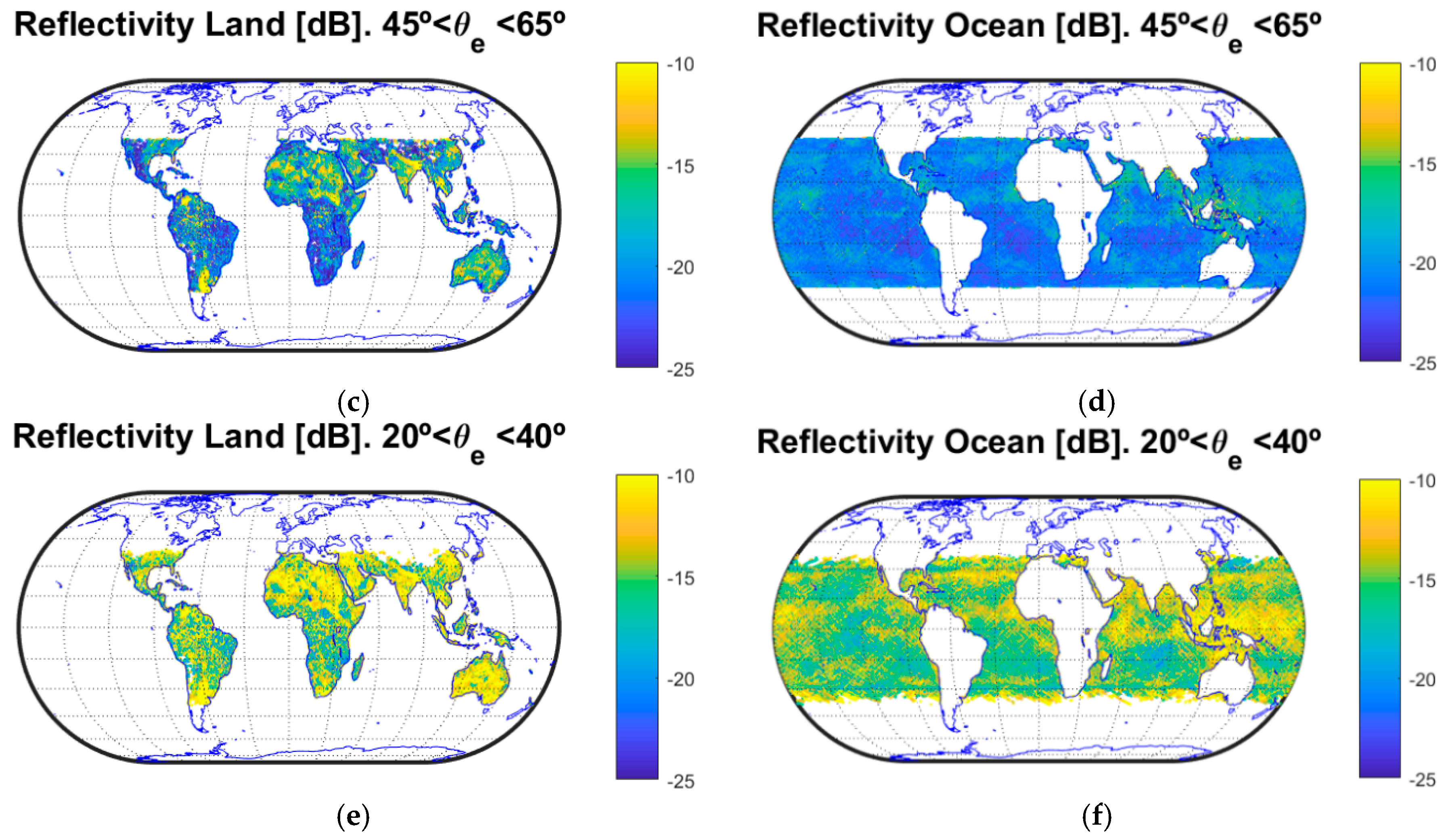
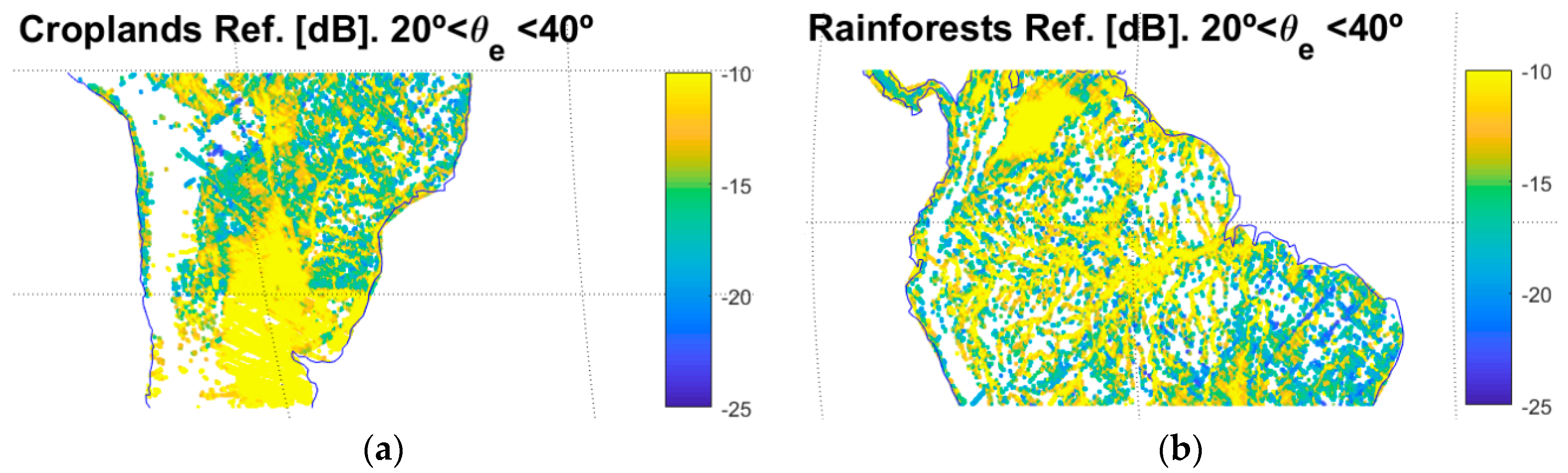
Croplands (target area at Lat = [−37,30]°, Lon = [−65,−60]°): This target area was sparsely vegetated and the surface roughness levels were relatively homogeneous due to agricultural activities. The mean ${\mathsf{\Gamma }}_{\mathrm{L}\mathrm{H}\mathrm{C}\mathrm{P},\mathrm{C}\mathrm{y}\mathrm{G}\mathrm{N}\mathrm{S}\mathrm{S}}$ increased by ≈4.2 dB from ${\mathsf{\theta }}_{\mathrm{e}}$ ≈ [70,90]° to ${\mathsf{\theta }}_{\mathrm{e}}$ ≈ [20,40]° as an indication of a higher signal coherence for lower ${\mathsf{\theta }}_{\mathrm{e}}$ (Figure 3a). This ${\mathsf{\Gamma }}_{\mathrm{L}\mathrm{H}\mathrm{C}\mathrm{P},\mathrm{C}\mathrm{y}\mathrm{G}\mathrm{N}\mathrm{S}\mathrm{S}}$ gradient could be only attributed to angular changes on the surface scattering mechanisms because the signal attenuation through the vegetation could be assumed to be negligible in this target area.

b)

Amazonian rainforests (target area at Lat = [−8,1]°, Lon = [−75, −65]°): This target area was characterized by wet biomass with high AGB ≈ 350 tons/ha that strongly attenuated GNSS signals, so that the remaining reflected power could be interpreted as a noise power floor in ${\mathrm{Y}}_{\mathrm{r},\mathrm{P}\mathrm{e}\mathrm{a}\mathrm{k},\mathrm{L}\mathrm{H}\mathrm{C}\mathrm{P}}$ (areas in “white” in Figure 3b correspond to SNR lower than 3 dB). However, the increment due to the coherent scattering ${\mathsf{\sigma }}_{\mathrm{L}\mathrm{H}\mathrm{C}\mathrm{P},\mathrm{c}\mathrm{o}\mathrm{h}}^0$ over soil and inland water bodies compensated this attenuation, and as a consequence, the mean ${\mathsf{\Gamma }}_{\mathrm{L}\mathrm{H}\mathrm{C}\mathrm{P},\mathrm{C}\mathrm{y}\mathrm{G}\mathrm{N}\mathrm{S}\mathrm{S}}$ increased by ≈3.4 dB for decreasing ${\mathsf{\theta }}_{\mathrm{e}}$, allowing for the detection of the hydrosphere, even at grazing angles (Figure 3b).

6. Results on the Surface Roughness and the Soil Moisture Effect

This section is structured in two different parts. First, the evolution of ${\mathsf{\Gamma }}_{\mathrm{L}\mathrm{H}\mathrm{C}\mathrm{P},\mathrm{C}\mathrm{y}\mathrm{G}\mathrm{N}\mathrm{S}\mathrm{S}}$ with ${\mathsf{\theta }}_{\mathrm{e}}$ is studied as a function of $\mathrm{h}$ for different levels of SMC over the land-surface coverage enabled by CyGNSS. As such, this analysis allows for the evaluation of the impact of ${\mathsf{\theta }}_{\mathrm{e}}$ at a global scale. It provides useful information for the selection of the preferred operational angular range depending on the specific application from, e.g., a small satellite. In the second part, the correlation of ${\mathsf{\Gamma }}_{\mathrm{L}\mathrm{H}\mathrm{C}\mathrm{P},\mathrm{C}\mathrm{y}\mathrm{G}\mathrm{N}\mathrm{S}\mathrm{S}}$ and SMC is assessed as a function of ${\mathsf{\theta }}_{\mathrm{e}}$ over sparsely vegetated areas with differentiated $\mathrm{h}$ levels, so as to minimize vegetation effects. This sensitivity study focuses on the impact of $\mathrm{h}$. As such, the conclusions derived from this part could help to define SMC estimation methods using multi-angular information from GNSS-R. This is an interesting approach that previously has been applied from, e.g., the Soil Moisture Ocean Salinity (SMOS) mission [22].

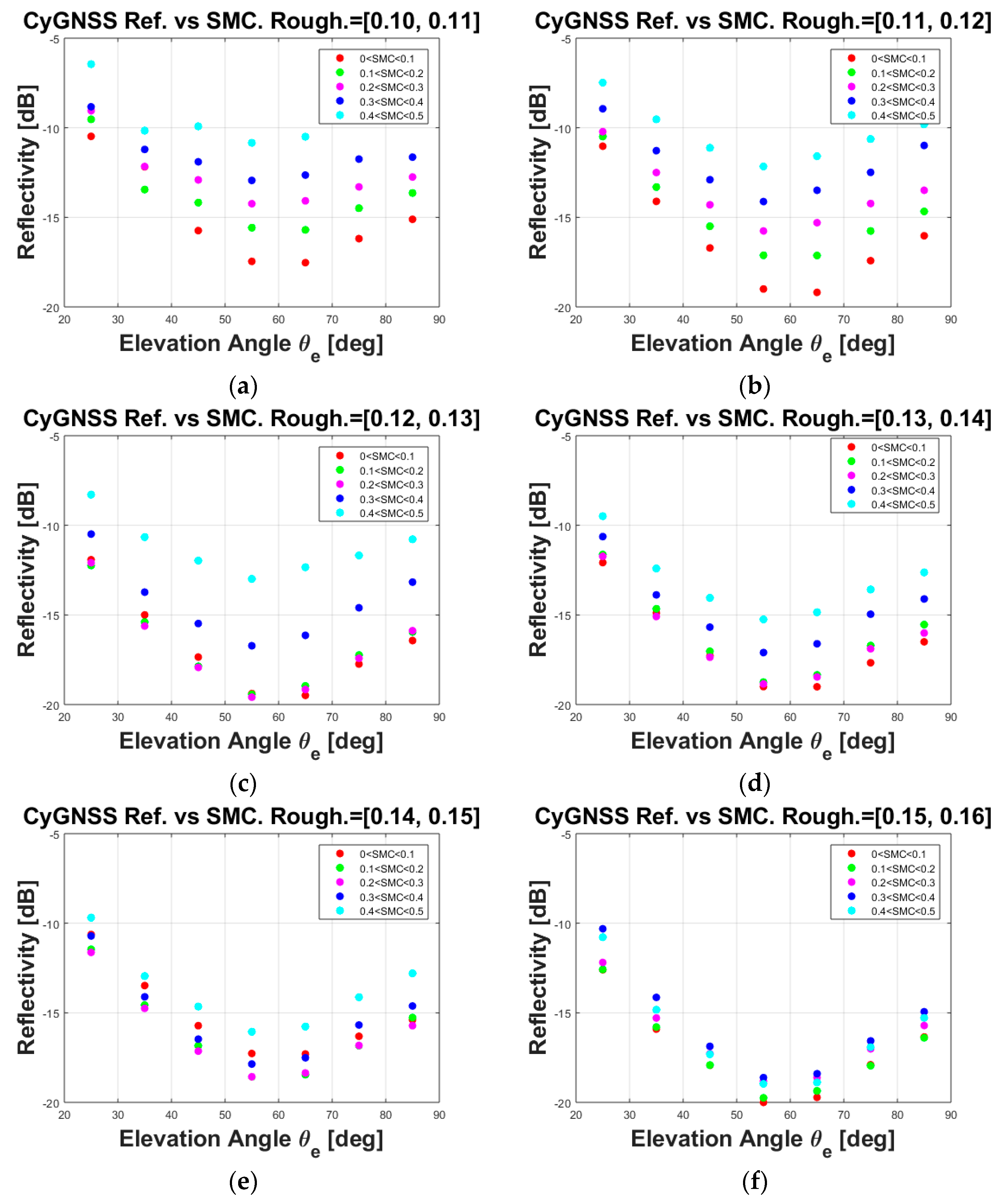
6.1. Global Analysis

The angular evolution of ${\mathsf{\Gamma }}_{\mathrm{L}\mathrm{H}\mathrm{C}\mathrm{P},\mathrm{C}\mathrm{y}\mathrm{G}\mathrm{N}\mathrm{S}\mathrm{S}}$ was studied averaging at steps of ${\mathsf{\theta }}_{\mathrm{e}}$ = 10° from ${\mathsf{\theta }}_{\mathrm{e}}$ = 20° to ${\mathsf{\theta }}_{\mathrm{e}}$ = 90° using different ranges of $\mathrm{h}$ (Figure 4a) and SMC (Figure 4b). The averaging was performed using data from the eight satellites of the CyGNSS constellation (the maximum of eight different DDMs were used in the averaging). The rate of change of ${\mathsf{\Gamma }}_{\mathrm{L}\mathrm{H}\mathrm{C}\mathrm{P},\mathrm{C}\mathrm{y}\mathrm{G}\mathrm{N}\mathrm{S}\mathrm{S}}$ was larger as $\mathrm{h}$ increased. At the same time, the larger the roughness, the lower ${\mathsf{\Gamma }}_{\mathrm{L}\mathrm{H}\mathrm{C}\mathrm{P},\mathrm{C}\mathrm{y}\mathrm{G}\mathrm{N}\mathrm{S}\mathrm{S}}$ was at all the selected SMC levels (Figure 5). Figure 5 also shows two differentiated ${\mathsf{\Gamma }}_{\mathrm{L}\mathrm{H}\mathrm{C}\mathrm{P},\mathrm{C}\mathrm{y}\mathrm{G}\mathrm{N}\mathrm{S}\mathrm{S}}$ angular ranges: ${\mathsf{\Gamma }}_{\mathrm{L}\mathrm{H}\mathrm{C}\mathrm{P},\mathrm{C}\mathrm{y}\mathrm{G}\mathrm{N}\mathrm{S}\mathrm{S}}$ decreased from ${\mathsf{\theta }}_{\mathrm{e}}$ ≈ 85° to ${\mathsf{\theta }}_{\mathrm{e}}$ ≈ 55°, and it increased from ${\mathsf{\theta }}_{\mathrm{e}}$ ≈ 55° to ${\mathsf{\theta }}_{\mathrm{e}}$ ≈ 25°. ${\mathsf{\Gamma }}_{\mathrm{L}\mathrm{H}\mathrm{C}\mathrm{P},\mathrm{C}\mathrm{y}\mathrm{G}\mathrm{N}\mathrm{S}\mathrm{S}}$ included contributions from both coherent and incoherent scattering regimes in both angular ranges. The main difference between both scattering regimes was on the combination of the electromagnetic field vectors. ${\mathsf{\sigma }}_{\mathrm{L}\mathrm{H}\mathrm{C}\mathrm{P},\mathrm{c}\mathrm{o}\mathrm{h}}^0$ came from the coherent combination of the signals scattered on the individual facets within the first Fresnel zone. ${\mathsf{\sigma }}_{\mathrm{L}\mathrm{H}\mathrm{C}\mathrm{P},\mathrm{i}\mathrm{n}\mathrm{c}\mathrm{o}\mathrm{h}}^0$ was the result of the random combination of electromagnetic waves coming from other scatterers within the glistening zone that added together at the receiving antenna. If the combination was totally coherent, ${\mathsf{\Gamma }}_{\mathrm{L}\mathrm{H}\mathrm{C}\mathrm{P},\mathrm{c}\mathrm{o}\mathrm{h}}$ accounted for all the reflected power. In the case of diffuse scattering, the random signs of the electric field cross-products cancelled out ${\mathsf{\sigma }}_{\mathrm{L}\mathrm{H}\mathrm{C}\mathrm{P},\mathrm{c}\mathrm{o}\mathrm{h}}^0$, and the reflected power was given by ${\mathsf{\sigma }}_{\mathrm{L}\mathrm{H}\mathrm{C}\mathrm{P},\mathrm{i}\mathrm{n}\mathrm{c}\mathrm{o}\mathrm{h}}^0$. The changes on the angular evolution of ${\mathsf{\Gamma }}_{\mathrm{L}\mathrm{H}\mathrm{C}\mathrm{P},\mathrm{C}\mathrm{y}\mathrm{G}\mathrm{N}\mathrm{S}\mathrm{S}}$ depended on the dominant scattering mechanism. In the interpretation of Figure 5 it should be considered that the averaging of the reflectivity was performed over the complete land-surface coverage enabled by CyGNSS, including bare soil, deserts, rough topography areas, and highly vegetated areas such as rainforests. As such, these results provide the average response of ${\mathsf{\Gamma }}_{\mathrm{L}\mathrm{H}\mathrm{C}\mathrm{P},\mathrm{C}\mathrm{y}\mathrm{G}\mathrm{N}\mathrm{S}\mathrm{S}}$ as a function of ${\mathsf{\theta }}_{\mathrm{e}}$.

${\mathsf{\Gamma }}_{\mathrm{L}\mathrm{H}\mathrm{C}\mathrm{P},\mathrm{C}\mathrm{y}\mathrm{G}\mathrm{N}\mathrm{S}\mathrm{S}}$ decreased in the first range (from ${\mathsf{\theta }}_{\mathrm{e}}$ ≈ 85° to ${\mathsf{\theta }}_{\mathrm{e}}$ ≈ 55°) because the incoherent scattering was dominant over the coherent one. The coherent integration time ${\mathrm{T}}_{\mathrm{c}}$ is an important parameter that influences the ratio of the coherent-to-incoherent scattering components, and in this experiment it was set to ${\mathrm{T}}_{\mathrm{c}}$ = 1 ms. A longer ${\mathrm{T}}_{\mathrm{c}}$ would limit the incoherent scattering term, so as to increase the coherent-to-incoherent ratio because it would better filter out the noise and the volume scattering term [32]. Previous research activities also found a transition from an incoherent to coherent scattering regime over the ocean surface [42,51], where ${\mathsf{\Gamma }}_{\mathrm{L}\mathrm{H}\mathrm{C}\mathrm{P},\mathrm{i}\mathrm{n}\mathrm{c}\mathrm{o}\mathrm{h}}$ is dominant for high ${\mathsf{\theta }}_{\mathrm{e}}$ [52]. Theoretical simulations were performed in Reference [52] to study the evolution of the incoherent reflected power as a function of ${\mathsf{\theta }}_{\mathrm{e}}$. It was found ${\mathrm{Y}}_{\mathrm{r},\mathrm{P}\mathrm{e}\mathrm{a}\mathrm{k},\mathrm{L}\mathrm{H}\mathrm{C}\mathrm{P}}$ decreased ≈ 20% when ${\mathsf{\theta }}_{\mathrm{e}}$ reduced from ${\mathsf{\theta }}_{\mathrm{e}}$ = 90° to ${\mathsf{\theta }}_{\mathrm{e}}$ = 50°.

${\mathsf{\Gamma }}_{\mathrm{L}\mathrm{H}\mathrm{C}\mathrm{P},\mathrm{C}\mathrm{y}\mathrm{G}\mathrm{N}\mathrm{S}\mathrm{S}}$ increased in the second range (from ${\mathsf{\theta }}_{\mathrm{e}}$ ≈ 55° to ${\mathsf{\theta }}_{\mathrm{e}}$ ≈ 25°), which could be justified because the reflectivity became mostly coherent ${\mathsf{\Gamma }}_{\mathrm{L}\mathrm{H}\mathrm{C}\mathrm{P},\mathrm{c}\mathrm{o}\mathrm{h}}$ in regions without rough topography. ${\mathsf{\sigma }}_{\mathrm{L}\mathrm{H}\mathrm{C}\mathrm{P},\mathrm{c}\mathrm{o}\mathrm{h}}^0$ was high over smooth or slightly-to-moderate rough surfaces, because it increased with a decrease in surface roughness. As such, ${\mathsf{\Gamma }}_{\mathrm{L}\mathrm{H}\mathrm{C}\mathrm{P},\mathrm{C}\mathrm{y}\mathrm{G}\mathrm{N}\mathrm{S}\mathrm{S}}$ increased with a decrease in ${\mathsf{\theta }}_{\mathrm{e}}$ in the angular range ${\mathsf{\theta }}_{\mathrm{e}}$ < 55° because the signal coherence increased with a decrease in ${\mathsf{\theta }}_{\mathrm{e}}$ [51], and thus ${\mathsf{\sigma }}_{\mathrm{L}\mathrm{H}\mathrm{C}\mathrm{P},\mathrm{c}\mathrm{o}\mathrm{h}}^0$ became dominant for ${\mathsf{\theta }}_{\mathrm{e}}$ < 55°. The scattering phenomenon became more complicated in regions with a rough topography. As such, this result should be understood as the average response over the Earth’s surface. For higher ${\mathsf{\theta }}_{\mathrm{e}}$, even in a Nadir-looking configuration, there was still a non-negligible coherent component so as to be tracked [32,53,54].

The dynamic range of ${\mathsf{\Gamma }}_{\mathrm{L}\mathrm{H}\mathrm{C}\mathrm{P},\mathrm{C}\mathrm{y}\mathrm{G}\mathrm{N}\mathrm{S}\mathrm{S}}$ was higher for lower roughness levels, which seemed to indicate GNSS-R loses sensitivity to SMC over rougher surfaces in a general scenario. This reduction of the dynamic range appeared to be dependent on ${\mathsf{\theta }}_{\mathrm{e}}$ along the second angular range, where ${\mathsf{\sigma }}_{\mathrm{L}\mathrm{H}\mathrm{C}\mathrm{P},\mathrm{c}\mathrm{o}\mathrm{h}}^0$ was dominant. This increment was larger for decreasing SMC levels, which meant that the effect of a higher signal coherence was more relevant over areas with low SMC. Additionally, the effect of a larger signal attenuation through the canopy layer ${\mathrm{L}}^{\mathrm{c}\mathrm{a}\mathrm{n}\mathrm{o}\mathrm{p}\mathrm{y}}$ over highly vegetated areas was larger for a lower ${\mathsf{\theta }}_{\mathrm{e}}$, which could contribute to this loss of sensitivity. Overall, ${\mathsf{\Gamma }}_{\mathrm{L}\mathrm{H}\mathrm{C}\mathrm{P},\mathrm{C}\mathrm{y}\mathrm{G}\mathrm{N}\mathrm{S}\mathrm{S}}$ increased as SMC increased for a given ${\mathsf{\theta }}_{\mathrm{e}}$ and $\mathrm{h}$ (Figure 5).

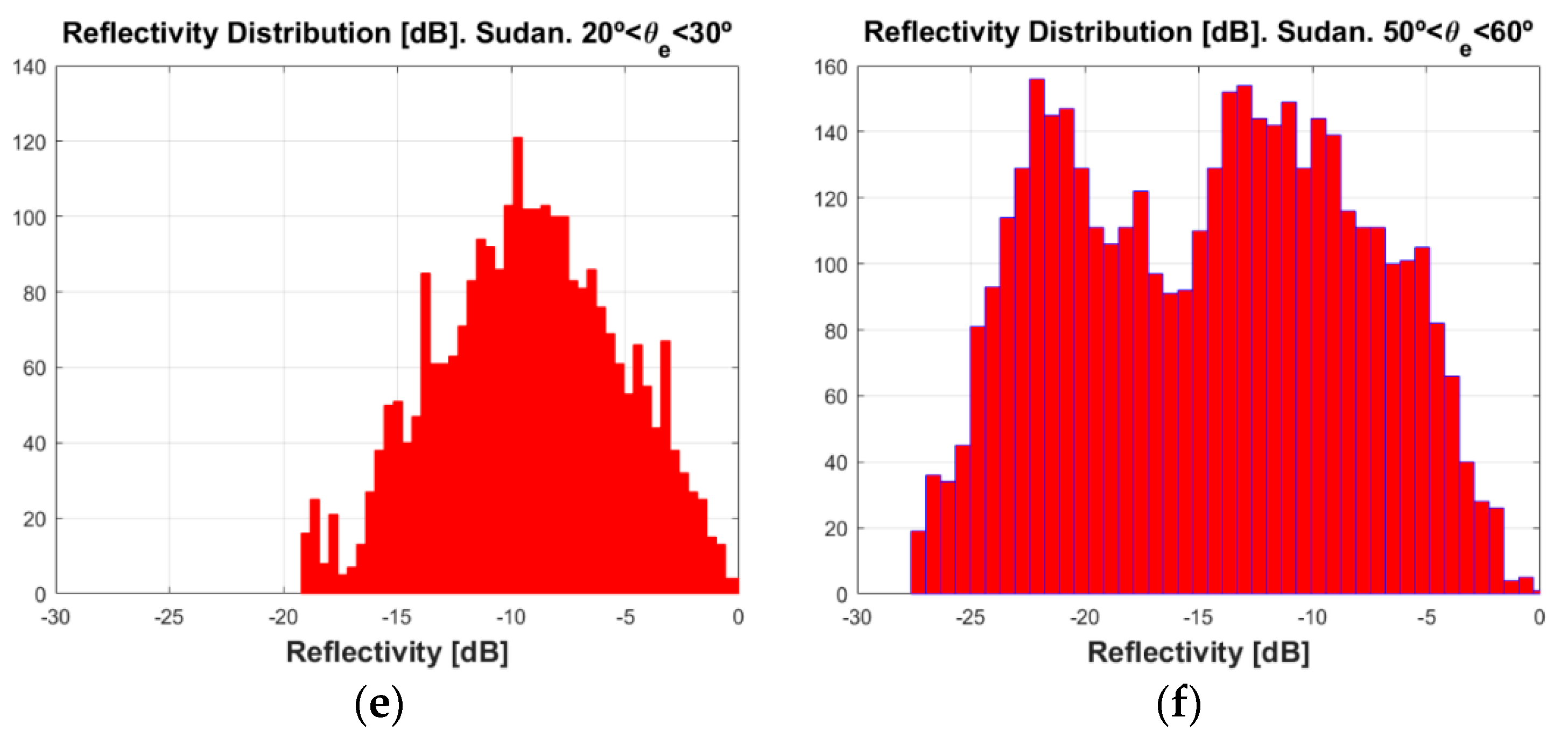
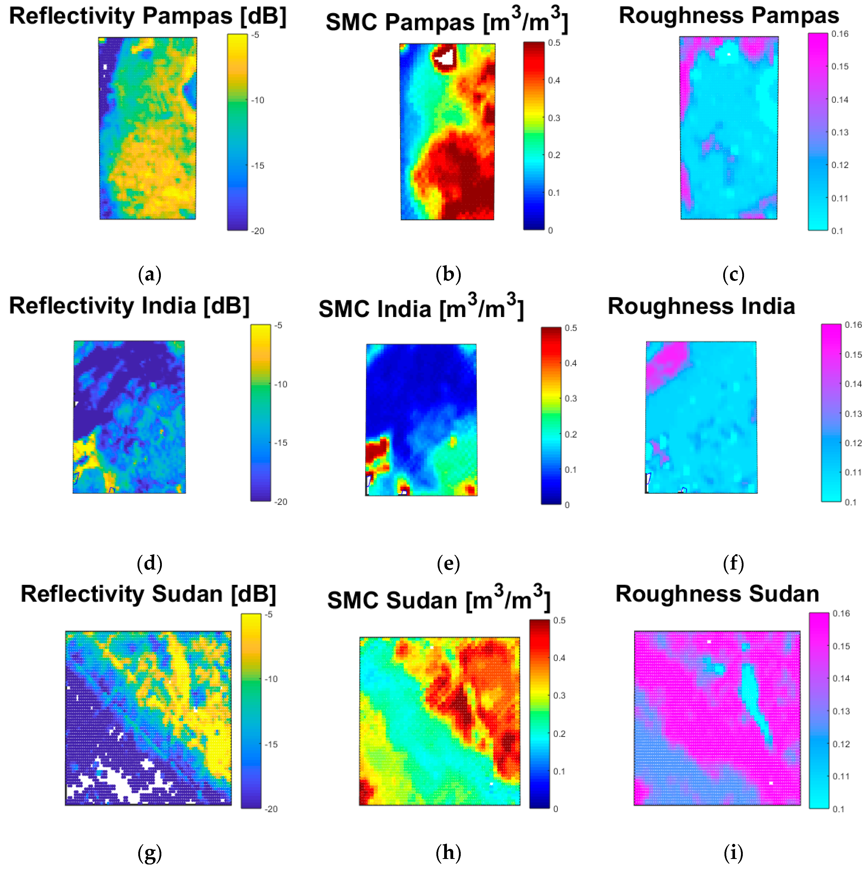
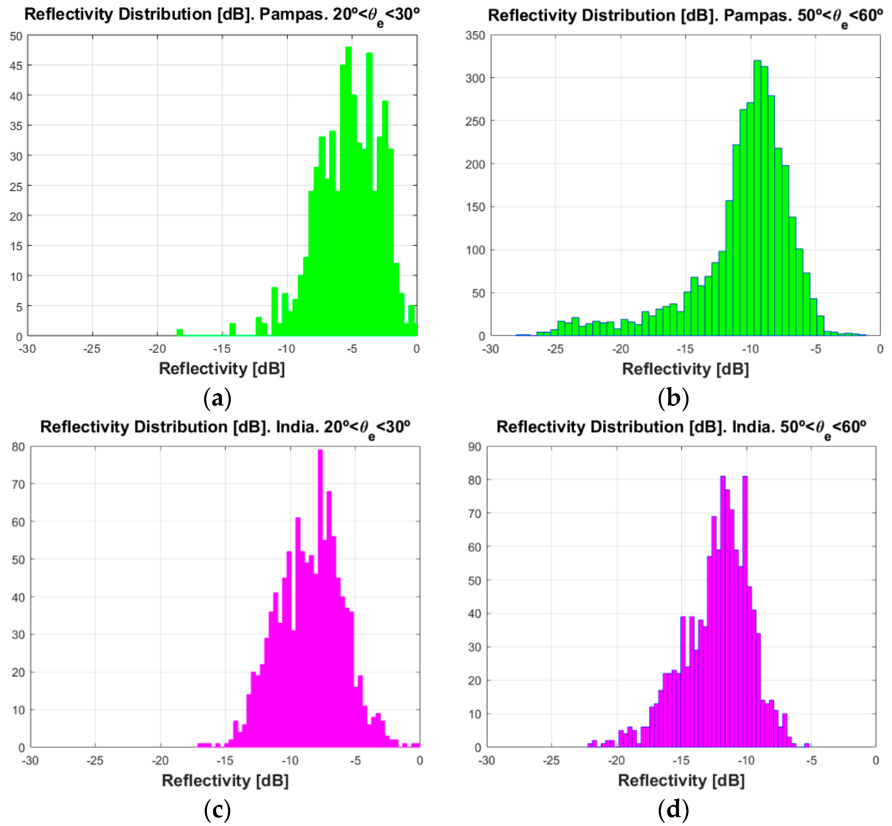
6.2. Regional Case Studies

Specific target areas with little vegetation over Argentina, India, and Sudan (Figure 6, Figure 7 and Figure 8) were selected for this section because they allowed for the evaluation of the impact of SMC and $\mathrm{h}$ in the angular evolution of ${\mathsf{\Gamma }}_{\mathrm{L}\mathrm{H}\mathrm{C}\mathrm{P},\mathrm{C}\mathrm{y}\mathrm{G}\mathrm{N}\mathrm{S}\mathrm{S}}$, excluding the effects of rough topography and high vegetation. The coordinates of these target areas are the following ones: Argentinian Pampas (Lat = [−37,−30]°, Lon = [−65,−60]°), India (Lat = [22,29]°, Lon = [70,77]°) and Sudan (Lat = [4,10]°, Lon = [25,33]°). The land cover-types were croplands (Pampas and India) and savannahs (Sudan), where the signal penetration depth was high, so as to minimize the vegetation effects. The Pearson correlation coefficient $\mathrm{r}$ of ${\mathsf{\Gamma }}_{\mathrm{L}\mathrm{H}\mathrm{C}\mathrm{P},\mathrm{C}\mathrm{y}\mathrm{G}\mathrm{N}\mathrm{S}\mathrm{S}}$ and SMC was calculated for each target area at steps of ${\mathsf{\theta }}_{\mathrm{e}}$ = 10° from ${\mathsf{\theta }}_{\mathrm{e}}$ = 20° to ${\mathsf{\theta }}_{\mathrm{e}}$ = 90° (

Table 2. Pearson correlation coefficients of CyGNSS reflectivity ${\mathsf{\Gamma }}_{\mathrm{L}\mathrm{H}\mathrm{C}\mathrm{P},\mathrm{C}\mathrm{y}\mathrm{G}\mathrm{N}\mathrm{S}\mathrm{S}}$ and SMAP-derived soil moisture content (SMC) for different elevation angles ${\mathsf{\theta }}_{\mathrm{e}}$, over specific target areas: Argentinian Pampas, India, and Sudan.

${\mathsf{\theta }}_{\mathbf{e}}$	Pampas	India	Sudan
[80,90]°	0.73	0.62	0.68
[70,80]°	0.77	0.68	0.69
[60,70]°	0.78	0.71	0.68
[50,60]°	0.76	0.72	0.65
[40,50]°	0.71	0.72	0.68
[30,40]°	0.60	0.70	0.74
[20,30]°	0.36	0.62	0.67

). The maximum Pearson coefficients ${\mathrm{r}}_{\mathrm{P}\mathrm{a}\mathrm{m}\mathrm{p}\mathrm{a}\mathrm{s}}$ ≈ 0.78, ${\mathrm{r}}_{\mathrm{I}\mathrm{n}\mathrm{d}\mathrm{i}\mathrm{a}}$ ≈ 0.72, and ${\mathrm{r}}_{\mathrm{S}\mathrm{u}\mathrm{d}\mathrm{a}\mathrm{n}}$ ≈ 0.74 were found, respectively, at ${\mathsf{\theta }}_{\mathrm{e}}$ ≈ [60,70]° and ${\mathrm{h}}_{\mathrm{P}\mathrm{a}\mathrm{m}\mathrm{p}\mathrm{a}\mathrm{s}}$ ≈ 0.1, ${\mathsf{\theta }}_{\mathrm{e}}$ ≈ [50,60]° and ${\mathrm{h}}_{\mathrm{I}\mathrm{n}\mathrm{d}\mathrm{i}\mathrm{a}}$ ≈ 0.11, and ${\mathsf{\theta }}_{\mathrm{e}}$ ≈ [30,40]° and ${\mathrm{h}}_{\mathrm{S}\mathrm{u}\mathrm{d}\mathrm{a}\mathrm{n}}$ ≈ 0.15. These coefficients were gradually achieved at lower ${\mathsf{\theta }}_{\mathrm{e}}$ for increasing mean values of $\mathrm{h}$ over these target areas. As such, the angular ranges associated with an improved correlation coefficient depend on $\mathrm{h}$. A lower ${\mathsf{\theta }}_{\mathrm{e}}$ was required to increase the signal coherence with an increase in $\mathrm{h}$, in agreement with the Rayleigh criterion that establishes a surface (without vegetation and without rough topography) could be considered smooth if the phase difference between two reflected electromagnetic waves was lower than π/2 rad:

$${\mathsf{\sigma }}_{\mathrm{R}\mathrm{M}\mathrm{S}}<\frac{\mathsf{\lambda }}{8\sin {\mathsf{\theta }}_{\mathrm{e}}}$$

(6)

where $\mathsf{\lambda }$ was the signal wavelength that at the L-band was ≈20 cm.

The angular dependence seemed to be lower over the Sudan target area (savannahs), which was characterized by a significantly higher effective surface roughness parameter. In this situation, ${\mathsf{\sigma }}_{\mathrm{L}\mathrm{H}\mathrm{C}\mathrm{P},\mathrm{i}\mathrm{n}\mathrm{c}\mathrm{o}\mathrm{h}}^0$ was high even for low ${\mathsf{\theta }}_{\mathrm{e}}$ and thus the power fluctuations of ${\mathrm{Y}}_{\mathrm{r},\mathrm{P}\mathrm{e}\mathrm{a}\mathrm{k},\mathrm{L}\mathrm{H}\mathrm{C}\mathrm{P}}$ were more linked to the size of the first iso-delay ellipse (much larger than that of the first Fresnel zone), which minimized the impact of ${\mathsf{\theta }}_{\mathrm{e}}$. Nonetheless, there was a non-negligible increment of the correlation for ${\mathsf{\theta }}_{\mathrm{e}}$ ≈ [30,40]°. The impact of ${\mathsf{\theta }}_{\mathrm{e}}$ was clearer over Argentinian Pampas and India (croplands). This experimental evidence was a symptom that over smoother surfaces (e.g., croplands), the correlation of ${\mathsf{\Gamma }}_{\mathrm{L}\mathrm{H}\mathrm{C}\mathrm{P},\mathrm{C}\mathrm{y}\mathrm{G}\mathrm{N}\mathrm{S}\mathrm{S}}$ and SMC was improved when the coherent scattering regime started to be the dominant one because: (a) A higher spatial resolution (smaller first Fresnel zone), as compared to that at lower ${\mathsf{\theta }}_{\mathrm{e}}$, minimized the effects of land cover heterogeneity (

Table 3. Size of the semi-major and semi-minor axis of the first Fresnel zone for the CyGNSS scenario, as a function of the elevation angle ${\mathsf{\theta }}_{\mathrm{e}}$.

${\mathsf{\theta }}_{\mathbf{e}}$	Semi-Minor Axes [m]	Semi-Major Axes [m]
90°	311	311
80°	313	317
70°	321	341
60°	334	385
50°	355	463
40°	388	603
30°	440	880
20°	532	1555

). (b) ${\mathsf{\sigma }}_{\mathrm{L}\mathrm{H}\mathrm{C}\mathrm{P},\mathrm{c}\mathrm{o}\mathrm{h}}^0$ was mainly related to surface scattering. The use of a higher ${\mathrm{T}}_{\mathrm{c}}$ would improve the sensitivity of GNSS-R to SMC [16] because it would filter out the power fluctuations linked to the incoherent scattering term.

The sensitivity to SMC was based on the difference between the dielectric properties of water and soil. Here, the sensitivity of ${\mathsf{\Gamma }}_{\mathrm{L}\mathrm{H}\mathrm{C}\mathrm{P},\mathrm{C}\mathrm{y}\mathrm{G}\mathrm{N}\mathrm{S}\mathrm{S}}$ to SMC was analyzed over these selected target areas (Figure 6a–f). In so doing, the selected ${\mathsf{\theta }}_{\mathrm{e}}$ ranges corresponded to those with the maximum Pearson correlation coefficient between ${\mathsf{\Gamma }}_{\mathrm{L}\mathrm{H}\mathrm{C}\mathrm{P},\mathrm{C}\mathrm{y}\mathrm{G}\mathrm{N}\mathrm{S}\mathrm{S}}$ and SMC (Table 2). Figure 6a,c,e shows the scatter plots of ${\mathsf{\Gamma }}_{\mathrm{L}\mathrm{H}\mathrm{C}\mathrm{P},\mathrm{C}\mathrm{y}\mathrm{G}\mathrm{N}\mathrm{S}\mathrm{S}}$ and SMC as a function of different $\mathrm{h}$ levels. Land cover-types over Pampas and India were croplands with moderate mean roughness: ${\mathrm{h}}_{\mathrm{P}\mathrm{a}\mathrm{m}\mathrm{p}\mathrm{a}\mathrm{s}}$ ≈ 0.1 (Figure 6b) and ${\mathrm{h}}_{\mathrm{I}\mathrm{n}\mathrm{d}\mathrm{i}\mathrm{a}}$ ≈ 0.11 (Figure 6d). The mean roughness over Sudan was higher: ${\mathrm{h}}_{\mathrm{S}\mathrm{u}\mathrm{d}\mathrm{a}\mathrm{n}}$ ≈ 0.15 (Figure 6f). The slopes of the linear regressions were ≈26 dB/(m³/m³), ≈37 dB/(m³/m³), and ≈50 dB/(m³/m³) respectively over the target areas, while the RMSE was ≈2.5 dB, ≈3 dB and ≈3.3 dB. In Sudan there was a smaller SMC variability and a significant dynamic range (Figure 6e). This explained the higher slope of the fit. On the other hand, the higher roughness $\mathrm{h}$ explained the higher RMSE and SD (

Table 4. Statistics (mean, standard deviation SD, kurtosis, and skewness) of the CyGNSS reflectivity ${\mathsf{\Gamma }}_{\mathrm{L}\mathrm{H}\mathrm{C}\mathrm{P},\mathrm{C}\mathrm{y}\mathrm{G}\mathrm{N}\mathrm{S}\mathrm{S}}$ distributions over the selected target areas (Argentinian Pampas, India, and Sudan).

	Pampas	India	Sudan
Mean [dB];${\mathsf{\theta }}_{\mathrm{e}}$ = [50,60]°	−10.6	−12.2	−14.5
Mean [dB];${\mathsf{\theta }}_{\mathrm{e}}$ = [20,30]°	−5.2	−8.4	−9.2
SD [dB];${\mathsf{\theta }}_{\mathrm{e}}$ = [50,60]°	3.9	2.5	6.4
SD [dB];${\mathsf{\theta }}_{\mathrm{e}}$ = [20,30]°	2.5	2.5	4
Kurtosis;${\mathsf{\theta }}_{\mathrm{e}}$ = [50,60]°	5.8	3.5	1.96
Kurtosis;${\mathsf{\theta }}_{\mathrm{e}}$ = [20,30]°	4.1	2.8	2.5
Skewness;${\mathsf{\theta }}_{\mathrm{e}}$ = [50,60]°	−1.5	−0.6	0
Skewness;${\mathsf{\theta }}_{\mathrm{e}}$ = [20,30]°	−0.5	0	−0.1

). Overall, a good sensitivity of ${\mathsf{\Gamma }}_{\mathrm{L}\mathrm{H}\mathrm{C}\mathrm{P},\mathrm{C}\mathrm{y}\mathrm{G}\mathrm{N}\mathrm{S}\mathrm{S}}$ to SMC was found over the three selected target areas. Figure 6b,d,f is useful to further understand the impact of $\mathrm{h}$ on the sensitivity to SMC [Pampas (Figure 6a), India (Figure 6c), and Sudan (Figure 6e)]. ${\mathsf{\Gamma }}_{\mathrm{L}\mathrm{H}\mathrm{C}\mathrm{P},\mathrm{C}\mathrm{y}\mathrm{G}\mathrm{N}\mathrm{S}\mathrm{S}}$ decreased with an increase in $\mathrm{h}$ for nearly constant levels of SMC, and at the same time this rate of change depended on the mean SMC level. For lower SMC levels, ${\mathsf{\Gamma }}_{\mathrm{L}\mathrm{H}\mathrm{C}\mathrm{P},\mathrm{C}\mathrm{y}\mathrm{G}\mathrm{N}\mathrm{S}\mathrm{S}}$ decreased significantly for a high $\mathrm{h}$ parameter, while ${\mathsf{\Gamma }}_{\mathrm{L}\mathrm{H}\mathrm{C}\mathrm{P},\mathrm{C}\mathrm{y}\mathrm{G}\mathrm{N}\mathrm{S}\mathrm{S}}$ appeared to be roughly independent of $\mathrm{h}$ for higher levels of SMC.

The histograms of ${\mathsf{\Gamma }}_{\mathrm{L}\mathrm{H}\mathrm{C}\mathrm{P},\mathrm{C}\mathrm{y}\mathrm{G}\mathrm{N}\mathrm{S}\mathrm{S}}$ over these target areas are displayed to complement the observations on the correlation coefficients (Figure 7). The corresponding statistics are also included in Table 4. Significant changes on the histograms were found from ${\mathsf{\theta }}_{\mathrm{e}}$ ≈ [20,30]° (Figure 7a,c,e) to ${\mathsf{\theta }}_{\mathrm{e}}$ ≈ [50,60]° (Figure 7b,d,f). The lowest mean ${\mathsf{\Gamma }}_{\mathrm{L}\mathrm{H}\mathrm{C}\mathrm{P},\mathrm{C}\mathrm{y}\mathrm{G}\mathrm{N}\mathrm{S}\mathrm{S}}$ and the highest standard deviation (SD) of the three target areas appeared over Sudan (Table 4). In this sense, it seems reasonable that the maximum correlation in Sudan was achieved over a significantly lower ${\mathsf{\theta }}_{\mathrm{e}}$ as compared to the Argentinian Pampas and India. A lower angular range was required to achieve a high enough signal coherence. A bimodal distribution (Figure 7f) was found over Sudan at ${\mathsf{\theta }}_{\mathrm{e}}$ ≈ [50,60]°, which was an additional factor that justified the lower angular variability over this particular target area (Table 2). The impact of a lower ${\mathsf{\theta }}_{\mathrm{e}}$ was quite evident in Figure 7e where the ${\mathsf{\Gamma }}_{\mathrm{L}\mathrm{H}\mathrm{C}\mathrm{P},\mathrm{C}\mathrm{y}\mathrm{G}\mathrm{N}\mathrm{S}\mathrm{S}}$ distribution turned into a unimodal one with a kurtosis ≈2.5, which tended to be like a Gaussian one. This indicated the presence of a coherent component in the total scattered electromagnetic field [15], and thus it is reasonable that the maximum correlation also appeared at this angular range. Over the Argentinian Pampas, the mean ${\mathsf{\Gamma }}_{\mathrm{L}\mathrm{H}\mathrm{C}\mathrm{P},\mathrm{C}\mathrm{y}\mathrm{G}\mathrm{N}\mathrm{S}\mathrm{S}}$ was higher than over India, and thus the maximum correlation appeared over a slightly higher ${\mathsf{\theta }}_{\mathrm{e}}$. For very low ${\mathsf{\theta }}_{\mathrm{e}}$ ≈ [20,30]°, the Pearson coefficients tended to decreases in all the selected target areas (Table 2), and this could be attributed to the lower ${\mathsf{\Gamma }}_{\mathrm{L}\mathrm{H}\mathrm{C}\mathrm{P},\mathrm{C}\mathrm{y}\mathrm{G}\mathrm{N}\mathrm{S}\mathrm{S}}$ dynamic range over this angular range.

${\mathsf{\Gamma }}_{\mathrm{L}\mathrm{H}\mathrm{C}\mathrm{P},\mathrm{C}\mathrm{y}\mathrm{G}\mathrm{N}\mathrm{S}\mathrm{S}}$, SMC, and $\mathrm{h}$ were geolocated over the specific target areas (Figure 8a–i) to further understand the effects of $\mathrm{h}$ on SMC estimation using GNSS-R. The averaged ${\mathsf{\Gamma }}_{\mathrm{L}\mathrm{H}\mathrm{C}\mathrm{P},\mathrm{C}\mathrm{y}\mathrm{G}\mathrm{N}\mathrm{S}\mathrm{S}}$ over Argentinian Pampas is shown in Figure 8a. The spatial pattern was clearly correlated with that of the SMAP-derived SMC (Figure 8b), which appeared to be the most important parameter. However, the impact of $\mathrm{h}$ was also relevant, especially on the upper-right side of Figure 8a–c. In this area, there was a sudden drop of $\mathrm{h}$ that enabled an increment of ${\mathsf{\Gamma }}_{\mathrm{L}\mathrm{H}\mathrm{C}\mathrm{P},\mathrm{C}\mathrm{y}\mathrm{G}\mathrm{N}\mathrm{S}\mathrm{S}}$ for nearly constant values of SMC. The spatial variability of ${\mathsf{\Gamma }}_{\mathrm{L}\mathrm{H}\mathrm{C}\mathrm{P},\mathrm{C}\mathrm{y}\mathrm{G}\mathrm{N}\mathrm{S}\mathrm{S}}$ was higher than radiometer data because of the higher resolution of GNSS-R, which was associated with the size of first Fresnel zone.

The target area over India was selected because this was a relatively dry region with some SMC peaks, so as to complement the information obtained from the wet Argentinian Pampas. ${\mathsf{\Gamma }}_{\mathrm{L}\mathrm{H}\mathrm{C}\mathrm{P},\mathrm{C}\mathrm{y}\mathrm{G}\mathrm{N}\mathrm{S}\mathrm{S}}$ increased due to a positive gradient on SMC. This effect was lower than over the Argentinian Pampas because of the reduced roughness range $\mathrm{h}$ < 0.13 as compared to that over the Argentinian Pampas $\mathrm{h}$< 0.16. This result agrees with the conclusions derived from Figure 6b,d,f, where the effect of surface roughness was shown to be more significant for $\mathrm{h}$ > 0.13.

Finally, the averaged ${\mathsf{\Gamma }}_{\mathrm{L}\mathrm{H}\mathrm{C}\mathrm{P},\mathrm{C}\mathrm{y}\mathrm{G}\mathrm{N}\mathrm{S}\mathrm{S}}$ over Sudan showed two clearly differentiated spatial patterns that corresponded to SMC levels from moderate (0.2 < SMC < 0.3) to very high (0.4 < SMC < 0.5). The down-left side highlights the effects of $\mathrm{h}$ on ${\mathsf{\Gamma }}_{\mathrm{L}\mathrm{H}\mathrm{C}\mathrm{P},\mathrm{C}\mathrm{y}\mathrm{G}\mathrm{N}\mathrm{S}\mathrm{S}}$ over an area with moderate SMC. Here, the surface roughness was also high $\mathrm{h}$ > 0.13, and thus ${\mathsf{\Gamma }}_{\mathrm{L}\mathrm{H}\mathrm{C}\mathrm{P},\mathrm{C}\mathrm{y}\mathrm{G}\mathrm{N}\mathrm{S}\mathrm{S}}$ holds quite low ≈ −20 dB despite the increment on SMC from ≈0.2 m³/m³ to ≈0.4 m³/m³.

7. Final Discussions

${\mathsf{\Gamma }}_{\mathrm{L}\mathrm{H}\mathrm{C}\mathrm{P},\mathrm{C}\mathrm{y}\mathrm{G}\mathrm{N}\mathrm{S}\mathrm{S}}$ and the sensitivity of ${\mathsf{\Gamma }}_{\mathrm{L}\mathrm{H}\mathrm{C}\mathrm{P},\mathrm{C}\mathrm{y}\mathrm{G}\mathrm{N}\mathrm{S}\mathrm{S}}$ to SMC appeared to have a dependence with ${\mathsf{\theta }}_{\mathrm{e}}$ through $\mathrm{h}$ since the effective surface roughness was an important parameter that determined the amount of reflected power. The use of the polarimetric ratio (ratio of the reflected signals’ power at two different polarizations) could provide a significant correction of $\mathrm{h}$ in SMC estimation, and potentially this technique could also be used in future missions, especially if daily/hourly SMC monitoring is required. On the other hand, further research is required in single-polarization missions. Multi-temporal techniques are based on change detection, under the assumption that surface roughness does not change over consecutive overpasses and thus the variability on the radar coefficient is due to SMC. However, this is partially realistic because [55]: (a) isolating SMC changes from other factors such as VWC would be difficult, and (b) the actual surface roughness has a dependence with SMC. Some different retrieval algorithms of SMC and surface roughness $\mathrm{h}$ are based on multi-angular information. This approach could be useful in the case of CyGNSS eight-microsatellite constellation mission. Results from this study show that GNSS-R had an optimum sensitivity to SMC at different ${\mathsf{\theta }}_{\mathrm{e}}$, depending on the roughness levels. As such, this relationship could be used to select the most appropriate angular range in SMC determination. On the other hand, this property can be exploited to mitigate roughness effects at an improved temporal resolution as compared to multi-temporal techniques. Additionally, the experimental results show that the coherently scattered electromagnetic field was higher than theoretical predictions. This is an important finding, which paves the way for SMC retrieval from nanosatellites because the coherent component was roughly independent of the platform’s height. Thus, relatively small antennas can be sufficient to obtain accurate measurements.

8. Conclusions

The impact of ${\mathsf{\theta }}_{\mathrm{e}}$ on CyGNSS GNSS-R bistatic reflectivity ${\mathsf{\Gamma }}_{\mathrm{L}\mathrm{H}\mathrm{C}\mathrm{P},\mathrm{C}\mathrm{y}\mathrm{G}\mathrm{N}\mathrm{S}\mathrm{S}}$ was assessed over the Earth’s surface with a focus on land as a function of soil moisture content (SMC) and effective surface roughness parameter $\mathrm{h}$. Global scale results show that ${\mathsf{\Gamma }}_{\mathrm{L}\mathrm{H}\mathrm{C}\mathrm{P},\mathrm{C}\mathrm{y}\mathrm{G}\mathrm{N}\mathrm{S}\mathrm{S}}$ decreased with decreasing ${\mathsf{\theta }}_{\mathrm{e}}$ down to ≈55° because of the effect of the incoherent scattering term ${\mathsf{\sigma }}_{\mathrm{L}\mathrm{H}\mathrm{C}\mathrm{P},\mathrm{i}\mathrm{n}\mathrm{c}\mathrm{o}\mathrm{h}}^0$. On the other hand, it increased for lower ${\mathsf{\theta }}_{\mathrm{e}}$. This could be explained because of a higher signal coherence that increased the coherent scattering term ${\mathsf{\sigma }}_{\mathrm{L}\mathrm{H}\mathrm{C}\mathrm{P},\mathrm{c}\mathrm{o}\mathrm{h}}^0$ in regions without a rough topography. This functional relationship depended on SMC and $\mathrm{h}$. Also at a global scale, it appeared that the dynamic range of ${\mathsf{\Gamma }}_{\mathrm{L}\mathrm{H}\mathrm{C}\mathrm{P},\mathrm{C}\mathrm{y}\mathrm{G}\mathrm{N}\mathrm{S}\mathrm{S}}$ at a fixed ${\mathsf{\theta }}_{\mathrm{e}}$ was higher as $\mathrm{h}$ decreased. The sensitivity of ${\mathsf{\Gamma }}_{\mathrm{L}\mathrm{H}\mathrm{C}\mathrm{P},\mathrm{C}\mathrm{y}\mathrm{G}\mathrm{N}\mathrm{S}\mathrm{S}}$ to SMC was then studied as a function of these two parameters for different sparsely vegetated target areas. The optimum Pearson correlation coefficients were found to be ${\mathrm{r}}_{\mathrm{P}\mathrm{a}\mathrm{m}\mathrm{p}\mathrm{a}\mathrm{s}}$ ≈ 0.78 at ${\mathsf{\theta }}_{\mathrm{e}}$ ≈ [60,70]°, ${\mathrm{r}}_{\mathrm{I}\mathrm{n}\mathrm{d}\mathrm{i}\mathrm{a}}$ ≈ 0.72 at ${\mathsf{\theta }}_{\mathrm{e}}$ ≈ [50,60]°, and ${\mathrm{r}}_{\mathrm{S}\mathrm{u}\mathrm{d}\mathrm{a}\mathrm{n}}$ ≈ 0.74 at ${\mathsf{\theta }}_{\mathrm{e}}$ ≈ [30,40]°, for different mean levels of roughness ${\mathrm{h}}_{\mathrm{P}\mathrm{a}\mathrm{m}\mathrm{p}\mathrm{a}\mathrm{s}}$ ≈ 0.1, ${\mathrm{h}}_{\mathrm{I}\mathrm{n}\mathrm{d}\mathrm{i}\mathrm{a}}$ ≈ 0.11, and ${\mathrm{h}}_{\mathrm{S}\mathrm{u}\mathrm{d}\mathrm{a}\mathrm{n}}$ ≈ 0.15. At these angular ranges, the slopes of the linear regressions over these target areas were ≈26 dB/(m³/m³), ≈37 dB/(m³/m³), and ≈50 dB/(m³/m³), respectively. The empirically-derived impact of ${\mathsf{\theta }}_{\mathrm{e}}$ on the relationship of ${\mathsf{\Gamma }}_{\mathrm{L}\mathrm{H}\mathrm{C}\mathrm{P},\mathrm{C}\mathrm{y}\mathrm{G}\mathrm{N}\mathrm{S}\mathrm{S}}$ with SMC and $\mathrm{h}$ could provide useful information in the development of first order corrections of surface roughness. As a final remark, a better sensitivity of GNSS-R to SMC appeared over croplands when the coherent scattering term ${\mathsf{\sigma }}_{\mathrm{L}\mathrm{H}\mathrm{C}\mathrm{P},\mathrm{c}\mathrm{o}\mathrm{h}}^0$ became dominant over the incoherent one ${\mathsf{\sigma }}_{\mathrm{L}\mathrm{H}\mathrm{C}\mathrm{P},\mathrm{i}\mathrm{n}\mathrm{c}\mathrm{o}\mathrm{h}}^0$. Therefore, SMC retrieval using GNSS-R could benefit on the higher spatial resolution of the coherent scattering regime, limited by the first Fresnel zone.

CyGNSS is a good example of how a constellation of small satellites could provide complementary information to a classical satellite such as SMAP, with a higher spatiotemporal sampling in the latitudinal band ≈ [–40,40]°. The revolution of small satellites, such as CubeSats, allowing for the provision of scientifically valuable data has just started. Future research on deployable antennas would provide a chance to elucidate whether such low-cost, small-size satellites could provide an accuracy on the same order than a classical satellite. On the other hand, passive microwave Earth observation techniques (e.g., microwave radiometry, GNSS-R) fit quite well on a single CubeSat [56], enabling the use of low power-consumption instruments that pave the way to improve the operational duty-cycle. As a matter of fact, the spatial resolution of GNSS-R is ≈1 km under the coherent scattering regime. This can clearly improve the resolution of microwave radiometry (SMAP) ≈40 km.

References

1. Poghosyan, A.; Golkar, A. CubeSat evolution: Analyzing CubeSat capabilities for conducting science missions. Elsevier Prog. Aerosp. Sci. 2017, 88, 59–83. [Google Scholar] [CrossRef]
2. Gleason, S.; Hodgart, S.; Sun, Y.; Gommenginger, C.; Mackin, S.; Adjrad, M.; Unwin, M. Detection and processing of bistatically reflected GPS signals from low Earth orbit for the purpose of ocean remote sensing. IEEE Trans. Geosci. Remote Sens. 2005, 43, 1229–1241. [Google Scholar] [CrossRef]
3. Unwin, M.; Jales, P.; Blunt, P.; Duncan, S. Preparation for the first flight of SSTL’s next generation space GNSS receivers. In Proceedings of the 6th ESA/European Workshop Satellite NAVITEC GNSS Signals Signal Processing, Noordwijk, The Netherlands, 5–7 December 2012; pp. 1–6. [Google Scholar]
4. Carreno-Luengo, H.; Camps, A.; Via, P.; Munoz, J.F.; Cortiella, A.; Vidal, D.; Jané, J.; Catarino, N.; Hagenfeldt, M.; Palomo, P.; et al. 3Cat-2—An experimental nanosatellite for GNSS-R earth observation: Mission concept and analysis. IEEE J. Sel. Top. Appl. Earth Obs. Remote Sens. 2016, 9, 4540–4551. [Google Scholar] [CrossRef]
5. Lowe, S.T.; LaBrecque, J.L.; Zuffada, C.; Romans, L.J.; Young, L.E.; Hajj, G.A. First spaceborne observation of an Earth-reflected GPS signal. Radio Sci. 2002, 37, 1–28. [Google Scholar] [CrossRef]
6. Martín-Neira, M.; Li, W.; Andrés-Beivide, A.; Ballesteros-Sels, X. Cookie: A satellite concept for GNSS remote sensing constellations. IEEE J. Sel. Top. Appl. Earth Obs. Remote Sens. 2016, 9, 4593–4610. [Google Scholar] [CrossRef]
7. Cardellach, E.; Wickert, J.; Baggen, R.; Benito, J.; Camps, A.; Catarino, N.; Chapron, B.; Dielacher, A.; Fabra, F.; Flato, G.; et al. GNSS Transpolar Earth Reflectometry exploring System (G-TERN): Mission concept. IEEE Trans. Geosci. Remote Sens. 2018, 6, 13980–14018. [Google Scholar] [CrossRef]
8. Martín-Neira, M.; D’Addio, S.; Buck, C.; Floury, M.; Prieto-Cerdeira, R. The PARIS ocean altimeter in-orbit demonstrator. IEEE Trans. Geosci. Remote Sens. 2011, 49, 2209–2237. [Google Scholar] [CrossRef]
9. Garrison, J.L.; Komjathy, A.; Zavorotny, V.U.; Katzberg, S.J. Wind speed measurement using forward scattered GPS signals. IEEE Trans. Geosci. Remote Sens. 2002, 40, 50–65. [Google Scholar] [CrossRef] [Green Version]
10. Zavorotny, V.U.; Larson, K.M.; Braun, J.J.; Small, E.E.; Gutmann, E.D.; Bilich, A.L. A physical model for GPS multipath caused by land reflections: Toward bare soil moisture retrievals. IEEE J. Sel. Top. Appl. Earth Obs. Remote Sens. 2009, 3, 100–110. [Google Scholar] [CrossRef]
11. Larson, K.M.; Small, E.E.; Gutmann, E.; Bilich, A.; Axelrad, P.; Braun, J. Using GPS multipath to measure soil moisture fluctuations: Initial results. GPS Solut. 2008, 12, 173–177. [Google Scholar] [CrossRef]
12. Ruf, C.; Unwin, M.; Dickinson, J.; Rose, R.; Rose, D.; Vincent, M.; Lyons, A. CYGNSS: Enabling the future of hurricane prediction [Remote Sensing Satellites]. IEEE Geosci. Remote Sens. Mag. 2016, 1, 52–67. [Google Scholar] [CrossRef]
13. Ruf, C.; Atlas, R.; Chang, P.; Clarizia, M.; Garrison, J.; Gleason, S.; Katzberg, S.; Jelenak, Z.; Johnson, J.; Majumdar, S.; et al. New ocean winds satellite mission to probe hurricanes and tropical convection. Bull. Am. Meteorol. Soc. 2015, 97, 385–395. [Google Scholar] [CrossRef]
14. Bussy-Virat, C.D.; Ruf, C.S.; Ridley, A.J. Relationship between temporal and spatial resolution for a constellation of GNSS-R satellites. IEEE J. Sel. Top. Appl. Earth Obs. Remote Sens. 2018. [Google Scholar] [CrossRef]
15. Egido, A.; Paloscia, S.; Motte, E.; Guerriero, L.; Pierdicca, N.; Vaparrini, M.; Santi, E.; Fontanelli, G.; Floury, N. Airborne GNSS-R polarimetric measurements for soil moisture and above ground biomass estimation. IEEE J. Sel. Top. Appl. Earth Obs. Remote Sens. 2014, 7, 1522–1532. [Google Scholar] [CrossRef]
16. Carreno-Luengo, H.; Lowe, S.T.; Zuffada, C.; Esterhuizen, S.; Oveisgharan, S. Spaceborne GNSS-R from the SMAP mission: First assessment of polarimetric scatterometry over land and cryosphere. Remote Sens. 2017, 9, 362. [Google Scholar] [CrossRef]
17. Chew, C.; Small, E.E. Soil moisture sensing using spaceborne GNSS reflections: Comparison of CYGNSS reflectivity to SMAP soil moisture. Geophys. Res. Lett. 2018, 45, 4049–4057. [Google Scholar] [CrossRef]
18. Wang, S.G.; Li, X.; Han, X.J.; Jin, R. Estimation of surface soil moisture and roughness from multi-angular ASAR imagery in the Watershed Allied Telemetry Experimental Research (WATER). Hydrol. Earth Syst. Sci. 2011, 15, 1415–1426. [Google Scholar] [CrossRef] [Green Version]
19. Shi, J.; Wang, J.; Hsu, A.Y.; O’Neill, P.E.; Engman, E. Estimation of bare surface soil moisture and surface roughness parameter using L-band SAR image SAR. IEEE Trans. Geosci. Remote Sens. 1997, 35, 1254–1266. [Google Scholar]
20. Pierdicca, N.; Pulvirenti, L.; Ticconi, F.; Brogioni, M. Radar bistatic configurations for soil moisture retrieval: a simulation study. IEEE Trans. Geosci. Remote Sens. 2008, 46, 3252–3264. [Google Scholar] [CrossRef]
21. Paloscia, S.; Pampaloni, P.; Chiaranti, L.; Coppo, P.; Gagliani, S.; Luzi, G. Multifrequency passive microwave remote sensing of soil moisture and roughness. Int. J. Remote Sens. 1991, 14, 467–483. [Google Scholar] [CrossRef]
22. Piles, M.; Camps, A.; Vall-llosera, M.; Monerris, A.; Talone, M.; Sabater, J.M. Performance of soil moisture retrieval algorithms using multiangular L band brightness temperatures. Water Resour. Res. 2010, 46, 1–9. [Google Scholar] [CrossRef]
23. Pierdicca, N.; Guerriero, L.; Brogioni, M.; Egido, A. On the coherent and non- coherent components of bare and vegetated terrain bistatic scattering: Modelling the GNSS-R signal over land. In Proceedings of the IEEE International Geoscience and Remote Sensing Symposium, Munich, Germany, 22–27 July 2012; pp. 3407–3410. [Google Scholar]
24. Martín, F.; Camps, A.; Martín-Neira, M.; D’Addio, S.; Fabra, F.; Rius, A.; Park, H. Impact of the elevation angle in the coherence time as a function of the sea wave height. In Proceedings of the IEEE International Geoscience and Remote Sensing Symposium, Milan, Italy, 26–31 July 2015; pp. 3630–3633. [Google Scholar]
25. CYGNSS. CYGNSS Level 1 Science Data Record Version 2.0. 2017. PO.DAAC, CA, USA. Available online: http://dx.doi.org/10.5067/CYGNS-L1X20 (accessed on 3 May 2018).
26. Masters, D.; Zavorotny, V.U.; Katzsberg, S.; Emery, W. GPS signal scattering from land for moisture content determination. In Proceedings of the IEEE International Geoscience and Remote Sensing Symposium, Honolulu, HI, USA, 24–28 July 2000; pp. 3090–3092. [Google Scholar]
27. Egido, A.; Martín-Puig, C.; Felip, D.; Garcia, M.; Caparrini, M.; Farrés, E.; Ruffini, G. The SAM sensor: An innovative GNSS-R system for soil moisture retrieval. In Proceedings of the NAVITEC Conference, European Space and Technology Centre in Noordwijk, Noordwijk, The Netherlands, 10–12 April 2008. [Google Scholar]
28. Katzberg, S.J.; Torres, O.; Grant, M.S.; Masters, D. Utilizing calibrated GPS reflected signals to estimate soil reflectivity and dielectric constant: Results from SMEX02. Remote Sens. Environ. 2006, 100, 17–28. [Google Scholar] [CrossRef] [Green Version]
29. Pierdicca, N.; Guerriero, L.; Giusto, R.; Brogioni, M.; Egido, A. SAVERS: A Simulator of GNSS Reflections from Bare and Vegetated Soils. IEEE Trans. Geosci. Remote Sens. 2014, 52, 6542–6554. [Google Scholar] [CrossRef]
30. Rodriguez-Alvarez, N.; Bosch-Lluis, X.; Camps, A.; Vall-llosera, M.; Valencia, E.; Marchan-Hernadez, J.F.; Ramos-Perez, I. Soil moisture retrieval using GNSS-R techniques: Experimental results over a bare soil feld. IEEE Trans. Geosci. Remote Sens. 2009, 47, 3616–3624. [Google Scholar] [CrossRef]
31. Alonso-Arroyo, A.; Camps, A.; Aguasca, A.; Forte, G.; Moneris, A.; Rudiger, C.; Walker, J.P.; Park, H.; Pacual, D.; Onrubia, R. Dual-Polarization GNSS-R Interference Pattern Technique for Soil Moisture Mapping. IEEE Trans. Geosci. Remote Sens. 2014, 7, 1533–1544. [Google Scholar] [CrossRef]
32. Carreno-Luengo, H.; Camps, A.; Querol, J.; Forte, G. First results of a GNSS-R experiment from a stratospheric balloon over boreal forests. IEEE Trans. Geosci. Remote Sens. 2015, 54, 2652–2663. [Google Scholar] [CrossRef]
33. Motte, E.; Zribi, M.; Fanise, P.; Egido, A.; Darrozes, J.; Al-Yaari, A.; Baghdadi, N.; Baup, F.; Dayau, S.; Fieuzal, R.; et al. GLORI: A GNSS-R dual polarization airborne instrument for land surface monitoring. Sensors 2016, 16, 732. [Google Scholar] [CrossRef] [PubMed] [Green Version]
34. Small, E.E.; Kristine, M.L.; Chew, C.C.; Dong, J.; Ochsner, T.E. Validation of GPS-IR soil moisture retrievals: Comparison of different algorithms to remove vegetation effects. IEEE Trans. Geosci. Remote Sens. 2016, 9, 4759–4770. [Google Scholar] [CrossRef]
35. Camps, A.; Hyuk, H.; Pablos, M.; Foti, G.; Gommerginger, C.P.; Liu, P.W.; Judge, J. Sensitivity of GNSS-R spaceborne observations to soil moisture and vegetation. IEEE Trans. Geosci. Remote Sens. 2016, 9, 4730–4732. [Google Scholar] [CrossRef]
36. Chew, C.; Shah, R.; Zuffada, Z.; Hajj, G.; Masters, D.; Mannucci, A.J. Demonstrating soil moisture remote sensing with observations from the UK TechDemoSat-1 satellite mission. Geophys. Res. Lett. 2016, 43, 3317–3324. [Google Scholar] [CrossRef]
37. Piles, M.; Entekhabi, D.; Konings, A.G.; McColl, K.A.; Das, N.N.; Jagdhuber, T. Multi-temporal microwave retrievals of soil moisture and vegetation parameters from SMAP. In Proceedings of the IEEE International Geoscience and Remote Sensing Symposium, Beijing, China, 10–15 July 2016; pp. 242–245. [Google Scholar]
38. Pierdicca, N.; Mollfulleda, A.; Martín, F.; Guerriero, L.; Paloscia, S.; Santi, E.; Floury, N. GNSS signal under forests for biomass retrieval: Experimental results and models. In Proceedings of the Specialist Meeting on Reflectometry Using GNSS and other Signals of Opportunity, University of Michigan, Ann Arbor, MI, USA, 23–25 May 2017; Available online: http://www.gnssr2017.org/workshop-program.html (accessed on 2 May 2018).
39. Peake, W.H. Interaction of electromagnetic waves with some natural surfaces. IEEE Trans. Antennas Propag. 1959, 7, 324–329. [Google Scholar] [CrossRef]
40. Tsang, L.; Newton, R.W. Microwave emissions from soils with rough surfaces. J. Geophys. Res. 1982, 87, 9017–9024. [Google Scholar] [CrossRef]
41. Zribi, M.; Baghdadi, N.; Guérin, C. Analysis of surface roughness heterogeneity and scattering behavior for radar measurements. IEEE Trans. Geosci. Remote Sens. 2006, 44, 2438–2444. [Google Scholar] [CrossRef]
42. Voronovich, A.G.; Zavorotny, V.U. Bistatic radar equation for signals of opportunity revisited. IEEE Trans. Geosci. Remote Sens. 2017, 56, 1959–1968. [Google Scholar] [CrossRef]
43. Carreno-Luengo, H.; Luzi, G.; Crosetto, M. Sensitivity of CyGNSS bistatic reflectivity and SMAP microwave brightness temperature to geophysical parameters over land surfaces. IEEE J. Sel. Top. Appl. Earth Obs. Remote Sens. 2018. [Google Scholar] [CrossRef]
44. Wang, J.R.; Schmugge, T.J. An empirical model for the complex dielectric permittivity of soils as a function of water content. IEEE Trans. Geosci. Remote Sens. 1980, 4, 288–295. [Google Scholar] [CrossRef]
45. Park, H.; Camps, A.; Pascual, D.; Alonso-Arroyo, A.; Querol, J.; Onrubia, R. Improvement of PAU/PARIS end-to-end performance simulator (P2PEPS): Land scattering including topography. In Proceedings of the IEEE International Geoscience and Remote Sensing Symposium, Beijing, China, 10–15 July 2016; pp. 5607–5610. [Google Scholar]
46. O’Neill, P.E.; Chan, S.; Njoku, E.G.; Jackson, T.; Bindlish, R. SMAP Enhanced L3 Radiometer Global Daily 9 km EASE-Grid Soil Moisture, Version 1; [SPL3SMP_E]; NASA National Snow Ice Data Center Distributed Active Archive Center: Boulder, CO, USA, 2016. [CrossRef]
47. Entekhabi, D.; Yueh, S.; O’Neill, P.E.; Kellogg, K.H.; Allen, A.; Bindlish, R.; Brown, M.; Chan, S.; Colliander, A.; Crow, W.; et al. SMAP Handbook. Soil Moisture Active Passive. Available online: https://nsidc.org/data/SPL3SMP_E/versions/1 (accessed on 6 April 2018).
48. O’Neill, P.E.; Chan, S.; Njoku, E.; Jackson, T.; Bindlish, R. Soil Moisture Active Passive (SMAP) Algorithm Theoretical Basis Document Level 2 & 3 Soil Moisture (Passive) Data Products. Revision C. December 2016. Available online: https://nsidc.org/data/SPL3SMP_E/versions/1 (accessed on 16 April 2018).
49. Koike, T.; Nakamura, Y.; Kaihotsu, I.; Davaa, G.; Matsuura, N.; Tamagawa, K.; Fujii, H. Development of an Advanced Microwave Scanning Radiometer (AMSR-E) algorithm of soil moisture and vegetation water content. Ann. J. Hydraul. Eng. Jpn. Soc. Civ. Eng. 2004, 48, 217–222. [Google Scholar] [CrossRef]
50. Hornbuckle, B.; Walker, V.; Eichinger, B.; Wallace, V.; Yildirim, E. Soil surface roughness observed during SMAPVEX16–IA and its potential consequences for SMOS and SMAP. In Proceedings of the 2017 IEEE International Geoscience and Remote Sensing Symposium, Fort Worth, TX, USA, 23–28 July 2017; pp. 2017–2030. [Google Scholar]
51. Semmling, A.M.; Beckheinrich, J.; Wickert, J.; Beyerle, G.; Schön, S.; Fabra, F.; Pflug, H.; He, K.; Schwabe, J.; Scheinert, M. Sea surface topography retrieved from GNSS reflectometry phase data of the GEOHALO flight mission. Geophys. Res. Lett. 2014, 41, 954–960. [Google Scholar] [CrossRef] [Green Version]
52. Martín, F.; Camps, A.; Park, H.; D’Addio, S.; Martín-Neira, M.; Pascual, D. Cross-correlation waveform analysis for conventional and interferometric GNSS-R approaches. IEEE J. Sel. Top. Appl. Earth Obs. Remote Sens. 2014, 7, 1560–1572. [Google Scholar] [CrossRef]
53. Li, W.; Cardellach, E.; Fabra, F.; Rius, A.; Ribó, S.; Martín-Neira, M. First spaceborne phase altimetry over sea ice using TechDemoSat-1 GNSS-R signals. Geophys. Res. Lett. 2017, 44, 8369–8376. [Google Scholar] [CrossRef]
54. Alonso-Arroyo, A.; Camps, A.; Zavorotny, V. Sea ice detection using U.K. TDS-1 GNSS-R data. IEEE Trans. Geosci. Remote Sens. 2017, 55, 4989–5001. [Google Scholar] [CrossRef]
55. Jackson, T.J.; McNairn, H.; Weltz, M.A.; Brisco, B.; Brown, R. First order surface roughness correction of active microwave observations for estimating soil moisture. IEEE Trans. Geosci. Remote Sens. 1997, 35, 1065–1069. [Google Scholar] [CrossRef]
56. Høeg, P.; Fragner, H.; Dielacher, A.; Zangerl, F.; Koudelka, O.; Beck, P.; Wickert, J. PRETTY: Grazing altimetry measurements based on the interferometric method. In Proceedings of the 5th Workshop on Advanced RF Sensors and Remote Sensing Instruments, ARSI’17, ESA-ESTEC, Noordwijk, The Netherlands, 12–14 September 2017. [Google Scholar]
Figure 1. Theoretical prediction of coherent reflectivity Γ L H C P , c o h as a function of the elevation angle θ e for different levels of soil moisture content (SMC) and surface roughness: (a) σ R M S = 1 cm, (b) σ R M S = 2 cm, (c) σ R M S = 3 cm, and (d) σ R M S = 4 cm.
Remotesensing 10 01749 g001aRemotesensing 10 01749 g001b
Figure 2. One-month (from 20 September to 20 October 2017) averaged CyGNSS bistatic reflectivity Γ L H C P , C y G N S S values for elevation angles θ e ≈ [70, 90]° [(a) land, (b) ocean], θ e ≈ [45, 65]° [(c) land, (d) ocean] and θ e ≈ [20, 40]° [(e) land, (f) ocean]. CyGNSS coherent integration time T c = 1 ms, incoherently averaged samples N i n c = 1000. Earth’s surface coverage is in the latitude range ≈ [−40,40]° because of the orbital inclination ≈ 35° of the CyGNSS satellites. Thus, only nearly equatorial areas are studied.
Remotesensing 10 01749 g002aRemotesensing 10 01749 g002b
Figure 3. Close-up of one-month (from 20 September to 20 October 2017) averaged CyGNSS bistatic reflectivity Γ L H C P , C y G N S S for a grazing angle geometry with 20° < θ e < 40°, over differentiated target areas over land: (a) croplands, and (b) Amazonian rainforests. At this geometry, the major axes of the Fresnel zone is ≈1.6 km.
Remotesensing 10 01749 g003
Figure 4. (a) Effective surface roughness parameter h over the Earth. (b) One-month (from 20 September to 20 October 2017) averaged SMAP-radiometer derived Soil Moisture Content (SMC).
Remotesensing 10 01749 g004aRemotesensing 10 01749 g004b
Figure 5. One-month (from 20 September to 20 October 2017) averaged CyGNSS bistatic reflectivity Γ L H C P , C y G N S S as a function of the elevation angle θ e for different values of effective surface roughness parameter h : (a) [0.10,0.11], (b) [0.11,0.12], (c) [0.12,0.13], (d) [0.13,0.14], (e) [0.14,0.15], and (f) [0.15,0.16]. For each plot (af), different levels of SMC were used in this analysis at steps of 0.1 m3/m3, from 0 m3/m3 to 0.5 m3/m3. The averaging was performed over the complete land-surface coverage enabled by CyGNSS.
Remotesensing 10 01749 g005
Figure 6. Scatter plots over specific target areas [(a,b) Argentinian Pampas, (c,d) India, and (e,f) Sudan] of (a,c,e) the CyGNSS reflectivity Γ L H C P , C y G N S S vs soil moisture content (SMC) as a function of surface roughness parameter h and (b,d,f) the CyGNSS reflectivity Γ L H C P , C y G N S S vs. surface roughness parameter h as a function of SMC. The selected elevation angles θ e ranges corresponded to the maximum Pearson correlation coefficient between Γ L H C P , C y G N S S and SMC (Table 2). The robust fit regression lines are shown in green.
Remotesensing 10 01749 g006aRemotesensing 10 01749 g006b
Figure 7. Histograms of the CyGNSS reflectivity Γ L H C P , C y G N S S over the selected target areas [(a,b) Argentinian Pampas, (c,d) India, and (e,f) Sudan] for (a,c,e) θ e = [20,30]°, and (b,d,f) θ e = [50,60]°.
Remotesensing 10 01749 g007aRemotesensing 10 01749 g007b
Figure 8. Close-up study over Argentinian Pampas (ac), India (df), and Sudan (gi). CyGNSS reflectivity Γ L H C P , C y G N S S (a,d,g), soil moisture content (SMC) (b,e,h), and surface roughness parameter h (c,f,i) are displayed here.
Remotesensing 10 01749 g008