Generation of High Resolution Vegetation Productivity from a Downscaling Method
by
 ,
,
Tao Yu
1,2, 
Rui Sun
1,2,* ,
,
Zhiqiang Xiao
1,2,
Qiang Zhang
1,2,3,
Juanmin Wang
1,2 and
Gang Liu
1,2 1
State Key Laboratory of Remote Sensing Science, Jointly Sponsored by Beijing Normal University and Institute of Remote Sensing and Digital Earth of Chinese Academy of Sciences, Beijing 100875, China
2
Beijing Engineering Research Center for Global Land Remote Sensing Products, Institute of Remote Sensing Science and Engineering, Faculty of Geographical Science, Beijing Normal University, Beijing 100875, China
3
Department of Publication, National Nature Science Foundation of China, Beijing 100085, China
*
Author to whom correspondence should be addressed.
Remote Sens. 2018, 10(11), 1748; https://doi.org/10.3390/rs10111748
Submission received: 7 September 2018
/
Revised: 21 October 2018
/
Accepted: 3 November 2018
/
Published: 6 November 2018
(This article belongs to the Special Issue Remote Sensing of Primary Productivity)
Abstract
:Accurately estimating vegetation productivity is important in the research of terrestrial ecosystems, carbon cycles and climate change. Although several gross primary production (GPP) and net primary production (NPP) products have been generated and many algorithms developed, advances are still needed to exploit multi-scale data streams for producing GPP and NPP with higher spatial and temporal resolution. In this paper, a method to generate high spatial resolution (30 m) GPP and NPP products was developed based on multi-scale remote sensing data and a downscaling method. First, high resolution fraction photosynthetically active radiation (FPAR) and leaf area index (LAI) were obtained by using a regression tree approach and the spatial and temporal adaptive reflectance fusion model (STARFM). Second, the GPP and NPP were estimated from a multi-source data synergized quantitative algorithm. Finally, the vegetation productivity estimates were validated with the ground-based field data, and were compared with MODerate Resolution Imaging Spectroradiometer (MODIS) and estimated Global LAnd Surface Satellite (GLASS) products. Results of this paper indicated that downscaling methods have great potential in generating high resolution GPP and NPP.
1. Introduction
As vegetation productivity is one of the most variable components of the terrestrial carbon cycle, accurately estimating this component is important in research on terrestrial ecosystems, carbon cycles and climate change. The technology of remote sensing is developing rapidly, but it is still difficult to precise monitor dynamic changes in vegetation productivity in both high spatial and temporal resolution simultaneously. The 16-day revisit cycle and cloud contamination of Landsat images have long limited their use in studying regional and global biophysical processes, which evolve rapidly during the growing season [1]. In contrast, the coarse resolution of sensors, such as Moderate Resolution Imaging Spectroradiometer (MODIS), have a short revisit period, but the lower spatial resolution images introduce some difficulty in fine scale environmental applications [1,2]. Although several vegetation gross primary production (GPP) and net primary production (NPP) products from MODIS and Landsat have been generated, and some GPP and NPP algorithms have been developed, the contradiction between spatial and temporal resolution of GPP and NPP products from single sensor limits their application in vegetation dynamics research and ecosystem services [2]. In this condition, advances and new methods are needed to exploit multi-scale data streams for producing time series high accuracy GPP and NPP in both a higher spatial and temporal resolution, which is also of great significance in studying vegetation productivity dynamics and carbon budgets.
To produce high accuracy GPP and NPP datasets in both high spatial and temporal resolution, high quality input data with high resolution are needed. MODIS GPP and NPP products (MOD 17) were generated from a Light Use Efficiency (LUE) model from high quality MODIS leaf area index (LAI) and Fraction of Photosynthetically Active Radiation (FPAR) products (R2 = 0.6705 and RMSE = 1.1173 for the LAI product, R2 = 0.8048 and RMSE = 0.1276 for the FPAR product against the Earth Observing System sites) [3,4]. The estimated Global LAnd Surface Satellite (GLASS) GPP and NPP products [5] were derived from high quality GLASS LAI and FPAR products (RMSE = 0.7848 and R2 = 0.8095 for the LAI product, and RMSE = 0.1276 and R2 = 0.8048 for the FPAR product against the Validation of Land European Remote sensing Instrument) [6,7]. But the contradiction between spatial and temporal resolution still exists in the inputs data for estimating high resolution GPP and NPP. Downscaling methods are good ways for blending the multi-scale remote sensing data and create predictions at a finer resolution than the inputs [8], therefore, have great potential in generating high resolution input data for vegetation productivity estimation. Traditional downscaling methods include image fusion methods, such as intensity-hue-saturation (IHS) [9], principal component substitution (PCS) [10], wavelet decomposition [11] and wavelet transforms [12] that focus on producing new multispectral images that combine high-resolution panchromatic data with low resolution multispectral observations [13]. Regression approaches focus on downscaling images using relations between fine resolution data and coarse resolution images in other wavebands [14,15]. Machine learning techniques, such as support vector machine (SVM) [16,17] and artificial neural network (ANN) [18,19] are also used for downscaling in remote sensing.
The spatial and temporal adaptive reflectance fusion model (STARFM) [1] was initially developed for blending Landsat and MODIS surface reflectance, and has demonstrated utility in generating maps of surface reflectance that preserve the high spatial resolution of Landsat and the high frequency of MODIS. STARFM used spatial information from fine resolution Landsat imagery and temporal information from coarse resolution MODIS imagery to produce surface reflectance in both spatial and temporal resolution, which was particularly useful in detecting gradual changes over large land areas [2]. Some improvements of STRAFM, such as the spatial temporal adaptive algorithm for mapping reflectance change (STAARCH) [20], enhanced spatial and temporal adaptive reflectance fusion model (ESTARFM) [21], and unmixing-based STARFM (USTARFM) [22], have been developed to reduce the limits of STRAFM in predicting disturbances when the changes are transient and not recorded in the base Landsat images, in reducing the dependence on temporal information from homogeneous patches of land cover at the MODIS pixel scale, and in handling the directional dependence of reflectance as a function of the sun-target-sensor geometry described by the Bidirectional Reflectance Distribution Function (BRDF). Studies have shown that STARFM is extendable to other biophysical properties [13], such as evapotranspiration (ET) [23], land surface temperature (LST) [24] and LAI [25], so long as the multi-scale input data streams are comparable and spatially and temporally consistent. Therefore, the application of STARFM may be available in generating time series high resolution GPP and NPP. Some studies on the application of STARFM in generating high resolution GPP and NPP have been performed. For example, high resolution chlorophyll index (CI), which involved NIR and green spectral bands, was generated by STARFM and then was used to retrieve GPP [26]. Time series Normalized Difference Vegetation Index (NDVI) was generated by STARFM, and then was assimilated into LUE models to estimate GPP [27,28] and NPP [29,30]. But the relationship between MODIS and Landsat vegetation index varied due to different cloud contamination, aerosols and viewing angles, which could introduce some uncertainties into GPP/NPP estimation. In this condition, developing a robust GPP and NPP downscaling method with high accuracy is of great significance.
The aims of this paper are (i) to generate high resolution fraction photosynthetically active radiation (FPAR) and LAI from a downscaling method based on STRAFM, (ii) to obtain high resolution GPP and NPP estimates by using a light use efficiency model and to validate the estimates. Results of this study indicated that downscaling methods are applicable in generating time series high resolution GPP and NPP.
2. Materials and Methods
2.1. Study Area
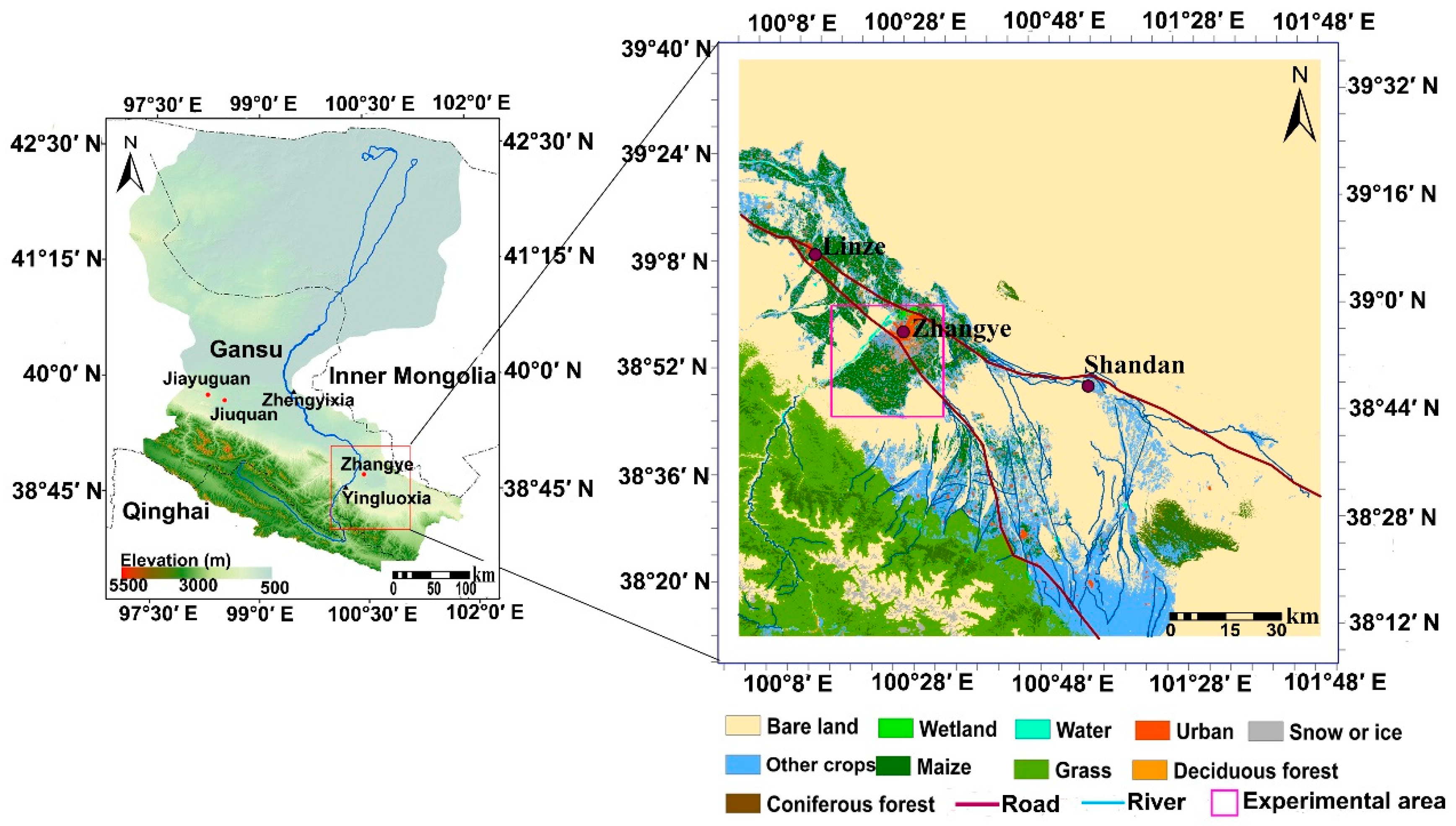
A case study was conducted in the areas near the middle of the Heihe River watershed in an arid and semi-arid area in North-western China (38°10′N~39°35′N and 99°57′E~101°46′E), and the location of the study area and land-use types are shown in Figure 1. Land-use types in the study area mainly include croplands, bare land, wetland, forest and grass. Crop lands are mainly distributed throughout the oasis of Zhangye in western areas, and the Gobi Desert constitutes the dominant land use types in the north-eastern areas. The topography of this area varies significantly from northeast to southwest, and can be divided into plains and mountains with elevations ranges from 1200 m to 5000 m. Bare lands are mainly located in the north-east, while the mountains are mainly distributed in the southwestern areas. This area has a temperate continental climate, with an average annual air temperature of about 6 °C~8 °C, an average annual precipitation about 100 mm~250 mm and an average annual pan evaporation about 1200 mm~1800 mm. Influenced by Asian monsoon, most rainfall occurs from May to September in the rainy season, and decreases from south to north. Maize is the main crop of the agricultural land in the oasis, and they are irrigated about once a month by canal irrigation.
2.2. Data and Data Processing
2.2.1. Remote Sensing Data
MODIS LAI/FPAR products. The MODIS LAI/FPAR products (MOD15 C55) [31] with a spatial resolution of 1 km were provided on an 8-day basis. The LAI/FPAR retrieve algorithm consisted of a main procedure that exploits the spectral information content of MODIS surface reflectance at up to seven spectral bands and a backup algorithm that uses empirical relationships between Normalized Difference Vegetation Index (NDVI) and canopy LAI and FPAR [32]. The main algorithm employed a biome-dependent look-up table approach based on simulations with a stochastic radiative transfer model that considered three-dimensional canopy structure [32]. The back-up algorithm was triggered to estimate the LAI and FPAR using vegetation indices when this main algorithm failed. The validation methods include comparisons with in situ data, comparisons with data from airborne and other space borne sensors, analysis of trends in products [32]. In this study, MODIS LAI/FPAR products from June to September 2012 in the study area were used to generate high resolution LAI and FPAR from the downscaling method.
GLASS LAI/FPAR products. GLASS LAI/FPAR products from June to September 2012 in study area were also used to generate high resolution LAI and FPAR from the downscaling method. The GLASS LAI/FPAR products were generated and released by the Center for Global Change Data Processing and Analysis of Beijing Normal University [33], and are also available from the Global Land Cover Facility [34]. The temporal resolution of the products is 8 days and spatial resolution is 1 km. The GLASS LAI product was generated from time-series MODIS and AVHRR reflectance data using general regression neural networks, and was believed to be more temporally continuous and spatially complete than the MODIS LAI product [35]. Furthermore, the GLASS FPAR product was generated from the GLASS LAI product, thus, showed the same properties as the GLASS LAI product.
Landsat data. Landsat-7 Enhanced Thematic Mapper Plus (ETM+) images [36] in 10 July 2012 were used to derive high resolution LAI and FPAR from a regression tree approach in this study. The data were first destriped, and then surface reflectance was obtained after radiometric correction and atmospheric correction. Then a regression tree [37] was then established between a reference dataset (MODIS LAI and FPAR/GLASS LAI and FPAR) and pixel-aggregated Landsat surface reflectance, and then applied to Landsat imagery to estimate LAI and FPAR at 30 m resolution.
Landcover data. GlobeLand30 landcover map, which was comprised of ten landcover types, including forests, artificial surfaces and wetlands, was used in this paper [38,39]. This map was extracted from more than 20,000 Landsat and Chinese HJ-1 satellite images. The spatial resolution of the landcover map was 30 m.
2.2.2. Meteorological Data
Meteorological data, including the daily maximum temperature, the daily minimum temperature and the daily mean temperature, were firstly collected from meteorological stations in the study area, and were interpolated to 30 m by using the method of Kriging interpolation. Then eight day mean temperature was obtained by averaging the daily values. Daily solar shortwave radiation with a resolution of 30 m was obtained through a Mountain Microclimate Simulation Model (MT-CLIM) [40], and then eight day mean solar shortwave radiation were obtained by averaging the daily values.
2.2.3. Field Data
Ground-based field carbon flux data used in this study were derived from the MUlti-Scale Observation EXperiment on Evapotranspiration over heterogeneous land surfaces 2012 of the Heihe Watershed Allied Telemetry Experiment Research (HiWATER-MUSOEXE) [41,42,43]. A 30 km × 30 km experimental region was set up according to landscape situations, agricultural structures and irrigation status in the study area, in which distributed 21 field observation sites. A core experimental area consists of 17 field observation sites distributed in a 5.5 km × 5.5 km region. All the observation sites were distributed in the middle of the study area, as shown in Figure 2 [44]. Land use types of the 21 field observation sites, including croplands (mainly maize), orchard, vegetable field, desert, desert steppe, Gobi and wetland. The eddy covariance systems and meteorological tower were set in each observation site. Half-hourly data of carbon flux were obtained from the eddy covariance systems, and meteorological variables were obtained from the meteorological tower. Gap-filling and flux-partitioning were processed using the Edire software package. Then daily carbon flux was obtained by averaging the half-hourly data. Daily ground-based GPP were obtained by partitioning the observed net flux into GPP and ecosystem respiration according to Coops et al. [45], Wang et al. [46], and Zhang et al. [47] from 9 June to 16 September 2012 from the 21 field observation sites; then, eight days mean GPP were calculated by averaging the daily GPP. The ground based eight days GPP from 21 observation sites were used to direct validate the GPP estimates in our study.
2.3. Methods
To generate time series high resolution GPP/NPP, a LUE model based on the downscaling method was adopted in this paper, as shown in Figure 3. First, high resolution (30 m) FPAR and LAI were obtained by using the downscaling method, and high resolution (30 m) temperature and water stress were obtained through interpolation. Second, time series high resolution GPP and NPP were estimated from a LUE GPP/NPP model. To assess the performance of the method, the GPP and NPP estimates were validated with the ground-based field data, and were compared with the MODIS and GLASS vegetation productivity products.
2.3.1. Downscaling of FPAR and LAI
The Spatio-Temporal Enhancement Method for medium resolution LAI (STEM-LAI) [25] was adopted to downscale 1 km MODIS LAI/GLASS LAI to 30 m LAI. The STEM-LAI is a downscaling method based on STARFM and regression tree to generate time series high resolution LAI from MODIS data and Landsat images. As STARFM is extendable to some other biophysical properties [1,25], such as evaporation [23] and land surface temperature [24], high resolution FPAR data were also derived from this method. The specific steps of LAI and FPAR downscaling as follows:
Firstly, high-quality MODIS/GLASS LAI samples retrieved from the main algorithm were selected based on the product quality flags. The MODIS/GLASS LAI product provide quality control flags for each pixel. The quality control flags embedded in the MODIS and GLASS product reflect the retrieval quality reasonably well. To ensure that only the best quality of data are being used in the regression tree training.
Then the homogeneous MODIS/GLASS pixels were selected by using the coefficients of variation of the Landsat pixels inside each MODIS/GLASS 1 km pixel. The coefficient of variation was defined as the ratio of the standard deviation to the mean value [37]. The coefficient of variation (CV) was computed and averaged among all Landsat spectral bands from Landsat surface reflectance inside each MODIS/GLASS pixel cell [37]. The CV described the relative variation of a MODIS/GLASS pixel in a Landsat resolution (30 m). The smaller the CV was, the purer the MODIS/GLASS pixel was. If the band averaged CV of a MODIS/GLASS pixel was less than a threshold, the MODIS/GLASS pixel was considered to be a homogeneous sample.
A regression tree approach [37] was then established between a reference dataset (MODIS LAI/GLASS LAI) and pixel-aggregated Landsat surface reflectance, and then applied to Landsat imagery to estimate LAI at 30 m resolution during the Landsat acquisition dates. Specifically, high quality MODIS LAI/GLASS LAI retrievals from homogeneous pixels were used as reference samples to build rule-based Cubist regression tree [48] that relate low resolution LAI samples to aggregated Landsat surface reflectance via multivariate linear regression, then the high resolution LAI (30 m) on the Landsat acquisition data could be obtained from the regression tree. The cubist regression tree method was a data mining approach that builds rule-based predictive multivariate linear regression models based on available samples.
At last, STARFM was then applied to time series MODIS LAI/GLASS LAI (1 km) and Landsat derived high resolution LAI (30 m) data streams to interpolate high spatial resolution LAI. As STARFM is extendable to some other biophysical properties [1,25] so long as the multi-scale input data streams are comparable and spatially and temporally consistent, high resolution FPAR data were also derived from this method.
2.3.2. Estimation of GPP and NPP
To estimate high resolution GPP and NPP by integrating remote sensing data and eco-physiological processes, the Multi-source data Synergized Quantitative (MusyQ) GPP/NPP algorithm [5,44] was adopted in this paper. The MusyQ GPP/NPP algorithm is essentially a LUE model. GPP could be described as [49]:
where PAR is the photosynthetically active radiation (PAR), and is the biome-specific potential LUE, which could be obtained through a biome-specific potential Look-Up Table (LUT) by referring to land cover categories of the Biome Properties Look-Up Table (BPLUT) of the MODIS GPP/NPP algorithm [50], shown in Table 1.
and are the down-regulation effects of temperature and water conditions on , respectively. could be calculated according to the Carnegie, Ames, Stanford Approach (CASA) [51]. was calculated by [52]:
where NDWI is the normalized difference water index, is the maximum NDWI in the growing season, and and are the reflectance in near-infrared band and mid- infrared band, respectively.
NPP is the net flow of carbon from the atmosphere to plants, which is defined as the balance between GPP and autotrophic respiration [5,44,51].
where is autotrophic respiration. Ra could be separated into two parts, maintenance respiration , which refers to the energy necessary to maintain biomass, and growth respiration which refers to the energy needed for converting assimilates into new structural plant constituents [5,44].
were estimated separately for non-forest and forest lands. For non-forest land, was estimated with LAI and specific leaf area (SLA) [5,44].
where SLA was obtained from the BPLUT of MODIS GPP/NPP algorithm [50] in our model.
For forest land, was defined as the summation of the maintenance respiration of leaves, stems, and roots [5,44].
where is the biomass of plant component i, is maintenance respiration coefficient for component i, is the temperature sensitivity factor, T is the daily average temperature and is the base temperature, is the maintenance respiration coefficient. Forest lands are classified as four classes, needle-leaf forests, broadleaved forests, mixed forests and others, and and for each classes are obtained according to the BPLUT of MODIS GPP/NPP algorithm [50]. Specifically, leaf mass is estimated from LAI and SLA [5,44]:
2.3.3. Accuracy Assessment
To assess the performance of downscaling method proposed in this paper, the estimated GPP from the MusyQ GPP algorithm was validated with the ground observed GPP. Noting that the mean GPP values in a 3 pixels 3 pixels window around each observation site were used to compare with the ground observed GPP to decrease the co-registration errors between images and observation sites. Besides, the estimated GPP and NPP were validated with high resolution GPP and NPP pixel by pixel. The Determination Coefficient (R2), Root Mean Square Error (RMSE) and Mean Relative Error (MRE) were used to quantify the downscaled GPP and NPP.
3. Results
3.1. Validation of Downscaled FPAR and LAI
3.1.1. Cross Validation of Downscaled FPAR and LAI
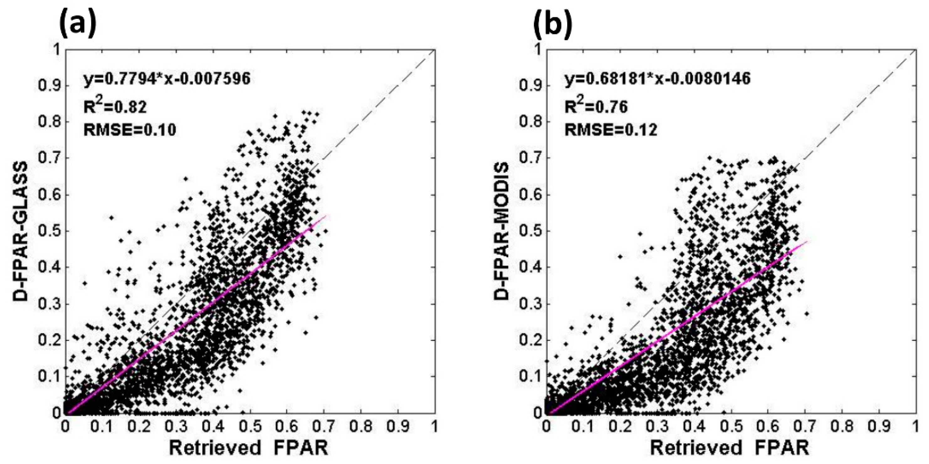
The downscaled 30 m FPAR and LAI demonstrate finer scale features with a clear identification and have a high accuracy (Figure 4 and Figure 5). We compared the downscaled FPAR/LAI in July 2012 with corresponding retrieved high resolution (30 m) FPAR/LAI products by [54]. Specifically, the high resolution (30 m) LAI and FPAR was retrieved by using an instantaneous quantitative model based on the law of energy conservation and the concept of recollision probability [5] from Chinese HJ-1B satellite observations data. This model separated direct energy absorption in the canopy from energy absorption caused by multiple scattering between the soil and the canopy, and took the direct sunlight and diffuse skylight into consideration. Validation against field measurements indicated that FPAR and LAI retrievals had high accuracy [54]. In general, a good linear relationship existed between the downscaled FPAR and retrieved FPAR (Figure 6), R2 could reach 0.82 and 0.76 of the downscaled FPAR from GLASS data (D_FPAR_GLASS) and downscaled FPAR from MODIS data (D_FPAR_MODIS), respectively. RMSE between downscaled FPAR and retrieved FPAR were 0.10 and 0.12 respectively. Meanwhile, good consistency was shown between the downscaled LAI and retrieved LAI (Figure 7). RMSE between the downscaled LAI and retrieved LAI were 0.63 and 0.69, respectively. However, we found that most plots in Figure 6 were distributed under the 1:1 line, which demonstrated that both the downscaled LAI from GLASS data (D_LAI_GLASS) and the downscaled LAI from MODIS data (D_LAI_MODIS) were lower than the retrieved LAI from the HJ-1B data. The main reason may be that the problem of mixed pixels led to the low values of the reference data, i.e., GLASS and MODIS 1 km LAI. Specifically, some other types of land cover (such as bare land, grassland and artificial land) exist in a GLASS/MODIS 1 km pixel, which may lead to low values of LAI in the growing season. Furthermore, high resolution (30 m) FPAR/LAI products from HJ-1 were generated monthly and retrieved from the maximum value in the month, which could also have led to the overestimation of FPAR and LAI.
3.1.2. Comparison of FPAR and LAI Time Series
Temporal dynamic patterns of the downscaled FPAR, GLASS FPAR and MODIS FPAR from 17 field observation sites, which were mainly covered by vegetation are shown in Figure 8. In general, the time series of the D_FPAR_GLASS, D_FPAR_MODIS, MODIS FPAR and GLASS FPAR agreed well in cropland, orchard, vegetable field and wetland. It could be clearly seen that GLASS FPAR was more continuous with smoother trajectories, therefore, D_FPAR_GLASS showed the same properties as GLASS FPAR, i.e., the time series was also continuous. FPAR time series increased initially then decreased after reaching the peak around July (DOY 185–216). In cropland, the D_FPAR_GLASS, D_FPAR_MODIS, MODIS FPAR and GLASS FPAR agreed better in August and September (DOY 217–280), but the GLASS FPAR was about 0.1~0.2 lower than the MODIS FPAR and downscaled FPAR in June, July and August. The MODIS FPAR could be as high as about 0.8 while the GLASS FPAR was only about 0.6 in the peak of growing season. MODIS FPAR was the highest in the whole growing season in vegetable land, as shown in Figure 7c, except for a low value that appeared in July (DOY 201–208), which led to a low value in the D_FPAR_MODIS. Time series of the GLASS FPAR and D_FPAR_GLASS in vegetable land were obviously more continuous. In orchard and wetland, we could find that good agreements were generally achieved among D_FPAR_GLASS data, D_FPAR_MODIS, MODIS FPAR and GLASS FPAR generally. But in orchard, the MODIS FPAR was higher than the others in the early growing season.
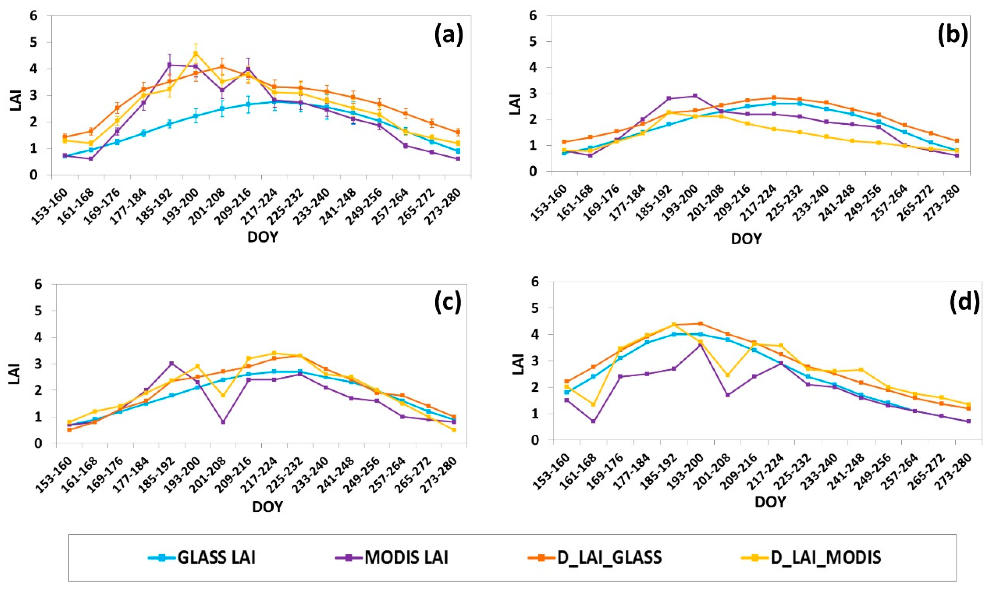
Generally, D_LAI_GLASS, D_LAI_MODIS, MODIS LAI and GLASS LAI agreed well in most times (Figure 9). We also found that time series of GLASS LAI and D_LAI_GLASS were more continuous with smoother trajectories. In cropland, GLASS LAI was less than 3 in June and July, which was lower than the MODIS LAI and the downscaled LAI. MODIS LAI and D_LAI_MODIS were a little lower than the GLASS LAI and D_LAI_GLASS in August and September in orchard. In the vegetable field, downscaled LAI, GLASS LAI and MODIS LAI achieved good agreements, but GLASS LAI was more continuous. In wetland, MODIS LAI was less than 3 in June and July, which was lower than the downscaled LAI and GLASS LAI.
3.2. Validation of Estimated GPP and NPP
3.2.1. Validation Against Ground-Based GPP
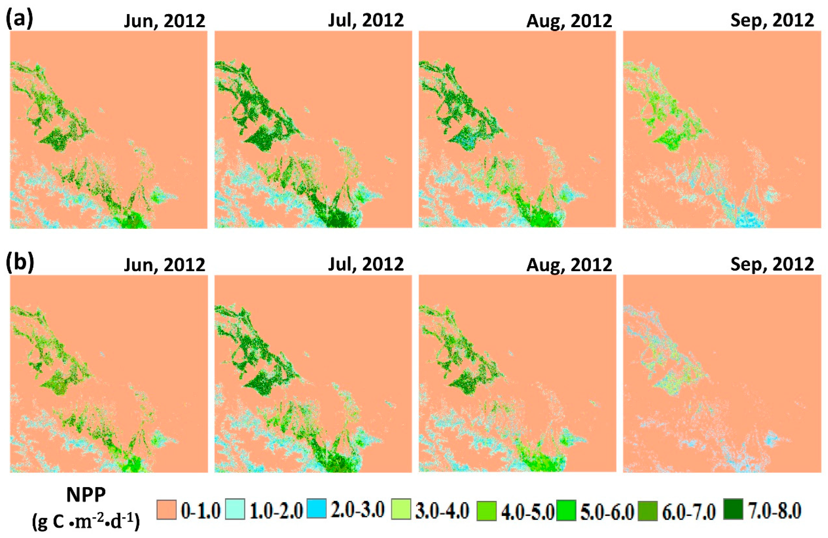
Spatial distribution of high resolution (30 m) GPP (Figure 10) and NPP (Figure 11) were obtained according to the method proposed in Section 2.3. We found the GPP and NPP reached their maximum in July and August. Areas covered with crops occupied the highest values of GPP and NPP, followed by the mountainous areas. Regions covered with deserts and Gobi demonstrated the lowest GPP and NPP values. Validation against the ground measurements demonstrated that both the GPP base on downscaled GLASS data (D_GPP_GLASS) and GPP based on downscaled MODIS data (D_GPP_MODIS), had high accuracy. In general, a good linear relationship existed between the downscaled GPP and ground-based GPP. R2 between the ground-based GPP and D_GPP_GLASS could be as high as 0.78, and the RMSE was 2.69 g Cm−2d−1 (Figure 12a). The R2 between the ground-based GPP and D_GPP_MODIS could be as high as 0.84, and the RMSE is 2.20 g Cm−2d−1 (Figure 12b). Mean relative error (MRE) of D_GPP_GLASS was 5.07%, and MRE of D_GPP_MODIS was 3.21%.
We compared the precision of the high resolution (30 m) D_GPP_GLASS, D_GPP_MODIS, with the low resolution (1 km) MODIS GPP (MOD17 C55) and the estimated GLASS GPP (Figure 12c,d). MOD17 products were an application of the described radiation conversion efficiency concept to predictions of daily GPP using a LUE model based on the MOD12 land cover product, Data Assimilation Office (DAO) meteorological datasets, and the MOD15 LAI/FPAR products [55]. The estimated GLASS GPP and NPP products with a spatial resolution of 1km and temporal resolution of the 8-day were generated by the GLASS FPAR and LAI data from the MusyQ GPP/NPP algorithm [5]. We could find that estimated GLASS GPP and MODIS GPP underestimate ground-based GPP in most vegetation types. RMSE between estimated GLASS GPP and ground-based GPP could be as high as 6.42 g Cm−2d−1, while the RMSE between estimated MODIS GPP and ground-based GPP could reach 7.09 g Cm−2d−1. A higher R2 and lower RMSE demonstrated that the GPP from the downscaled data achieved a better precision than the low resolution (1 km) estimated GLASS GPP and MODIS GPP, and indicated the applicability and reliability of the method proposed in this paper in generating high resolution GPP.
3.2.2. Cross Validation Against High Resolution GPP and NPP
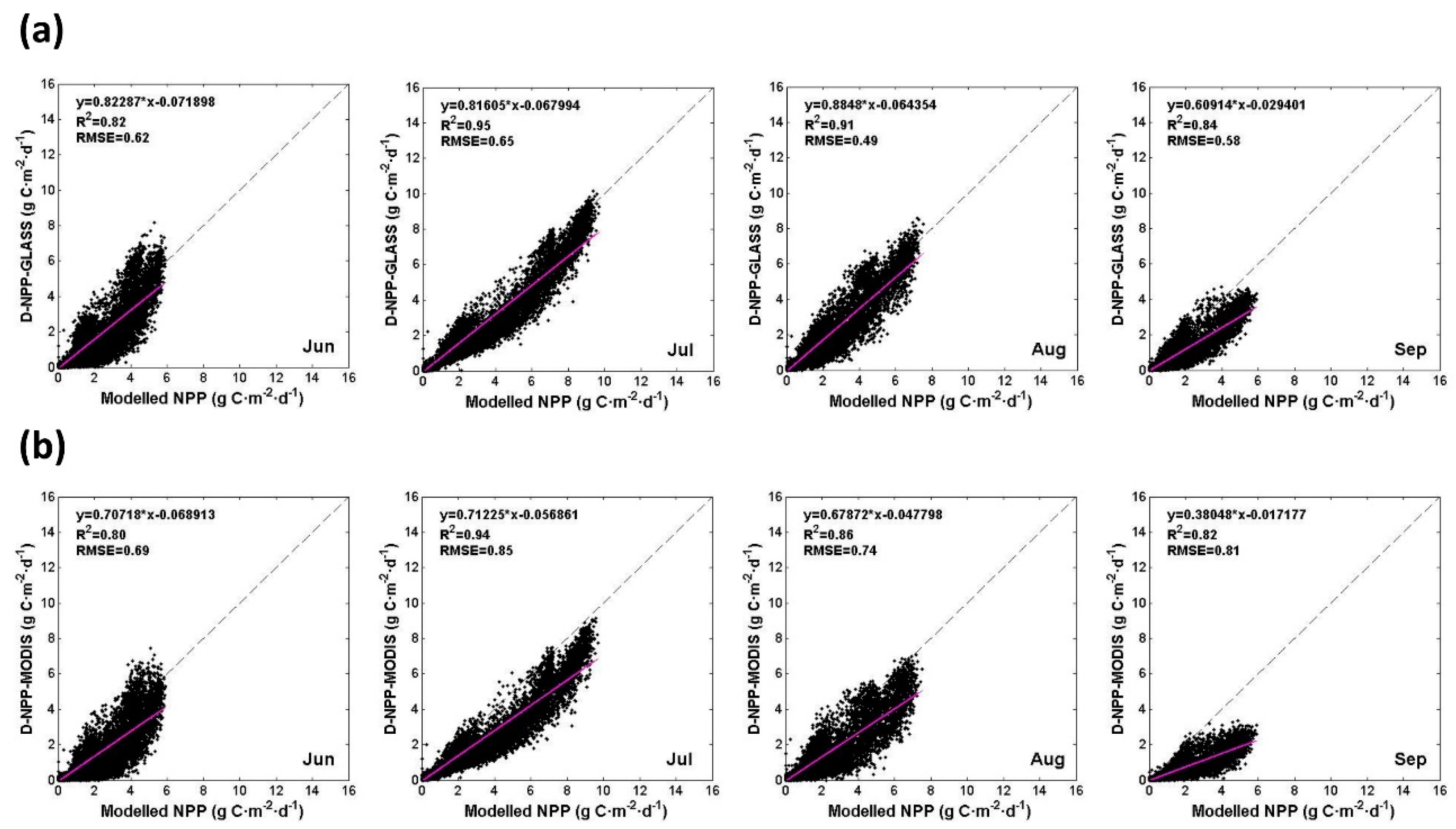
We compared the downscaled GPP/NPP with the high resolution GPP/NPP, which was derived from high resolution FPAR and LAI data by using the MusyQ GPP/NPP algorithm. Specifically, the high resolution (30 m) LAI and FPAR were retrieved by using an instantaneous quantitative model based on the law of energy conservation and the concept of recollision probability from Chinese HJ-1B satellite observations data [54]. Figure 13 demonstrated the comparison of the downscaled GPP against high resolution GPP. In general, a good linear relationship existed between the downscaled GPP and modelled GPP. R2 was greater than 0.8, and RMSE was less than 1.5 g Cm−2d−1 from June to September. But, we could found that both D_GPP_GLASS and D_GPP_MODIS somewhat underestimated modelled GPP in most times. As for the NPP estimates, as shown in Figure 14, the estimated NPP showed good consistency with the modelled NPP. NPP from downscaled GLASS data (D_NPP_GLASS) and NPP from downscaled MODIS data (D_NPP_MODIS) underestimated modelled NPP in September.
3.3. Comparison of GPP and NPP Time Series
Among the twenty field measurement sites, we chose seventeen sites that were mainly covered by vegetation to analyze the temporal dynamic patterns of GPP and NPP during the growing season of 2012. These 17 sites included 14 sites in croplands, one in orchard, one in vegetable field and one in wetland. The time series of the ground-based GPP, MODIS GPP, estimated GLASS GPP, D_GPP_MODIS and D_GPP_GLASS were shown in Figure 15. In cropland, we could find that D_GPP_MODIS and D_GPP_GLASS agreed better with the ground-based GPP in most times. While the MODIS GPP and estimated GLASS GPP underestimated the ground measurement GPP significantly, and could not reflect the temporal patterns of GPP. The MODIS GPP and estimated GLASS GPP were less than 6 g Cm−2d−1 during the whole growing season, but the GPP D_GPP_GLASS and D_GPP_MODIS were higher than 8 g Cm−2d−1 in most times, and could be as high as 16 g Cm−2d−1 at the peak of growing season. In orchard, estimated GLASS GPP and MODIS GPP were about 3~4 g Cm−2d−1 lower than ground-based GPP, GPP D_GPP_GLASS and D_GPP_MODIS. But estimated GLASS GPP and MODIS GPP achieved good agreements. In vegetable field, the time series of the ground-based GPP, MODIS GPP, estimated GLASS GPP, D_GPP_GLASS and D_GPP_MODIS matched well in most times. In wetland, MODIS GPP underestimated the ground based GPP obviously, while estimated GLASS GPP matched well with ground-based GPP, D_GPP_GLASS and D_GPP_MODIS.
Temporal patterns of the estimated GLASS NPP, D_NPP_MODIS and D_NPP_GLASS were demonstrated in Figure 16. In cropland, the temporal variation trend of D_NPP_MODIS and D_NPP_GLASS matched well. But estimated GLASS NPP was lower than 4 g Cm−2d−1 in the growing season, which was much lower than D_NPP_MODIS and D_NPP_GLASS. In orchard, vegetable field and wetland, estimated GLASS NPP, D_NPP_MODIS and D_NPP_GLASS generally achieved good agreements generally. In vegetable field and wetland, estimated GLASS NPP is a little higher than D_NPP_MODIS and D_NPP_GLASS.
4. Discussion
4.1. Comparison of the Accuracy of GPP Estimates from STARFM
In this paper, a framework to generate high resolution GPP and NPP dataset at 30 m was developed based on downscaling method from Landsat data and MODIS/GLASS data. Direct validation against ground measurement data and cross validation against high resolution images demonstrated that this downscaling framework could obtain time series high temporal and spatial resolution GPP and NPP datasets. Data fusion approaches have been demonstrated to be feasible and efficient ways to synthesize time series images from multi-scale remote sensing data at different spatial and temporal resolutions [26,55,56]. The STARFM has been found to be applicatable to produce an accurate interpolated NDVI time series in many studies [55,57]. Furthermore, based on the time series high resoltution NDVI generated from STARFM, and the liner relationship between FPAR and NDVI, some studies have been carried out to estimate GPP and NPP from the LUE model [26,30,58]. However, the relationship between MODIS and Landsat NDVI may vary, due to different acquisition dates and cloud contamination, aerosols, viewing angles and temporal compositing [58], and the relation between FPAR and NDVI also changes with vegetation type and solar zenith angle [59], all these factors can introduce uncertainties into the FPAR estimation and GPP/NPP estimation. In our study, time series FPAR were generated from MODIS/GLASS FPAR products, which have been temporal infilled of cloud-contaminated pixels, and have been validated to be in good quality with high accuracy. Owing to the lack of ground observations, the downscaled GPP were validated with MODIS GPP product at 1 km scale (R2 ranged from 0.55 to 0.81, and RMSE ranged from 1.39 g Cm−2d−1 to 3.92 g Cm−2d−1) [20,21] or validated with Landsat derived GPP (R2 ranged from 0.85 to 0.86) in previous studies (Table 2) [26]. In this study, the downscaled GPP were validated with both high resolution GPP at 30 m scale (R2 ranged from 0.81 to 0.95, and RMSE ranged from 0.84 g Cm−2d−1 to 1.55 g Cm−2d−1) and ground observed data (R2 ranged from 0.71 to 0.90, and RMSE ranged from 0.87 g Cm−2d−1 to 3.14 g Cm−2d−1). The validation results demonstrated that both the GPP from downscaled GLASS data and from MODIS data had higher accuracy.
4.2. Uncertainties Analysis
The errors of the input data of the downscaling process would have influence on the accuracy of the downscaling results. Although both GLASS LAI/FPAR products (RMSE = 0.7848 and R2 = 0.8095 for the LAI product, R2 = 0.9292 and RMSE =0.0716 for the FPAR product) [6,7] and MODIS LAI/FPAR products (RMSE = 1.1173 and R2 = 0.6705 for the LAI product, R2 = 0.8048 and RMSE = 0.1276 for the FPAR product) [3,4] have high accuracy, the errors of the GLASS and MODIS product certainly have some impact on the accuracy of downscaling FPAR and LAI, and then have some influence in the GPP and NPP estimates. Second, there are stripes in the original Landsat ETM+ images, the destripe process may introduce errors in the high spatial resolution surface reflectance data, which will bring additional errors to the final high spatial and temporal LAI/FPAR products.
The process of FPAR and LAI downscaling would also bring some uncertainties in estimating high resolution GPP and NPP. In our study, the high spatial resolution of FPAR and LAI were retrieved by Cubist regression tree approach from Landsat ETM+ data using MODIS/GLASS FPAR and LAI products as a reference. Although the Cubist regression tree have the ability to predict outside the range of values in the training dataset, the accuracy of the regression tree approach still relied on the data quality and distribution of training dataset [37]. If high quality data are limited, the regression tree approach may not be stable for FPAR and LAI retrievals. Because of large heterogeneity of land surface in the study area, most of GLASS/MODIS 1 km pixels are mixed pixels, the low fraction of vegetation cover land cover types (such as bare land, grassland and artificial land) existed in a mixed GLASS/MODIS 1 km pixel will lead to the low values of the reference data, i.e., GLASS/MODIS 1 km FPAR and LAI, in the growing season [60,61]. Therefore, the FPAR and LAI estimates from the regression tree approach may not be able to describe the high values of FPAR and LAI, as shown in Figure 6 and Figure 7.
The precision of reference high spatial resolution data and the spatial representativeness of ground observation data are also related to the performance assessment of the downscaling method. In this paper, high resolution (30 m) FPAR/LAI retrievals based on the law of energy conservation and the concept of recollision probability were used to validate the downscaled FPAR and LAI. Some errors exist in geometric correction when retrieving the FPAR and LAI from the Chinese HJ-1B satellite data, which could lead to some uncertainty in the downscaled FPAR and LAI validation. Moreover, satellite pixel scale and the footprint size of ground observation may be another factor that influenced the accuracy when validating the GPP estimates. The spatial representativeness of the observed GPP data related to the height of the eddy covariance instruments. In this study, the heights of the eddy covariance instruments range from 2.85 m to 4.50 m, the footprint size of carbon flux is mainly smaller than 200 m, and the spatial representative of ground observation is more close to the 30 m scale, which is the reason why the accuracy of downscaled GPP is higher. The large number of carbon flux station in the maize cropland, small footprint size of ground observed GPP data, and mixed pixel phenomenon are the main reasons of GPP underestimation at 1 km scale compared with ground observed data.
4.3. Future Work
Bias of the downscaled FPAR and LAI in our study, may have introduced some considerable errors in the GPP and NPP estimation. Specifically, FPAR is related to the absorbed radiation in GPP estimation and LAI was related to the maintenance respiration in NPP estimation. In the future, we may carry out research into the error transfers in GPP and NPP estimates when using the downscaled FPAR and LAI in the MuSyQ GPP/NPP algorithm. Second, the STARFM predictions were affected by the number of spectral slices, the maximum search distance and the method used to inform the search for similar neighbor pixels [1,25]. Therefore, we may do some further analysis on the parameter optimization in the GPP and NPP predictions. Third, STARFM did not gain the ability to accurately predict short-term, transient changes that are not recorded in any of the bracketing fine-resolution images, therefore combining STARFM with ESTARFM and STAARCH may be a feasible way to solve the problem in generating high resolution vegetation productivity [21]. To improve the accuracy of the downscaling results, higher quality low resolution data would be used, and some improvements model of STARFM would be adopted. Improving the method to match the scale between ground observation data and satellite derived data, would be another way to improve the accuracy of downscaling results.
5. Conclusions
Downscaling methods in remote sensing provide a new observational approach to estimate high resolution vegetation productivity. In this paper, a method to generate high spatial resolution (30 m) GPP and NPP products based on low resolution (1000 m) FPAR and LAI data was developed. First, the time series of downscaled high resolution FPAR and LAI were obtained on the basis of STARFM and a regression tree approach. Then high resolution GPP and NPP were estimated by using the MuSyQ GPP/NPP algorithm. At last, downscaled GPP and NPP were validated by using ground-based data and high resolution data. The results of this paper indicated the applicability and reliability of the downscaling method in generating high resolution time series GPP and NPP.
Generally, good consistency existed between the downscaled FPAR/LAI and inverted FPAR/LAI. The time series of D_FPAR_GLASS, D_FPAR_MODIS, MODIS FPAR and GLASS FPAR agreed well in cropland, orchard, vegetable field and wetland. Second, direct validation against the ground-based data and cross validation against the high resolution data showed that downscaled GPP achieved high accuracy. GPP from the downscaled data achieved a better precision than the estimated GLASS GPP and MODIS GPP. R2 between the D_GPP_GLASS and ground-based GPP could be as high as 0.78, and RMSE was only 2.69 g Cm−2d−1 And R2 between D_GPP_MODIS and ground-based GPP could reach 0.84, and RMSE was only 2.20 g Cm−2d−1. Third, the ground-based GPP, MODIS GPP, estimated GLASS GPP, D_GPP_MODIS and D_GPP_GLASS achieved good agreements. Temporal patterns of estimated GLASS NPP, D_NPP_MODIS and D_NPP_GLASS were also generally consistent. But estimated GLASS NPP in cropland was also relatively lower than D_NPP_MODIS and D_NPP_GLASS.
Author Contributions
T.Y. and R.S. proposed the ideas; T.Y., Z.X., Q.Z., J.W. and G.L. preprocessed and analyzed the data; T.Y. and R.S. prepared the paper.
Funding
This research was funded by the National Key R&D Program of China, grant number 2016YFB0501502, and the National Natural Science Foundation of China, grant number 41471349, 41531174 and 61661136006001.
Acknowledgments
This work was supported by the National Key R&D Program of China (2016YFB0501502), the National Natural Science Foundation of China (41471349, 41531174 and 61661136006001).
Conflicts of Interest
The authors declare no conflict of interest.
References
- Gao, F.; Masek, J.; Schwaller, M.; Hall, F. On the blending of the Landsat and MODIS surface reflectance: Predicting daily Landsat surface reflectance. IEEE Trans. Geosci. Remote Sens. 2006, 44, 2207–2218. [Google Scholar] [CrossRef]
- Gevaert, C.M.; García-Haro, F.J. A comparison of STARFM and an unmixing-based algorithm for Landsat and MODIS data fusion. Remote Sens. Environ. 2015, 156, 34–44. [Google Scholar] [CrossRef]
- Running, S.W.; Nemani, R.R.; Heinsch, F.A.; Zhao, M.; Reeves, M.; Hashimoto, H. A continuous satellite-derived measure of global terrestrial primary production. AIBS Bull. 2004, 54, 547–560. [Google Scholar] [CrossRef]
- Heinsch, F.A.; Reeves, M.; Bowker, C.F. User’s Guide, GPP and NPP (MOD 17A2/A3) Products, NASA MODIS Land Algorithm. Available online: https://www.researchgate.net/publication/242118371_User’s_guide_GPP_and_NPP_MOD17A2A3_products_NASA_MODIS_land_algorithm (accessed on 5 October 2018).
- Yu, T.; Sun, R.; Xiao, Z.; Zhang, Q.; Liu, G.; Cui, T.; Wang, J. Estimation of Global Vegetation Productivity from Global LAnd Surface Satellite Data. Remote Sens. 2018, 10, 327. [Google Scholar] [CrossRef]
- Xiao, Z.; Liang, S.; Sun, R.; Wang, J.; Jiang, B. Estimating the fraction of absorbed photosynthetically active radiation from the MODIS data based GLASS leaf area index product. Remote Sens. Environ. 2015, 171, 105–117. [Google Scholar] [CrossRef]
- Xiao, Z.; Liang, S.; Wang, J.; Xiang, Y.; Zhao, X.; Song, J. Long-time-series global land surface satellite leaf area index product derived from MODIS and AVHRR surface reflectance. IEEE Trans. Geosci. Remote Sens. 2016, 54, 5301–5318. [Google Scholar] [CrossRef]
- Atkinson, P.M. Downscaling in remote sensing. Int. J. Appl. Earth Obs. 2013, 22, 106–114. [Google Scholar] [CrossRef]
- Carper, W.; Lillesand, T.; Kiefer, R. The use of intensity-hue-saturation transformations for merging SPOT panchromatic and multispectral image data. Photogramm. Eng. Remote Sens. 1990, 56, 459–467. [Google Scholar]
- Shettigara, V.K. A generalized component substitution technique for spatial enhancement of multispectral images using a higher resolution data set. Photogramm. Eng. Remote Sens. 1992, 58, 561–567. [Google Scholar]
- Yocky, D.A. Multiresolution wavelet decomposition I me merger of landsat thematic mapper and SPOT panchromatic data. Photogramm. Eng. Remote Sens. 1996, 62, 1067–1074. [Google Scholar]
- Acerbi-Junior, F.W.; Clevers, J.G.P.W.; Schaepman, M.E. The assessment of multi-sensor image fusion using wavelet transforms for mapping the Brazilian Savanna. Int. J. Appl. Earth Obs. 2006, 8, 278–288. [Google Scholar] [CrossRef]
- Zhang, Y. Understanding image fusion. Photogramm. Eng. Remote Sens. 2004, 70, 657–661. [Google Scholar]
- Stathopoulou, M.; Cartalis, C. Downscaling AVHRR land surface temperatures for improved surface urban heat island intensity estimation. Remote Sens. Environ. 2009, 113, 2592–2605. [Google Scholar] [CrossRef]
- Pouteau, R.; Rambal, S.; Ratte, J.P.; Gogé, F.; Joffre, R.; Winkel, T. Downscaling MODIS-derived maps using GIS and boosted regression trees: The case of frost occurrence over the arid Andean highlands of Bolivia. Remote Sens. Environ. 2011, 115, 117–129. [Google Scholar] [CrossRef]
- Yang, F.; White, M.A.; Michaelis, A.R.; Ichii, K.; Hashimoto, H.; Votava, P.; Zhu, A.-X.; Nemani, R.R. Prediction of continental-scale evapotranspiration by combining MODIS and AmeriFlux data through support vector machine. IEEE Trans. Geosci. Remote Sens. 2006, 44, 3452–3461. [Google Scholar] [CrossRef]
- Kaheil, Y.H.; Rosero, E.; Gill, M.K.; McKee, M.; Bastidas, L.A. Downscaling and forecasting of evapotranspiration using a synthetic model of wavelets and support vector machines. IEEE Trans. Geosci. Remote Sens. 2008, 46, 2692–2707. [Google Scholar] [CrossRef]
- Han, D.; Kwong, T.; Li, S. Uncertainties in real-time flood forecasting with neural networks. Hydrol. Process. 2007, 21, 223–228. [Google Scholar] [CrossRef]
- Tatem, A.J.; Lewis, H.G.; Atkinson, P.M.; Nixon, M.S. Super-resolution target identification from remotely sensed images using a Hopfield neural network. IEEE Trans. Geosci. Remote Sens. 2001, 39, 781–796. [Google Scholar] [CrossRef] [Green Version]
- Hilker, T.; Wulder, M.A.; Coops, N.C.; Linke, J.; McDermid, G.; Masek, J.G.; Gao, F.; White, J.C. A new data fusion model for high spatial-and temporal-resolution mapping of forest disturbance based on Landsat and MODIS. Remote Sens. Environ. 2009, 113, 1613–1627. [Google Scholar] [CrossRef]
- Zhu, X.; Chen, J.; Gao, F.; Chen, X.; Masek, J.G. An enhanced spatial and temporal adaptive reflectance fusion model for complex heterogeneous regions. Remote Sens. Environ. 2010, 114, 2610–2623. [Google Scholar] [CrossRef]
- Xie, D.; Zhang, J.; Zhu, X.; Pan, Y.; Liu, H.; Yuan, Z.; Yun, Y. An improved STARFM with help of an unmixing-based method to generate high spatial and temporal resolution remote sensing data in complex heterogeneous regions. Sensors 2016, 16, 207. [Google Scholar] [CrossRef] [PubMed]
- Cammalleri, C.; Anderson, M.C.; Gao, F.; Hain, C.R.; Kustas, W.P. Mapping daily evapotranspiration at field scales over rainfed and irrigated agricultural areas using remote sensing data fusion. Agric. For. Meteorol. 2014, 186, 1–11. [Google Scholar] [CrossRef]
- Weng, Q.; Fu, P.; Gao, F. Generating daily land surface temperature at Landsat resolution by fusing Landsat and MODIS data. Remote Sens. Environ. 2014, 145, 55–67. [Google Scholar] [CrossRef]
- Houborg, R.; McCabe, M.F.; Gao, F. A spatio-temporal enhancement method for medium resolution LAI (STEM-LAI). Int. J. Appl. Earth Obs. 2016, 47, 15–29. [Google Scholar] [CrossRef]
- Singh, D. Generation and evaluation of gross primary productivity using Landsat data through blending with MODIS data. Int. J. Appl. Earth Obs. 2011, 13, 59–69. [Google Scholar] [CrossRef]
- Liu, S.; Du, W.; Su, H.; Wang, S.; Guan, Q. Quantifying impacts of land-use/cover change on urban vegetation gross primary production: A case study of Wuhan, China. Sustainability 2018, 10, 714. [Google Scholar] [CrossRef]
- He, M.; Kimball, J.S.; Maneta, M.P.; Maxwell, B.D.; Moreno, A.; Beguería, S.; Wu, X. Regional crop gross primary productivity and yield estimation using fused Landsat-MODIS data. Remote Sens. 2018, 10, 372. [Google Scholar] [CrossRef]
- Yan, Y.; Liu, X.; Ou, J.; Li, X.; Wen, Y. Assimilating multi-source remotely sensed data into a light use efficiency model for net primary productivity estimation. Int. J. Appl. Earth Obs. 2018, 72, 11–25. [Google Scholar] [CrossRef]
- Yan, Y.; Liu, X.; Wang, F.; Li, X.; Ou, J.; Wen, Y.; Liang, X. Assessing the impacts of urban sprawl on net primary productivity using fusion of Landsat and MODIS data. Sci. Total Environ. 2018, 613, 1417–1429. [Google Scholar] [CrossRef] [PubMed]
- MODIS Leaf Area Index/FPAR. Available online: https://modis.gsfc.nasa.gov/data/dataprod/mod15.php (accessed on 5 July 2018).
- Knyazikhin, Y.; Glassy, J.; Privette, J.L.; Tian, Y.; Lotsch, A.; Zhang, Y.; Wang, Y.; Morisette, J.T.; Votava, T.; Myneni, R.B.; et al. MODIS Leaf Area Index (LAI) and Fraction of Photosynthetically Active Radiation Absorbed by Vegetation (FPAR) Product (MOD15) Algorithm Theoretical Basis Document. 1999. Available online: http://eospso.gsfc.nasa.gov/atbd/modistables.html (accessed on 5 July 2018).
- The GLASS LAI Product at Beijing Normal University. Available online: http://www.bnu-datacenter.com/en (accessed on 5 July 2018).
- The GLASS LAI Product at the Global Land Cover Facility. Available online: http://glcf.umd.edu (accessed on 5 July 2018).
- Liang, S.; Zhao, X.; Liu, S.; Yuan, W.; Cheng, X.; Xiao, Z.; Zhang, X.; Liu, Q.; Cheng, J.; Tang, H.; et al. A long-term Global LAnd Surface Satellite (GLASS) data-set for environmental studies. Int. J. Digit. Earth 2013, 6, 5–33. [Google Scholar] [CrossRef] [Green Version]
- United States Geological Survey. Available online: https://earthexplorer.usgs.gov (accessed on 5 July 2018).
- Gao, F.; Anderson, M.C.; Kustas, W.P.; Wang, Y. Simple method for retrieving leaf area index from Landsat using MODIS leaf area index products as reference. J. Appl. Remote Sens. 2012, 6, 063554. [Google Scholar] [CrossRef]
- Globaland30. Available online: www.globallandcover.com (accessed on 5 October 2018).
- Chen, J.; Cao, X.; Peng, S.; Ren, H. Analysis and applications of GlobeLand30: A review. ISPRS Int. J. Geo-Inf. 2017, 6, 230. [Google Scholar] [CrossRef]
- Hungerford, R.D.; Nemani, R.R.; Running, S.W.; Coughlan, J.C. Mtclim: A Mountain Microclimate Simulation Model; Gen. Tech. Rep. Int-414; U.S. Department of Agriculture, Forest Service, Intermountain Research Station: Ogden, UT, USA, 1989; p. 52. [Google Scholar]
- Liu, S.; Xu, Z.; Wang, W.; Bai, J.; Jia, Z.; Zhu, M.; Wang, J. A comparison of eddy-covariance and large aperture scintillometer measurements with respect to the energy balance closure problem. Hydrol. Earth Syst. Sc. 2011, 15, 1291–1306. [Google Scholar] [CrossRef] [Green Version]
- Li, X.; Cheng, G.; Liu, S.; Xiao, Q.; Ma, M.; Jin, R.; Che, T.; Liu, Q.; Wang, W.; Qi, Y.; et al. Heihe watershed allied telemetry experimental research (HiWATER): Scientific objectives and experimental design. Bull. Am. Meteorol. Soc. 2013, 94, 1145–1160. [Google Scholar] [CrossRef]
- Xu, Z.; Liu, S.; Li, X.; Shi, S.; Wang, J.; Zhu, Z.; Xu, T.; Wang, W.; Ma, M. Intercomparison of surface energy flux measurement systems used during the HiWATER-MUSOEXE. J. Geophys. Res. 2013, 118, 13140–13157. [Google Scholar] [CrossRef]
- Cui, T.; Wang, Y.; Sun, R.; Qiao, C.; Fan, W.; Jiang, G.; Hao, L.; Zhang, L. Estimating vegetation primary production in the Heihe River Basin of China with multi-source and multi-scale data. PLoS ONE 2016, 11, e0153971. [Google Scholar] [CrossRef] [PubMed]
- Coops, N.C.; Black, T.A.; Jassal, R.P.S.; Trofymow, J.T.; Morgenstern, K. Comparison of MODIS, eddy covariance determined and physiologically modelled gross primary production (GPP) in a Douglas-fir forest stand. Remote Sens. Environ. 2007, 107, 385–401. [Google Scholar] [CrossRef]
- Wang, H.; Saigusa, N.; Yamamoto, S.; Kondo, H.; Hirano, T.; Toriyama, A.; Fujinuma, Y. Net ecosystem CO2 exchange over a larch forest in Hokkaido, Japan. Atmos. Environ. 2004, 38, 7021–7032. [Google Scholar] [CrossRef]
- Zhang, L.; Sun, R.; Xu, Z.; Qiao, C.; Jiang, G. Diurnal and seasonal variations in carbon dioxide exchange in ecosystems in the Zhangye Oasis area, Northwest China. PLoS ONE 2015, 10, e0120660. [Google Scholar] [CrossRef]
- Data Mining with Cubist. Available online: http://www.rulequest.com (accessed on 5 July 2018).
- Monteith, J.L. Solar radiation and productivity in tropical ecosystems. J. Appl. Ecol. 1972, 9, 747–766. [Google Scholar] [CrossRef]
- Running, S.W.; Zhao, M.S. User’s Guide. Daily GPP and Annual NPP (MOD17A2/A3) Products NASA Earth. Available online: https://lpdaac.usgs.gov/sites/default/files/public/product_documentation/mod17_user_guide.pdf (accessed on 5 July 2018).
- Potter, C.S.; Randerson, J.T.; Field, C.B.; Matson, P.A.; Vitousek, P.M.; Mooney, H.A.; Klooster, S.A. Terrestrial ecosystem production: A process model based on global satellite and surface data. Glob. Biogeochem. Cycles 1993, 7, 811–841. [Google Scholar] [CrossRef]
- Zhang, Y.; Xiao, X.; Wu, X.; Zhou, S.; Zhang, G.; Qin, Y.; Dong, J. A global moderate resolution dataset of gross primary production of vegetation for 2000–2016. Sci. Data 2017, 4, 170165. [Google Scholar] [CrossRef] [PubMed]
- Liu, J.; Chen, J.M.; Cihlar, J.; Park, W.M. A process-based boreal ecosystem productivity simulator usingremote sensing inputs. Remote Sens. Environ. 1997, 62, 158–175. [Google Scholar] [CrossRef]
- Fan, W.; Liu, Y.; Xu, X.; Chen, G.; Zhang, B. A new FAPAR analytical model based on the law of energy conservation: A case study in China. IEEE J. Sel. Top. Appl. Earth Obs. Remote Sens. 2014, 7, 3945–3955. [Google Scholar] [CrossRef]
- Hilker, T.; Wulder, M.A.; Coops, N.C.; Seitz, N.; White, J.C.; Gao, F.; Masek, J.G.; Stenhouse, G. Generation of dense time series synthetic Landsat data through data blending with MODIS using a spatial and temporal adaptive reflectance fusion model. Remote Sens. Environ. 2009, 113, 1988–1999. [Google Scholar] [CrossRef]
- Gao, F.; Anderson, M.C.; Zhang, X.; Yang, Z.; Alfieri, J.G.; Kustas, W.P.; Mueller, R.; Johnson, D.M.; Prueger, J.H. Toward mapping crop progress at field scales through fusion of Landsat and MODIS imagery. Remote Sens. Environ. 2017, 188, 9–25. [Google Scholar] [CrossRef]
- Schmidt, M.; Lucas, R.; Bunting, P.; Verbesselt, J.; Armston, J. Multi-resolution time series imagery for forest disturbance and regrowth monitoring in Queensland, Australia. Remote Sens. Environ. 2015, 158, 156–168. [Google Scholar] [CrossRef] [Green Version]
- Ju, J.C.; Roy, D.P. The availability of cloud-free Landsat ETM+ data over the conterminous United States and globally. Remote Sens. Environ. 2007, 112, 1196–1211. [Google Scholar] [CrossRef]
- Fensholt, R.; Sandholt, I.; Rasmussen, M.S. Evaluation of MODIS LAI, fAPAR and the relation between fAPAR and NDVI in a semi-arid environment using in situ measurements. Remote Sens. Environ. 2004, 91, 490–507. [Google Scholar] [CrossRef]
- Zhang, Y.; Yu, Q.; Jiang, J.I.E.; Tang, Y. Calibration of Terra/MODIS gross primary production over an irrigated cropland on the North China Plain and an alpine meadow on the Tibetan Plateau. Glob. Chang. Biol. 2008, 14, 757–767. [Google Scholar] [CrossRef] [Green Version]
- Zhang, Q.; Cheng, Y.B.; Lyapustin, A.I.; Wang, Y.; Gao, F.; Suyker, A.; Verma, S.; Middleton, E.M. Estimation of crop gross primary production (GPP): FAPAR chl versus MOD15A2 FPAR. Remote Sens. Environ. 2014, 153, 1–6. [Google Scholar] [CrossRef]
Figure 1.
Location of study area. A 30 km × 30 km experimental region was set up in the study area.

Figure 2.
Location of field sampling sites. Twenty-one field observation sites distributed in the 30 km × 30 km region, among which 17 field observation sites are in the core 5.5 km × 5.5 km region.
Figure 2.
Location of field sampling sites. Twenty-one field observation sites distributed in the 30 km × 30 km region, among which 17 field observation sites are in the core 5.5 km × 5.5 km region.

Figure 3.
Flowchart of gross primary production (GPP) and net primary production (NPP) estimates from downscaling methods. High resolution (30 m) fraction photosynthetically active radiation (FPAR) and leaf area index (LAI) were firstly obtained by using a downscaling method, then time series high resolution (30 m) GPP and NPP were estimated by using a Light Use Efficiency (LUE) model.

Figure 4.
Multi-scale maps of FPAR in July 2012: (a) global LAnd Surface Satellite (GLASS) FPAR (1 km); (b) MODerate Resolution Imaging Spectroradiometer (MODIS) FPAR (1 km); (c) D_FPAR_GLASS (30 m); (d) D_FPAR_MODIS (30 m). The red pixels are the training samples. Compared with MODIS and GLASS 1 km FPAR, the downscaled 30 m FPAR demonstrate finer scale features with a clear identification.

Figure 5.
Multi-scale maps of LAI in July 2012: (a) GLASS LAI (1 km); (b) MODIS LAI (1 km); (c) D_LAI_GLASS (30 m); (d) D_LAI_MODIS (30 m). The red pixels are the training samples. Compared with MODIS and GLASS 1 km LAI, the downscaled 30 m FPAR demonstrate finer scale features with a clear identification.

Figure 6.
Validation of downscaled FPAR against retrieved FPAR in July 2012: (a) Comparison of D_FPAR_GLASS and retrieved FPAR; (b) Comparison of D_FPAR_MODIS and retrieved FPAR. Retrieved FPAR means high resolution (30 m) FPAR retrieved by using an instantaneous quantitative model based on the law of energy conservation from Chinese HJ-1B data.

Figure 7.
Validation of downscaled LAI against retrieved LAI in July 2012: (a) D_LAI_GLASS and retrieved LAI; (b) Comparison of D_LAI_MODIS and retrieved LAI. Retrieved LAI means high resolution (30 m) LAI retrieved by using an instantaneous quantitative model based on the law of energy conservation from Chinese HJ-1B data.

Figure 8.
Comparison of MODIS FPAR, GLASS FPAR, D_FPAR_GLASS and D_FPAR_MODIS: (a) Cropland; (b) orchard; (c) vegetable field; (d) wetland. Note that the FPAR are the mean values of pixels from all sites in cropland.
Figure 8.
Comparison of MODIS FPAR, GLASS FPAR, D_FPAR_GLASS and D_FPAR_MODIS: (a) Cropland; (b) orchard; (c) vegetable field; (d) wetland. Note that the FPAR are the mean values of pixels from all sites in cropland.

Figure 9.
Comparison of MODIS LAI, GLASS LAI, D_LAI_GLASS and D_LAI_MODIS: (a) Cropland; (b) orchard; (c) vegetable field; (d) wetland. Note that the LAI are the mean values of pixels from all sites in cropland.
Figure 9.
Comparison of MODIS LAI, GLASS LAI, D_LAI_GLASS and D_LAI_MODIS: (a) Cropland; (b) orchard; (c) vegetable field; (d) wetland. Note that the LAI are the mean values of pixels from all sites in cropland.

Figure 10.
Spatial distribution of 30 m GPP: (a) D_GPP_GLASS; (b) D_GPP_MODIS.

Figure 11.
Spatial distribution of 30 m NPP: (a) D_NPP_GLASS; (b) D_NPP_MODIS.

Figure 12.
Validation of GPP against ground measurement: (a) Validation of D_GPP_GLASS; (b) validation of D_GPP_MODIS; (c) validation of estimated GLASS GPP; (d) validation of MODIS GPP. The comparison is the eight-day average GPP from 9 June to 16 September 2012 from 21 observation sites with the eight-day D_GPP_GLASS (a), D_GPP_MODIS (b), estimated GLASS GPP (c) and MODIS GPP (d).

Figure 13.
Cross validation of estimated GPP against high resolution GPP: (a) Comparison of D_GPP_GLASS and modelled GPP; (b) Comparison of D_GPP_MODIS and modelled GPP. D_GPP_MODIS means the GPP from downscaled FPAR/LAI based on MODIS data by using MusyQ GPP/NPP algorithm. D_GPP_GLASS means the GPP from downscaled FPAR/LAI based on GLASS data by using MusyQ GPP/NPP algorithm. Modelled GPP is the GPP from retrieved FPAR/LAI by using MusyQ GPP/NPP algorithm.

Figure 14.
Cross validation of estimated NPP against high resolution NPP: (a) Comparison of D_NPP_GLASS and modelled GPP; (b) Comparison of D_NPP_MODIS and modelled GPP. D_NPP_MODIS means the NPP from downscaled FPAR/LAI based on MODIS data by using MusyQ GPP/NPP algorithm. D_NPP_GLASS means the GPP from downscaled FPAR/LAI based on GLASS data by using MusyQ GPP/NPP algorithm. Modelled NPP is the NPP from retrieved FPAR/LAI by using MusyQ GPP/NPP algorithm.

Figure 15.
Comparison of ground-based GPP, MODIS GPP, estimated GLASS GPP, D_GPP_MODIS and D_GPP_GLASS: (a) Cropland; (b) orchard; (c) vegetable field; (d) wetland. Note that the GPP in cropland are the mean values of all sites in cropland.
Figure 15.
Comparison of ground-based GPP, MODIS GPP, estimated GLASS GPP, D_GPP_MODIS and D_GPP_GLASS: (a) Cropland; (b) orchard; (c) vegetable field; (d) wetland. Note that the GPP in cropland are the mean values of all sites in cropland.

Figure 16.
Comparison of estimated GLASS NPP, D_NPP_MODIS and D_NPP_GLASS: (a) Cropland; (b) orchard; (c) vegetable field; (d) wetland. Note that the NPP in cropland are the mean values of all sites in cropland.
Figure 16.
Comparison of estimated GLASS NPP, D_NPP_MODIS and D_NPP_GLASS: (a) Cropland; (b) orchard; (c) vegetable field; (d) wetland. Note that the NPP in cropland are the mean values of all sites in cropland.


Table 1.
Biome-specific potential LUE for different landcover types.
| Landcover | |
|---|---|
| C3 crops | 1.300 |
| C4 crops | 1.700 |
| Deciduous broadleaved forest (DBF) | 1.165 |
| Evergreen broadleaved forest (EBF) | 1.268 |
| Deciduous needle-leaf forest (DNF) | 1.086 |
| Evergreen needle-leaf forest (ENF) | 0.962 |
| Mixed forest | 1.051 |
| Grass | 0.860 |
| Wetland | 0.860 |
Table 2.
Comparison of the GPP estimates from spatial and temporal adaptive reflectance fusion model (STARFM).
Table 2.
Comparison of the GPP estimates from spatial and temporal adaptive reflectance fusion model (STARFM).
| Biome | Validation Data | R2 | RMSE (g C·m−2·d−1) | References |
|---|---|---|---|---|
| Medicago | MOD17 A2 GPP | 0.66 | 1.48 | He et al., 2018 [28]. |
| Barley | 0.76 | 1.51 | ||
| Maize | 0.14 | 3.92 | ||
| Durum wheat | 0.79 | 1.47 | ||
| Pea | 0.55 | 1.44 | ||
| Spring wheat | 0.67 | 1.39 | ||
| Winter wheat | 0.81 | 1.66 | ||
| Cropland | MOD17 A2 GPP | 0.80 | Liu et al., 2018 [27]. | |
| Grass | 0.75 | |||
| EBF | 0.66 | |||
| DBF | 0.63 | |||
| Wheat | Landsat derived GPP | 0.85 | Singh, 2011 [26]. | |
| Sugarcane | 0.86 | |||
| Cropland (mainly maize) | Ground observed GPP | 0.89(D_GPP_GLASS), 0.87 (D_GPP_MODIS) | 3.14 (D_GPP_GLASS), 2.52 (D_GPP_MODIS) | This paper |
| Orchard | 0.68(D_GPP_GLASS), 0.71 (D_GPP_MODIS) | 0.87 (D_GPP_GLASS), 0.89 (D_GPP_MODIS) | ||
| Wetland | 0.90 (D_GPP_GLASS), 0.75 (D_GPP_MODIS) | 0.90 (D_GPP_GLASS), 1.02 (D_GPP_MODIS) | ||
| Vegetable field | 0.74 (D_GPP_GLASS), 0.74 (D_GPP_MODIS) | 1.30 (D_GPP_GLASS), 1.47 (D_GPP_MODIS) |
© 2018 by the authors. Licensee MDPI, Basel, Switzerland. This article is an open access article distributed under the terms and conditions of the Creative Commons Attribution (CC BY) license (http://creativecommons.org/licenses/by/4.0/).
Share and Cite
MDPI and ACS Style
Yu, T.; Sun, R.; Xiao, Z.; Zhang, Q.; Wang, J.; Liu, G. Generation of High Resolution Vegetation Productivity from a Downscaling Method. Remote Sens. 2018, 10, 1748. https://doi.org/10.3390/rs10111748
AMA Style
Yu T, Sun R, Xiao Z, Zhang Q, Wang J, Liu G. Generation of High Resolution Vegetation Productivity from a Downscaling Method. Remote Sensing. 2018; 10(11):1748. https://doi.org/10.3390/rs10111748
Chicago/Turabian StyleYu, Tao, Rui Sun, Zhiqiang Xiao, Qiang Zhang, Juanmin Wang, and Gang Liu. 2018. "Generation of High Resolution Vegetation Productivity from a Downscaling Method" Remote Sensing 10, no. 11: 1748. https://doi.org/10.3390/rs10111748
Note that from the first issue of 2016, this journal uses article numbers instead of page numbers. See further details here.