Technical Methodology for ASTER Global Water Body Data Base


Abstract
1. Introduction
- (1)
- Waterbodies are classified into three categories: sea, lake, and river waterbodies based on their features.
- (2)
- Sea-waterbodies have zero elevation.
- (3)
- Lake-waterbodies have flattened (uniform) elevations.
- (4)
- River-waterbody elevations step down monotonically from upstream to downstream.
2. Basic Configuration
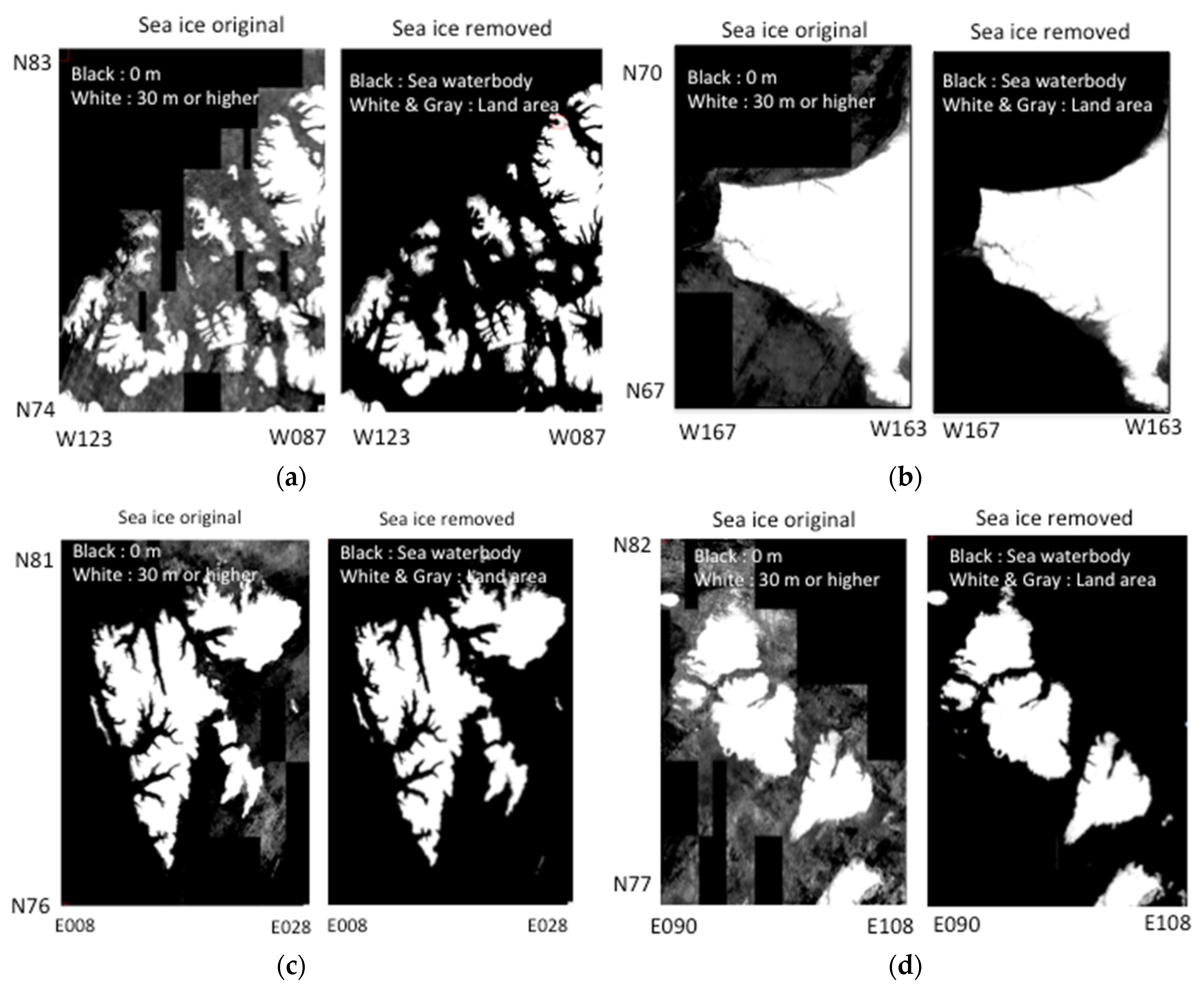
3. Sea-Waterbody
- (1)
- Latitudes of 60 degrees north and further north areas
- (2)
- Latitudes of 60 degrees south and further south areas
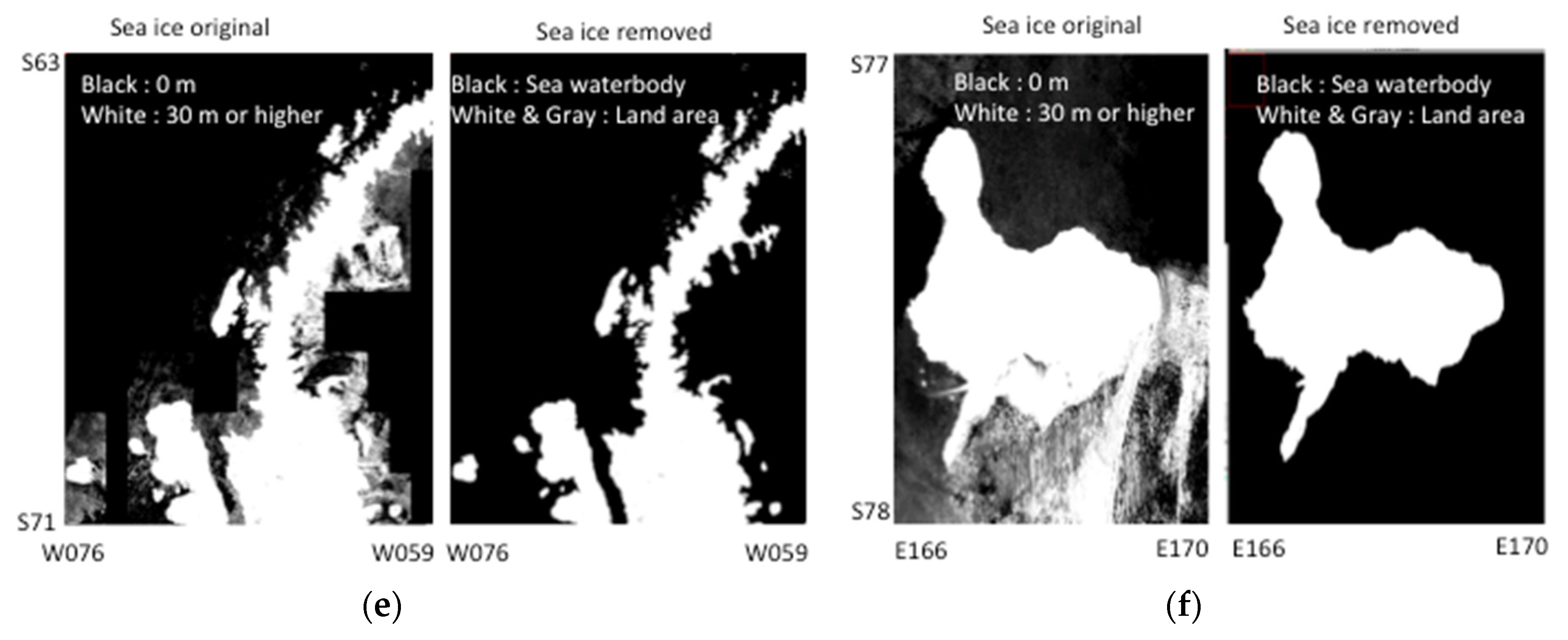
- (3)
- Extreme south of Greenland
- (4)
- Hudson Bay
- (5)
- James Bay
- (6)
- Ungava Bay
- (7)
- Sea of Okhotsk
- (8)
- Bering Sea
- (9)
- Patagonia area
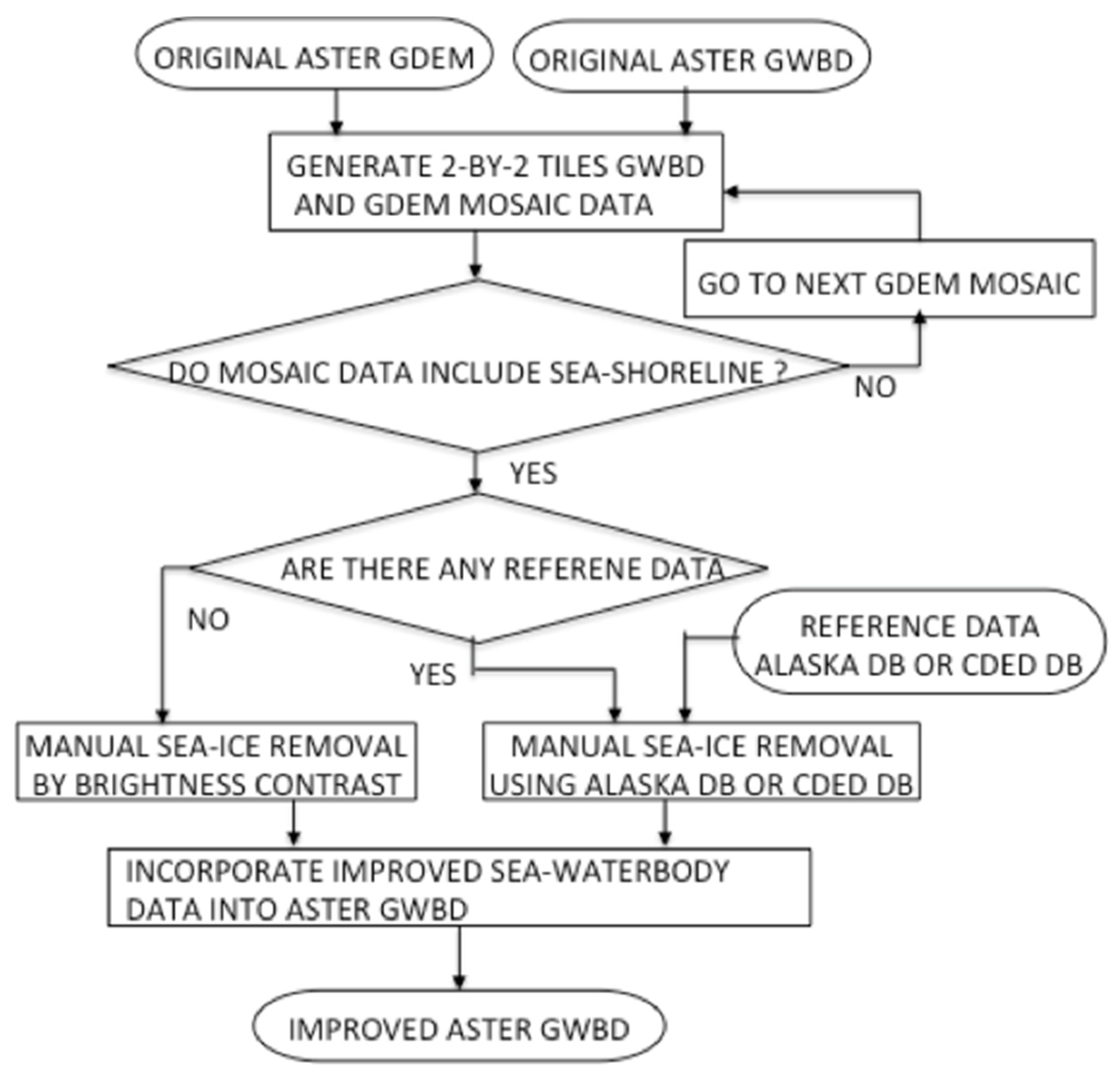
- (1)
- Generate a 2° latitude-by-2° longitude tile mosaic from unimproved Version 3 ASTER GDEM data.
- (2)
- If the mosaic area includes any sea shoreline, continue the processing.
- (3)
- If ancillary reference data exist in the mosaic area, delineate by comparing the mosaic data with the reference data by visual identification under the support tool. If reference data are not available, delineate by using brightness contrast under the support tool. In this case, the baseline technique is to designate all areas less than 30 m as sea ice, and then exclude land areas from the sea ice areas by comparing to Google Earth and GeoCover images and/or by visual judgments, as necessary and possible.
- (4)
- The improved sea-waterbody data were incorporated into the ASTER GWBD.
- (5)
- Repeat step (1) to step (4) for all sea ice removal target areas.
4. Lake-Waterbody
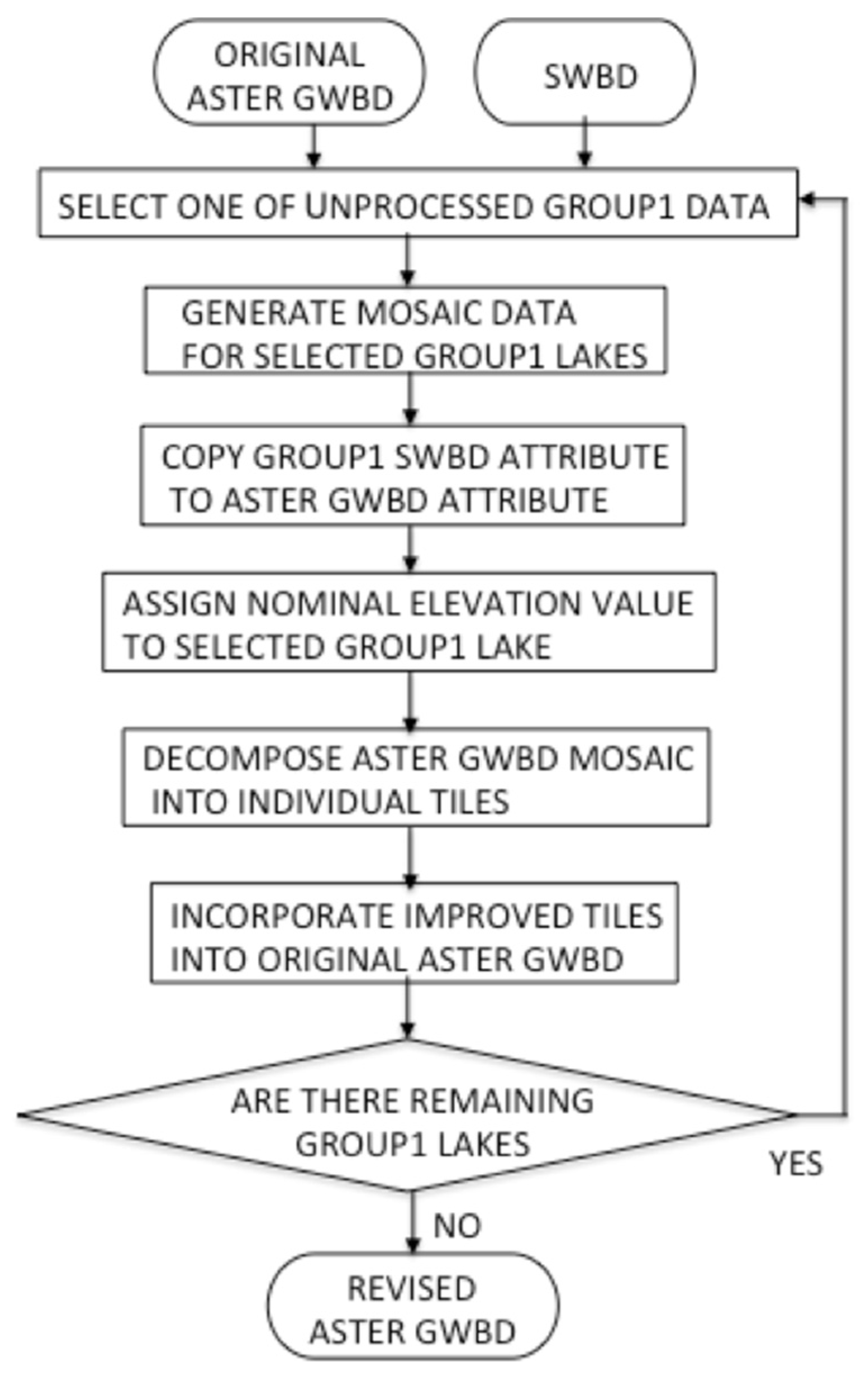
4.1. Processing Algorithm for Group1 Lake Waterbodies
- (1)
- Input original ASTER GWBD and SWBD.
- (2)
- Select one of the seven group1 lakes for correction.
- (3)
- Generate mosaic image data from both the input ASTER GWBD and the SWBD that cover the total area of the selected group1 lake.
- (4)
- Copy the selected group1 lake SWBD attributes to the corresponding ASTER GWBD attribute nuarea.
- (5)
- Assign the nominal elevation value in Table 2 to the selected group1 lake.
- (6)
- Decompose the ASTER GWBD mosaic image data into individual tiles.
- (7)
- Incorporate the improved tiles into original input ASTER GWBD.
- (8)
- If uncorrected group1 lakes remain, repeat Step (2) to Step (7).
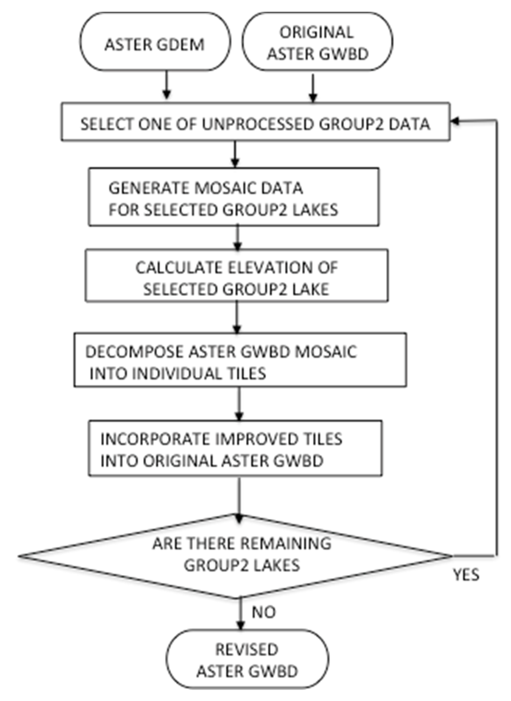
4.2. Processing Algorithm for Group2 Lake Waterbodies
- (1)
- Input original ASTER GWBD and ASTER GDEM.
- (2)
- Select one of the group2 lakes for correction.
- (3)
- Generate mosaic image data from both the unimproved input ASTER GWBD and unimproved ASTER GDEM that cover the total area of the selected group2 lake.
- (4)
- Calculate the elevation value of the selected lake surface by averaging perimeter elevations from the input ASTER GDEM data, using only the 10% of perimeter values that fall between 45% and 55% of the perimeter elevations in ascending order from the bottom to top, since the perimeter elevations have the random errors, and the center value is close to real value without the random errors. The parameter 10% is empirically selected.
- (5)
- Decompose ASTER GWBD mosaic image data into individual tiles.
- (6)
- Incorporate the improved tiles into original input ASTER GWBD.
- (7)
- If uncorrected group2 lakes remain, repeat Step (2) to Step (6).
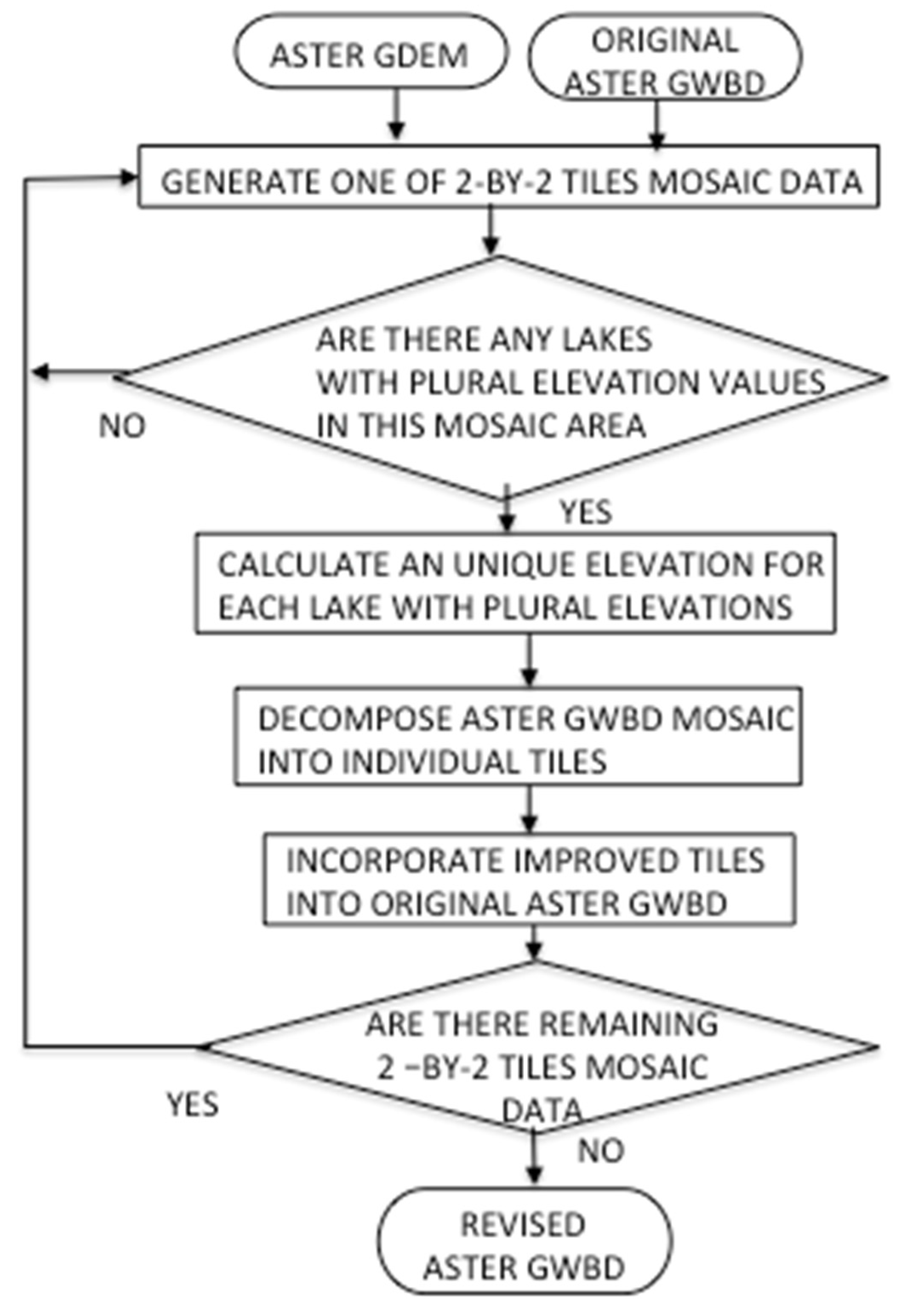
4.3. Processing Algorithm for Group3 Lake Waterbodies
- (1)
- Input the unimproved Version 3 ASTER GWBD and ASTER GDEM.
- (2)
- Generate a 2° latitude-by-2° longitude tiles mosaic image data from both the input ASTER GWBD and the ASTER GDEM.
- (3)
- If any lake in the mosaic area has plural elevations, go to next step to calculate the unique elevation for each abnormal lake. Otherwise, return to previous Step (2) to generate the next mosaic image data.
- (4)
- Calculate the unique elevation value for each abnormal lake with plural elevations by averaging the perimeter elevation data. For averaging, use only the data between 45% and 55% from the bottom in ascending order by the same reason as the group2 lakes.
- (5)
- Decompose ASTER GWBD mosaic image data into individual tiles.
- (6)
- Incorporate the improved tiles into the original input ASTER GWBD.
- (7)
- Repeat Step (2) to Step (6) for all land areas between latitudes 83°N and 83°S.
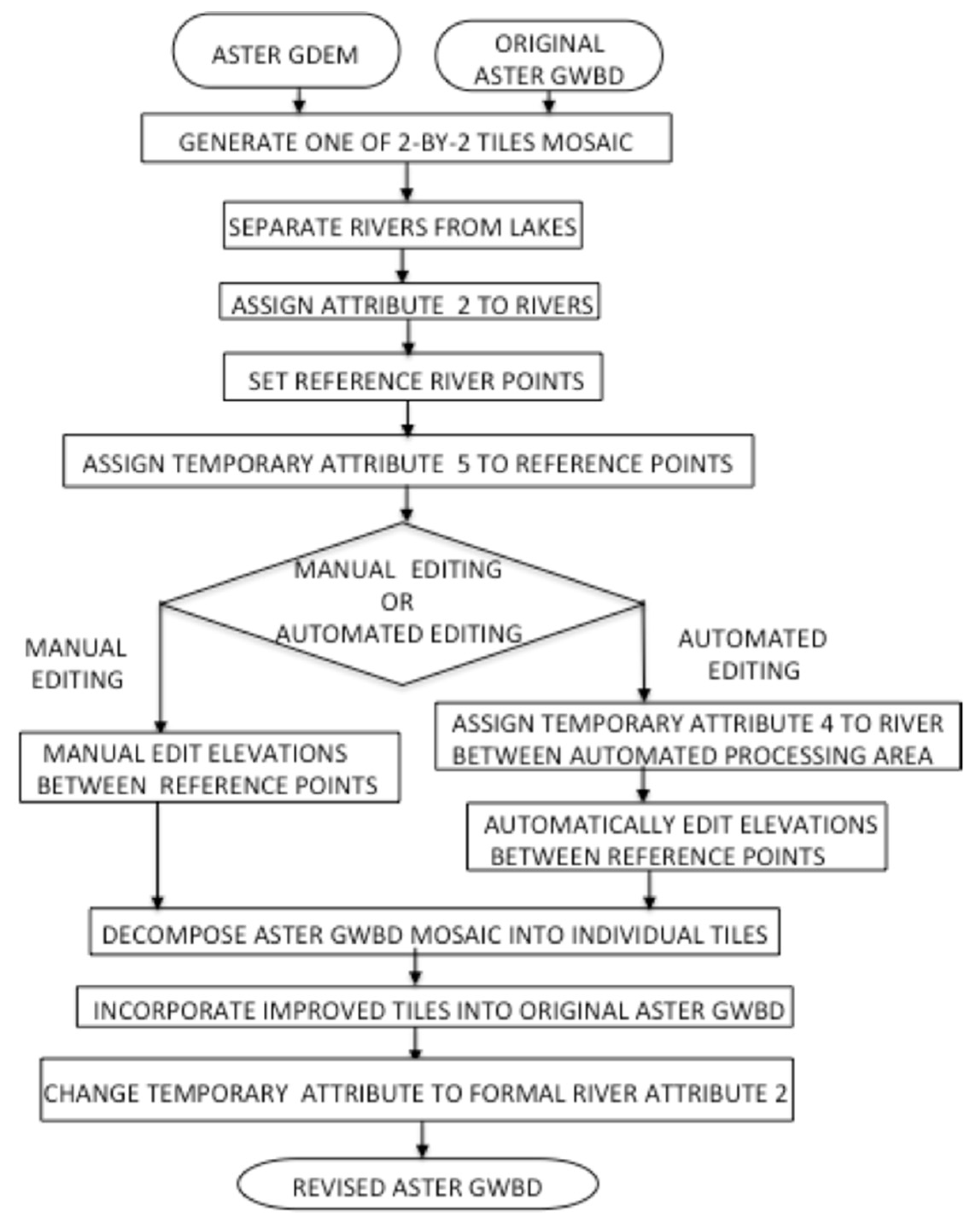
5. River-Waterbody
5.1. Basic Algorithm Flow for River Stepwise Elevation
- (1)
- Input original ASTER GWBD and ASTER GDEM.
- (2)
- Generate one of 2° latitude-by-2° longitude tiles mosaic image data from both the unimproved input ASTER GWBD and the ASTER GDEM.
- (3)
- Manually separate rivers from lakes, if any rivers exist.
- (4)
- Designate all existing rivers as nominal attribute 2.
- (5)
- Select river reference points from which stepwise elevations between adjacent reference points will be calculated by manual or automated editing, depending on the situation. Set reference point elevations based on perimeter data or SWBD data.
- (6)
- Temporarily designate river reference points as attribute 5.
- (7)
- Apply manual or automated editing to calculate stepwise elevations between adjacent reference points, using the support program.
- (8)
- Decompose ASTER GWBD mosaic image data into individual tiles.
- (9)
- Incorporate improved tiles into original input ASTER GWBD.
- (10)
- Change temporary attribute 5 to formal river attribute 2.
- (11)
- Repeat Step (2) to Step (10) for all land areas between latitudes 83°N and 83°S.
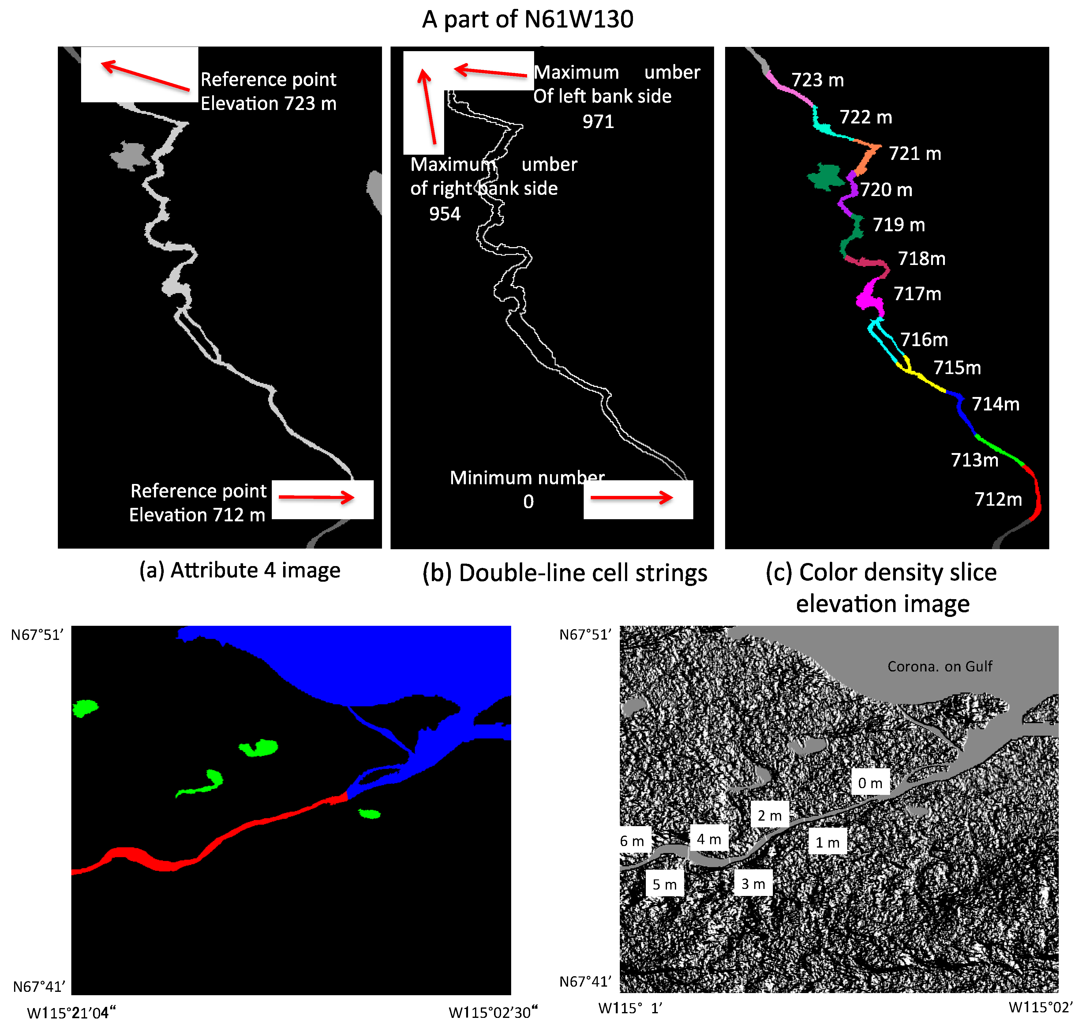
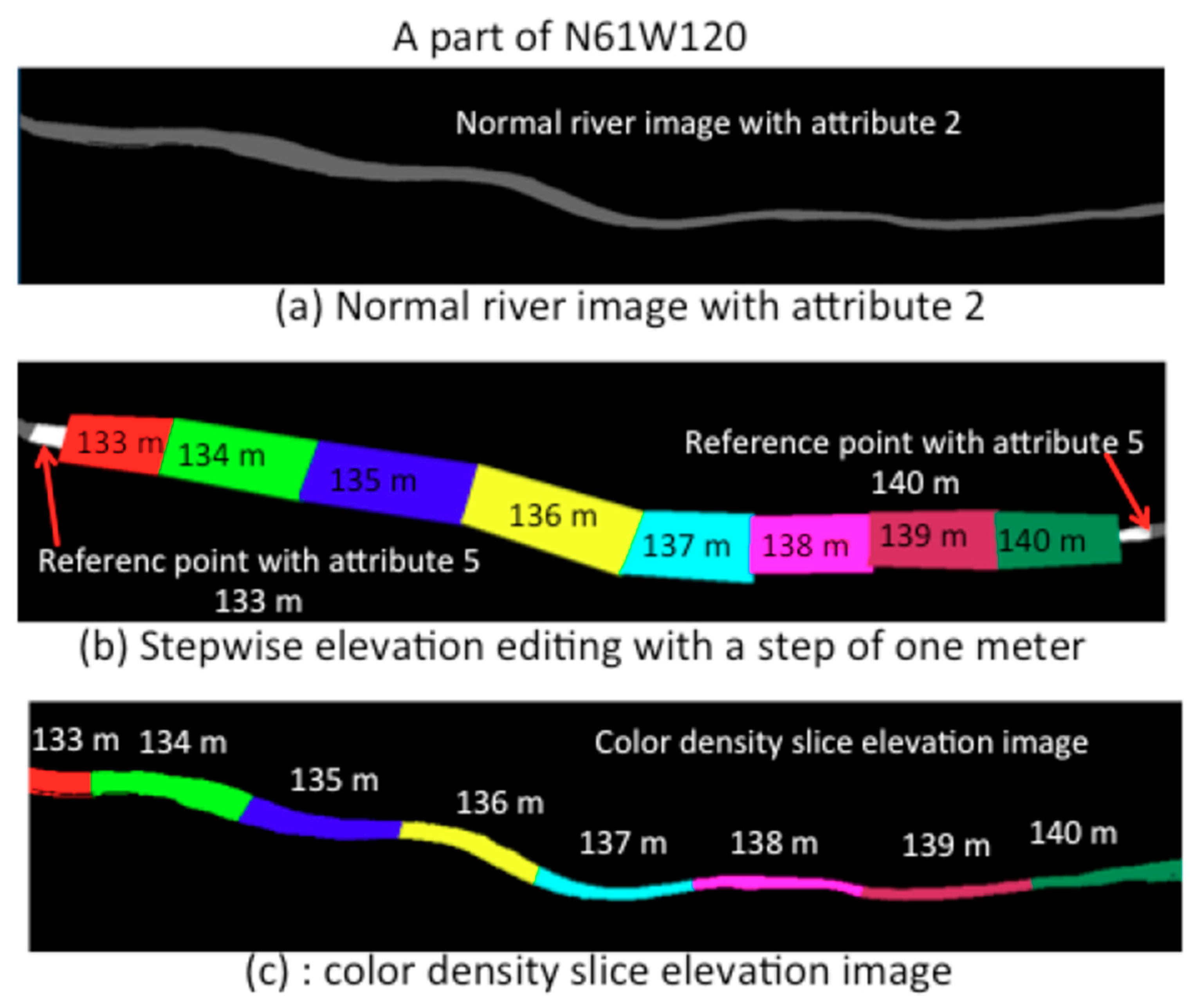
5.2. Manual Stepwise Elevation Editing
- (1)
- Original river image for stepwise elevation editing is first masked for each elevation value as shown in Figure 8b using the support tool. The elevation difference is roughly allocated in equal distance between adjacent reference points.
- (2)
- The attribute image area for each elevation value is selected by logical and operation for each masked area and attribute 2 area.
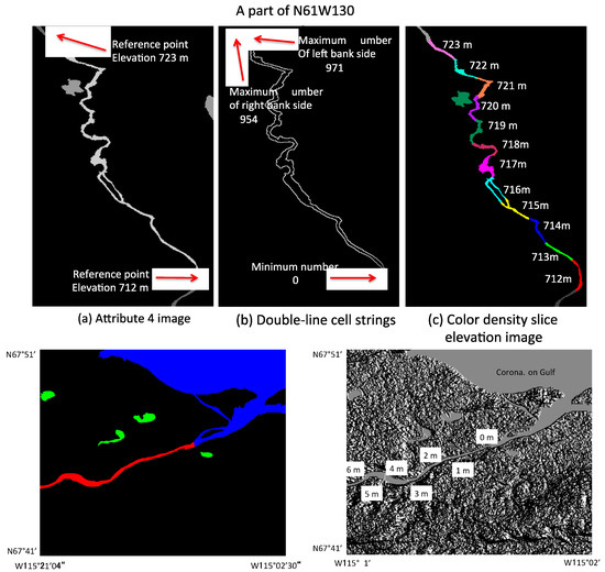
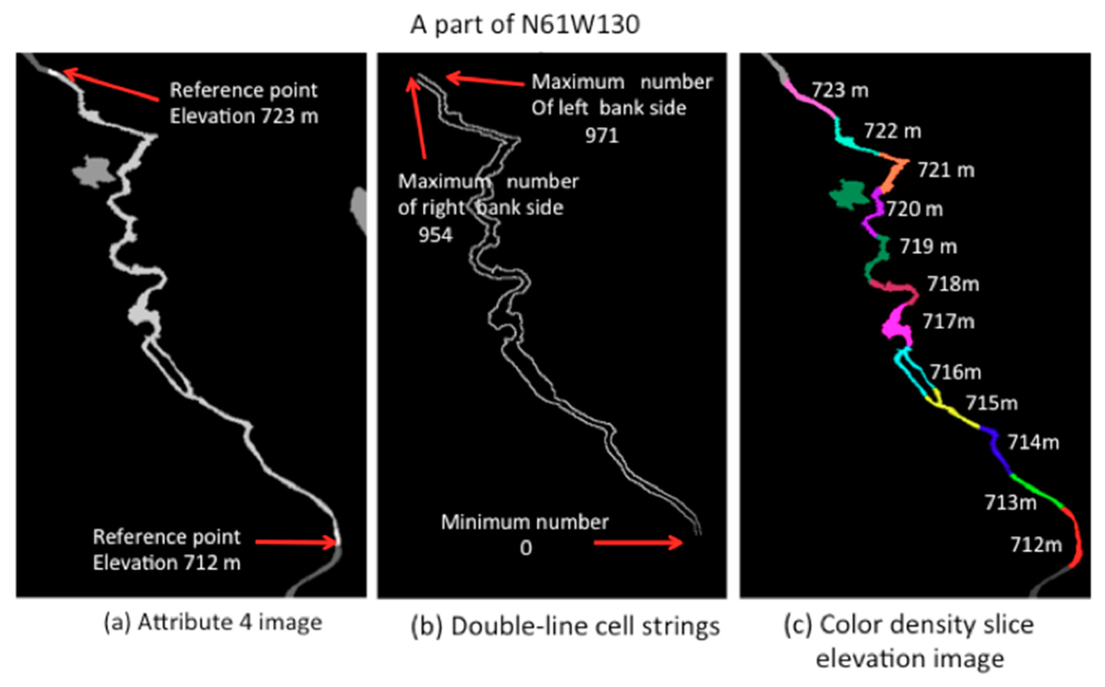
5.3. Automated Stepwise Elevation Editing
- (1)
- Assign the river area between adjacent reference points as temporary attribute 4 to designate the automated stepwise elevation editing area, including the start point (Figure 9a).
- (2)
- (3)
- Number each cell-string boundary line adjacent to the river from one reference point with the lowest elevation to the other reference points with the highest elevation. The starting minimum number is zero. The total numbers on the left bank side and right bank side may be slightly different, because the two banks of the river do not have exactly the same shoreline distance between reference points.
- (4)
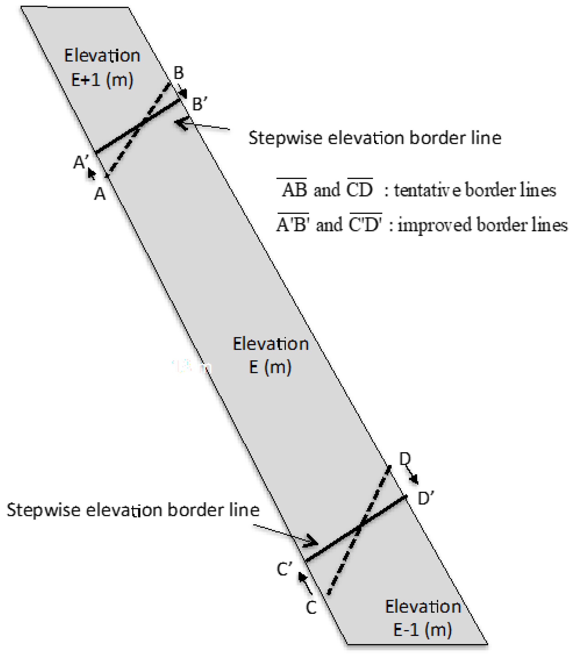
- Allocate consecutive cell string numbers for each one-meter step to calculate the borders at both bank sides and define the stepwise river segments. Tentative borderlines on the river are connecting lines between two positions ( and lines) at left and right banks as shown in Figure 10.
- (5)
- Rotate all border lines to have the shortest path lengths, since the borderlines with the shortest lengths are virtually at right angles to the river flow directions.
- (6)
- Assign the corresponding elevation values to all river sections between adjacent borders.
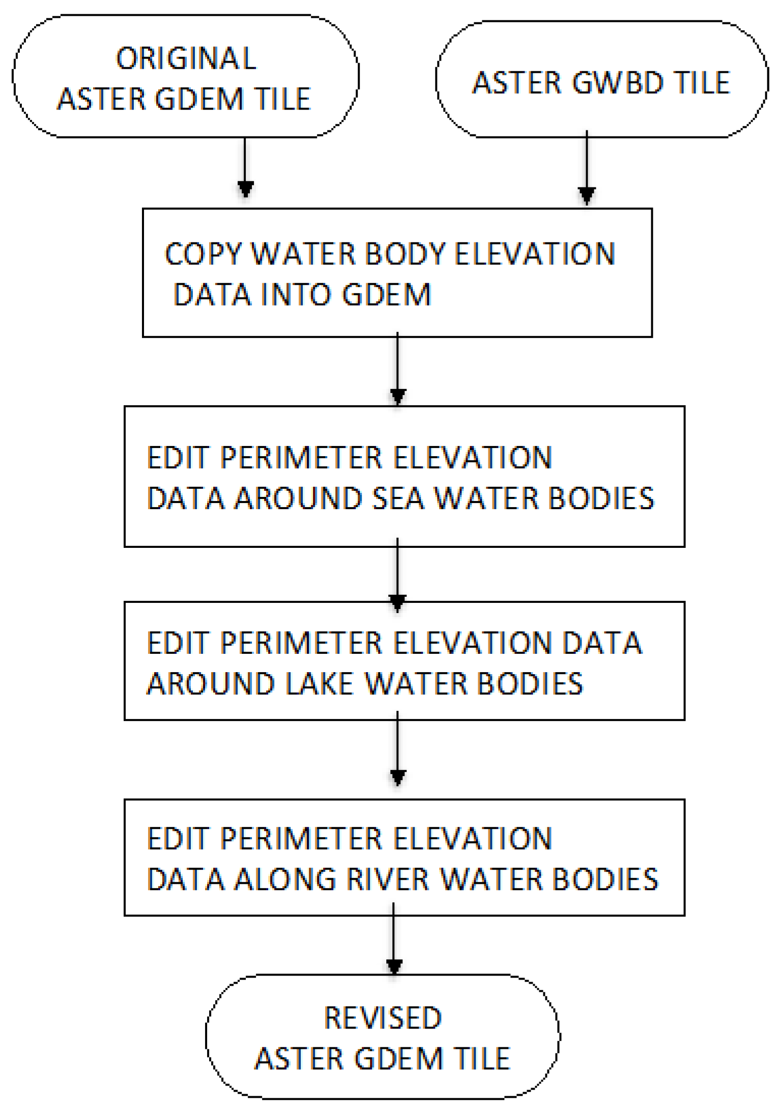
6. Incorporation of Waterbody Data into GDEM
- (1)
- Input original Version 3 ASTER GDEM and the now improved ASTER GWBD.
- (2)
- Select one ASTER GWBD tile and the corresponding original ASTER GDEM tile.
- (3)
- Copy the waterbody elevation data into the original ASTER GDEM tile.
- (4)
- Edit the land elevations along sea shorelines such that those are equal to or higher than one meter.
- (5)
- Edit the perimeter elevations for all lakes in the tile such that those are at least one meter higher than the lake elevation values.
- (6)
- Edit the perimeter elevations for all one-meter steps of rivers in the tile such that those are at least one meter higher than the elevations of the one-meter step area.
- (7)
- Repeat Step (2) to Step (6) for all ASTER GWBD tiles.
7. Summary
Author Contributions
Funding
Acknowledgments
Conflicts of Interest
References
- Fujisada, H.; Sakuma, F.; Ono, A.; Kudo, M. Design and preflight performance of ASTER instrument protoflight model. IEEE Trans. Geosci. Remote Sens. 1999, 36, 1152–1160. [Google Scholar] [CrossRef]
- Fujisada, H. ASTER Level-1 data processing algorithm. IEEE Trans. Geosci. Remote Sens. 1998, 36, 1101–1112. [Google Scholar] [CrossRef]
- Fujisada, H.; Bailey, G.B.; Kelly, G.G.; Hara, S.; Abrams, M.J. ASTER DEM performance. IEEE Trans. Geosci. Remote Sens. 2005, 43, 2707–2714. [Google Scholar] [CrossRef]
- Fujisada, H.; Iwasaki, A.; Hara, S. ASTER stereo system performance. Proc. SPIE 2001, 4540, 39–49. [Google Scholar]
- Fujisada, H.; Urai, M.; Iwasaki, A. Advanced methodology for ASTER DEM generation. IEEE Trans. Geosci. Remote Sens. 2011, 49, 5080–5091. [Google Scholar] [CrossRef]
- Fujisada, H.; Urai, M.; Iwasaki, A. Technical methodology for ASTER global DEM. IEEE Trans. Geosci. Remote Sens. 2012, 50, 3725–3736. [Google Scholar] [CrossRef]
- Carroll, M.L.; Townshend, J.R.; DiMiceli, C.M.; Noojipady, P.; Sohlberg, R.A. A new global raster water mask at 250 m resolution. Int. J. Digit. Earth 2009, 2, 291–308. [Google Scholar] [CrossRef]
- Feng, M.; Sexton, J.O.; Channan, S.; Townshend, J.R. A global, high-resolution (30-m) inland water body dataset for 2000: First results of a topographic–spectral classification algorithm. Int. J. Digit. Earth 2015. [Google Scholar] [CrossRef]
- Verpoorter, C.; Kutser, T.; Seekell, D.A.; Tranvik, L.J. A global inventory of lakes based on high-resolution satellite imagery. Geophys. Res. Lett. 2014, 41, 6396–6402. [Google Scholar] [CrossRef]
- Verpoorter, C.; Kutser, T.; Tranvik, L. Automated mapping of water bodies using Landsat multispectral data. Limnol. Oceanogr. Methods 2012, 10, 1037–1050. [Google Scholar] [CrossRef]
- Pekel, J.; Cottam, A.; Gorelick, N.; Belward, A.S. High-resolution mapping of global surface water and its longterm changes. Nature 2016, 540, 418–422. [Google Scholar] [CrossRef] [PubMed]
- SRTM Data Editing Rules, Version 2.0. 2003. Available online: https://dds.cr.usgs.gov/srtm/version2_1/Documentation/SRTM_edit_rules.pdf (accessed on 2 November 2018).
- SRTM Water Body Data Product Specific Guidance, Version 2.0. 2003. Available online: https://dds.cr.usgs.gov/srtm/version2_1/SWBD/SWBD_Documentation/SWDB_Product_Specific_Guidance.pdf (accessed on 2 November 2018).
- Slater, J.A.; Garvey, G.; Johnston, C.; Haase, J.; Heady, B.; Kroenung, G.; Little, J. The SRTM Data Finishing Process and Products. Photogramm. Eng. Remote Sens. 2006, 72, 237–247. [Google Scholar] [CrossRef]
- LandsatGeocoverMosaics. Available online: http://glcf.umd.edu/data/mosaic/ (accessed on 2 November 2018).
- GTOPO30. Available online: https://lta.cr.usgs.gov/GTOPO30 (accessed on 2 November 2018).
- Canada Digital Elevation Data. Available online: https://uwaterloo.ca/library/geospatial/collections/canadian-geospatial-data-resources/canada/canada-digital-elevation-data-cded (accessed on 2 November 2018).
- Alaska Digital Elevation Models. Available online: https://catalog.data.gov/dataset/5-meter-alaska-digital-elevation-models-dems-usgs-national-map78c4c (accessed on 2 November 2018).


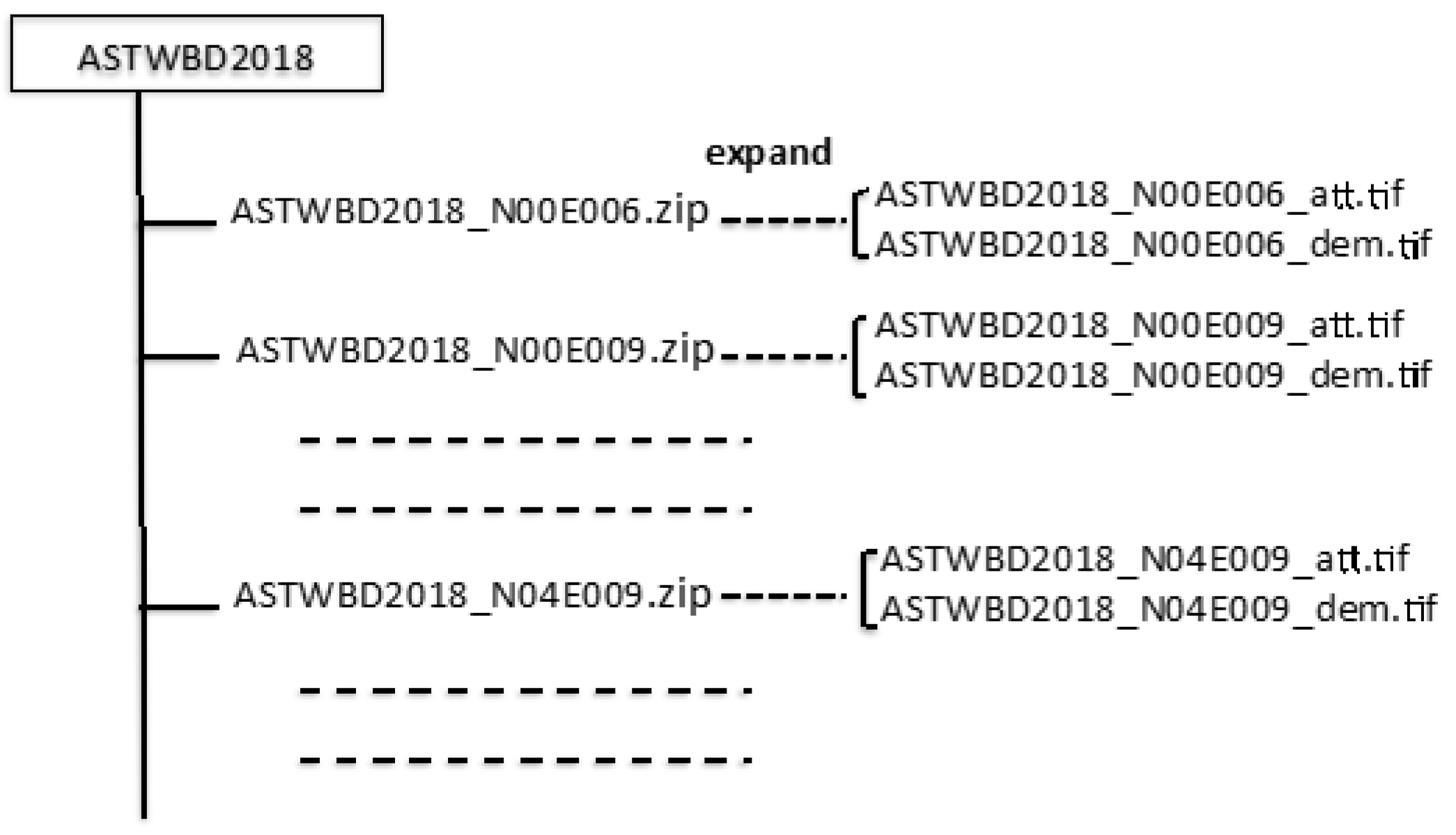
| Tile Size | 3601 × 3601 (1 degree by 1 degree) |
| Posting | 1 arc-second |
| Geographic coordinates | Geographic latitude and longitude |
| Geotiff, 8 bits for attribute | |
| Output format | Attribute DN values: 1 for sea, 2 for river, 3 for lake, and 0 for land |
| Geotiff, signed 16 bits, and 1 m/DN for dem files | |
| Special DN values | Referenced to the WGS84/EGM96 geoid |
| Coverage | North 83 degree to south 83 degree |
| Name | Location | ASTER GWBD | SWBD | ||
|---|---|---|---|---|---|
| Elevation (m) | Area (km^2) | Elevation (m) | Area (km^2) | ||
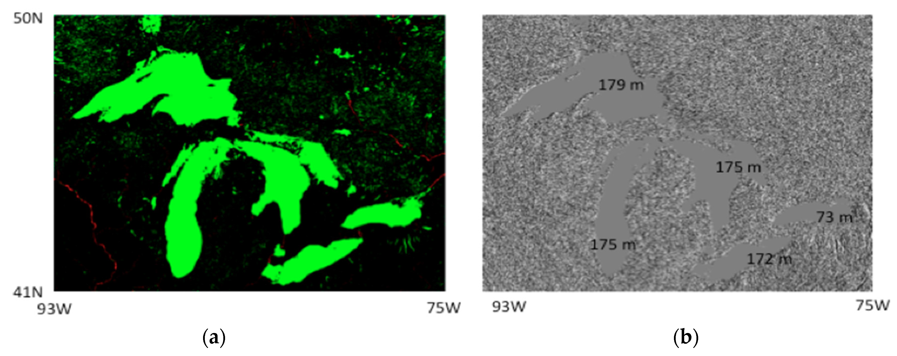
| Superior | USA, Canada | 179 | 81,482 | 179 | 81,330 |
| Michigan, Huron | USA, Canada | 175 | 118,659 | 175 | 118,490 |
| Erie | USA, Canada | 172 | 25,957 | 172 | 25,906 |
| Ontario | USA, Canada | 73 | 19,359 | 73 | 19,304 |
| Victoria | Kenya, Tanzania, Uganda | 1133 | 67,540 | 1134 | 67,455 |
| Bikal | Russia | 456 | 32,212 | 449 | 32,021 |
| Caspian | Russia etc. | −28 | 397,547 | −29 | 377,244 |
| Name | Location | ASTER GWBD | SWBD | ||
|---|---|---|---|---|---|
| Elevation (m) | Area (km^2) | Elevation (m) | Area (km^2) | ||
| Great Bear | Canada | 154 | 30,586 | - | - |
| Great Slave | Canada | 157 | 26,965 | - | - |
| Winnipeg | Canada | 215 | 24,396 | 215 | 24,370 |
| Manitoba | Canada | 237 | 4553 | 245 | 4578 |
| Winnipegosis | Canada | 250 | 5089 | 251 | 5157 |
| Cedar | Canada | 250 | 2553 | 253 | 2573 |
| Nipigon | Canada | 259 | 4464 | 258 | 4480 |
| Athabasca | Canada | 209 | 7697 | 207 | 7689 |
| Reindeer | Canada | 335 | 5258 | 335 | 5469 |
| Nettiling | Canada | 24 | 4744 | - | - |
| Amadjuak | Canada | 99 | 2813 | - | - |
| Churchill, Peter∙Pond | Canada | 413 | 1626 | 415 | 1796 |
| Kinbasket | Canada | 745 | 361 | 729 | 324 |
| Great Salt | USA | 1276 | 4434 | 1282 | 2770 |
| Nicaragua | Nicaragua | 34 | 7896 | 31 | 7868 |
| Titicaca | Bolivia, Peru | 3811 | 7654 | 3815 | 7549 |
| Vanern | Sweden | 41 | 5475 | 44 | 5459 |
| Vattern | Sweden | 95 | 1866 | 88 | 1870 |
| Peipsi | Estonia, Russia | 25 | 3497 | 28 | 3514 |
| Onega | Russia | 33 | 9784 | - | - |
| Name | Location | ASTER GWBD | SWBD | ||
|---|---|---|---|---|---|
| Elevation (m) | Area (km^2) | Elevation (m) | Area (km^2) | ||
| Ladoga | Russia | 3 | 17,688 | 4 | - |
| Aral Sea North | Russia etc. | 37 | 3147 | 39 | 3031 |
| Aral Sea South | Russia etc. | 26 | 18,333 | 29 | 23,743 |
| Yssyk-kol | Kyrgyuzstan | 1603 | 6224 | 1601 | 6217 |
| Balkhash | Kazakhstan | 337 | 17,341 | 338 | 17,053 |
| Volta | Ghana | 75 | 6329 | 75 | 6140 |
| Turkana | Kenya, Ethiopia | 348 | 7490 | 361 | 7512 |
| Tanganyika | Tanzania etc. | 773 | 32,971 | 767 | 62,971 |
| Malawi | Tanzaniaf, Malawi Mozambique | 476 | 29,688 | 476 | 29,653 |
| Kariba | Zambia, Zimbabwe | 482 | 5287 | 487 | 5349 |
| Bratsk1 | Russia | 293 | 4600 | 291 | 4831 |
| Bratsk2 | Russia | 392 | 1798 | 391 | 1850 |
| Krasnoyarskoye | Russia | 236 | 1920 | 223 | 1678 |
| Vilyuy | Russia | 234 | 2072 | - | - |
| Svetogorskaye | Russia | 83 | 497 | - | - |
| Hantalka | Russia | 48 | 2235 | - | - |
| Khantaiskoe | Russia | 57 | 1007 | - | - |
| Keta | Russia | 77 | 461 | - | - |
| Dyupkun | Russia | 102 | 240 | - | - |
| Taymyr | Russia | 5 | 4829 | - | - |
© 2018 by the authors. Licensee MDPI, Basel, Switzerland. This article is an open access article distributed under the terms and conditions of the Creative Commons Attribution (CC BY) license (http://creativecommons.org/licenses/by/4.0/).
Share and Cite
Fujisada, H.; Urai, M.; Iwasaki, A. Technical Methodology for ASTER Global Water Body Data Base. Remote Sens. 2018, 10, 1860. https://doi.org/10.3390/rs10121860
Fujisada H, Urai M, Iwasaki A. Technical Methodology for ASTER Global Water Body Data Base. Remote Sensing. 2018; 10(12):1860. https://doi.org/10.3390/rs10121860
Chicago/Turabian StyleFujisada, Hiroyuki, Minoru Urai, and Akira Iwasaki. 2018. "Technical Methodology for ASTER Global Water Body Data Base" Remote Sensing 10, no. 12: 1860. https://doi.org/10.3390/rs10121860
APA StyleFujisada, H., Urai, M., & Iwasaki, A. (2018). Technical Methodology for ASTER Global Water Body Data Base. Remote Sensing, 10(12), 1860. https://doi.org/10.3390/rs10121860