Article

Improving the Accuracy of Open Source Digital Elevation Models with Multi-Scale Fusion and a Slope Position-Based Linear Regression Method

1
School of Environment Science and Spatial Informatics, China University of Mining and Technology, Xuzhou 221116, China
2
Geographic Information and Tourism College, Chuzhou University, Chuzhou 239000, China
3
Science and Technology Development Department, Shenhua Group Corporation Limited, Beijing 100011, China
*
Author to whom correspondence should be addressed.
Remote Sens. 2018, 10(12), 1861; https://doi.org/10.3390/rs10121861
Submission received: 19 October 2018 / Revised: 14 November 2018 / Accepted: 17 November 2018 / Published: 22 November 2018
(This article belongs to the Special Issue Multi-Scale Remote Sensing and Image Analysis)

Abstract

:
The growing need to monitor changes in the surface of the Earth requires a high-quality, accessible Digital Elevation Model (DEM) dataset, whose development has become a challenge in the field of Earth-related research. The purpose of this paper is to improve the overall accuracy of public domain DEMs by data fusion. Multi-scale decomposition is an important analytical method in data fusion. Three multi-scale decomposition methods—the wavelet transform (WT), bidimensional empirical mode decomposition (BEMD), and nonlinear adaptive multi-scale decomposition (N-AMD)—are applied to the 1-arc-second Shuttle Radar Topography Mission Global digital elevation model (SRTM-1 DEM) and the Advanced Land Observing Satellite World 3D—30 m digital surface model (AW3D30 DSM) in China. Of these, the WT and BEMD are popular image fusion methods. A new approach for DEM fusion is developed using N-AMD (which is originally invented to remove the cycle from sunspots). Subsequently, a window-based rule is proposed for the fusion of corresponding frequency components obtained by these methods. Quantitative results show that N-AMD is more suitable for multi-scale fusion of multi-source DEMs, taking the Ice Cloud and Land Elevation Satellite (ICESat) global land surface altimetry data as a reference. The fused DEMs offer significant improvements of 29.6% and 19.3% in RMSE at a mountainous site, and 27.4% and 15.5% over a low-relief region, compared to the SRTM-1 and AW3D30, respectively. Furthermore, a slope position-based linear regression method is developed to calibrate the fused DEM for different slope position classes, by investigating the distribution of the fused DEM error with topography. The results indicate that the accuracy of the DEM calibrated by this method is improved by 16% and 13.6%, compared to the fused DEM in the mountainous region and low-relief region, respectively, proving that it is a practical and simple means of further increasing the accuracy of the fused DEM.

1. Introduction

DEMs are the fundamental tools of geo-analysis and the essential input variables for many models. They have been widely used in science and engineering fields such as water resource management [1,2,3], agriculture [4,5], and ecology [6,7,8]. DEMs can be derived not only from scanned/vectorized contour lines of existing topographic sheets obtained by field measurement [9], but also from remote sensing techniques. While the accuracy of the field measurement method is quite high, it is also time consuming and costly, especially in hard-to-reach areas [10,11]. Remote sensing has become the primary means of obtaining DEMs due to its near ideal characteristics in terms of coverage, and spatial and temporal resolution [12].
Owing to their high resolution (1 arc-second) and free access to download, the two most widely used quasi-global digital elevation models produced by remote sensing technology are the SRTM-1 DEM and the ASTER GDEM v2 [13]. The ASTER GDEM v2 is produced by optical stereoscopy [14], while the SRTM-1 DEM is based on the interferometric synthetic aperture radar technique, called InSAR [15]. They are widely applied in various fields because of their availability rather than their accuracy [16]. Unfortunately, all DEMs contain errors owing to the methods of collection and processing of the images that are used to produce them [2]. Their accuracy can lead to problems that are experienced in local and regional analyses [17].
To address these errors, many relevant studies have been conducted by many scholars. Rawat et al. [18] assessed the horizontal accuracy of ASTER GDEM, SRTM, and Castosat DEM with 20 GCPS and concluded that the three DEMs have different horizontal accuracy. Reinoso [19] provided an algorithm which automatically computed the horizontal shift for each contour set with same height between two DEMs. Further research by Reinoso et al. [20] estimated horizontal displacement between DEMs by means of particle image velocimetry techniques and pointed out that the largely ignored horizontal component had a great influence on the positional accuracy of certain linear features, e.g., in hydrological features. In another study, a simple and robust co-registration method presented for DEM pairs using the elevation difference residuals and the elevation derivatives of slope and aspect [21]. The method represented the complete analytical solution of a 3-D shift vector between two DEMs.
The DEM accuracy can be studied from the horizintal accuracy viewpoint as well as the vertical accuracy viewpoint. There has been much research into improving the vertical accuracy of DEMs. Some studies have aimed to improve the accuracy of the DEM by filling voids and removing the vegetation canopy [22,23,24]. Some other studies utilized geostatistical conflation techniques to increase the performance of DEM using a set of accurate Ground Control Points [25,26]. The research objects of these studies were single-source DEMs, and the inherent errors of the DEMs (depending on the method of data acquisition) cannot be eliminated. The interferometric synthetic aperture radar technique has the advantages of strong penetration ability and weak weather influence, but there remain problems with radar shadow, specular reflection, and phase unwrapping. This can lead to errors when the relief amplitude and surface roughness change abruptly (such as at peaks, cliffs, etc.). As for the DEM obtained by optical sensors, the data accuracies are affected by weather conditions such as cloud cover, mist occlusion, and so on [27]. The complementary error behaviors of optical stereoscopy and InSAR provide the possibility for DEM fusion [27]. Therefore, the integration of the two kinds of DEMs using data fusion can achieve this advantageous behavior and improve the accuracy of original DEMs.
To date, many methods of DEM fusion have been put forward. Fabris et al. [28] integrated bathymetric multibeam surveys with aerial photogrammetry and lidar surveys provided the first high resolution 3D terrestrial and marine morphological map of the Panarea volcano. An innovative method of weighted sum of data sources with geomorphologic enhancement was developed [29] to get a better DEM than any data source, which was visually and geomorphologically homogenous. In some other studies, scholars focus on the weighted average method of DEM fusion. Schultz et al. [30] implemented the fusion of multi-temporal DEMs, obtained by optical stereoscopy in the same region through self-consistency. Honikel [31] described the process of DEM fusion by weighting the values of two DEMs according to the estimation error, utilizing the advantages of InSAR and optical stereoscopy. Schindler et al. [32] improved the precision of large scale DEM data by weighted fusion, and pointed out the importance of weight to the fusion result. These studies looked at the DEM data as a whole and used weighted averages to improve the accuracy of the fused DEM, ignoring the different characteristics of the DEM data in various frequency domain scales. In another study, the original DEMs were transformed into the frequency domain, then high-pass and low-pass filters were used to fuse it, which achieved good results [33]. Nevertheless, details and texture information might be lost in the filtering process, which affects the ability of the DEM to describe micro-topography.
In most of the reported studies, DEM fusion was based on SRTM and ASTER. With the development of modern imaging technology, new high-resolution DEM products have been produced and released in recent years, such as the AW3D30 DSM [34,35], which also uses optical stereoscopy (with a resolution of 1 arc-second). It is the most accurate of the open source DEMs according to accuracy assessments, so it can be regarded as an alternative to the ASTER GDEM v2 [34,36]. Existing studies have showed that the impact of DEM resolution on the accuracy of terrain representation and of the gradient determined [37]. The representation accuracy decreases sharply at coarse resolutions. Therefore, further research is necessary to examine and apply DEM fusion techniques to newly-released high-resolution datasets such as the SRTM-1 and AW3D30. Besides, Honikel [38] suggested that the errors of the stereo optical DEMs and interferometric DEMs were shown in different frequency domains. Coincidentally, multi-scale analysis methods (e.g., the popular WT and BEMD) can decompose DEMs into different frequency domains. Thus, a rule-based fusion of DEMs based on multi-scale analysis methods makes sense.
This study aims at improving the overall accuracy of open source DEMs (the SRTM-1 and AW3D30) with complementary sensing technologies by multi-scale fusion. Due to the absence of reference DEM in the study area, the ICESat global land surface altimetry product, is used to assess the accuracy of the results. The basic parameters of the experimental data are shown in Table 1. Furthermore, the effectiveness of three multi-scale analysis methods (WT, BEMD, and N-AMD) in fusing DEMs is examined, based on the fusion rule mentioned in Section 3.2. Among these, N-AMD—which was originally invented to remove the cycle from sunspots—has proven superior to existing methods (e.g., chaos-based and wavelet-based approaches) in noise removal and trend determination [39,40,41]. Thus, it is considered to have potential for DEM multi-scale fusion because of its good performance. Finally, it is known that DEM accuracy varies for different slopes [16,42]. This suggests a further extension is possible by using the local variations in errors for different slope positions and a slope position-based linear regression method is proposed to use this information for the further calibration of fused DEM.

2. Study Area and Datasets
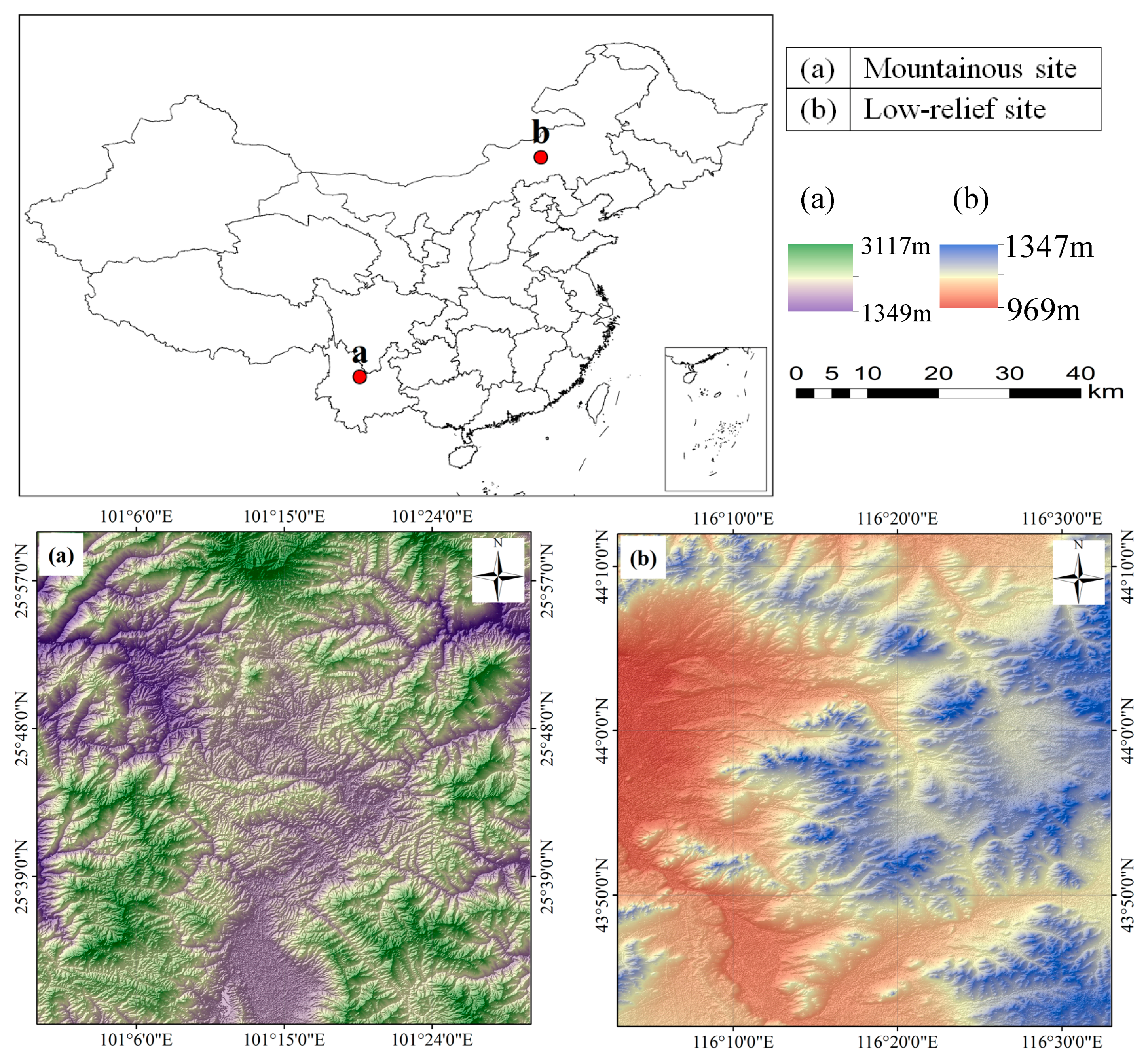
2.1. Study Area

Two regions in China are selected for research, as shown in Figure 1. Site A is located in the city of Chuxiong, Yunnan Province (101°–101.5°E, 25.5°–26°N) in Southwestern China. It is a typical mountainous area with a complex terrain. The flora mainly consists of perennial trees, and annual variation is not significant. Site B is located in Xilinhot, in the Inner Mongolia Province (116°–116.5°E, 43.7°–44.2°N) of Northern China. The landscape is mostly grassland, with a gentle undulating surface and annual dwarf herbs. Most of these two regions are inaccessible zones, and their geological conditions are relatively stable. The elevation fluctuations caused by human and natural factors can be ignored.

2.2. Datsets

In this paper, we integrate multisource DEMs to generate a fused DEM with higher accuracy. The data sources include the SRTM-1 DEM and AW3D30. In addition, the ICESat global land surface altimeter data is included for accuracy validation. The specific characteristics of the datasets are described below.

2.2.1. SRTM-1 DEM

The SRTM is a survey mission performed by NASA and the National Geospatial-Intelligence Agency (NGA) in an 11-day flight by the STS Endeavour OV-105 from February 11th, 2000 to February 22nd, 2000 [43]. It acquired land surface radar image data from 60°N to 56°S. The current SRTM DEM was generated by the NASA JPL Ground data processing system, using the C-band radar signal. The SRTM DEM can be divided according to precision into the SRTM-1 and SRTM-3, with corresponding resolutions of 30 m and 90 m, respectively. It is based on the WGS84 horizontal datum and EGM96 vertical datum. At 90% confidence level, the vertical error of the DEM is less than 16 m [44]. This study uses the SRTM-1 global dataset released in September 2014. This new dataset provides world-wide coverage of void-filled elevation data with high resolution (30 m). The URL for downloading the dataset is http://earthexplorer.usgs.gov/.

2.2.2. AW3D30

The AW3D is a new-generation, high-resolution global digital surface model dataset released by the Japan Aerospace Exploration Agency (JAXA) in 2016. It uses a panchromatic remote sensing instrument for stereo mapping (PRISM) on ALOS satellites to observe all regions of the land from 80°N to 80°S [45]. The elevation value is computed by DOGS-AP software, based on the location of an object in images taken from three different angles. Due to its late release time, there are few studies that assess the vertical accuracy of the AW3D. The AW3D30 is the most accurate open source DEM, and can be used as alternative data for the SRTM DEM and ASTER GDEM [34,36]. The AW3D is a digital elevation product with a resolution of 5 m, and the AW3D30 product can be obtained by resampling AW3D. Depending on the resampling mode, it can be divided into median and mean versions. The mean version is selected in this study and can be downloaded at http://www.eorc.jaxa.jp/ALOS/en/aw3d30/.

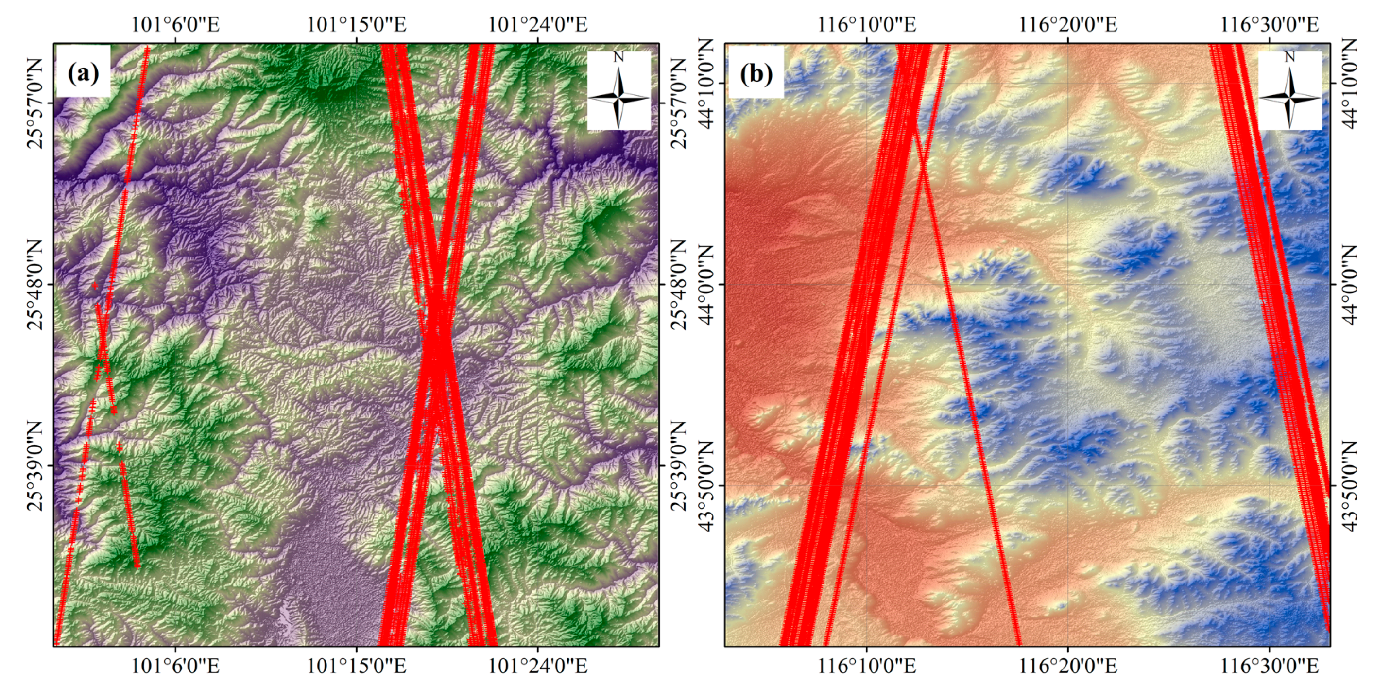
2.2.3. ICESat GLAH14

The geoscience laser altimeter system (GLAS) carried on board the ICESat, which was launched by NASA in January 2003, was principally designed for measuring ice sheet elevation and elevation changes over time [46]. The GLAS contains three different lasers that produce laser spots (with a diameter of approximately 70 m) on the Earth’s surface every 172 m in the along-track direction. The cross-track spacing varies depending on the latitude [47]. The horizontal accuracy of the laser spots is 6 m, while the vertical accuracy can be better than 15 cm [48,49]. In the current work, the GLAS/ICEsat L2 global land surface altimetry data version 34 (GLAH14) is utilized as reference data for the DEM accuracy assessment. However, outliers caused by poor weather conditions during data acquisition, such as cloud reflections, need to be removed before using the products [50,51], as discussed in Section 2.3.2. The dataset is freely available from NSIDC (www.nsidc.org).

2.3. Data Pre-Processing

2.3.1. DEM Processing

Due to the differences in geographic coordinate systems and pixel sizes of the SRTM-1 and AW3D30, co-registration is needed before accuracy assessment and DEM fusion [52]. Taking the SRTM-1 as reference, the elevation difference residuals and the elevation derivatives of slope and aspect are used to register these products, using the co-registration algorithm presented in [21].
The SRTM-1 produced by C-band radar signal can partially penetrate the vegetation canopy, while the AW3D30 produced by optical stereoscopy is not able to penetrate the canopy. Hence, the method described in [53] is used to distinguish vegetation areas from non-vegetation areas. Subsequently, the approximate vegetation height is estimated in the vegetation area, completing the DEMs calibration.

2.3.2. GLAH14 Processing
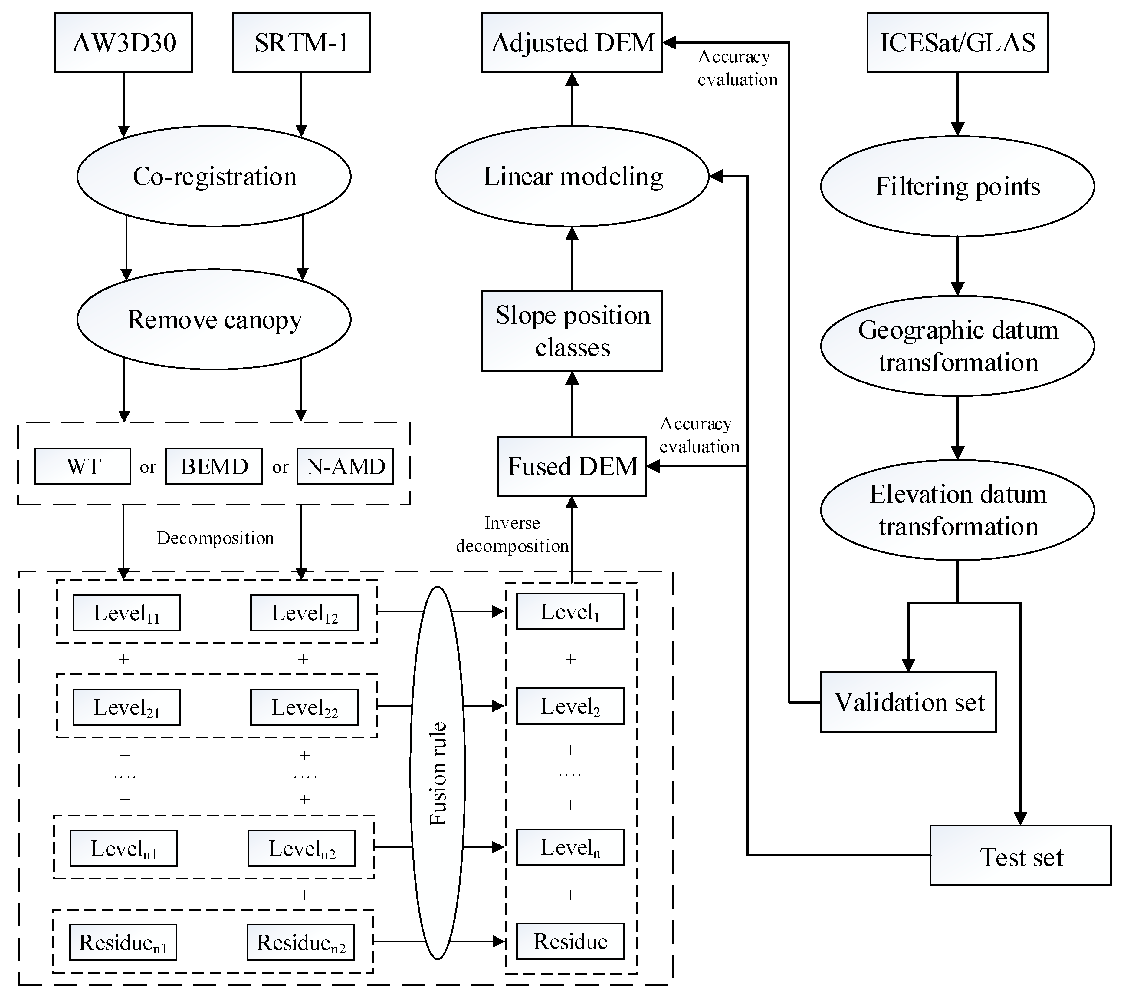
Previous studies have suggested that the horizontal displacements between the GLAH14 and three DEMs are small enough to be ignored [54]. Nevertheless, the elevations of the GLAH14 points are relative to the surface of the TOPEX/Poseidon reference ellipsoid, while the elevations of the SRTM-1 and AW3D30 are based on the EGM96 vertical datum. Therefore, pre-processing of the GLAH14 is needed to complete the conversion from TOPEX/Poseidon to WGS/EGM96. The difference between the geoid and T/P ellipsoid is provided in the GLAH14 data as N [55], such that:
H WGS 84 = h N ( o f f s e t )
where h is the elevation of the center of the laser point relative to the TOPEX/Poseidon ellipsoidal surface, and offset is the difference between the two ellipsoid height datum. The value of offset increases with latitude, and it varies within narrow range. Generally, offset is regarded as a constant. In this paper, the value is set to be 0.7 m.
After the height datum unification is complete, the laser points with excessive error—caused by cloud reflections and atmospheric noise during the time of the GLAH14 data acquisition—need to be removed. Selection of the GLAH14 points is implemented according to various criteria in different applications. There are many parameters provided by the GLAH14 data that can be used to implement the data selection. The main objective is to determine the laser points that meet the accuracy of the DEM assessment. Thus, a filtering criteria is chosen to filter error points, using parameters including the signal width and received energy [50,51]. Specifically, the received energy threshold is set to 10 fJ, while the signal width is 25 m. Furthermore, the points where the elevation difference between the GLAH14 and DEM is smaller than -100 m and greater than 100 m are also filtered as gross error. The distributions of the GLAH14 points in sites A and B after processing are shown in Figure 2. It can be seen that the distributions span the entire study area, covering almost all terrain types. Moreover, the GLAH14 set is divided into two parts: the test set and the validation set. The points of these two parts are (4147, 1712) and (5564, 2136) in sites A and B, respectively.

3. Methods

A DEM of higher quality can be generated using the following steps. Firstly, the open source DEMs (the SRTM-1 and AW3D30) are decomposed into n-level frequency domains (with a residue) by three methods (WT, BEMD, and N-AMD). Secondly, the fusion rule is applied to fuse each corresponding component. Thirdly, the fused components are combined into the fused DEM. Finally, the most accurate one is selected by comparing the accuracy of fused DEMs generated by three methods, before a slope position-based linear calibration is used to further improve the accuracy and obtain the adjusted DEM. The schematic flowchart of the process is shown in Figure 3.

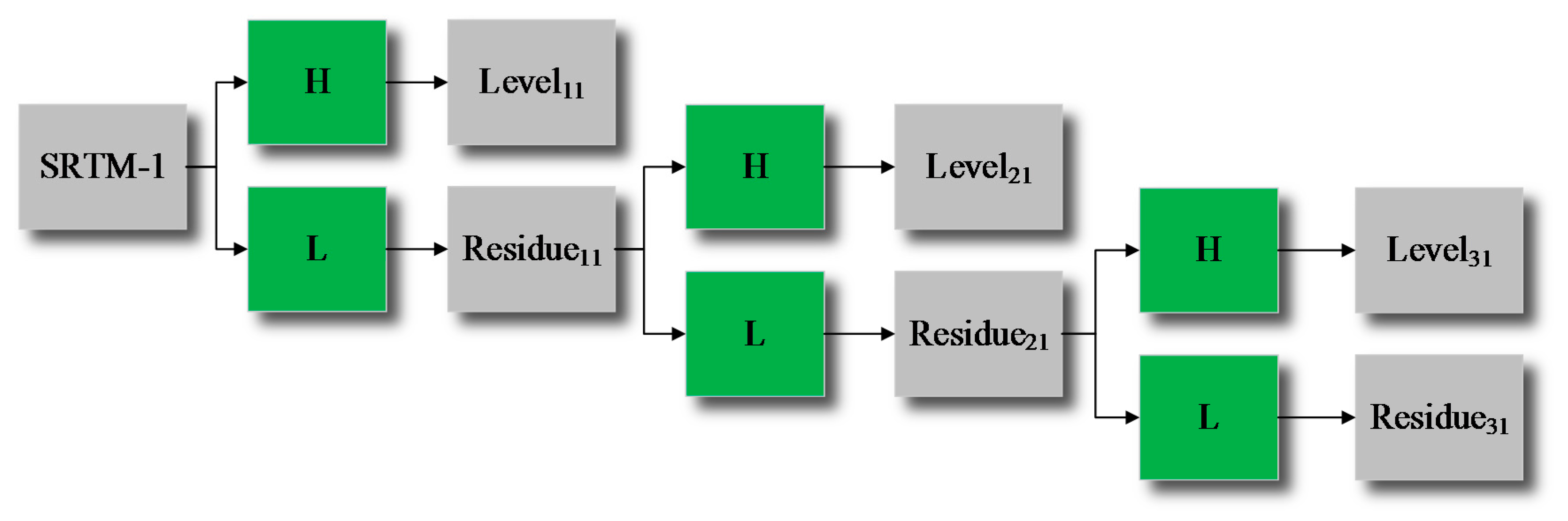
3.1. Multi-Scale Analysis Methods

3.1.1. Wavelet Transform (WT)

The wavelet transform is a widely used analysis method, which is called the “microscope” in mathematics. This method is a multi-resolution time-frequency analysis approach. In particular, it has high frequency resolution in the low-frequency section, and high time resolution in the high-frequency section [56,57]. Because of its adaptability and auto-focusing ability, the wavelet transform is especially suitable for non-stationary signal processing. Hence, it can be applied to the surveying field extensively [58].
The wavelet transform first moves the basis wavelet function, and then makes the inner product with the signal to be analyzed at different scales. The above process belongs to the category of wavelet decomposition and is invertible. The inverse process is called wavelet reconstruction. The expressions of wavelet decomposition and wavelet reconstruction are given by [59,60]:
W ψ ( a , b ) = x ( t ) , ψ = 1 | a | R x ( t ) ψ * ( t b a ) d t , a > 0
x ( t ) = K R W ψ ( a , b ) 1 | a | ψ ( t b a ) d a d b a 2 , a > 0
where Wψ(a, b) is the wavelet decomposition coefficient, x(t) is the data to be decomposed, ψ is the appropriate mother wavelet determined based on the data, ψ* is the complex conjugate of ψ, a is the scaling factor and b is the translation factor, and the angled brackets represent the inner product.
The schematic diagram of the SRTM-1 decomposition, using wavelet analysis, is shown in Figure 4. Three-level decomposition is illustrated as an example. H and L represent the high-frequency and low-frequency components, Residue11, Residue21, and Residue31 represent the 1st, 2nd, and 3rd layer of the approximation part, and Level11, Level21, and Level31 are the 1st, 2nd, and 3rd layer of the high-frequency part, respectively. It is seen that the wavelet transform can decompose the DEM in a coarse or fine manner, as well as splitting it into low and high frequency parts. In addition, each part has a relationship with the original DEM that is described by: SRTM-1 = Residue31 + Level31 + Level21 + Level11. Hence, wavelet analysis is an almost non-destructive signal analysis method.

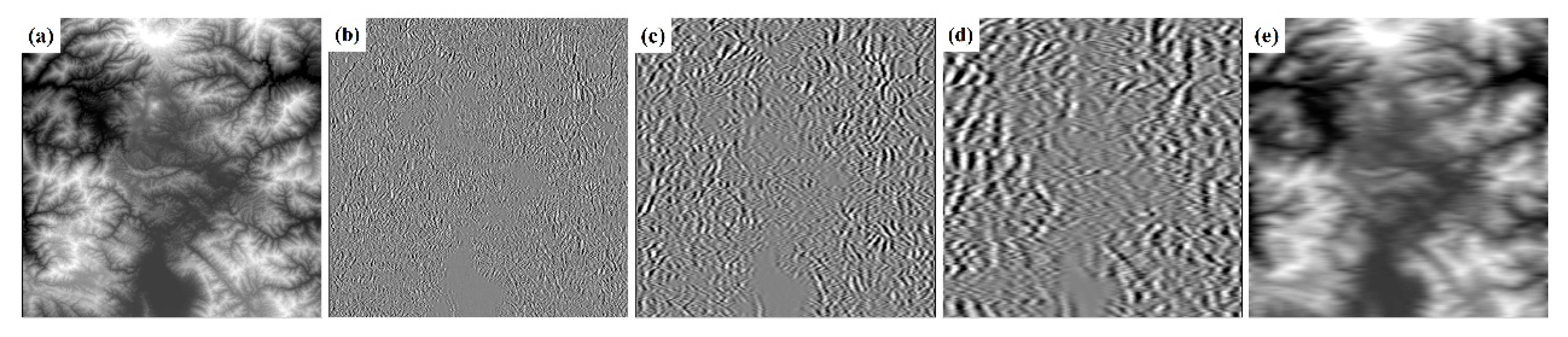
3.1.2. Bidimensional Empirical Mode Decomposition (BEMD)

Empirical mode decomposition (EMD) is a novel time-frequency analysis method proposed by Huang et al. [61]. This new technique is completely independent of the Fourier transform, and can be used for nonlinear, non-stationary signal linearization and smooth processing. It preserves the characteristics of the signal itself and is a completely data-driven time-frequency technique. An arbitrary signal will be decomposed into a set of multiple oscillatory components, called the intrinsic mode functions (IMFs), which contain the local features of the original signal at different time scales. BEMD is an extension of EMD for the processing of two-dimensional images [62]. BEMD extracts the details of the image first, and then the smooth region is screened out gradually. The entire process is similar to the WT method, except the results of the WT decomposition will differ depending on the various basis functions. BEMD can achieve image decomposition from a small to a large scale, under appropriate boundary conditions and termination criteria, without pre-setting the basis functions, making it more convenient and easy than the WT method. Since the number of zero-crossing points of the IMFs is not captured by statistics, the constraints of the IMFs or the Cauchy-type convergence condition can be used for BEMD as a termination criteria of the filtering process [61]. The process of decomposing an image into a series of IMFs and one Residue component using BEMD is as follows [62,63]:
Step 1:
Identify extreme points (both maxima and minima) of image I.
Step 2:
Generate upper and lower envelopes by interpolating the maximum and minimum points respectively.
Step 3:
Calculate the mean plane m of the two envelopes.
Step 4:
Extract the details using d = Im.
Step 5:
Repeat the above steps until d becomes an IMF.
After the above decomposition, the image is represented as:
I ( x , y ) = i = 1 n i m f i ( x , y ) + R n ( x , y )
where imfi (x, y) (i = 1, 2, …, n), are IMFs, and Rn(x, y) represents the Residue.

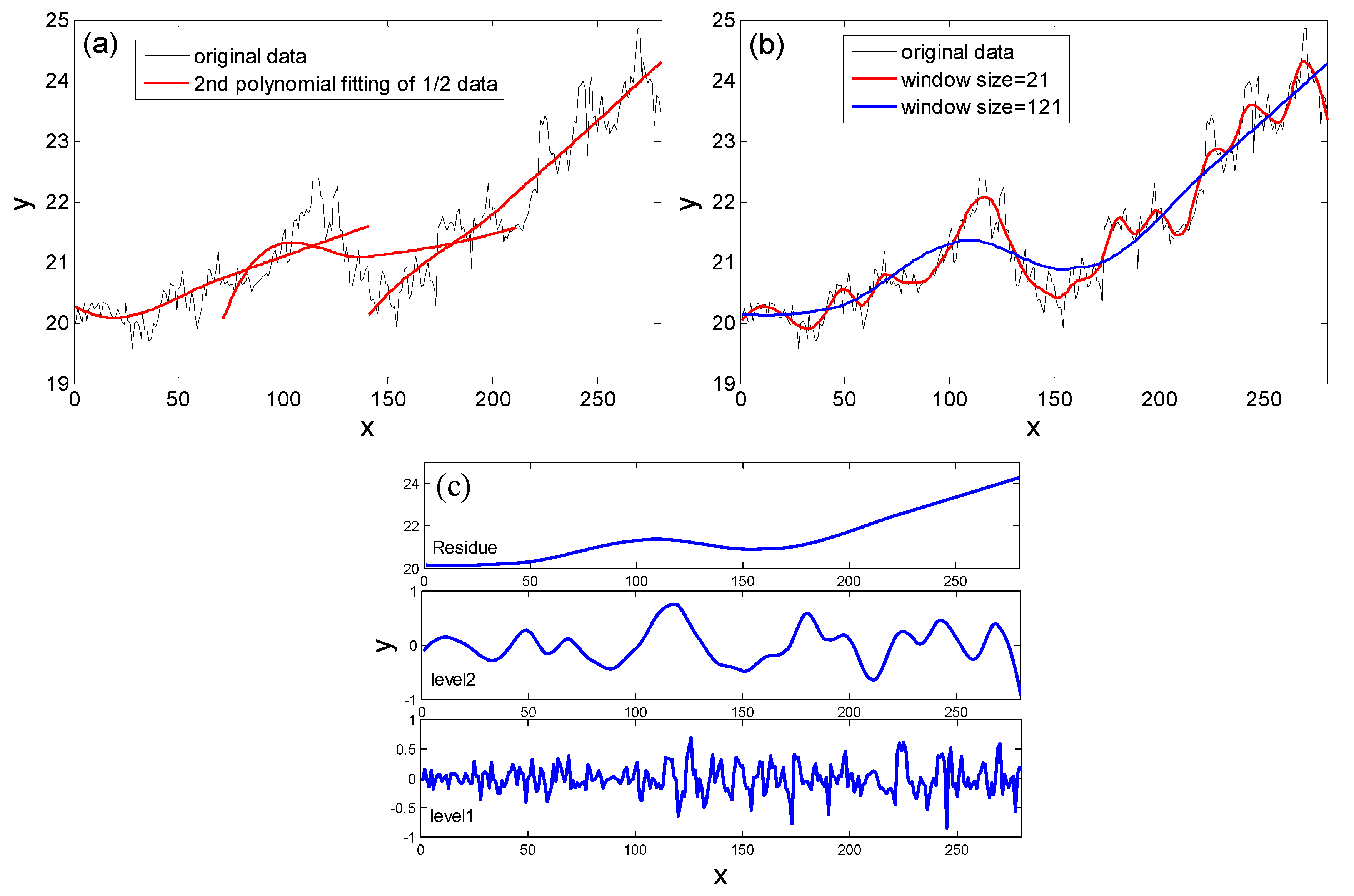
3.1.3. Nonlinear Adaptive Multi-Scale Decomposition (N-AMD)

Nonlinear adaptive multi-scale decomposition (N-AMD) is a new nonlinear adaptive multi-scale decomposition method proposed by Gao et al. [41] that can determine any trend signal without prior knowledge. It has been proven that the N-AMD can reduce the noise of time series data more effectively than the linear filters, wavelet shrinkage, and chaos-based noise reduction scheme [40]. It divides a time series into multiple parts of length of 2n + 1 with adjacent parts overlapping by n + 1, so the time scale introduced by the algorithm is n sampling points. Then K-polynomial fitting is applied to each part. In particular, K = 0 and 1 correspond to piecewise constants and linear fitting, respectively. The fitted polynomials for the i-th and (i + 1)-th parts are denoted by y(i)(l1) and y(I + 1)(l2), l1, l2 = 1, …, 2n + 1, and the fitting of the overlapped region is defined as:
y ( c ) ( l ) = w 1 y ( i ) ( l + n ) + w 2 y ( i + 1 ) ( l ) , l = 1 , 2 , , n + 1
where w1 = (1 − (l − 1)/(n)), w2 = (l − 1)/(n) can be written as (1 − dj/n), j = 1, 2 (dj represents the distances from the point to the centers of y(i) and y(i + 1), respectively). This means that the weight decreases linearly with distance from the point to the center of the line segment. This weighting ensures symmetry and effectively eliminates any jumps or discontinuities on adjacent segment boundaries. In fact, the scheme ensures that the fitting is smooth at the non-boundary point and has a right or left derivative at the boundary. This method contains two parameters, K (the order) and 2n + 1 (the window size). When an appropriate order and sufficiently small window size are selected, the difference between the fitted result and the original data is nearly zero [41]. These two parameters can be determined by observing that the residual data variance is no longer significantly decreasing in the experiment.
To better understand how the method works, randomly-generated data is used as an example, as shown in Figure 5a. Figure 5b shows that different scales of fitted lines can be obtained by selecting different window sizes. Therefore, in order to decompose the signal into different frequency components, the window size can be changed iteratively. The results are shown in Figure 5c.

3.2. Fusion Rule

The highest frequency component obtained by DEM decomposition, which is often regarded as noise and filtered in traditional data de-noising, still contains a large amount of information with actual physical meaning. Hence, this component cannot be eliminated directly, or it will cause a loss of information about the terrain. DEM is a continuous raster dataset and a window region is a more meaningful structure than a pixel in DEM fusion. Fortunately, the window-based algorithm has lower sensitivity to noise and is less affected by mis-registration compared to pixel-based algorithms [64]. Thus, the window-based fusion rule [63] is used for the fusion of the corresponding frequency components obtained by the decomposition of two types of DEMs.
Assuming that C(X) represents the coefficient matrix of the frequency component of DEM X, and p = (m, n) represents the spatial location of the decomposition coefficient, then C(X, p) means the value of the element in C(X) whose index is (m, n). The weighted variance in the 8-neighborhood area Q centered on p is used to represent the significance of variance in the region, and is denoted as:
Z ( X , p ) = q Q w ( q ) | C ( X , p ) u ( X , p ) | 2
where u(X, p) represents the average of the area Q in C(X) centered on point p, w(q) represents the weights and increases as the distance from p decreases. The significances of the regional variances of the frequency coefficient matrices of DEM A and B are expressed as Z(A, p) and Z(B, p), respectively. The region variance correlation of the frequency coefficient matrix of A and B at point p is defined by M(p):
M ( p ) = 2 q Q w ( q ) | C ( A , p ) u ( A , p ) | | C ( B , p ) u ( B , p ) | Z ( A , p ) + Z ( B , p )
The value of M(p) varies between 0 and 1, with smaller values indicating lower degrees of correlation of the frequency coefficient matrix of A and B.
T is set as the threshold of correlation, generally taken between 0.5 and 1. When M(p) < T, the option fusion strategy is adopted:
C ( F , p ) = { C ( A , p ) , Z ( A , p ) Z ( B , p ) C ( B , p ) , Z ( A , p ) < Z ( B , p )
where F represents the fused DEM. Conversely, the average fusion strategy is adopted when M(p) ≥ T:
C ( F , p ) = { W max C ( A , p ) + W min C ( B , p ) , Z ( A , p ) Z ( B , p ) W min C ( A , p ) + W max C ( B , p ) , Z ( A , p ) < Z ( B , p )
where Wmin = 0.5((M(p) − T)/(1 − T)), and Wmax = 1 − Wmin.

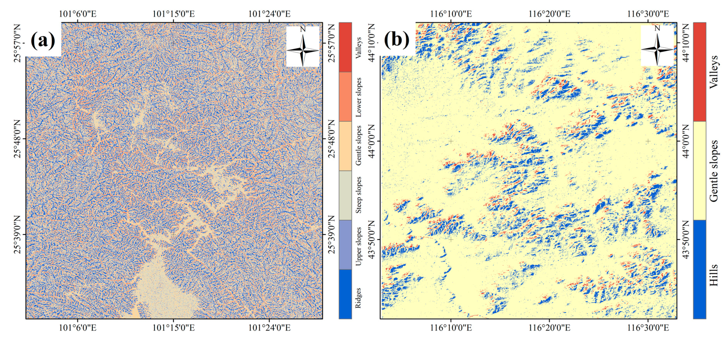
3.3. Slope Position Classifications

The topographic position index (TPI) [66] and the standard deviation of elevation (SDE) [67] can be used to divide the landscape into different slope locations. This article uses the SDE threshold value proposed by [66] to classify the landscape, as shown in Table 2. The value of the slope threshold (ST) is defined in agreement with [66], which is about one third of the steepest degree. After processing, the landscape is divided into 5 classes in mountainous areas—including lower slopes, gentle slopes, steep slopes, upper slopes, and ridges—while the low-relief area is divided into 3 classes: valleys, gentle slopes, and hills.
The calculation of TPI and SDE both require the definition of circular regions as neighborhoods. Furthermore, it is important to note that the TPI is very sensitive to the scale of the neighborhood, so the choice of scale is critical [68]. Appropriate scales can classify both small-scale features (such as valleys or fine ridge lines) and major topographic features (such as major valleys or mountains).

4. Results and Analysis
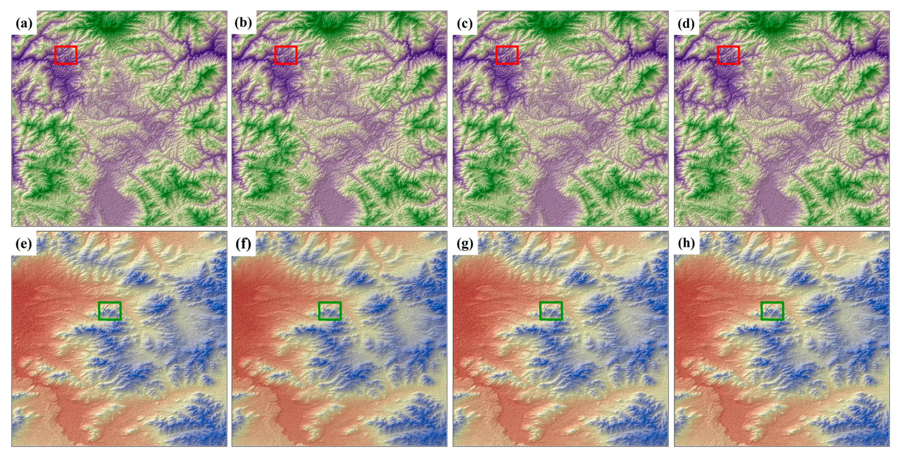
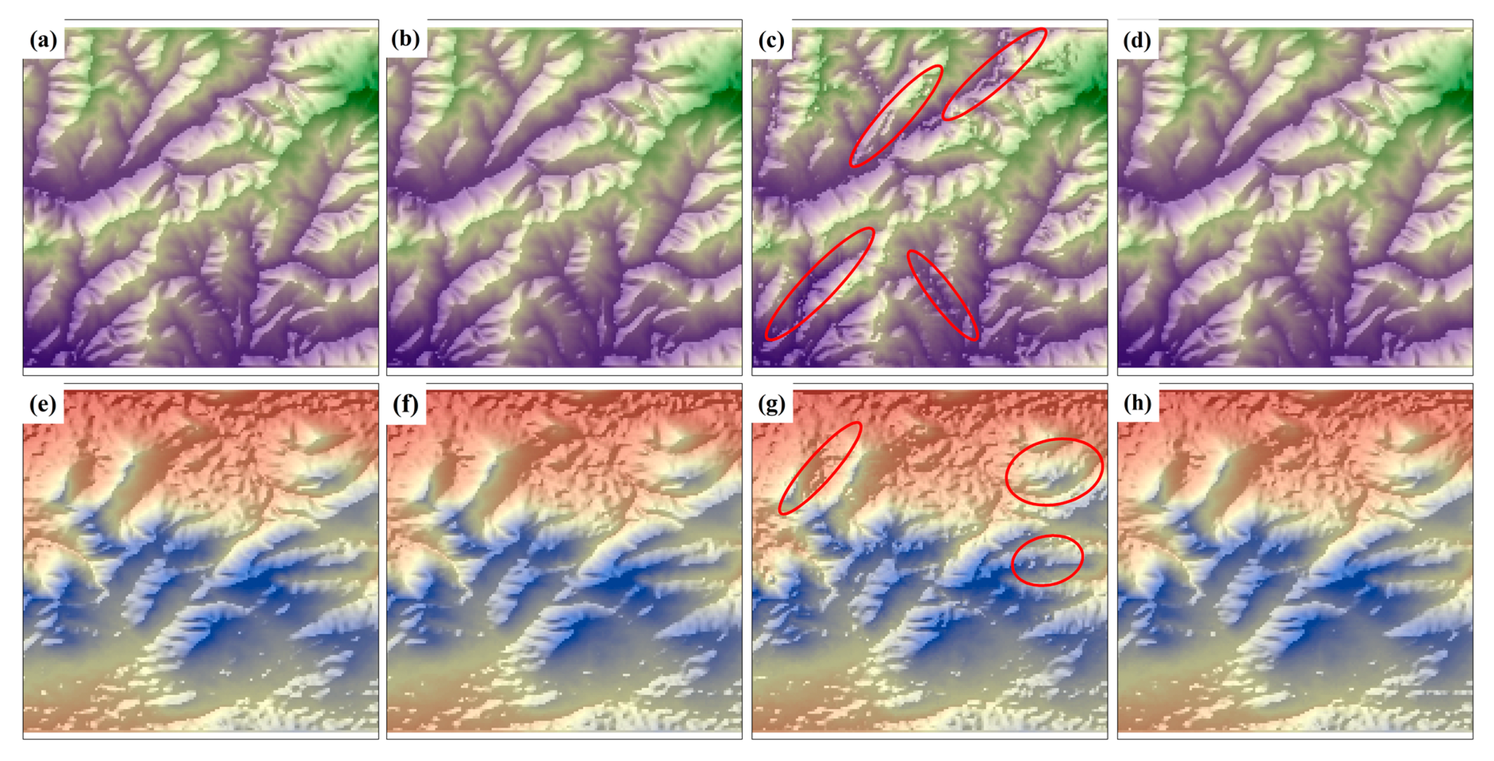
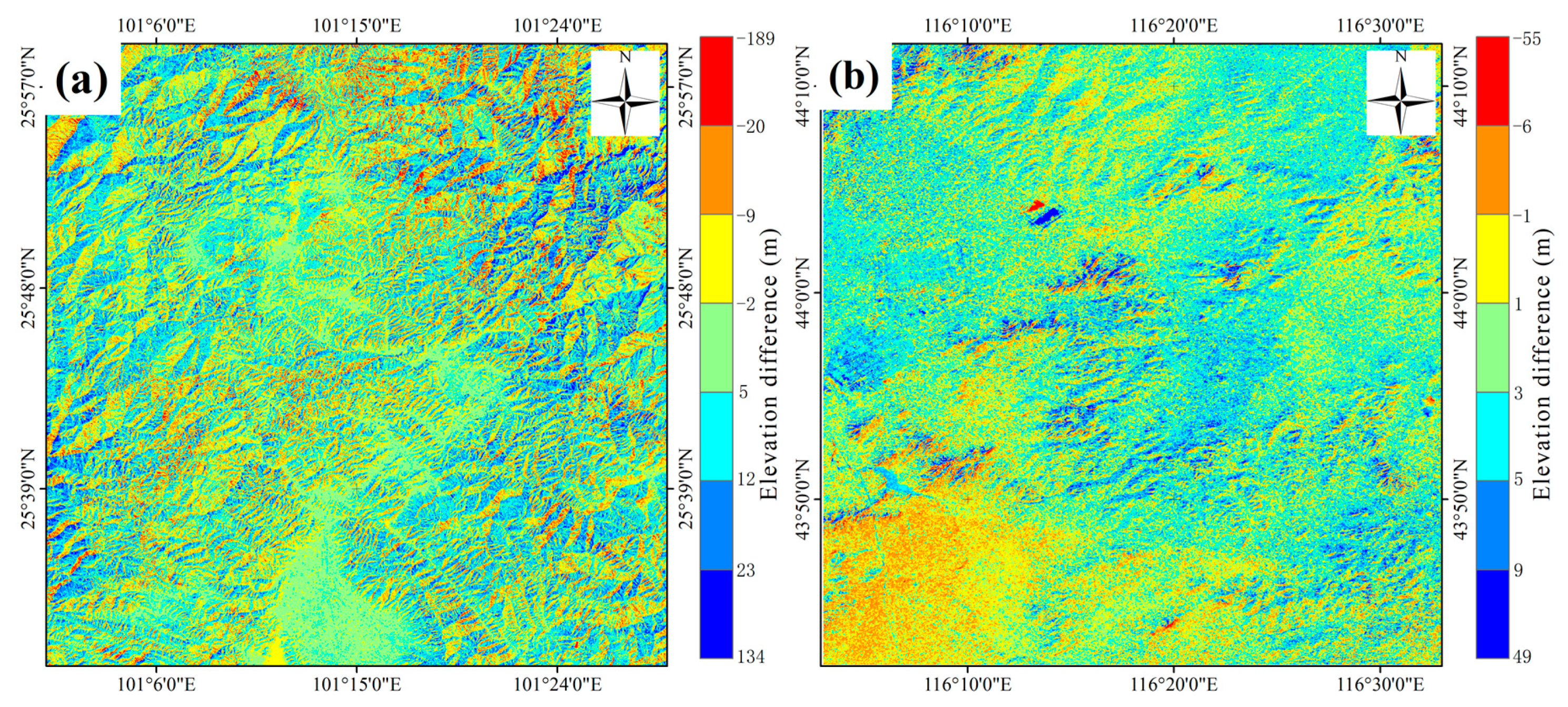
4.1. Fused DEM

The purpose of this paper is to obtain a fused DEM with higher accuracy, by fusing two kinds of DEMs. Three fusion methods are investigated in order to achieve this objective, i.e., the WT, BEMD, and N-AMD. The first step is to decompose both DEMs into different frequency components. It is known that the basis functions of the wavelet transform are not unique. Functions satisfying certain conditions can be used as the basis functions of the wavelet transform. DEM fusion using the WT is based on the wavelet coefficients at each scale, which are obtained by decomposition. The selection of a basis function affects the distribution of the wavelet coefficients to a certain extent, such that the quality of the basis function is directly related to the effectiveness of fusion. In addition, higher levels of decomposition generally achieve more effective fusion; however, such high levels of decomposition require greater computational capacity at the same time. Therefore, it is also important to choose the appropriate level of decomposition. To date, many experimental studies have been carried out to analyze the applicability of different basis functions and decomposition levels [69]. Referring to previous studies, typical orthogonal (Haar wavelet) and biorthogonal wavelet (Bior3.7 wavelet) basis functions are selected to decompose the DEMs into three levels.
The BEMD is a completely data-driven analysis method that does not require prior selection of the basis functions mentioned in Section 3.1.2. In BEMD, the Cauchy-type convergence condition is chosen as the stop condition of the screening process (SD = 0.3). Similar to BEMD, N-AMD is also a data-driven analysis method. To realize multi-scale decomposition of the DEM, the appropriate window size alone needs to be selected according to the desired level of decomposition. Three decomposition levels are compared for the BEMD and N-AMD, with the window sizes of N-AMD set to 21, 91, and 201.
Taking N-AMD as an example, Figure 6 shows the decomposition results of the AW3D30 at site A. The series of decomposition components, obtained by N-AMD, have different frequency values. The first-level component (Figure 6b) preserves most of the high-frequency information in the DEM, such as edge and texture details. The second-level component (Figure 6c) also keeps some information, but the details appear less clear than at the first level. The details of the third-level component (Figure 6d) are further reduced compared to those at the second level. The Residual (Figure 6e) retains most of the low-frequency component, which mainly contains the contour information and elevation distribution of the original DEM. The results are similar to N-AMD, using the WT and BEMD for DEM decomposition.
After decomposing the DEM into a series of components with different frequencies, the components are fused according to certain rules, and an inverse transformation applied to obtain the new DEM. The key to obtaining a high-quality fused DEM is using appropriate data fusion rules. The advantage of the above three methods of DEM fusion is that the DEMs are decomposed before the fusion rule is applied to the corresponding frequency components. Hence, analysis of the data is performed at multiple resolutions, such that the advantages of the individual original DEMs (for different frequency components) are comprehensively utilized in the fused DEM. The optimal solution is not always realized by averaging all of the corresponding elevation values to get the new height during fusion of the DEM [70]. Therefore, considering the actual physical meaning of the value in the DEM image—and how the fusion process differs from that of normal gray image fusion—the window-based fusion rule proposed in Section 3.2 is adopted, which can effectively reduce DEM errors in the fusion process due to outliers. The matching degree T is set to 0.6. The fused DEMs obtained by WT, BEMD, and N-AMD are listed in Figure 7. Owing to the limit of scale, the texture and detail information of the fused DEMs are not obvious in Figure 7. Hence, a small area is selected in each of sites A and B (defined by the red and green rectangles), as shown in Figure 8. It is apparent from the fusion results that the fusion quality varies quite significantly depending on the method used to obtain the fused DEM. The fused DEMs, obtained by the Bior3.7 wavelet, Haar wavelet, and N-AMD methods, correspond to Figure 8a,b–h in sites A and B, respectively. The texture and detail information is clear, and no significant difference can be observed. The fused DEMs, obtained by the BEMD method at sites A and B, correspond to Figure 8c,g, respectively. It is clear that both contain irregular patches in the ridge and valley regions (the red rectangles in Figure 8), which means that the detail information of the fused DEM is lost or distorted locally. Obviously, it does not meet the requirements for the application of the DEM. The reason is that the terrain of these two regions is irregular and complex. The irregularity of the extremum distribution causes improper fitting of the interpolation method in the BEMD. This results in patches appearing in the decomposition components, leading to local mutation of the fused DEMs.
In order to evaluate the quality of the fused DEM objectively, a quantitative metric is needed. The vertical accuracy of the DEM is the most important metric to evaluate the quality of the DEM. Since there is no high-precision DEM that can be used as a reference, the test set of the GLAH14 is used as reference data to understand the quality of the selected DEMs. After each of the datasets is pre-processed, the corresponding DEM elevation is extracted at each point of the test set. The difference in elevation is then calculated by subtracting the GLAH14 elevation from the corresponding DEM elevation. Subsequently, the mean error (ME) and root-mean-square-error (RMSE), which are two important quantitative metrics for evaluating the vertical accuracy of the DEM, are calculated. The results are shown in Table 3.
From Table 2, it is observed that the ME and RMSE of the AW3D30 and SRTM-1 in the low-relief grassland of site B are smaller than that of the mountainous area with a high density of vegetation of site A. This is due to the fact that the landscapes in site A are mainly mountainous with large surface fluctuations, shadows caused by the mountain, and vegetation artifacts, which lead to measurement errors in the DEM. The failure of optical technology to identify small terrain fluctuations in flat areas is responsible for the negative deviation of the ME of the AW3D30 at site B [71].
In addition, the difference between the ME of the fused DEM obtained by the three methods is not obvious, as a result of the fusion rule. The fused DEMs obtained by the Bior3.7 and Haar wavelet methods have similar error distribution characteristics, and both show a certain degree of improvement of the RMSE compared to the original DEM. The Haar wavelet method has better performance than the Bior3.7 wavelet method in both sites, which proves that different wavelet basis functions can obtain differing results. Consequently, better results can be obtained by selecting an appropriate wavelet basis function based on source data. Compared with the source DEM, the RMSE of the fused DEM obtained by BEMD in site B shows a certain level of improvement, but the improvement is not significant. Meanwhile, the RMSE of the fused DEM increases in site A, compared to the source DEM, which is consistent with the results from visual inspection. Therefore, it is concluded that the BEMD method is not suitable for DEM multi-scale decomposition and fusion of the multi-source DEM. N-AMD has better performance at both sites A and B compared to other methods. The RMSE of the fused DEM in site A is 7.696 m, which corresponds to a 19.3% and 29.6% increase in accuracy compared to the AW3D30 and SRTM-1, respectively. In site B, the RMSE is 1.902 m, and the accuracy is 15.5% and 27.4% higher than that of the AW3D30 and SRTM-1, respectively. Thus, the accuracy of the fused DEMs has been improved significantly using this method. Furthermore, the texture and detail information of the fused DEMs is clear and there is no mutation region. Exploring its causes, the N-AMD method is based on Taylor series expansion, and its fitting of the trend of the original signal is optimal or near optimal. Therefore, when using the N-AMD method to decompose AWAD30 and SRTM-1 respectively, the noise of two DEMs can be detected effectively and the consistency of trend signals can be ensured. Combining with the window-based fusion rule, the noise caused by weather conditions such as cloud cover, mist occlusion, and the abrupt change of surface roughness can be minimized. Hence, the fused DEM obtained by N-AMD, named DEMN, is chosen for further research.

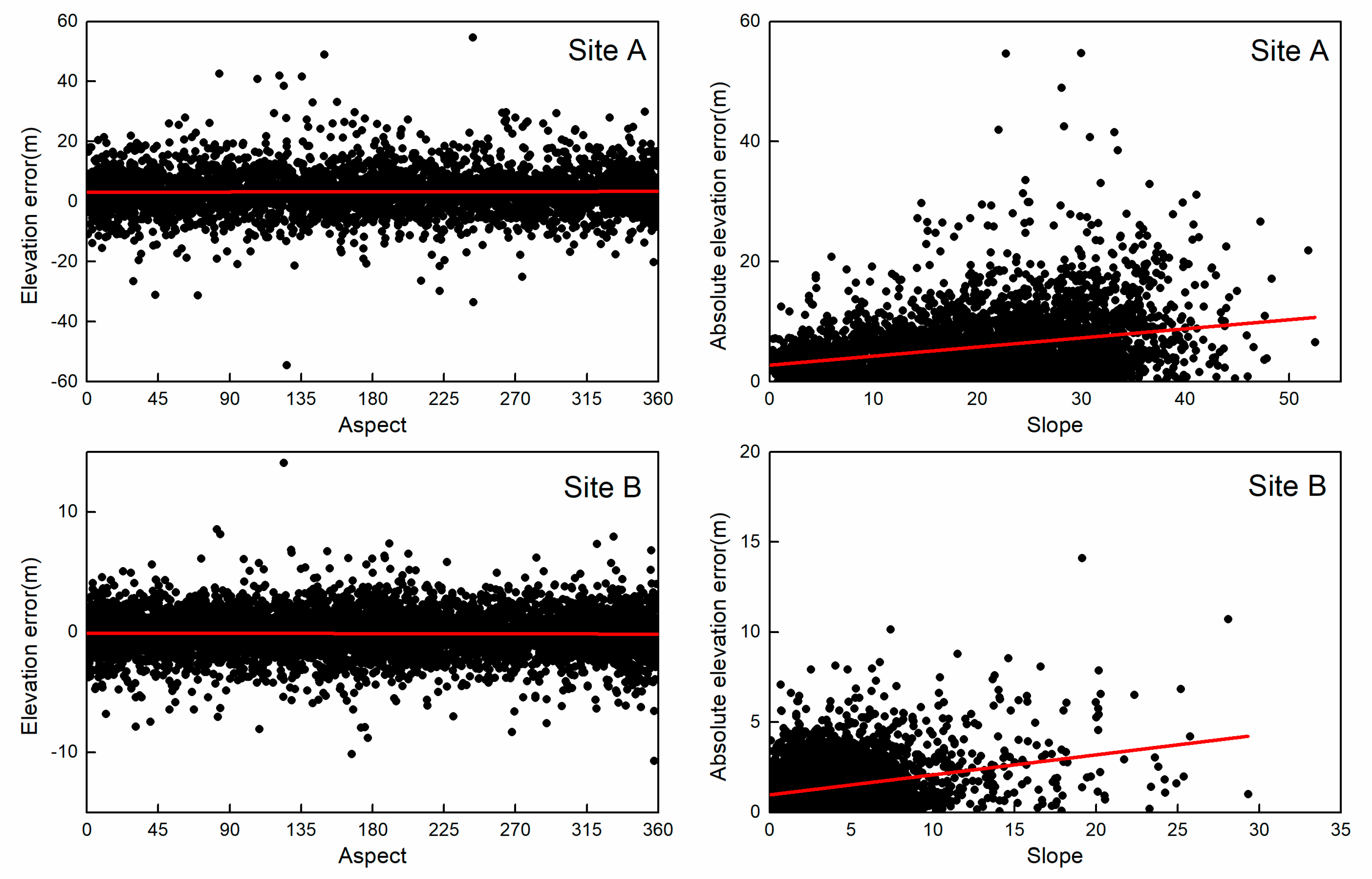
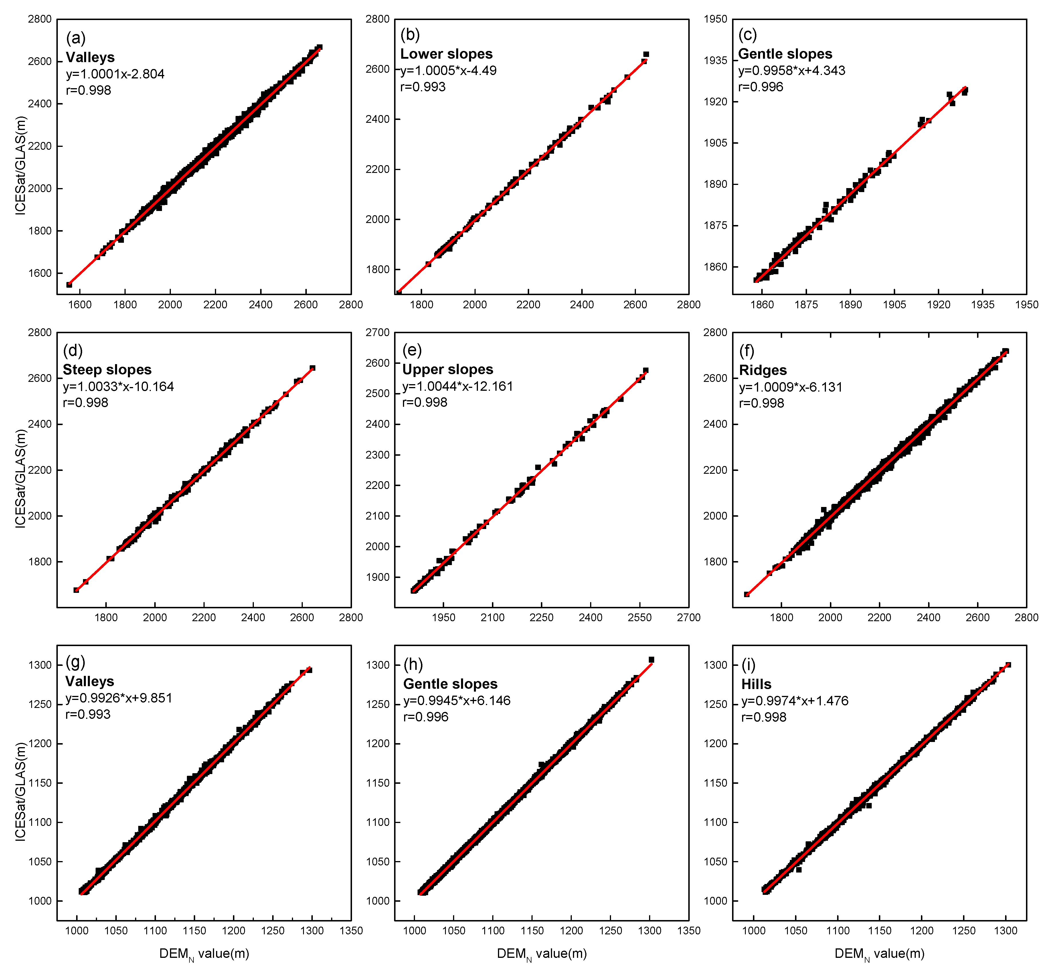
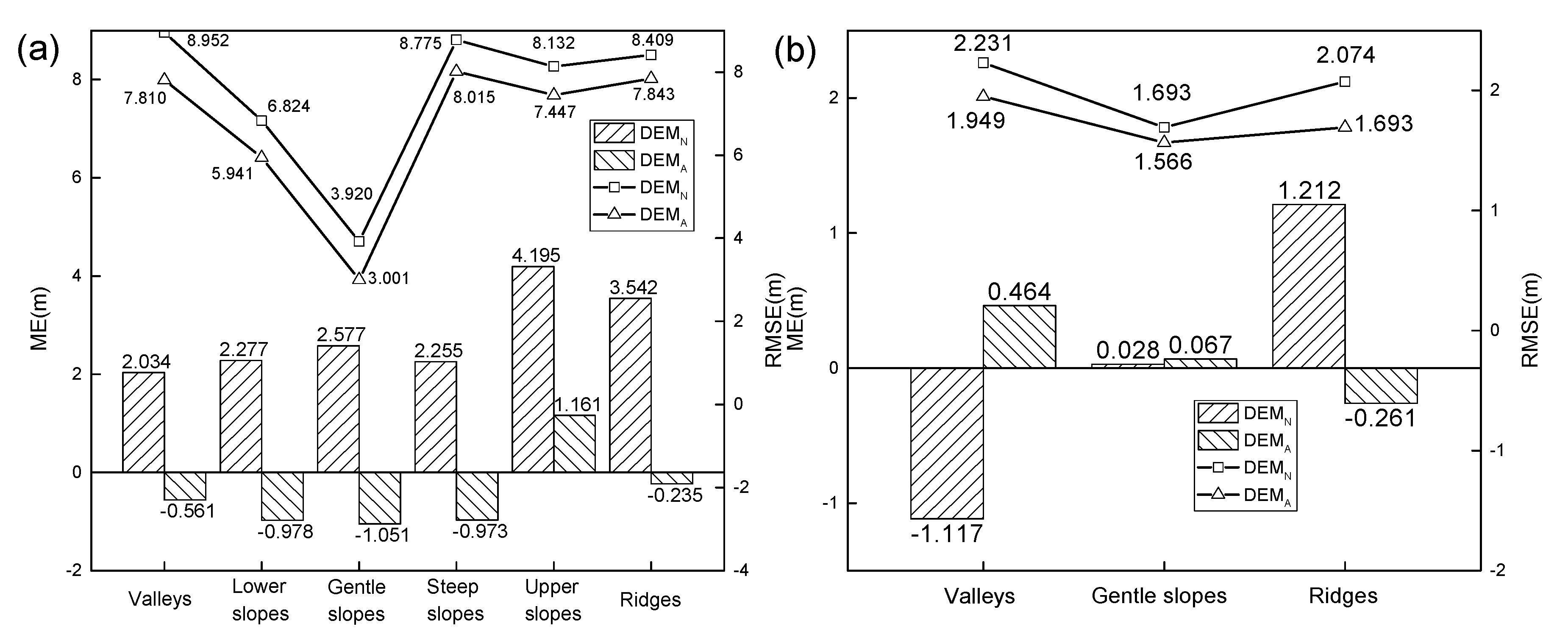
4.2. Fused DEM Errors for Different Slope Position Classifications

There is a significant correlation between elevation error and topographic factors (such as slope and aspect), which has been found in previous studies [16,43]. In order to examine the relationship between the elevation error of the fused DEM and terrain factors in the study areas, the SRTM-1 is subtracted from the AW3D30 to get the elevation difference (see Figure 9). Clearly, the area with an obvious difference between the two DEMs is also the area with a severe change of slope. Also, the fact that the value of the AW3D30 is lower than the SRTM-1 on one side of the ridge, and is opposite on the other side, indirectly proves that there is a significant correlation between elevation difference and terrain factors.
In this paper, the two DEMs produced by different techniques are decomposed by multi-scale analysis methods and then fused. Although this method can combine the advantages of source datasets to obtain a more accurate DEM, it still involves the fusion of corresponding pixels. Also, the sources of the DEMs have similar terrain factors (such as slope and aspect) in the same position, which means that the accuracy of the fused DEM is still affected by terrain factors. Therefore, the relationship between the DEM error and slope and aspect is studied further, in order to improve the accuracy of the fused DEM (based on DEMN).
Taking the GLAH14 test set as reference data, the relationship between the DEMN elevation error and slope and aspect is analyzed for sites A and B in Figure 10. The results show that the correlation between elevation error and aspect is not obvious for the two sites, and the whole distributing of the elevation error is uniform versus the aspect. However, the relationship between the absolute error of the elevation and slope at site A is similar to that at site B. Both of the absolute errors of elevation show an increasing trend with an increase of slope, especially at site A.
Considering the correlation between the DEMN elevation error and slope, the slope position classification method (mentioned in Section 3.3) is utilized to classify the terrain. It should be noted that the TPI is very sensitive to the scale of the neighborhood during this process. In order to select the best scale for each study area, the scale is gradually increased from 30 m to 720 m (with a step size of 30 m) for the two study sites. Depending on the classification results, scales of 120 m and 60 m are chosen at mountainous site A and low-relief site B, respectively. The classification results are shown in Figure 11.
The statistical measures of the elevation errors for different slope position classes are listed in Table 4. For study site A, the ME values are positive for all slope position classes, and RMSE values are largest in valleys and ridges, indicating that they have the lowest vertical accuracy of all classes. The next lowest values correspond to steep slopes and upper slopes. The precision of gentle slopes is the highest. At site B, the accuracies of valleys and ridges are the lowest. Similar to site A, the accuracy of the gentle slopes class is highest. It can be concluded that various slope position classes in sites A and B have differing error distributions. In this paper, a simple linear regression analysis is used to investigate the relationship between the DEMN and GLAH14 test set for different slope position classes at the two study sites (see Figure 12). The correlation coefficients of the fitted curves of the two regions are higher than 0.9, which demonstrates that the accuracy of the DEMN can be improved by using this simple linear regression model. However, it also varies with the class of the slope position. The improved DEM is generated by calibrating the DEMN with this regression model, called DEMA.
The ME and RMSE (taking the GLAH14 validation set as reference) of the DEMN and DEMA in different slope position classes are shown in Figure 13. The results show that the RMSE for different position classes has been reduced by varying degrees, and that the absolute value of the ME is reduced (except for gentle slopes) in site B. The change of the RMSE and ME after correction indicates that the slope position-based linear regression method is not effective in the flat area of grassland, but that it works well in other areas. With respect to the overall accuracy, the statistical error results are shown in Table 5. DEMw represents the result of linear correction for DEMN without slope position classification. It can be seen from the table that the linear correction effect on the DEMN of the whole area is not obvious due to the difference of errors distribution between various slope position classes. Meanwhile, we find that all of the errors of the DEMA are lower than those of the DEMN in site A (especially for the ME, which is reduced from 2.789 m to −0.241 m), indicating that the systematic error of the study region is reduced. Moreover, the RMSE has decreased by 16.0%. Compared with the DEMN, the ME of the DEMA is increased at site B. However, the RMSE has been reduced by 13.6%, which represents a significant improvement of vertical accuracy. The results show that the simple linear regression calibration method based on slope position classes is effective at improving the accuracy of the fused DEM.

5. Conclusions

In order to improve the accuracy of open source DEMs for applications in geographic and environmental fields, two sites in China are selected for research—a mountainous area and a low-relief area. In this paper, the AW3D30 is considered as an alternative dataset to the popular ASTER GDEM v2, in order to realize multi-scale fusion—using the WT, BEMD, and N-AMD methods—with SRTM-1 produced by INSAR technology, based on the fusion rule proposed in Section 3.2. Quantitative evaluation shows that BEMD, which is widely used in image fusion, is not suitable for multi-source DEM fusion products. Compared with existing open source DEMs, fused DEMs obtained by the WT and N-AMD methods have higher vertical accuracy, with the WT method showing worse performance than N-AMD. Due to space limitations, only two wavelet basis functions are selected to evaluate the performance of the WT. Hence, the effectiveness of the WT in multi-scale analysis of DEMs cannot be completely disregarded. Nonetheless, its applicability is inferior compared with N-AMD (which is a completely data-driven method that does not require any prior knowledge), since professional knowledge and a large number of experiments are required to select the appropriate basis functions. Consequentially, it is thought that the new N-AMD method has more potential in the application of fused DEMs. On the basis of analyzing the basic principles of DEM fusion, this paper explores the relationship between the error distribution of the fused DEM with terrain and proposes a slope position-based linear regression method to calibrate the DEMN in different slope position classes. Quantitative results show that the vertical accuracy of the fused DEM is further improved, which demonstrates the validity of this method. Future studies will focus on the calibration of the fused DEM using multiple linear regression analyses and refinement of the fusion rule. It is hoped that this paper provides a reference for future research that aims to obtain DEMs with higher accuracy using open source DEMs. The future work will try to simulate the error of two DEMs, thus creating simulated observations to which the different proposed algorithms can be applied. This would allow one to assess the performances of the different algorithms by comparing the results with an error-free reference digital elevation model.

Author Contributions

S.L. proposed research ideas; Y.T. and J.L. conceived and designed the experiments; Y.T. performed the experiments; Y.T. and S.L. analyzed the data; Z.B. and J.F. contributed reagents/materials/analysis tools; Y.T. wrote the paper. Z.B. and S.Z. offered guidance and supervision.

Funding

This research was funded by [National Key Research and Development Program] grant number [2016YFC0501107] and [Special Project of Science and Technology Basic Work of Ministry of Science and Technology of China] grant number [2014FY110800] And The APC was funded by [National Key Research and Development Program].

Acknowledgments

The research was supported by the projects funded by National Key Research and Development Program (No. 2016YFC0501107) and Special Project of Science and Technology Basic Work of Ministry of Science and Technology of China (Grant No. 2014FY110800).

Conflicts of Interest

The authors declare no conflict of interest.

References

  1. Yang, K.; Smith, L.C.; Chu, V.W.; Gleason, C.J.; Li, M. A Caution on the Use of Surface Digital Elevation Models to Simulate Supraglacial Hydrology of the Greenland Ice Sheet. IEEE J. Sel. Top. Appl. Earth Obs. Remote Sens. 2016, 8, 5212–5224. [Google Scholar] [CrossRef]
  2. Wechsler, S.P. Uncertainties associated with digital elevation models for hydrologic applications: A review. Hydrol. Earth Syst. Sci. 2007, 11, 1481–1500. [Google Scholar] [CrossRef]
  3. Yan, Y.; Tang, J.; Pilesjö, P. A combined algorithm for automated drainage network extraction from digital elevation models. Hydrol. Process. 2018, 32, 1322–1333. [Google Scholar] [CrossRef]
  4. Shukla, G.; Garg, R.D.; Srivastava, H.S.; Garg, P.K. Performance analysis of different predictive models for crop classification across an aridic to ustic area of Indian states. Geocarto Int. 2016, 33, 1–48. [Google Scholar] [CrossRef]
  5. Fu, P.; Rich, P. A geometric solar radiation model with applications in agriculture and forestry. Comput. Electron. Agric. 2002, 37, 25–35. [Google Scholar] [CrossRef]
  6. Chen, L.; Yang, X.; Chen, L.; Potter, R.; Li, Y. A state-impact-state methodology for assessing environmental impact in land use planning. Environ. Impact Assess. Rev. 2014, 46, 1–12. [Google Scholar] [CrossRef]
  7. Næsset, E.; Ørka, H.O.; Solberg, S.; Bollandsås, O.M.; Hansen, E.H.; Mauya, E.; Zahabu, E.; Malimbwi, R.; Chamuya, N.; Olsson, H. Mapping and estimating forest area and aboveground biomass in miombo woodlands in Tanzania using data from airborne laser scanning, TanDEM-X, RapidEye, and global forest maps: A comparison of estimated precision. Remote Sens. Environ. 2016, 175, 282–300. [Google Scholar] [CrossRef]
  8. Zhang, L.; Liu, S.; Sun, P.; Wang, T.; Wang, G.; Wang, L.; Zhang, X. Using DEM to predict Abies faxoniana and Quercus aquifolioides distributions in the upstream catchment basin of the Min River in southwest China. Ecol. Indic. 2016, 69, 91–99. [Google Scholar] [CrossRef]
  9. Carrara, A.; Bitelli, G.; Carla, R. Comparison of techniques for generating digital terrain models from contour lines. Int. J. Geogr. Inf. Syst. 1997, 11, 451–473. [Google Scholar] [CrossRef]
  10. Siart, C.; Bubenzer, O.; Eitel, B. Combining digital elevation data (SRTM/ASTER), high resolution satellite imagery (Quickbird) and GIS for geomorphological mapping: A multi-component case study on Mediterranean karst in Central Crete. Geomorphology 2009, 112, 106–121. [Google Scholar] [CrossRef]
  11. Kervyn, M.; Ernst, G.G.J.; Goossens, R.; Jacobs, P. Mapping volcano topography with remote sensing: ASTER vs. SRTM. Int. J. Remote Sens. 2008, 29, 6515–6538. [Google Scholar] [CrossRef]
  12. Malthus, T.J. Bio-Optical Modeling and Remote Sensing of Aquatic Macrophytes. In Bio-optical Modeling and Remote Sensing of Inland Waters; Mishra, D.R., Ogashawara, I., Gitelson, A., Eds.; Elsevier: Amsterdam, the Netherlands, 2017; pp. 263–308. [Google Scholar]
  13. Florinsky, I.V.; Skrypitsyna, T.N.; Luschikova, O.S. Comparative accuracy of the AW3D30 DSM, ASTER GDEM, and SRTM1 DEM: A case study on the Zaoksky testing ground, central European Russia. Remote Sens. Lett. 2018, 9, 706–714. [Google Scholar] [CrossRef]
  14. Ehlers, M.; Welch, R. Stereocorrelation of Landsat TM images. Photogramm. Eng. Remote Sens. 1987, 53, 1231–1237. [Google Scholar]
  15. Evans, D.L.; Apel, J.; Arvidson, R.; Bindschadler, R.; Carsey, F.; Dozier, J.; Jezek, K.; Kasischke, E.; Li, F.; Melack, J. Spaceborne Synthetic Aperture Radar: Current Status and Future Directions. A Report to the Committee on Earth Sciences; Space Studies Board, National Research Council: Washington, DC, USA, 1995; Volume 27, pp. 149–150. [Google Scholar]
  16. Pham, H.T.; Marshall, L.; Johnson, F.; Sharma, A. A method for combining SRTM DEM and ASTER GDEM2 to improve topography estimation in regions without reference data. Remote Sens. Environ. 2018, 210, 229–241. [Google Scholar] [CrossRef]
  17. Jarihani, A.A.; Callow, J.N.; McVicar, T.R.; Van Niel, T.G.; Larsen, J.R. Satellite-derived Digital Elevation Model (DEM) selection, preparation and correction for hydrodynamic modelling in large, low-gradient and data-sparse catchments. J. Hydrol. 2015, 524, 489–506. [Google Scholar] [CrossRef]
  18. Rawat, K.S.; Mishra, A.K.; Sehgal, V.K.; Ahmed, N.; Tripathi, V.K. Comparative evaluation of horizontal accuracy of elevations of selected ground control points from ASTER and SRTM DEM with respect to CARTOSAT-1 DEM: A case study of Shahjahanpur district, Uttar Pradesh, India. Geocarto Int. 2013, 28, 439–452. [Google Scholar] [CrossRef]
  19. Reinoso, J.F. An algorithm for automatically computing the horizontal shift between homologous contours from DTMs. ISPRS J. Photogramm. Remote Sens. 2011, 66, 272–286. [Google Scholar] [CrossRef]
  20. Reinoso, J.F.; León, C.; Mataix, J. Estimating horizontal displacement between DEMs by means of particle image velocimetry techniques. Remote Sens. 2016, 8. [Google Scholar] [CrossRef]
  21. Nuth, C.; Kääb, A. Co-registration and bias corrections of satellite elevation data sets for quantifying glacier thickness change. Cryosphere 2011, 5, 271–290. [Google Scholar] [CrossRef] [Green Version]
  22. O’Loughlin, F.E.; Paiva, R.C.D.; Durand, M.; Alsdorf, D.E.; Bates, P.D. A multi-sensor approach towards a global vegetation corrected SRTM DEM product. Remote Sens. Environ. 2016, 182, 49–59. [Google Scholar] [CrossRef]
  23. Baugh, C.A.; Bates, P.D.; Schumann, G.; Trigg, M.A. SRTM vegetation removal and hydrodynamic modeling accuracy. Water Resour. Res. 2013, 49, 5276–5289. [Google Scholar] [CrossRef] [Green Version]
  24. Reuter, H.I.; Nelson, A.; Jarvis, A. An evaluation of void-filling interpolation methods for SRTM data. Int. J. Geogr. Inf. Sci. 2007, 21, 983–1008. [Google Scholar] [CrossRef]
  25. Paredes-Hernández, C.U.; Tate, N.J.; Tansey, K.J.; Fisher, P.F.; Salinas-Castillo, W.E. Increasing the accuracy of digital elevation models by means of geostatistical conflation. In Proceedings of the 9th International Symposium on Spatial Accuracy Assessment in Natural Resources and Environmental Sciences, Leicester, UK, 20–23 July 2010. [Google Scholar]
  26. Felgueiras, C.A.; Ortiz, J.O.; Camargo, E.C.G. Application of geostatistical conflation techniques to improve the accuracy of digital elevation models. Proc. Braz. Symp. GeoInform. 2014, 149–155. [Google Scholar] [CrossRef]
  27. Kääb, A. Combination of SRTM3 and repeat ASTER data for deriving alpine glacier flow velocities in the Bhutan Himalaya. Remote Sens. Environ. 2005, 94, 463–474. [Google Scholar] [CrossRef]
  28. Fabris, M.; Baldi, P.; Anzidei, M.; Pesci, A.; Bortoluzzi, G.; Aliani, S. High resolution topographic model of Panarea Island by fusion of photogrammetric, lidar and bathymetric digital terrain models. Photogramm. Rec. 2010, 25, 382–401. [Google Scholar] [CrossRef]
  29. Podobnikar, T. Production of integrated digital terrain model from multiple datasets of different quality. Int. J. Geogr. Inf. Sci. 2005, 19, 69–89. [Google Scholar] [CrossRef]
  30. Schultz, H.; Riseman, E.M.; Stolle, F.R.; Woo, D.M. Error Detection and DEM Fusion Using Self-Consistency. In Proceedings of the Seventh IEEE International Conference on Computer Vision, Kerkyra, Greece, 20–27 September 1999. [Google Scholar]
  31. Honikel, M. Improvement of INSAR DEM accuracy using data and sensor fusion. In 1998 IEEE International Geoscience and Remote Sensing. Symposium Proceedings; IEEE: New York, NY, USA, 1998; Volume 5, pp. 2348–2350. [Google Scholar]
  32. Schindler, K.; Papasaika-Hanusch, H.; Schutz, S.; Baltsavias, E. Improving wide-area DEMs through data fusion-chances and limits. Proc. Photogramm. Week 2011, 11, 159–170. [Google Scholar]
  33. Karkee, M.; Steward, B.L.; Aziz, S.A. Improving quality of public domain digital elevation models through data fusion. Biosyst. Eng. 2008, 101, 293–305. [Google Scholar] [CrossRef]
  34. Tadono, T.; Ishida, H.; Oda, F.; Naito, S.; Minakawa, K.; Iwamoto, H. Precise Global DEM Generation by ALOS PRISM. ISPRS Ann. Photogramm. Remote Sens. Spat. Inf. Sci. 2014, ii-4, 71–76. [Google Scholar] [CrossRef]
  35. JAXA ALOS Global Digital Surface Model “ALOS World 3D-30m (AW3D30)”. Available online: http://www.eorc.jaxa.jp/ALOS/en/aw3d30/ (accessed on 20 April 2018).
  36. Santillan, J.R.; Makinanosantillan, M. Vertical Accuracy Assessment of 30-M Resolution Alos, Aster, and Srtm Global Dems Over Northeastern Mindanao, Philippines. ISPRS-Int. Arch. Photogramm. Remote Sens. Spat. Inf. Sci. 2016, XLI-B4, 149–156. [Google Scholar] [CrossRef]
  37. Gao, J. Resolution and accuracy of terrain representation by grid DEMs at a micro-scale. Int. J. Geogr. Inf. Syst. 1997, 11, 199–212. [Google Scholar] [CrossRef]
  38. Honikel, M. Fusion of optical and radar digital elevation models in the spatial frequency domain. In Proceedings of the Second Int. Workshop on Retreieval of Bio- and Geophysical Parameters from SAR Data for Land Application, Noordwijwk, The Newerlands, October 1998; pp. 537–543. [Google Scholar]
  39. Hu, J.; Gao, J.; Wang, X. Multifractal analysis of sunspot time series: The effects of the 11-year cycle and Fourier truncation. J. Stat. Mech. Theory Exp. 2009, P02066, 57–94. [Google Scholar] [CrossRef]
  40. Tung, W.W.; Gao, J.; Hu, J.; Yang, L. Detecting chaos in heavy-noise environments. Phys. Rev. E 2011, 83, 46210. [Google Scholar] [CrossRef] [PubMed]
  41. Gao, J.; Sultan, H.; Hu, J.; Tung, W.W. Denoising Nonlinear Time Series by Adaptive Filtering and Wavelet Shrinkage: A Comparison. IEEE Signal Process. Lett. 2009, 17, 237–240. [Google Scholar]
  42. Yang, X.; Long, L.I.; Chen, L.; Chen, L.; Shen, Z. Improving ASTER GDEM accuracy using land use-based linear regression methods: A case study of Lianyungang, East China. Int. J. Geo-Inf. 2018, 7, 145. [Google Scholar] [CrossRef]
  43. Zyl, J.J. Van The Shuttle Radar Topography Mission (SRTM): A breakthrough in remote sensing of topography. Acta Astronaut. 2001, 48, 559–565. [Google Scholar]
  44. Gamache, M.; Guild, A.M. Free and Low Cost Datasets for International Mountain Cartography. In Proceedings of the 4th ICA Mountain Cartography Workshop, Catalonia, Spain, 30 September–2 October 2004. [Google Scholar]
  45. Takaku, J.; Tadono, T.; Tsutsui, K.; Ichikawa, M. Validation of “AW3D” Global Dsm Generated from Alos Prism. Isprs Ann. Photogramm. Remote Sens. Spat. Inf. 2016, III-4, 25–31. [Google Scholar] [CrossRef]
  46. Satgé, F.; Bonnet, M.P.; Timouk, F.; Calmant, S.; Pillco, R.; Molina, J.; Lavado-Casimiro, W.; Arsen, A.; Crétaux, J.F.; Garnier, J. Accuracy assessment of SRTM v4 and ASTER GDEM v2 over the Altiplano watershed using ICESat/GLAS data. Int. J. Remote Sens. 2015, 36, 465–488. [Google Scholar] [CrossRef]
  47. Abshire, J.B.; Sun, X.; Riris, H.; Sirota, J.M.; Mcgarry, J.F.; Palm, S.; Yi, D.; Liiva, P. Geoscience Laser Altimeter System (GLAS) on the ICESat Mission: On-orbit measurement performance. Geophys. Res. Lett. 2003, 32. [Google Scholar] [CrossRef]
  48. Shuman, C.A.; Zwally, H.J.; Schutz, B.E.; Brenner, A.C.; Dimarzio, J.P.; Suchdeo, V.P.; Fricker, H.A. ICESat Antarctic elevation data: Preliminary precision and accuracy assessment. Geophys. Res. Lett. 2015, 33, 359–377. [Google Scholar] [CrossRef]
  49. Fricker, H.A.; Borsa, A.; Minster, B.; Carabajal, C.; Quinn, K.; Bills, B. Assessment of ICESat performance at the salar de Uyuni, Bolivia. Geophys. Res. Lett. 2005, 32. [Google Scholar] [CrossRef] [Green Version]
  50. Huber, M.; Wessel, B.; Kosmann, D.; Felbier, A.; Schwieger, V.; Habermeyer, M.; Wendleder, A.; Roth, A. Ensuring Globally the TanDEM-X Height Accuracy: Analysis of the Reference Data Sets ICESat, SRTM and KGPS-Tracks. In Proceedings of the IEEE International Geoscience and Remote Sensing Symposium (IGARSS ’09), Cape Town, South Africa, 12–17 June 2009; pp. 769–772. [Google Scholar]
  51. Arefi, H.; Reinartz, P. Accuracy Enhancement of ASTER Global Digital Elevation Models Using ICESat Data. Remote Sens. 2011, 3, 1323–1343. [Google Scholar] [CrossRef] [Green Version]
  52. Van Niel, T.G.; Mcvicar, T.R.; Li, L.T.; Gallant, J.C.; Yang, Q.K. The impact of misregistration on SRTM and DEM image differences. Remote Sens. Environ. 2008, 112, 2430–2442. [Google Scholar] [CrossRef]
  53. Gallant, J.C.; Read, A.M.; Dowling, T.I. Removal of Tree Offsets from Srtm and Other Digital Surface Models. ISPRS—Int. Arch. Photogramm. Remote Sens. Spat. Inf. Sci. 2012, XXXIX-B4, 275–280. [Google Scholar] [CrossRef]
  54. Yue, L.; Shen, H.; Zhang, L.; Zheng, X.; Zhang, F.; Yuan, Q. High-quality seamless DEM generation blending SRTM-1, ASTER GDEM v2 and ICESat/GLAS observations. Isprs J. Photogramm. Remote Sens. 2017, 123, 20–34. [Google Scholar] [CrossRef]
  55. Baghdadi, N.; Lemarquand, N.; Abdallah, H.; Bailly, J.S. The Relevance of GLAS/ICESat Elevation Data for the Monitoring of River Networks. Remote Sens. 2011, 3, 708–720. [Google Scholar] [CrossRef] [Green Version]
  56. Aghajani, A.; Kazemzadeh, R.; Ebrahimi, A. A novel hybrid approach for predicting wind farm power production based on wavelet transform, hybrid neural networks and imperialist competitive algorithm. Energy Convers. Manag. 2016, 121, 232–240. [Google Scholar] [CrossRef]
  57. Belayneh, A.; Adamowski, J.; Khalil, B.; Quilty, J. Coupling machine learning methods with wavelet transforms and the bootstrap and boosting ensemble approaches for drought prediction. Atmos. Res. 2016, 172–173, 37–47. [Google Scholar] [CrossRef]
  58. Yu, M.; Guo, H.; Zou, C. Application of wavelet analysis to GPS deformation monitoring. In Proceedings of the Position, Location, and Navigation Symposium, Coronado, CA, USA, 24–27 April 2006; pp. 670–676. [Google Scholar]
  59. Mallat, S. A Wavelet Tour of Signal Processing; Academic Press: Cambridge, MA, USA, 1998. [Google Scholar]
  60. Daubechies, I.; Heil, C. Ten Lectures on Wavelets. Comput. Phys. 1998, 6, 1671. [Google Scholar]
  61. Huang, N.E.; Shen, Z.; Long, S.R.; Wu, M.C.; Shih, H.H.; Zheng, Q.; Yen, N.C.; Chi, C.T.; Liu, H.H. The Empirical Mode Decomposition and the Hilbert Spectrum for Nonlinear and Non-Stationary Time Series Analysis. Proc. Math. Phys. Eng. Sci. 1998, 454, 903–995. [Google Scholar] [CrossRef]
  62. Nunes, J.C.; Bouaoune, Y.; Delechelle, E.; Niang, O.; Bunel, P. Image analysis by bidimensional empirical mode decomposition. Image Vis. Comput. 2003, 21, 1019–1026. [Google Scholar] [CrossRef]
  63. Equis, S.; Jacquot, P. The empirical mode decomposition: A must-have tool in speckle interferometry? Opt. Express 2009, 17, 611–623. [Google Scholar] [CrossRef] [PubMed]
  64. Chen, Y.; Wang, L.; Sun, Z.; Jiang, Y.; Zhai, G. Fusion of color microscopic images based on bidimensional empirical mode decomposition. Opt. Express 2010, 18, 21757–21769. [Google Scholar] [CrossRef] [PubMed]
  65. Burt, P.J.; Kolczynski, R.J. Enhanced image capture through fusion. In Proceedings of the 1993 (4th) International Conference on Computer Vision, Berlin, Germany, 11–14 May 1993; pp. 173–182. [Google Scholar] [Green Version]
  66. Weiss, A. Topographic Position and Landforms Analysis. In Proceedings of the ESRI User Conference, San Diego, CA, USA, 9–13 July 2001. [Google Scholar]
  67. Wilson, J.P.; Gallant, J.C. Terrain Analysis: Principles and Applications; John Wiley & Sons: New York, NY, USA, 2000. [Google Scholar]
  68. Strebeck, J.; Kroenung, G.; Grohman, G. Filling SRTM Voids: The Delta Surface Fill Method. Photogramm. Eng. Remote Sens. 2006, 72, 213–216. [Google Scholar]
  69. Gong, J.Z.; Liu, Y.S.; Xia, B.C.; Chen, J.F. Effect of Wavelet Basis and Decomposition Levels on Performance of Fusion Images from Remotely Sensed Data. Geogr. Geo-Inf. Sci. 2010, 26, 6–186. [Google Scholar]
  70. Hoja, D.; D’Angelo, P. Analysis of DEM combination methods using high resolution optical stereo imagery and interferometric SAR data. In Proceedings of the ISPRS HighResolution Earth Imaging for Geospatial Information, Hannover, Germany, 2–5 June 2009. [Google Scholar]
  71. Forkuor, G.; Maathuis, B. Comparison of SRTM and ASTER Derived Digital Elevation Models over Two Regions in Ghana–Implications for Hydrological and Environmental Modeling. In Studies on Environmental and Applied Geomorphology; InTech: Rijeka, Croatia, 2012; pp. 219–240. [Google Scholar]
Figure 1. Locations of (a) the mountainous site and (b) the low-relief site.
Remotesensing 10 01861 g001
Figure 2. Distribution of the GLAH14 points (red) in (a) the mountainous site, and (b) the low-relief site.
Remotesensing 10 01861 g002
Figure 3. Schematic flowchart of the multi-scale fusion of the SRTM-1 and AW3D30.
Remotesensing 10 01861 g003
Figure 4. Schematic of three level wavelet decomposition of the SRTM-1.
Remotesensing 10 01861 g004
Figure 5. Schematic of data decomposition using N-AMD: (a) three 2nd order polynomial fitted lines, (b) the fitted trend with window sizes of 21 and 121, and (c) different frequency components of the original data using various window sizes, where Residue is the fitted trend of original data with a window size of 121, level2 is the fitted trend of (original data − Residue) with a window size of 21, and level1 is the remaining part that satisfies the relationship: original data = (level)1 + (level)2 + (Residue).
Remotesensing 10 01861 g005
Figure 6. Schematic of N-AMD decomposition, including: (a) the original AW3D30, (b) the first-level component, (c) the second-level component, (d) the third-level component, and (e) the Residue.
Remotesensing 10 01861 g006
Figure 7. The fused DEMs obtained using the Bior3.7 wavelet, Haar wavelet, BEMD, and N-AMD methods at (ad) site A and (eh) site B. The red and green rectangles are the areas selected in sites A and B that are enlarged in Figure 8.
Remotesensing 10 01861 g007
Figure 8. Enlarged images of the fused DEMs obtained using the Bior3.7 wavelet, Haar wavelet, BEMD, and N-AMD methods at (ad) site A and (eh) site B. The red shapes indicate irregular patches.
Remotesensing 10 01861 g008
Figure 9. Illustration of the elevation difference between the AW3D30 and SRTM-1 in (a) the mountainous area, and (b) the low-relief area.
Remotesensing 10 01861 g009
Figure 10. Relationship between the DEMN elevation error and slope and aspect.
Remotesensing 10 01861 g010
Figure 11. The slope position classes in (a) the mountainous site, and (b) the low-relief site.
Remotesensing 10 01861 g011
Figure 12. Plots of the DEMN against the GLAH14 in different slope position classes at (af) site A, and (gi) site B.
Remotesensing 10 01861 g012
Figure 13. The ME and RMSE of the DEMN and DEMA in different slope position classes in (a) site A and (b) site B.
Remotesensing 10 01861 g013
Table 1. The basic parameters of the the 1-arc-second Shuttle Radar Topography Mission Global digital elevation model (SRTM-1 DEM), the Advanced Land Observing Satellite World 3D—30 m digital surface model (AW3D30 DSM), and the Ice Cloud and Land Elevation Satellite (ICESat) global land surface altimetry product.
SRTM-1AW3D30ICESat Product
Geographic datumWGS84GRS80Topex/Poseion
Elevation datumEGM96EGM96Topex/Poseion
Resolution1′′ (30 m)1′′ (30 m)70 m
Horizontal accuracy20 m5 m6 m
Vertical accuracy16 m5 m0.15 m
Table 2. Thresholds of standard deviation of elevation (SDE) corresponding to different slope positions.
Slope PositionSDE ThresholdsSlope PositionSDE Thresholds
Mountainous Area(A)Low-Relief Area(B)
ValleysTPI ≤−1.0 SDEValleysTPI > +1.0 SDE
Lower slopes−1.0 SDE < TPI ≤ −0.5 SDEGentle slopes−1.0 SDE < TPI ≤ +1.0 SDE
Gentle slopes−0.5 SDE < TPI ≤ +0.5SDE,
Slope ≤ ST
Hills+1.0 SDE < TPI
Steep slopes−0.5 SDE < TPI ≤ +0.5SDE,
Slope > ST
Upper slopes+0.5SDE < TPI ≤ +1.0 SDE
RidgesTPI > +1.0 SDE
Table 3. Accuracy statistics of original DEMs and fused DEMs.
DEMsSite ASite B
ME (m)RMSE (m)ME (m)RMSE (m)
AW3D304.59.535−1.2962.252
SRTM-12.12510.9281.0682.619
Bior3.7 wavelet3.2359.08−0.2242.07
Haar wavelet3.3268.916−0.1341.999
BEMD3.23510.949−0.1522.191
N-AMD3.1737.696−0.1141.902
Table 4. Statistical measures of elevation errors for different slope position classes.
ErrorSite ASite B
ValleysLower SlopesGentle SlopesSteep SlopesUpper SlopesRidgesValleysGentle SlopesHills
ME(m)2.2073.3453.5343.0932.9443.749−1.634−0.0531.364
RMSE(m)9.1416.1173.7358.3317.4979.1832.7181.3572.697
Table 5. Performance of the adjusted DEM in comparison with the DEMN at study sites A and B.
SitesGLAH14DEMNDEMADEMw
ME (m)RMSE (m)ME (m)RMSE (m)ME (m)RMSE (m)
A17122.7897.947−0.2416.6722.5447.682
B21360.0161.9560.0381.690.0721.921

