Assessing Hydrological Modelling Driven by Different Precipitation Datasets via the SMAP Soil Moisture Product and Gauged Streamflow Data

1
State Key Laboratory of Pollution Control and Resource Reuse, School of the Environment, Nanjing University, Nanjing 210093, China
2
Key Laboratory of Digital Earth Science, Institute of Remote Sensing and Digital Earth, Chinese Academy of Sciences, Beijing 100094, China
3
Yellow River Conservancy Commission of the Ministry of Water Resources, Zhengzhou 210046, China
*
Author to whom correspondence should be addressed.
Remote Sens. 2018, 10(12), 1872; https://doi.org/10.3390/rs10121872
Submission received: 18 October 2018
/
Revised: 15 November 2018
/
Accepted: 21 November 2018
/
Published: 23 November 2018
(This article belongs to the Special Issue Assimilation of Remote Sensing Data into Earth System Models)
Abstract
:To compare the effectivenesses of different precipitation datasets on hydrological modelling, five precipitation datasets derived from various approaches were used to simulate a two-week runoff process after a heavy rainfall event in the Wangjiaba (WJB) watershed, which covers an area of 30,000 km2 in eastern China. The five precipitation datasets contained one traditional in situ observation, two satellite products, and two predictions obtained from the Numerical Weather Prediction (NWP) models. They were the station observations collected from the China Meteorological Administration (CMA), the Integrated Multi-satellite Retrievals for Global Precipitation Measurement (GPM IMERG), the merged data of the Climate Prediction Center Morphing (merged CMORPH), and the outputs of the Weather Research and Forecasting (WRF) model and the WRF four-dimensional variational (4D-Var) data assimilation system, respectively. Apart from the outlet discharge, the simulated soil moisture was also assessed via the Soil Moisture Active Passive (SMAP) product. These investigations suggested that (1) all the five precipitation datasets could yield reasonable simulations of the studied rainfall-runoff process. The Nash-Sutcliffe coefficients reached the highest value (0.658) with the in situ CMA precipitation and the lowest value (0.464) with the WRF-predicted precipitation. (2) The traditional in situ observation were still the most reliable precipitation data to simulate the study case, whereas the two NWP-predicted precipitation datasets performed the worst. Nevertheless, the NWP-predicted precipitation is irreplaceable in hydrological modelling because of its fine spatiotemporal resolutions and ability to forecast precipitation in the future. (3) Gauge correction and 4D-Var data assimilation had positive impacts on improving the accuracies of the merged CMORPH and the WRF 4D-Var prediction, respectively, but the effectiveness of the latter on the rainfall-runoff simulation was mainly weakened by the poor quality of the GPM IMERG used in the study case. This study provides a reference for the applications of different precipitation datasets, including in situ observations, remote sensing estimations and NWP simulations, in hydrological modelling.
1. Introduction
Numerical simulation of the rainfall-runoff process is an important way to research water cycle, flood monitoring, water resource management and environmental conservation [1,2,3,4,5]. The performance of a rainfall-runoff simulation differs from the applied hydrological model, calibrated parameters and input data [6,7,8,9]. Because of different theories of runoff generation and routing, different considerations for spatial variation of the underlying surface, and different scheme combinations, diverse hydrological models lead to different simulation results [10,11,12]. For a specific study area, when the applied hydrological model, required parameters, and other input data are fixed, precipitation is the most important datum that affects hydrological modelling, because its accuracy will dominantly influence the subsequent calculation qualities of net precipitation, soil moisture variation, runoff generation, and runoff routing, then finally determine the success of the rainfall-runoff simulation [13,14,15,16,17].
Currently, there are three mainstream ways to obtain precipitation data. One method is the use of traditional in situ observation [18]. This type of precipitation data is measured using the equipments set in precipitation stations, meteorological stations, or automatic weather stations, which are managed by different departments. The in situ observed precipitation is generally recognized as the most accurate datum that represents the true value [19,20]. However, its application in hydrology is limited by its poor point-to-area representativeness, incomplete opening and sparse station network in developing areas [21,22]. The second method is remote sensing estimation. This category of precipitation data emerged as the remote sensing techniques of visible, infrared and microwaves were developed. Commonly used satellite precipitation products contain the Global Precipitation Climatology Project (GPCP) [23], the Climate Prediction Center Morphing Technique (CMORPH) [24], the Tropical Rainfall Measuring Mission (TRMM) [25] and its successor, the Global Precipitation Measurement (GPM) [26]. These products not only cover a nearly global area but also are freely available to the public, and their spatiotemporal resolutions are becoming finer. Moreover, there are corresponding upgraded products after post-processing [27]. Nevertheless, the remotely sensed precipitation still falls short in terms of showing the consecutiveness of precipitation and detecting extreme events at high latitudes [28]. The third method is obtaining precipitation from a numerical weather prediction (NWP) model. Because this atmospheric model is built on precise physical governing equations, an NWP model can describe the inherent dynamics of precipitation, thus present nearly the entire precipitation process with specific atmospheric reanalysis data [29,30,31]. However, due to the incompleteness of initial and boundary conditions provided by reanalysis data, uncertainties are unavoidably included in the NWP outputs when solving the physical equations with approximations [32,33]. When applied in hydrological modelling, the poor precipitation prediction of an NWP model and the scale mismatch between it and a hydrological model are two primary problems [34,35,36]. To improve the accuracy of the NWP-predicted precipitation, various methods of data assimilation have been used to enhance the initial and lateral boundary conditions of an NWP model [37,38,39,40,41]. The generally used NWP models include the National Meteorological Center (NMC) forecast model [42], the next-generation Weather Research and Forecasting (WRF) model [43], the operational Japan Meteorological Agency (JMA) mesoscale model [44] and the European Centre for Medium-Range Weather Forecasts (ECMWF) [45].
These three methods of collecting precipitation data have been widely used in hydrological modelling [1,46,47,48,49,50,51,52,53,54,55]. Many studies have been conducted to investigate the utilities of remote sensing estimations and the NWP simulations in hydrological modelling. For example, Wu et al. [48] evaluated the performances of nine existing precipitation products, including TRMM, CMORPH, and NLDAS-2 (Phase 2 of the North American Land Data Assimilation System), in the DRIVE model system for simulating a series of flood in Iowa. Essou et al. [1] applied global atmospheric reanalysis data to drive the lumped conceptual hydrological model HSAMI over 370 American watersheds. Liechti et al. [52] used TRMM 3B42 to drive the hydraulic-hydrologic model over the African Zambezi basin. Rasmussen et al. [49] investigated the spatial-scale characteristics of the precipitation predicted by the WRF model and its applications in hydrological modelling; they concluded that the RCM predictions had larger predictive certainty at a larger scale than at a smaller scale. Lin et al. [51] used the precipitation data generated by the Canadian atmospheric Mesoscale Compressible Community Model (MC2) to drive the Chinese Xin’anjiang hydrological model and simulated a series of flood events in the Huaihe River basin at a 5-km resolution. All of these investigations demonstrated the potential of the indirectly measured precipitation to be used in hydrological modelling. Nevertheless, there are still limited studies concerning the different effectivenesses of different precipitation datasets in hydrological modelling. Therefore, five types of precipitation datasets, incorporating one traditional in situ station observation, two satellite precipitation products, and two NWP predictions, were collected, evaluated and applied in hydrological modelling in this study. Moreover, to avoid the uncertainties caused by scale mismatch between the NWP and hydrological models [49], a 1-km resolution, which the applied NWP and hydrological models could realize, was employed in the simulations. Furthermore, as soil moisture is a crucial intermediate variable in hydrological modelling that affects water exchange, evapotranspiration estimation, runoff generation and model simulation [56,57,58,59,60,61], hydrologists have extended their attention to assess and improve the accuracy of soil moisture simulation to ensure the reasonability of hydrological simulation [62,63,64,65,66,67,68,69]. Therefore, we assessed the performances of the hydrological modelling driven by different precipitation datasets via not only outlet discharge but also soil moisture.
This manuscript is structured as follows: Section 2 introduces the study area, study period and study data. Section 3 introduces the experimental design and evaluation metrics. Section 4 shows 1-km grid data obtained from different precipitation datasets, the simulated soil moisture and outlet discharges. Section 5 presents the evaluations of different precipitation datasets, the simulated soil moisture and outlet discharges. Finally, the conclusions are drawn in Section 6.
2. Data
2.1. Study Area and Study Period
2.1.1. Study Area
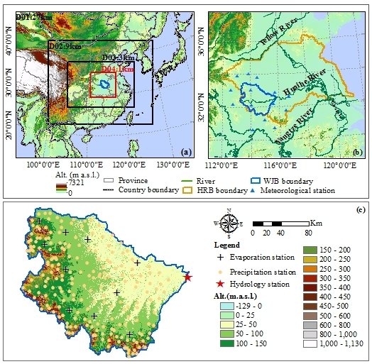
As the NWP predictions generally have larger predictive certainty at a larger scale than at a smaller scale [35,49], a large-scale watershed covering an area of 30,630 km2, namely, Wangjiaba (WJB) was selected as the study area. The WJB watershed is located between 113.3°–115.8°E and 31.5°–33.4°N (Figure 1b); it is a sub-basin of the Huaihe River basin (HRB), which is one of the seven major river basins in China and lays between the Yellow and Yangtze rivers. This region has important political and economic functions because it has the highest population density in China and has 17% of the country’s cultivated land [51]. The WJB watershed belongs to the warm temperate and semi-humid monsoon climate. Its northern region is characterized by hot and wet summers and cold and dry winters because it is primarily controlled by the monsoon climate at mid-latitudes, while its southern part has hot and wet summers and mild and dry winters because it is dominated by a subtropical monsoon climate [70]. The regional elevation in this watershed decreases from the west to the east. In the west, there are foothills and mountains, and the highest altitude is 1130 m above sea level (m.a.s.l.). The middle and eastern parts are vast plains. In this watershed, rapid flood drainage occurs with heavy precipitation because of the high regional topographic relief. Such rapid flood drainages cause the flat midstream and downstream reaches of the HRB difficult to drain, which finally result in floods. Therefore, the rainfall-runoff process in the upstream reach of the HRB, i.e., the WJB watershed, deserves further investigation.
2.1.2. Study Period
It is noteworthy that the temporal spans of the hydrological modelling driven by different types of precipitation datasets are different. The hydrological modelling driven by the in situ observed and remotely sensed precipitation often span periods as long as several decades once the data are available [71,72]. In contrast, the time span of the hydrological modelling driven by the NWP-predicted precipitation is much shorter, as an NWP model commonly demands vast computational resources and computing time, particularly when it applies data assimilation and runs at a very fine grid spacing of 1 km [73,74,75,76]. Thus, to compare the effectivenesses of these different precipitation datasets on hydrological modelling, we focused our study on one short-term rainfall-runoff process and used it as a case study over the WJB watershed.
To select the study period, the rainfall events that occurred in the WJB watershed in 2015 were analysed based on the in situ daily precipitation data, which were collected from the 215 precipitation stations of the China Ministry of Water Resources (CMWR). The contributions of the accumulated daily precipitation to the annual precipitation were summed and sorted in decreasing order for each precipitation station (Figure 2a). All the 215 precipitation stations received half of the annual amount of precipitation within a minimum of 4 days (LiJi station) and a maximum of 14 days (Sanliping station). This suggests that a single heavy precipitation event is the main contributor to the amount of annual precipitation in the WJB watershed [77,78]. Because the forcing data of the applied NWP model, i.e., the final analysis (FNL) data ds083.3 were just released on 8 July 2015, we selected the specific heavy precipitation event from August, which is also in the flood season (i.e., June–September) in the WJB watershed. As shown in Figure 2b, there were two days of continuous heavy precipitation on 18 and 19 August in the WJB watershed, and the mean daily precipitation of the 215 precipitation stations reached the highest monthly value (27.4 mm) on 18 August. Thus, we chose the rainfall-runoff process caused by this heavy rainfall event as our study case. Moreover, considering the spin-up problem [79,80,81] of the NWP model and the natural rainfall-runoff process, we extended the study period to include the periods before and after the heavy rainfall event. Finally, a two-week period from 17 to 30 in August 2015 was selected as the study period.
2.2. Study Data
2.2.1. In Situ Observed Precipitation
In this study, two types of in situ observed precipitation were used. One dataset was the precipitation measurements from the 14 meteorological stations within and near the WJB watershed (Figure 1b), which were provided by the China Meteorological Administration (CMA) (http://data.cma.cn). The daily CMA data are free to the public; they were downloaded and used in the calibrations and validations of the applied hydrological model. To improve the temporal resolution of the hydrological simulations, the hourly CMA data during the study period were also collected and used in the hydrological modelling. Another dataset was the precipitation measurements from the 215 precipitation stations in the WJB watershed (Figure 1c). This dataset was reported in the book of Annual Hydrological Report for the P.R. of China published by the CMWR (http://www.mwr.gov.cn). Although the CMWR data were only available in daily values, their observation network was much denser than that of the CMA data. Therefore, the CMWR data were not used for the hydrological modelling but rather applied in the selection of study case and the evaluation of the five precipitation datasets at a daily scale.
2.2.2. Remotely Sensed Precipitation
Generally, finer satellite precipitation resolutions result in higher accuracies [82,83,84,85,86], thus the recently released Integrated Multi-satellite Retrievals for GPM (GPM IMERG) with spatiotemporal resolutions of 0.1° and 30 min [82,87,88], and the merged CMORPH data with spatiotemporal resolutions of and 0.1° and one hour, were selected and employed in this study. The GPM IMERG was the third-level precipitation product of GPM, which covers an area of ±60°N/S. Tang et al. [70] concluded that, when compared with gauged observations, the Pearson’s correlation coefficient (CC) values of the GPM IMERG over mainland China reached 0.53 and 0.71 at the hourly and daily timescales, respectively. The merged CMORPH was released by the CMA; it was produced by taking two algorithms of probability density function matching and optimal interpolation to merge the following two datasets: (1) the remote sensing precipitation product of the CMORPH data with spatiotemporal resolutions of 8 km and 30 min, which was released by the U.S. Climate Prediction Center [24]; and (2) the hourly in situ gauged precipitation data from more than 30,000–40,000 automatic weather stations in China after quality control.
2.2.3. NWP-Predicted Precipitation
In this study, the WRF model (version 3.7.1) and its WRF 4D-Var system were used to generate two types of the NWP-predicted precipitation data. The WRF model is a limited-area, non-hydrostatic, primitive-equation model with multiple options for various physical parameterization schemes. Since its release in May 2004, the WRF model has been widely used in atmospheric research and operational NWP user communities due to its advantages in terms of efficiency [89]. Generally, higher grid resolution in the WRF model can capture more local characteristic of precipitation, thus reduce the prediction biases [90,91,92]. Moreover, to avoid a scale mismatch between the WRF and the applied hydrological models, the nesting domain technique was used in the WRF model to dynamically downscale its input reanalysis data to a final resolution of 1 km. The nested domains were set around the WJB watershed (Figure 1a). The dominant parameters and physical configuration of the WRF model were set (Table 1), obeying the rule that the configuration should incorporate the experiences obtained from comparable atmospheric modelling studies as much as possible, especially the studies undertaken in the WJB watershed. To specify the initial state and the lateral boundary condition of the WRF model, the National Center for Environment Prediction (NCEP) FNL ds083.3 dataset (http://rda.ucar.edu/) was applied as forcing data. The spatiotemporal resolutions of the FNL data are 0.25° and 6 h; they are available from 8 July 2015 to a near-current date. This dataset is made with the same model which NCEP uses in the Global Forecast System (GFS) and obtained from the Global Data Assimilation System (GDAS), which continuously collects observational data from the Global Telecommunications System (GTS) and other sources for related analyses.
Furthermore, considering the lower accuracy of the WRF precipitation simulation, the WRF 4D-Var data assimilation system [99,100,101,102] was also applied to improve the initial and boundary conditions to improve the accuracy of the precipitation prediction. The GPM IMERG was selected as the observation operator because of its recent release, wide coverage, free download and high accuracy [70]. Moreover, the feasibility of assimilating the GPM IMERG into the WRF model has been demonstrated in Yi et al. [18]. The GPM IMERG was accumulated into 6 h values and assimilated into the WRF 4D-Var system to improve the initial condition at every day 00 UTC. With the improved condition, a subsequent 24-h forecast was then adopted. This means that there were 14 independent WRF 4D-Var simulations during the entire 14 days of the study period. The main configuration of the WRF 4D-Var system was the same as that in the WRF model. To make the WRF 4D-Var convergence criterion more stringent, an EPS variable of 0.0001 was used. The key background error covariance matrix for the 4D-Var data assimilation was domain-specific; it was generated based on the 1-month-long (August) ensemble simulations, which were performed every 12 h using the National Meteorological Center (NMC) method [103].
2.2.4. Soil Moisture and Outlet Discharge
The measurement network for soil moisture was sparse in the WJB watershed and the gauged data were unavailable, so we used a remote sensing soil moisture product to assess the soil moisture simulated during the hydrological modelling [62,63]. The satellite-based soil moisture was chosen obeying the following rules: choose the soil moisture data with finer resolution which are generally considered to have higher accuracy [86]. Therefore, we selected the Soil Moisture Active Passive (SMAP) product with spatiotemporal resolutions of 9 km and 3 h as benchmark in the soil moisture evaluations. The SMAP mission was launched by the National Aeronautics and Space Administration (NASA); it takes advantage of the relative strengths of both active (radar) and passive (radiometer) microwave remote sensing to obtain an intermediate level of accuracy and resolution for soil moisture mapping. Among its 15 data products with different levels of data processing, the SMAP Level-4 Surface and Root-Zone Soil Moisture (L4_SM) data (version 3) were employed. L4_SM is generated by the NASA catchment land surface model, and it mainly assimilates the SMAP 9-km active-passive (AP) soil moisture product L2_SM_AP, which combines radar and radiometer measurements. It is gridded using an Earth-fixed, global, cylindrical equal-area scalable Earth grid, and version 2.0 (EASE-Grid 2.0). Reichle et al. [104] assessed the accuracy of the L4_SM product and concluded that it met the soil moisture accuracy requirements specified as an unbiased RMSE of 0.04 m3 m−3 or better. The L4_SM data are available from 31 March 2015 to the present (within 3 days from real-time) and provide estimates of the surface (0–5 cm) and root-zone (0–100 cm) soil moisture values. Hereafter, the SMAP soil moisture mentioned in the manuscript refers to the data from the SMAP L4_SM product at the root zone. The hourly discharges observed at the watershed outlet in the study period were provided by the China Institute of Water Resources and Hydropower Research (IWHR).
3. Methods
3.1. Hydrological Model
To reflect the impacts of spatial characteristics of rainfall on hydrological modelling, the semi-distributed hydrological model TOPX was used in this study. The TOPX model is constructed on the basis of the topographic index (TOP) and the water balance concept of the Xin’anjiang model (X). It applies the improved simple TOPMODEL (topography-based hydrological model)-based runoff parameterization (SIMTOP) [105], and the methods of empirical unit hydrograph, linear reservoir equation, and Muskingum for its routings of overland flow, base flow, and channel flow, respectively [106,107]. Apart from some physical parameters, the input data of the TOPX model including precipitation, potential evaporation, topographic index (TI) are required as grid-based data, so as to reflect of the spatial variations of precipitation, evaporation, and topography, thus facilitate reflecting their subsequent impacts on water exchange, soil moisture variation, runoff generation, runoff routing and outlet discharge simulation.
When applying the TOPX model, the 1-km grid data of precipitation and potential evaporation were obtained from the 14 CMA meteorological stations and the 10 CMWR evaporation stations (Figure 1c), respectively. The data of TI were calculated with the method posed by Yi et al. [106] which considered the impacts of both topography and soil properties on hydrological processes. The TI was computed based on the digital elevation model (DEM) that was downloaded from the official website of the United States Geological Survey (USGS) (https://www.usgs.gov/) and the Harmonized World Soil Database (HWSD) obtained from the Cold and Arid Regions Sciences Data Center at Lanzhou (http://westdc.westgis.ac.cn/). The results of the used 1-km grid TI data and the soil type classification from the HWSD in the WJB watershed are shown in Figure 3.
To achieve better compatibilities of the TOPX model in the WJB watershed, the model was calibrated and validated with the available daily data using the trial-and-error method. During calibration and validation, both the long-term rainfall-runoff process and the short-term flood process were simulated, as the latter can revise the parameters that are determined based on the former [108,109,110]. The long-term rainfall-runoff processes covered the periods from 2001 to 2005 and from 2014 to 2015; the 7 short-term flood events were selected from the long-term rainfall-runoff processes. As shown in Figure 4, the simulated recession curves of several selected short-term flood events decay faster than those of the observations. These fast-decay recession curves and their subsequent shorter flood durations were mainly related to the lack of consideration of the reservoir storage capacity in the TOPX model. Because we focused on the differences of model performance caused by the different precipitation inputs, such limitations of the TOPX model were not considered in the investigation. The statistical results showed that the Nash-Sutcliffe coefficient (NS) [111] of the TOPX model in the WJB watershed was as low as 0.700 (Table 2).
3.2. Experimental Design
When assessing the effectivenesses of the different precipitation datasets, the studied two-week long rainfall-runoff process was simulated with the TOPX model at an hourly scale. Therefore, a slight tuning of the model parameters calibrated at a daily scale was done to adapt the hourly simulations. The final parameters of the TOPX model used in the simulations are shown in Table 3.
To simulate the study case at spatiotemporal resolutions of 1 km and one hour, the hourly CMA observations were interpolated to 1-km grid data using the inverse distance weighted (IDW) algorithm, since the IDW method can furthest reflect the impact of each station observation on the interpolated point through distance weighting [112]. The 30-min GPM IMERG data were firstly accumulated to hourly grid data, then resampled from 0.1° to a 1-km resolution with the operationally used algorithm of bilinear interpolation [113]. The hourly merged CMORPH data were also resampled from 0.1° to a 1-km resolution with the bilinear interpolation algorithm. The 1-km grid data of precipitation obtained from the WRF model and the WRF 4D-Var system data were accumulated from 6 s to hourly values. Moreover, to unify the time zones of these precipitation datasets and make them consistent with the observed outlet discharges, all the employed precipitation data were adjusted to the same time zone as that of the observed outlet discharge data, i.e., Beijing time. According to the different precipitation inputs, five experiments of rainfall-runoff simulation were performed and labelled as P_CMA, P_GPM, P_CMOR PH, P_WRF and P_4D-Var, respectively (Table 4).
3.3. Evaluation of Precipitation, Soil Moisture and Outlet Discharge
Before the five hydrological modelling experiments, the precipitation input of the TOPX model, i.e., the 1-km grid data obtained from the five different precipitation datasets, were evaluated with the CMWR in situ data. Firstly, the hourly precipitation values were extracted from the grid points nearest to the 215 CMWR precipitation stations and accumulated to daily values, then compared to the daily CMWR station observations. For this point-scale evaluation, we used the error scores of the mean error (ME), relative error (RE), root mean square error (RMSE) and CC (Table 5), which describe the errors, deviations and correlation between the simulated data and the reference data, respectively. Secondly, as the studied rainfall-runoff process was triggered by the heavy precipitation on 18 and 19 August, the accuracies of the different heavy precipitation accumulated in these two days were also evaluated. The daily 1-km grid data of the CMWR data processed with the IDW method were accumulated in the two days. The 1-km grid data of the CMA, GPM IMERG, merged CMORPH, WRF model and WRF 4D-Var were accumulated in those two days as well and compared to the accumulated CMWR data. For this field-scale evaluation, the skill scores of the bias score (BIAS), false alarm ratio (FAR), probability of detection (POD) and threat score (TS) (Table 5) were used. These skill scores were constructed based on the “contingency table” [114]. BIAS is an indicator of how well the estimation covers the number of occurrences of an event. FAR is the fraction of “yes” estimation that turns out to be wrong. POD is the ratio of correct estimations to the number of times the event occurred; it is commonly known as the hit rate. TS is one of the most frequently used and comprehensive skill scores for summarizing square contingency tables, and this metric combines the characteristics of hints and random detections. The equations and the perfect values of these evaluation indices are listed in Table 5.
Because the soil area defined in the TOPX model extends to the root zone, we used the data in the root zone of L4_SM for the soil moisture evaluation. To compare with the SMAP soil moisture, the hourly soil moisture simulated by the P_CMA, P_GPM, P_CMORPH, P_WRF and P_4D-Var experiments were accumulated every 3 h and interpolated with kriging method to a 9-km resolution, which were the same with the spatiotemporal resolutions of the SMAP. The units of the soil moisture obtained from the TOPX model and the SMAP product are different, the former applies the depth of the water column (mm), and the latter employs the water volume content (mm3/mm3). Therefore, we indirectly evaluated the simulated soil moisture with the SMAP data from the perspective of relativity, which is a frequently used method in the evaluation of soil moisture [115,116]. The CC and standard deviation were employed to investigate the relationship between the simulated soil moisture and the SMAP soil moisture, and t-test was used to determine the statistical significance (p) of the correlation. In this study, we defined the CC as significant when its corresponding p was less than 0.05 [117]. The NS, CC and RE were applied to evaluate the simulated outlet discharge.
4. Results
4.1. 1-km Grid Data of Different Precipitation Datasets
The 1-km grid of the hourly data obtained from the CMA, GPM IMERG, merged CMOPRH, WRF model and WRF 4D-Var system were accumulated to the amount of total precipitation during the entire study period, the daily CMWR data were also accumulated in this way. As portrayed in Figure 5, the spatial heterogeneity of the CMWR data was very obvious (Figure 5a) because its observation network was the highest. In contrast, because of much fewer observation stations, the spatial variation of the CMA data was relatively homogeneous (Figure 5b), which was also reflected in its lowest standard deviation (9.0). The downscaled results of the GPM IMERG (Figure 5c) and the merged CMORPH (Figure 5d) still showed evident grid characteristics because of their coarser resolution of 0.1°. The watershed mean values of the latter were obviously higher than that of the former. Having the finest spatial resolution (1 km), the distributions of the precipitation simulated by the WRF model and the WRF 4D-Var system were the most continuous. Figure 5e shows that the WRF-predicted precipitation is focused in the middle and south of the WJB watershed, and its maximum (185.9 mm) and average (68.2 mm) watershed values are the highest among the studied precipitation datasets. After data assimilation with the GPM IMERG, the heavy precipitation predicted by the WRF 4D-Var system moved from the middle to the south (Figure 5f), and the average precipitation amount in the watershed decreased from 68.2 mm to 32.2 mm.
The watershed average values of the different hourly precipitation datasets are portrayed in Figure 6a. They generally showed similar rainfall tendencies. Their main differences existed in terms of the times that the peaks occurred and the magnitudes of the peak flow. Figure 6b clearly shows that the watershed mean values of the daily precipitation data from the CMA, merged CMORPH, WRF model and WRF 4D-Var system present concentrated rainfall on 19 August, but the datasets of the CMWR and the GPM IMERG present the rainfall event on 18 and 19 August. In terms of the heavy rainfall, the watershed average values of the daily GPM IMERG showed evident underestimations. In contrast, the daily WRF simulations showed obvious overestimations. The WRF 4D-Var-predicted daily precipitation was more sharply reduced than the WRF-predicted precipitation after assimilating the GPM IMERG.
4.2. The Simulated Soil Moisture
The 3-h averaged soil moisture simulated by the TOPX model with different precipitation datasets is shown in Figure 7. It was clear that the spatial distributions of these soil moisture all kept accordance with their corresponding precipitation fields (Figure 5). This suggested that the spatial variation of precipitation dominantly influenced the spatial distribution of soil moisture. The soil moisture generated in the P_CMORPH experiment was generally higher than that generated in the P_GPM experiment (Figure 7c,d), which was consistent with the results that the watershed average precipitation from the CMORPH was higher than that from the GPM IMERG (Figure 6). Because of the reduction of the WRF 4D-Var-predicted precipitation after assimilating the GPM IMERG, its simulated soil moisture decreased as well compared to that of the P_WRF experiment (Figure 7e,f). The WJB watershed mean values of the 3-h soil moisture simulated by the P_CMA, P_GPM, P_CMORPH, P_WRF and P_4D-Var experiments were 95.927 mm, 87.110 mm, 92.321 mm, 94.513 mm and 86.461 mm, respectively, and the watershed mean value of the SMAP soil moisture was 0.286 mm3/mm3.
The watershed average values of the 3-h and daily soil moisture were calculated based on the hourly simulations of the five experiments. Figure 8 clearly shows that the SMAP soil moisture reflects a good response to the CMA-recorded precipitation process. After two days of continuous rainfall on 18 and 19 August, the watershed mean value of the SMAP soil moisture started to increase, reached its maximum on 20 August and subsequently decreased as the rainfall ceased. Compared to the SMAP soil moisture, the simulated soil moisture generally showed similar variation tendencies. Because the different precipitation peaked at different times, the different simulated soil moisture reached the highest values at different hours. The watershed mean soil moisture simulated by the P_CMA, P_CMORPH and P_WRF experiments was very similar. For the overestimation of the WRF-predicted precipitation, the soil moisture simulated by the P_WRF experiment showed the highest peak value. The soil moisture simulated by the P_GPM experiment exhibited very low values because the GPM IMERG precipitation was generally underestimated. With the assimilation of the GPM IMERG, the soil moisture simulated by the P_4D-Var experiment was evidently lower than that simulated by the P_WRF experiment, and became much closer to the simulated results of P_GPM.
4.3. The Simulaed Outlet Discharge
The simulated hourly discharges and the accumulated daily discharges at the WJB watershed outlet from the five experiments suggested similar tendencies with the observed discharges (Figure 9a,b). The peaks of the hourly simulated discharges appeared at different time due to the different occurrences of the heavy precipitation. The discharges simulated by the P_WRF experiment were evidently larger than other observed and simulated results, as the WRF-predicted precipitation was overestimated. In contrast, the discharges simulated by the GPM IMERG were generally lower than the observed discharges for its underestimation. After assimilating the GPM IMERG, the P_4D-Var experiment yielded better simulations than the P_WRF experiment. The accumulated discharges of the five experiments are shown in Figure 9c,d. It was shown that the P_CMORPH experiment generated an obviously better simulation of the outlet discharges than the P_GPM experiment. As time passed, the accumulated discharges from the P_4D-Var experiment were closer to the accumulated observations than that from the P_CMORPH experiment; this may be caused by that the overestimations of the P_4D-Var experiment after the rainfall supplemented its underestimations before the rainfall. The discharges extracted from the P_CMA experiment were the closest to the observations because of better precipitation. For the hourly accumulated results, the total simulated discharges during the entire study period for the P_CMA, P_GPM, P_CMORPH and P_4D-Var experiments were 0.328%, 13.680%, 5.667%, and 0.973% lower than the total observed discharge, respectively, and 4.849% higher for the P_WRF.
5. Discussion
5.1. Evaluation of the Different Precipitation Datasets
The results of the point-scale evaluation between the daily data from the five different precipitation datasets and the daily CMWR in situ observations are shown in Table 6. It is clear that the ME and RE of the WRF precipitation predictions are 0.159 mm and 0.037, respectively, while the MEs and REs for the other precipitation obtained from the CMA, GPM IMERG, merged CMORPH and WRF 4D-Var are all negative. This indicated that the daily precipitation predicted by the WRF model was overestimated. The WRF predicted daily precipitation also had the highest RMSE (13.411), which presented the highest deviation from the CMWR data. The CC value of the WRF daily precipitation is only 0.343. The daily GPM IMERG has the best CC value (0.493). The CC values of the daily precipitation from the CMA, merged CMORPH and WRF 4D-Var system all passed the level of 0.4.
The results of the field-scale evaluation between the two-day accumulated heavy precipitation of the five different precipitation and that of the CMWR data are shown in Figure 10. It clearly shows that as the precipitation threshold increases, the skill scores deviate further from their perfect values. This indicated that all the five applied datasets had great difficulty in estimating heavy precipitation. The CMA data had equivalent values with the CMWR data as the BIAS was near 1 before the threshold of 40 mm; however, it then started to decrease which indicated that the CMA data underestimated the heavy rain. For the GPM IMERG data, before the threshold of 70 mm, the rainfall estimations were always lower than those of the CMWR data; however, after the threshold of 70 mm, the rainfall estimations began to be overestimated, and then the bias began to decrease after the threshold surpassed 95 mm. This reflected that the GPM IMERG data were underestimated for most of the thresholds. The merged CMORPH data had the lowest deviation from the CMWR data; the BIAS values were generally lower and stayed nearest to 1 before the threshold of 90 mm. The underestimations of the heavy rainfall from the GPM IMERG and the merged CMORPH were related to the weak ability of detector to measure heavy precipitation under complicated atmospheric conditions, and the homogenization of heavy rainfall by coarse grids [82,118]. The POD, FAR and TS values of the merged CMORPH were generally higher than the GPM IMERG; this showed better estimation of the heavy precipitation, possibly related to its gauge correction. For the WRF prediction, its BIAS values showed a significant deviation from the reference value of 1, and an obvious precipitation overestimation can be found above the threshold of 50 mm. However, after assimilating the GPM IMERG, the overestimations of the WRF model for the heavy rain were well controlled, and its BIASs were obviously reduced. The skill scores of the WRF 4D-Var-predicted precipitation were closer to the scores of the GPM IMERG data. This indicated that the assimilated data were the key factor to affect the final assimilation results. The generally underestimations of the heavy rain in the GPM IMERG resulted in the weaker detection of heavy rain in the WRF 4D-Var system. At the threshold of 50 mm, the TS values for the heavy precipitation obtained from the CMA, GPM IMERG, merged CMORPH, WRF model and WRF 4D-Var system were 0.267, 0.096, 0.216, 0.364, and 0.032, respectively.
Based on the point-scale and field scale evaluation of the five precipitation datasets, it was concluded that although having coarser spatial resolution, the CMA data comprehensively had the best accuracy since they were in situ gauged observations. Because of gauge correction, the accuracy of the hourly merged CMORPH was better than the 30-min GPM IMERG. Although having the highest spatiotemporal resolutions, the accuracy of the WRF-predicted precipitation was worst because of uncertainties primarily introduced from its incomplete forcing data. The 4D-Var data assimilation could effectively improve the accuracy of the WRF prediction. However, the WRF 4D-Var-predicted precipitation was still not good, because the quality of the assimilated GPM IMERG was poor during the entire study period in the WJB watershed.
5.2. Evaluation of the Simulated Soil Moisture
The evaluated results of the 3-h averaged simulated soil moisture for the five experiments are shown in Figure 11. It is shown that most CC values between the simulated soil moisture and the SMAP soil moisture surpassed 0.6. The lower CC values of each experiment were mainly concentrated in the middle part of the WJB watershed, which was near the outlet, and this possibly resulted from the convergence scheme of the TOPX model. There were 412 grids with a 9-km resolution joined the correlation statistics in the WJB watershed. Except for the P_GPM and P_4D-Var experiments, 100% of the total grids for the other three experiments had CC values that were statistically significant at the 0.05 level. The 12 grids with non-significant CC values in the P_GPM experiment (Figure 11b) may be caused by the precipitation underestimation of the GPM IMERG.
The statistics of the CC values of the 3-h and daily mean soil moisture for the five experiments are listed in Table 7. It is shown that at the 3-h timescale, the P_CMORPH experiment had the highest mean value of 0.885 and the highest maximum value of 0.992, while the CC of the P_GPM showed the lowest value of 0.695. This indicated that the merged CMORPH precipitation data could yield better soil moisture simulations than could the GPM IMERG, because of the accuracy improvement of the merged CMORPH for merging gauged data. The negative values of the minimum CC appeared in the P_GPM and P_4D-Var experiments, and their mean CC values were also lower than those of the other experiments. These differences were caused by the obvious underestimation of the GPM IMERG. At the daily scale, the minimum values of the CC were all significantly improved except for that of the P_WRF, and the maximum and mean values of the CC in all five experiments showed the same variation as that at the 3-h scale. The good correlations between the simulated soil moisture and the SMAP soil moisture ensured the rationalities of the subsequent simulations of runoff and outlet discharge.
5.3. Evaluation of the Simulated Outlet Discharge
The evaluated results of the simulated hourly and the accumulated daily outlet discharge from the five rainfall-runoff experiments are shown in Table 8. Compared to the evident differences among the five precipitation datasets, the discrepancies among the five hydrological modelling experiments driven by them were narrowed. This may be influenced by the watershed size, because larger watershed generally had a lower magnitude-of-difference compared to the smaller watershed [119,120,121,122]. Table 8 shows that the CC values between the simulated discharges and the observed discharges are all above 0.787 and 0.796 at the hourly and daily timescales, respectively. Except for the RE of the P_WRF experiment, the REs of the other experiments were all negative, which means that the simulated outlet discharges were underestimated overall. Considering the comprehensive evaluation index NS, the P_CMA, P_GPM, P_CMORPH, P_WRF and P_4D-Var experiments reached 0.658, 0.576, 0.596, 0.464 and 0.547, respectively, on an hourly scale. These NS values indicated that for the rainfall-runoff simulations in the WJB watershed, the in situ CMA precipitation data had the best effectiveness in driving the TOPX model. As for the general underestimations of the heavy precipitation from the GPM IMERG and the merged CMORPH, their simulated discharges were lower than the observed values, there RE values were both negative. Because of better accuracy in estimating precipitation, especially for heavy precipitation, the P_CMORPH experiment performed better than the P_GPM experiment. The NS of the P_4D-Var experiment was 0.083 (hourly) and 0.061 (daily) higher than that of the P_WRF experiment, and it was clear that the 4D-Var data assimilation with the GPM IMERG improved the hydrological modelling performance through enhancing the accuracy of the WRF 4D-Var-predicted precipitation. However, the performance of the P_4D-Var experiment was only higher than the P_WRF experiment; this mainly resulted from the poor quality of the GPM IMERG over the study period in the WJB watershed. It was concluded that the model performance was affected by the precipitation accuracy to a large extent; the higher the precipitation accuracy, the better the model performed.
6. Conclusions
Precipitation is a very important component in water cycle. In order to investigate the effectivenesses of different precipitation datasets on hydrological modelling, five different precipitation datasets were used to simulate a two-week runoff process after a heavy rainfall event in the WJB watershed (30,000 km2). The five precipitation datasets contained one traditional in situ observation, i.e., the CMA data, two satellite precipitation products, i.e., the GPM IMERG and the merged CMORPH, and two NWP-predicted precipitation data, i.e., predictions from the WRF model and the WRF 4D-Var system. According to the requirement of the applied TOPX model, the five precipitation datasets were processed to 1-km grid data and evaluated with the daily CMWR data at point and field scales. The evaluated results suggested that the accuracies of the precipitation datasets from the CMA data, merged CMORPH, GPM IMERG, WRF 4D-Var system and WRF model generally decreased in sequence. The methods of gauge correction and 4D-Var data assimilation could improve the accuracies of the merged CMORPH and the WRF 4D-Var-predicted precipitation.
The soil moisture generated in the hourly rainfall-runoff simulations was evaluated to guarantee the rationalities of the hydrological modelling. In comparisons with the SMAP soil moisture, the watershed average CC values of the 3-h mean soil moisture from the P_CMA, P_GPM, P_CMORPH, P_WRF and P_4D-Var experiments reached 0.825, 0.695, 0.885, 0.841 and 0.774, respectively. The evaluations suggested that the spatiotemporal variations of the soil moisture were closely related to the variations of precipitation. Finally, the hourly simulated and daily accumulated outlet discharges were assessed. The NS values for the hourly simulated outlet discharges from the P_CMA, P_GPM, P_CMORPH, P_WRF and P_4D-Var experiments were 0.658, 0.576, 0.596, 0.464 and 0.547, respectively. These investigations demonstrated that the accuracy of precipitation data was a crucial factor to influence the performance of hydrological modelling. For this study case, all five precipitation datasets could yield reasonable hydrological simulations. The traditional in situ-observed precipitation was still the optimum dataset to simulate the studied rainfall-runoff process. The remotely sensed precipitation products of the GPM IMERG and the merged CMORPH were the secondary options. As the accuracy of the merged CMORPH was better than the GPM IMERG, the P_CMORPH experiment performed better than the P_GPM experiment. The performances driven by the NWP-predicted precipitation were the worst. As the WRF 4D-Var-predicted precipitation was obviously improved by the 4D-Var data assimilation method, the performance of the P_4D-Var experiment outperformed the P_WRF experiment, but because of the poor quality of the assimilated GPM IMERG over the study period in the WJB watershed, the performance of the P_4D-Var experiment was still not good. Despite lower effectivenesses in hydrological modelling, the precipitation datasets of the remotely sensed and the NWP-predicted are undoubtedly valuable and deserve further research, as the accuracies of the two datasets have been improved with the development of remote sensing, data merging, numerical simulation and data assimilation technologies. Moreover, the remotely sensed precipitation data are particularly indispensable in un-gauged areas, and the NWP model can forecast precipitation in the future, thus realize flood warning and other related water resource management in a real time.
For future studies, other data assimilation methods that are not as time-consuming as the 4D-Var can be used to simulate long-term rainfall-runoff processes or more short-term flood events. Moreover, many other remote sensing precipitation products can be assimilated into the WRF model because the GPM IMERG generally underestimates precipitation. In addition, other hydrological models constructed on the different bases of runoff generation and routing can be applied in related studies.
Author Contributions
W.Z. and L.Y. conceived this research. L.Y. performed the experiments under the guidance of W.Z., L.Y. and W.Z. analysed the results and wrote the paper. W.Z. and X.L. provided comments and modified the manuscript.
Funding
This research was funded by the National Key Research and Development Program of China (grant numbers: 2016YFA0602302 and 2016YFB0502502) and the National Natural Science Foundation of China (grant number: 41175088).
Acknowledgments
We are very grateful to K.W., Y.L. and D.W. from the Institute of Atmospheric Physics (Chinese Academy of Sciences) for their support regarding computer resources and academic communications. Great thanks should also be given to the NCAR Command Language (NCL) email list ([email protected]), which freely and substantially helped us with data processing and plotting with the NCL. We highly appreciate the IWHR and the CMA for providing the hourly discharge and hourly precipitation data for this study case.
Conflicts of Interest
The authors declare no conflicts of interest.
References
- Essou, G.R.C.; Sabarly, F.; Lucas-Picher, P.; Brissette, F.; Poulin, A. Can precipitation and temperature from meteorological reanalyses be used for hydrological modeling? J. Hydrometeorol. 2016, 17, 1929–1950. [Google Scholar] [CrossRef]
- Valeriano, O.C.S.; Koike, T.; Yang, K.; Graf, T.; Li, X.; Wang, L.; Han, X.J. Decision support for dam release during floods using a distributed biosphere hydrological model driven by quantitative precipitation forecasts. Water Resour. Res. 2010, 46. [Google Scholar] [CrossRef] [Green Version]
- Duethmann, D.; Zimmer, J.; Gafurov, A.; Guntner, A.; Kriegel, D.; Merz, B.; Vorogushyn, S. Evaluation of areal precipitation estimates based on downscaled reanalysis and station data by hydrological modelling. Hydrol. Earth Syst. Sci. 2013, 17, 2415–2434. [Google Scholar] [CrossRef] [Green Version]
- Yan, D.H.; Liu, S.H.; Qin, T.L.; Weng, B.S.; Li, C.Z.; Lu, Y.J.; Liu, J.J. Evaluation of TRMM precipitation and its application to distributed hydrological model in Naqu River Basin of the Tibetan Plateau. Hydrol. Res. 2017, 48, 822–839. [Google Scholar] [CrossRef]
- Delpla, I.; Baures, E.; Jung, A.V.; Thomas, O. Impacts of rainfall events on runoff water quality in an agricultural environment in temperate areas. Sci. Total Environ. 2011, 409, 1683–1688. [Google Scholar] [CrossRef] [PubMed]
- Mei, Y.W.; Nikolopoulos, E.I.; Anagnostou, E.N.; Zoccatelli, D.; Borga, M. Error analysis of satellite precipitation-driven modeling of flood events in complex Alpine terrain. Remote Sens. 2016, 8. [Google Scholar] [CrossRef]
- Shah, H.L.; Mishra, V. Uncertainty and bias in satellite-based precipitation estimates over Indian subcontinental basins: Implications for real-time streamflow simulation and flood prediction. J. Hydrometeorol. 2016, 17, 615–636. [Google Scholar] [CrossRef]
- Gebregiorgis, A.S.; Hossain, F. Understanding the dependence of satellite rainfall uncertainty on topography and climate for hydrologic model simulation. IEEE Trans. Geosci. Remote Sens. 2013, 51, 704–718. [Google Scholar] [CrossRef]
- Nourani, V.; Fard, A.F.; Gupta, H.V.; Goodrich, D.C.; Niazi, F. Hydrological model parameterization using NDVI values to account for the effects of land cover change on the rainfall-runoff response. Hydrol. Res. 2017, 48, 1455–1473. [Google Scholar] [CrossRef]
- Refsgaard, J.C.; Knudsen, J. Operational validation and intercomparison of different types of hydrological models. Water Resour. Res. 1996, 32, 2189–2202. [Google Scholar] [CrossRef]
- Yang, D.; Herath, S.; Musiake, K. Comparison of different distributed hydrological models for characterization of catchment spatial variability. Hydrol. Process. 2000, 14, 403–416. [Google Scholar] [CrossRef]
- Demirel, M.C.; Booij, M.J.; Hoekstra, A.Y. The skill of seasonal ensemble low-flow forecasts in the Moselle River for three different hydrological models. Hydrol. Earth Syst. Sci. 2015, 19, 275–291. [Google Scholar] [CrossRef] [Green Version]
- Chen, J.; Brissette, F.P. Hydrological modelling using proxies for gauged precipitation and temperature. Hydrol. Process. 2017, 31, 3881–3897. [Google Scholar] [CrossRef]
- Baymani-Nezhad, M.; Han, D. Hydrological modeling using Effective Rainfall routed by the Muskingum method (ERM). J. Hydroinform. 2013, 15, 1437–1455. [Google Scholar] [CrossRef]
- Nourani, V.; Baghanam, A.H.; Adamowski, J.; Gebremichael, M. Using self-organizing maps and wavelet transforms for space-time pre-processing of satellite precipitation and runoff data in neural network based rainfall-runoff modeling. J. Hydrol. 2013, 476, 228–243. [Google Scholar] [CrossRef]
- Mei, Y.; Anagnostou, E.N.; Shen, X.; Nikolopoulos, E.I. Decomposing the satellite precipitation error propagation through the rainfall-runoff processes. Adv. Water Resour. 2017, 109, 253–266. [Google Scholar] [CrossRef]
- Qi, W.; Liu, J.G.; Yang, H.; Sweetapple, C. An ensemble-based dynamic Bayesian averaging approach for discharge simulations using multiple global precipitation products and hydrological models. J. Hydrol. 2018, 558, 405–420. [Google Scholar] [CrossRef]
- Yi, L.; Zhang, W.C.; Wang, K. Evaluation of heavy precipitations dynamically downscaled by WRF 4D-Var data assimilation system with TRMM 3B42 and GPM IMERG over the Huaihe River Basin, China. Remote Sens. 2018, 10. [Google Scholar] [CrossRef]
- Chen, Y.J.; Ebert, E.; Walsh, K.E.; Davidson, N. Evaluation of TRMM 3B42 precipitation estimates of tropical cyclone rainfall using PACRAIN data. J. Geophys. Res.-Atmos. 2013, 118, 2184–2196. [Google Scholar] [CrossRef] [Green Version]
- McCabe, M.F.; Rodell, M.; Alsdorf, D.E.; Miralles, D.G.; Uijlenhoet, R.; Wagner, W.; Lucieer, A.; Houborg, R.; Verhoest, N.E.C.; Franz, T.E.; et al. The future of earth observation in hydrology. Hydrol. Earth Syst. Sci. 2017, 21, 3879–3914. [Google Scholar] [CrossRef] [PubMed]
- Steiner, M.; Smith, J.A.; Burges, S.J.; Alonso, C.V.; Darden, R.W. Effect of bias adjustment and rain gauge data quality control on radar rainfall estimation. Water Resour. Res. 1999, 35, 2487–2503. [Google Scholar] [CrossRef] [Green Version]
- Lorenz, C.; Kunstmann, H. The hydrological cycle in three state-of-the-art reanalyses: Intercomparison and performance analysis. J. Hydrometeorol. 2012, 13, 1397–1420. [Google Scholar] [CrossRef]
- Huffman, G.J.; Adler, R.F.; Arkin, P.; Chang, A.; Ferraro, R.; Gruber, A.; Janowiak, J.; McNab, A.; Rudolf, B.; Schneider, U. The Global Precipitation Climatology Project (GPCP) combined precipitation dataset. Bull. Am. Meteorol. Soc. 1997, 78, 5–20. [Google Scholar] [CrossRef]
- Joyce, R.J.; Janowiak, J.E.; Arkin, P.A.; Xie, P.P. CMORPH: A method that produces global precipitation estimates from passive microwave and infrared data at high spatial and temporal resolution. J. Hydrometeorol. 2004, 5, 487–503. [Google Scholar] [CrossRef]
- Garstang, M.; Kummerow, C.D. The joanne simpson special issue on the Tropical Rainfall Measuring Mission (TRMM). J. Appl. Meteorol. 2000, 39, 1961. [Google Scholar] [CrossRef]
- Hou, A.Y.; Kakar, R.K.; Neeck, S.; Azarbarzin, A.A.; Kummerow, C.D.; Kojima, M.; Oki, R.; Nakamura, K.; Iguchi, T. The global precipitation measurement mission. Bull. Am. Meteorol. Soc. 2014, 95, 701–722. [Google Scholar] [CrossRef]
- Zhou, X.; Luo, Y.L.; Guo, X.L. Application of a CMORPH-a WS merged hourly gridded precipitation product in analyzing charateristics of short-duration heavy rainfall over southern China. J. Trop. Meteorol. 2015, 31, 333–344. [Google Scholar]
- Gaona, M.F.R.; Overeem, A.; Leijnse, H.; Uijlenhoet, R. First-year evaluation of GPM rainfall over the netherlands: IMERG Day 1 final run (VO3D). J. Hydrometeorol. 2016, 17, 2799–2814. [Google Scholar] [CrossRef]
- Schmidli, J.; Goodess, C.M.; Frei, C.; Haylock, M.R.; Hundecha, Y.; Ribalaygua, J.; Schmith, T. Statistical and dynamical downscaling of precipitation: An evaluation and comparison of scenarios for the European Alps. J. Geophys. Res.-Atmos. 2007, 112. [Google Scholar] [CrossRef] [Green Version]
- Zhang, X.X.; Anagnostou, E.; Frediani, M.; Solomos, S.; Kallos, G. Using NWP simulations in satellite rainfall estimation of heavy precipitation events over mountainous areas. J. Hydrometeorol. 2013, 14, 1844–1858. [Google Scholar] [CrossRef]
- Dee, D.P.; Uppala, S.M.; Simmons, A.J.; Berrisford, P.; Poli, P.; Kobayashi, S.; Andrae, U.; Balmaseda, M.A.; Balsamo, G.; Bauer, P.; et al. The ERA-Interim reanalysis: Configuration and performance of the data assimilation system. Q. J. R. Meteorol. Soc. 2011, 137, 553–597. [Google Scholar] [CrossRef]
- Koizumi, K.; Ishikawa, Y.; Tsuyuki, T. Assimilation of precipitation data to the JMA mesoscale model with a four-dimensional variational method and its impact on precipitation forecasts. Sola 2005, 1, 45–48. [Google Scholar] [CrossRef]
- Mazrooei, A.; Sinha, T.; Sankarasubramanian, A.; Kumar, S.; Peters-Lidard, C.D. Decomposition of sources of errors in seasonal streamflow forecasting over the US Sunbelt. J. Geophys. Res.-Atmos. 2015, 120. [Google Scholar] [CrossRef]
- Chen, J.; Brissette, F.P.; Leconte, R. Uncertainty of downscaling method in quantifying the impact of climate change on hydrology. J. Hydrol. 2011, 401, 190–202. [Google Scholar] [CrossRef]
- Chen, J.; Brissette, F.P.; Chaumont, D.; Braun, M. Performance and uncertainty evaluation of empirical downscaling methods in quantifying the climate change impacts on hydrology over two North American river basins. J. Hydrol. 2013, 479, 200–214. [Google Scholar] [CrossRef]
- Bardossy, A.; Pegram, G. Downscaling precipitation using regional climate models and circulation patterns toward hydrology. Water Resour. Res. 2011, 47. [Google Scholar] [CrossRef] [Green Version]
- Huang, X.Y.; Xiao, Q.N.; Barker, D.M.; Zhang, X.; Michalakes, J.; Huang, W.; Henderson, T.; Bray, J.; Chen, Y.S.; Ma, Z.Z.; et al. Four-dimensional variational data assimilation for WRF: Formulation and preliminary results. Mon. Weather Rev. 2009, 137, 299–314. [Google Scholar] [CrossRef]
- Lei, L.; Stauffer, D.R.; Deng, A. A hybrid nudging-ensemble Kalman filter approach to data assimilation in WRF/DART. Q. J. R. Meteorol. Soc. 2012, 138, 2066–2078. [Google Scholar] [CrossRef]
- Lorenc, A.C.; Bowler, N.E.; Clayton, A.M.; Pring, S.R.; Fairbairn, D. Comparison of hybrid-4DEnVar and hybrid-4DVar data assimilation methods for global NWP. Mon. Weather Rev. 2015, 143, 212–229. [Google Scholar] [CrossRef]
- Buehner, M.; Houtekamer, P.L.; Charette, C.; Mitchell, H.L.; He, B. Intercomparison of variational data assimilation and the ensemble Kalman filter for global deterministic NWP. Part II: One-month experiments with real observations. Mon. Weather Rev. 2010, 138, 1567–1586. [Google Scholar] [CrossRef]
- Buehner, M.; Houtekamer, P.L.; Charette, C.; Mitchell, H.L.; He, B. Intercomparison of variational data assimilation and the ensemble Kalman filter for global deterministic NWP. Part I: Description and single-observation experiments. Mon. Weather Rev. 2010, 138, 1550–1566. [Google Scholar] [CrossRef]
- Black, T.L. The new NMC mesoscale ETA model–description and forecast examples. Weather Forecast. 1994, 9, 265–278. [Google Scholar] [CrossRef]
- Dudhia, J.; Klemp, J.; Skamarock, W.; Dempsey, D.; Janjic, Z.; Benjamin, S.; Brown, J. A collaborative effort towards a future community mesoscale model (WRF). In Proceedings of the 12th Conference on Numerical Weather Prediction, Phoenix, AZ, USA, 11–16 January 1998; pp. 242–243. [Google Scholar]
- Saito, K.; Fujita, T.; Yamada, Y.; Ishida, J.I.; Kumagai, Y.; Aranami, K.; Ohmori, S.; Nagasawa, R.; Kumagai, S.; Muroi, C.; et al. The operational JMA nonhydrostatic mesoscale model. Mon. Weather Rev. 2006, 134, 1266–1298. [Google Scholar] [CrossRef]
- Molteni, F.; Buizza, R.; Palmer, T.N.; Petroliagis, T. The ECMWF ensemble prediction system: Methodology and validation. Q. J. R. Meteorol. Soc. 1996, 122, 73–119. [Google Scholar] [CrossRef]
- Zubieta, R.; Getirana, A.; Espinoza, J.C.; Lavado-Casimiro, W.; Aragon, L. Hydrological modeling of the Peruvian-Ecuadorian Amazon Basin using GPM-IMERG satellite-based precipitation dataset. Hydrol. Earth Syst. Sci. 2017, 21. [Google Scholar] [CrossRef]
- Xu, H.L.; Xu, C.Y.; Saelthun, N.R.; Zhou, B.; Xu, Y.P. Evaluation of reanalysis and satellite-based precipitation datasets in driving hydrological models in a humid region of Southern China. Stoch. Environ. Res. Risk Assess. 2015, 29, 2003–2020. [Google Scholar] [CrossRef]
- Wu, H.; Adler, R.F.; Tian, Y.D.; Gu, G.J.; Huffman, G.J. Evaluation of quantitative precipitation estimations through hydrological modeling in IFloodS River basins. J. Hydrometeorol. 2017, 18, 529–553. [Google Scholar] [CrossRef]
- Rasmussen, S.H.; Christensen, J.H.; Drews, M.; Gochis, D.J.; Refsgaard, J.C. Spatial-scale characteristics of precipitation simulated by regional climate models and the implications for hydrological modeling. J. Hydrometeorol. 2012, 13, 1817–1835. [Google Scholar] [CrossRef]
- Parkes, B.L.; Wetterhall, F.; Pappenberger, F.; He, Y.; Malamud, B.D.; Cloke, H.L. Assessment of a 1-h gridded precipitation dataset to drive a hydrological model: A case study of the summer 2007 floods in the Upper Severn, UK. Hydrol. Res. 2013, 44, 89–105. [Google Scholar] [CrossRef]
- Lin, C.A.; Wen, L.; Lu, G.H.; Wu, Z.Y.; Zhang, J.Y.; Yang, Y.; Zhu, Y.F.; Tong, L.Y. Atmospheric-hydrological modeling of severe precipitation and floods in the Huaihe River Basin, China. J. Hydrol. 2006, 330, 249–259. [Google Scholar] [CrossRef]
- Liechti, T.C.; Matos, J.P.; Boillat, J.L.; Schleiss, A.J. Comparison and evaluation of satellite derived precipitation products for hydrological modeling of the Zambezi River Basin. Hydrol. Earth Syst. Sci. 2012, 16, 489–500. [Google Scholar] [CrossRef] [Green Version]
- Lauri, H.; Rasanen, T.A.; Kummu, M. Using reanalysis and remotely sensed temperature and precipitation data for hydrological modeling in monsoon climate: Mekong river aase study. J. Hydrometeorol. 2014, 15, 1532–1545. [Google Scholar] [CrossRef]
- Georgakakos, K.P.; Kavvas, M.L. Precipitation analysis, modeling, and prediction in hydrology. Rev. Geophys. 1987, 25, 163–178. [Google Scholar] [CrossRef]
- Nguyen, T.H.M.; Masih, I.; Mohamed, Y.A.; van der Zaag, P. Validating rainfall-runoff modelling using satellite-based and reanalysis precipitation products in the Sre Pok catchment, the Mekong river basin. Geosciences 2018, 8, 164. [Google Scholar] [CrossRef]
- Ottle, C.; Vidalmadjar, D. Assimilation of soil-moisture inferred from infrared remote-sensing in a hydrological model over the HAPEX-MOBILHY region. J. Hydrol. 1994, 158, 241–264. [Google Scholar] [CrossRef]
- Western, A.W.; Grayson, R.B.; Green, T.R. The Tarrawarra project: High resolution spatial measurement, modelling and analysis of soil moisture and hydrological response. Hydrol. Process. 1999, 13, 633–652. [Google Scholar] [CrossRef]
- Wanders, N.; Bierkens, M.F.P.; de Jong, S.M.; de Roo, A.; Karssenberg, D. The benefits of using remotely sensed soil moisture in parameter identification of large-scale hydrological models. Water Resour. Res. 2014, 50, 6874–6891. [Google Scholar] [CrossRef] [Green Version]
- Draper, C.; Mahfouf, J.F.; Calvet, J.C.; Martin, E.; Wagner, W. Assimilation of ASCAT near- surface soil moisture into the SIM hydrological model over France. Hydrol. Earth Syst. Sci. 2011, 15, 3829–3841. [Google Scholar] [CrossRef] [Green Version]
- Lopez, P.L.; Wanders, N.; Schellekens, J.; Renzullo, L.J.; Sutanudjaja, E.H.; Bierkens, M.F.P. Improved large-scale hydrological modelling through the assimilation of streamflow and downscaled satellite soil moisture observations. Hydrol. Earth Syst. Sci. 2016, 20, 3059–3076. [Google Scholar] [CrossRef]
- Baguis, P.; Roulin, E. Soil Moisture Data Assimilation in a Hydrological Model: A Case Study in Belgium Using Large-Scale Satellite Data. Remote Sens. 2017, 9, 820. [Google Scholar] [CrossRef]
- Santi, E.; Paloscia, S.; Pettinato, S.; Notarnicola, C.; Pasolli, L.; Pistocchi, A. Comparison between SAR Soil Moisture Estimates and Hydrological Model Simulations over the Scrivia Test Site. Remote Sens. 2013, 5, 4961–4976. [Google Scholar] [CrossRef] [Green Version]
- Liu, S.; Mo, X.; Zhao, W.; Naeimi, V.; Dai, D.; Shu, C.; Mao, L. Temporal variation of soil moisture over the Wuding River basin assessed with an eco-hydrological model, in-situ observations and remote sensing. Hydrol. Earth Syst. Sci. 2009, 13, 1375–1398. [Google Scholar] [CrossRef] [Green Version]
- Bertoldi, G.; Della Chiesa, S.; Notarnicola, C.; Pasolli, L.; Niedrist, G.; Tappeiner, U. Estimation of soil moisture patterns in mountain grasslands by means of SAR RADARSAT2 images and hydrological modeling. J. Hydrol. 2014, 516, 245–257. [Google Scholar] [CrossRef]
- Trudel, M.; Leconte, R.; Paniconi, C. Analysis of the hydrological response of a distributed physically-based model using post-assimilation (EnKF) diagnostics of streamflow and in situ soil moisture observations. J. Hydrol. 2014, 514, 192–201. [Google Scholar] [CrossRef]
- Koch, J.; Cornelissen, T.; Fang, Z.F.; Bogena, H.; Diekkruger, B.; Kollet, S.; Stisen, S. Inter-comparison of three distributed hydrological models with respect to seasonal variability of soil moisture patterns at a small forested catchment. J. Hydrol. 2016, 533, 234–249. [Google Scholar] [CrossRef]
- Iacobellis, V.; Gioia, A.; Milella, P.; Satalino, G.; Balenzano, A.; Mattia, F. Inter-comparison of hydrological model simulations with time series of SAR-derived soil moisture maps. Eur. J. Remote Sens. 2013, 46, 739–757. [Google Scholar] [CrossRef]
- Xiong, L.H.; Yang, H.; Zeng, L.; Xu, C.Y. Evaluating Consistency between the Remotely Sensed Soil Moisture and the Hydrological Model-Simulated Soil Moisture in the Qujiang Catchment of China. Water 2018, 10, 291. [Google Scholar] [CrossRef]
- Khan, U.; Ajami, H.; Tuteja, N.K.; Sharma, A.; Kim, S. Catchment scale simulations of soil moisture dynamics using an equivalent cross-section based hydrological modelling approach. J. Hydrol. 2018, 564, 944–966. [Google Scholar] [CrossRef]
- Tang, G.Q.; Ma, Y.Z.; Long, D.; Zhong, L.Z.; Hong, Y. Evaluation of GPM Day-1 IMERG and TMPA version-7 legacy products over Mainland China at multiple spatiotemporal scales. J. Hydrol. 2016, 533, 152–167. [Google Scholar] [CrossRef]
- Pombo, S.; de Oliveira, R.P.; Mendes, A. Validation of remote-sensing precipitation products for Angola. Meteorol. Appl. 2015, 22, 395–409. [Google Scholar] [CrossRef]
- Pan, X.D.; Li, X.; Cheng, G.D.; Hong, Y. Effects of 4D-Var data assimilation using remote sensing precipitation products in a WRF model over the complex terrain of an arid region river basin. Remote Sens. 2017, 9, 963. [Google Scholar] [CrossRef]
- Lin, L.F.; Ebtehaj, A.M.; Bras, R.L.; Flores, A.N.; Wang, J.F. Dynamical precipitation downscaling for hydrologic applications using WRF 4D-Var data assimilation: Implications for GPM era. J. Hydrometeorol. 2015, 16, 811–829. [Google Scholar] [CrossRef]
- Rogelis, M.C.; Werner, M. Streamflow forecasts from WRF precipitation for flood early warning in mountain tropical areas. Hydrol. Earth Syst. Sci. 2018, 22, 853–870. [Google Scholar] [CrossRef] [Green Version]
- Pennelly, C.; Reuter, G.; Flesch, T. Verification of the WRF model for simulating heavy precipitation in Alberta. Atmos. Res. 2014, 135, 172–192. [Google Scholar] [CrossRef]
- Bukovsky, M.S.; Karoly, D.J. Precipitation simulations using WRF as a nested regional climate model. J. Appl. Meteorol. Climatol. 2009, 48, 2152–2159. [Google Scholar] [CrossRef]
- Yuan, Z.; Yang, Z.Y.; Zheng, X.D.; Yuan, Y. Spatial and temporal variations of precipitation in Huaihe river basin in recent 50 years. South-to-North Water Divers. Water Sci. Technol. 2012, 10. [Google Scholar] [CrossRef]
- Xia, J.; She, D.X.; Zhang, Y.Y.; Du, H. Spatio-temporal trend and statistical distribution of extreme precipitation events in Huaihe River Basin during 1960–2009. J. Geogr. Sci. 2012, 22, 195–208. [Google Scholar] [CrossRef] [Green Version]
- Kleczek, M.A.; Steeneveld, G.J.; Holtslag, A.A.M. Evaluation of the Weather Research and Forecasting mesoscale model for GABLS3: Impact of boundary-layer schemes, boundary conditions and spin-up. Bound.-Layer Meteor. 2014, 152, 213–243. [Google Scholar] [CrossRef]
- Srinivas, D.; Rao, D.V.B. Implications of vortex initialization and model spin-up in tropical cyclone prediction using Advanced Research Weather Research and Forecasting Model. Nat. Hazards 2014, 73, 1043–1062. [Google Scholar] [CrossRef]
- Veerse, F.; Thepaut, J.N. Multiple-truncation incremental approach for four-dimensional variational data assimilation. Q. J. R. Meteorol. Soc. 1998, 124, 1889–1908. [Google Scholar] [CrossRef]
- Sharifi, E.; Steinacker, R.; Saghafian, B. Assessment of GPM-IMERG and Other Precipitation Products against Gauge Data under Different Topographic and Climatic Conditions in Iran: Preliminary Results. Remote Sens. 2016, 8, 135. [Google Scholar] [CrossRef]
- Michaelides, S.; Levizzani, V.; Anagnostou, E.; Bauer, P.; Kasparis, T.; Lane, J.E. Precipitation: Measurement, remote sensing, climatology and modeling. Atmos. Res. 2009, 94, 512–533. [Google Scholar] [CrossRef]
- Jiang, S.; Ren, L.; Yong, B.; Hong, Y.; Yang, X.; Yuan, F. Evaluation of latest TMPA and CMORPH precipitation products with independent rain gauge observation networks over high-latitude and low-latitude basins in China. Chin. Geogr. Sci. 2016, 26, 439–455. [Google Scholar] [CrossRef]
- Asong, Z.E.; Razavi, S.; Wheater, H.S.; Wong, J.S. Evaluation of Integrated Multisatellite Retrievals for GPM (IMERG) over Southern Canada against Ground Precipitation Observations: A Preliminary Assessment. J. Hydrometeorol. 2017, 18, 1033–1050. [Google Scholar] [CrossRef]
- Liu, Y.B.; Wu, G.P.; Ke, C.Q. Hydrological Remote Sensing; Science Press: Beijing, China, 2016; ISBN 978-7-03-049302-6. [Google Scholar]
- Wang, Z.L.; Zhong, R.D.; Lai, C.G.; Chen, J.C. Evaluation of the GPM IMERG satellite-based precipitation products and the hydrological utility. Atmos. Res. 2017, 196, 151–163. [Google Scholar] [CrossRef]
- Liu, Z. Comparison of Integrated Multisatellite Retrievals for GPM (IMERG) and TRMM Multisatellite Precipitation Analysis (TMPA) Monthly Precipitation Products: Initial Results. J. Hydrometeorol. 2016, 17, 777–790. [Google Scholar] [CrossRef]
- Skamarock, W.C.; Klemp, J.B. A time-split nonhydrostatic atmospheric model for weather research and forecasting applications. J. Comput. Phys. 2008, 227, 3465–3485. [Google Scholar] [CrossRef]
- Zhang, X.Z.; Xiong, Z.; Zheng, J.Y.; Ge, Q.S. High-resolution precipitation data derived from dynamical downscaling using the WRF model for the Heihe River Basin, northwest China. Theor. Appl. Climatol. 2018, 131, 1249–1259. [Google Scholar] [CrossRef]
- Pieri, A.B.; von Hardenberg, J.; Parodi, A.; Provenzale, A. Sensitivity of Precipitation Statistics to Resolution, Microphysics, and Convective Parameterization: A Case Study with the High-Resolution WRF Climate Model over Europe. J. Hydrometeorol. 2015, 16, 1857–1872. [Google Scholar] [CrossRef]
- Cardoso, R.M.; Soares, P.M.M.; Miranda, P.M.A.; Belo-Pereira, M. WRF high resolution simulation of Iberian mean and extreme precipitation climate. Int. J. Climatol. 2013, 33, 2591–2608. [Google Scholar] [CrossRef]
- Lim, K.S.S.; Hong, S.Y. Development of an effective double-moment cloud microphysics scheme with prognostic Cloud Condensation Nuclei (CCN) for weather and climate models. Mon. Weather Rev. 2010, 138, 1587–1612. [Google Scholar] [CrossRef]
- Mlawer, E.J.; Taubman, S.J.; Brown, P.D.; Iacono, M.J.; Clough, S.A. Radiative transfer for inhomogeneous atmospheres: RRTM, a validated correlated-k model for the longwave. J. Geophys. Res.-Atmos. 1997, 102, 16663–16682. [Google Scholar] [CrossRef] [Green Version]
- Dudhia, J. Numerical study of convection observed during the winter monsoon experiment using mesoscale two-dimensional model. J. Atmos. Sci. 1989, 46, 3077–3107. [Google Scholar] [CrossRef]
- Chen, F.; Dudhia, J. Coupling an advanced land surface-hydrology model with the Penn State-NCAR MM5 modeling system. Part I: Model implementation and sensitivity. Mon. Weather Rev. 2001, 129, 569–585. [Google Scholar] [CrossRef]
- Hong, S.-Y.; Noh, Y.; Dudhia, J. A new vertical diffusion package with an explicit treatment of entrainment processes. Mon. Weather Rev. 2006, 134, 2318–2341. [Google Scholar] [CrossRef]
- Grell, G.A.; Devenyi, D. A generalized approach to parameterizing convection combining ensemble and data assimilation techniques. Geophys. Res. Lett. 2002, 29. [Google Scholar] [CrossRef]
- Barker, D.; Huang, X.Y.; Liu, Z.Q.; Auligne, T.; Zhang, X.; Rugg, S.; Ajjaji, R.; Bourgeois, A.; Bray, J.; Chen, Y.S.; et al. The Weather Research and Forecasting model’s community variational/ensemble data assimilation system WRFDA. Bull. Am. Meteorol. Soc. 2012, 93, 831–843. [Google Scholar] [CrossRef]
- Barker, D.M.; Huang, W.; Guo, Y.R.; Bourgeois, A.J.; Xiao, Q.N. A three-dimensional variational data assimilation system for MM5: Implementation and initial results. Mon. Weather Rev. 2004, 132, 897–914. [Google Scholar] [CrossRef]
- Courtier, P.; Thepaut, J.N.; Hollingsworth, A. A strategy for operational imlementation of 4D-Var, using an incremental approach. Q. J. R. Meteorol. Soc. 1994, 120, 1367–1387. [Google Scholar] [CrossRef]
- Lorenc, A.C. Modelling of error covariances by 4D-Var data assimilation. Q. J. R. Meteorol. Soc. 2003, 129, 3167–3182. [Google Scholar] [CrossRef] [Green Version]
- Parrish, D.F.; Derber, J.C. The national-meteorological-centers spectral statistical-interpolation analysis system. Mon. Weather Rev. 1992, 120, 1747–1763. [Google Scholar] [CrossRef]
- Reichle, R.H.; De Lannoy, G.J.M.; Liu, Q.; Ardizzone, J.V.; Colliander, A.; Conaty, A.; Crow, W.; Jackson, T.J.; Jones, L.A.; Kimball, J.S.; et al. Assessment of the SMAP level-4 surface and root-zone soil moisture product using in situ measurements. J. Hydrometeorol. 2017, 18, 2621–2645. [Google Scholar] [CrossRef]
- Niu, G.Y.; Yang, Z.L.; Dickinson, R.E.; Gulden, L.E. A simple TOPMODEL-based runoff parameterization (SIMTOP) for use in global climate models. J. Geophys. Res.-Atmos. 2005, 110. [Google Scholar] [CrossRef] [Green Version]
- Yi, L.; Zhang, W.C.; Yan, C.A. A modified topographic index that incorporates the hydraulic and physical properties of soil. Hydrol. Res. 2017, 48, 370–383. [Google Scholar] [CrossRef]
- Yong, B. Development of a land-Surface Hydrological Model TOPX and Its Coupling Study with Regional Climate Model RIEMS; Nanjing University: Nanjing, China, 2007. [Google Scholar]
- Wu, Z.Y. Study on Quantitative Rainfall and Real Time Flood Forecasting. Ph.D. Thesis, Hohai University, Nanjing, China, 2007. [Google Scholar]
- Zhao, R.J. Watershed Hydrological Simulation-Xin’anjiang Model and Shanbei Model; Water Resources and Electric Power Press: Beijing, China, 1984. [Google Scholar]
- Lu, G.H.; Wu, Z.Y.; He, H. Hydrologic Cycle Process and Quantitative Prediction; Science Press: Beijing, China, 2010; ISBN 978-7-03-026608-8. [Google Scholar]
- Nash, L.L.; Gleick, P.H. Sensitivity of streamflow in the Colorado basin to climatic changes. J. Hydrol. 1991, 125, 221–241. [Google Scholar] [CrossRef]
- Taylan, E.D.; Damcayiri, D. The Prediction of Precipitations of Isparta Region By Using IDW and Kriging. Teknik Dergi 2016, 27, 7551–7559. [Google Scholar]
- Accadia, C.; Mariani, S.; Casaioli, M.; Lavagnini, A.; Speranza, A. Sensitivity of precipitation forecast skill scores to bilinear interpolation and a simple nearest-neighbor average method on high-resolution verification grids. Weather Forecast. 2003, 18, 918–932. [Google Scholar] [CrossRef]
- Wilks, D.S. Statistical Methods in the Atmospheric Sciences; Academic Press: Cambridge, MA, USA, 2006; Volume 91, p. 627. ISBN 978-0-12-751996-1. [Google Scholar]
- Cui, C.Y.; Xu, J.; Zeng, J.Y.; Chen, K.S.; Bai, X.J.; Lu, H.; Chen, Q.; Zhao, T.J. Soil moisture mapping from satellites: An intercomparison of SMAP, SMOS, FY3B, AMSR2, and ESA CCI over two dense network regions at different spatial scales. Remote Sens. 2018, 10. [Google Scholar] [CrossRef]
- Huang, T.N.; Zheng, Y.F.; Duan, C.C.; Yin, J.F.; Wu, R.J. Comparative analysis of soil moisture retrieval by satellites in China. Remote Sens. Inf. 2017, 32, 25–33. [Google Scholar] [CrossRef]
- Albergel, C.; Zakharova, E.; Calvet, J.C.; Zribi, M.; Parde, M.; Wigneron, J.P.; Novello, N.; Kerr, Y.; Mialon, A.; Fritz, N.E.D. A first assessment of the SMOS data in southwestern France using in situ and airborne soil moisture estimates: The CAROLS airborne campaign. Remote Sens. Environ. 2011, 115, 2718–2728. [Google Scholar] [CrossRef] [Green Version]
- Chen, C.; Chen, Q.; Duan, Z.; Zhang, J.; Mo, K.; Li, Z.; Tang, G. Multiscale Comparative Evaluation of the GPM IMERG v5 and TRMM 3B42 v7 Precipitation Products from 2015 to 2017 over a Climate Transition Area of China. Remote Sens. 2018, 10. [Google Scholar] [CrossRef]
- Kumar, S.; Godrej, A.N.; Grizzard, T.J. Watershed size effects on applicability of regression-based methods for fluvial loads estimation. Water Resour. Res. 2013, 49, 7698–7710. [Google Scholar] [CrossRef] [Green Version]
- Lee, K.T.; Huang, J.-K. Influence of storm magnitude and watershed size on runoff nonlinearity. J. Earth Syst. Sci. 2016, 125, 777–794. [Google Scholar] [CrossRef]
- Black, P.E.; Cronn, J.W. Hydrograph responses to watershed model size and similitude relations. J. Hydrol. 1975, 26, 255–266. [Google Scholar] [CrossRef]
- Zhou, S.M.; Lei, T.W.; Warrington, D.N.; Lei, Q.X.; Zhang, M.L. Does watershed size affect simple mathematical relationships between flow velocity and discharge rate at watershed outlets on the Loess Plateau of China. J. Hydrol. 2012, 444, 1–9. [Google Scholar] [CrossRef]
Figure 1.
(a) The first, second, third and fourth domain sets in the WRF model: D01: 27-km resolution; D02: 9-km resolution; D03: 3-km resolution; D04: 1-km resolution; (b) locations of the Huaihe River basin (HRB), the Wangjiaba (WJB) watershed and its 14 meteorological stations; (c) altitude (Alt.) of the WJB watershed and its inner 215 precipitation stations, 10 evaporation stations and the hydrology station.

Figure 2.
(a) Contribution (%) of the accumulated daily precipitation to the annual total precipitation for each precipitation station in the WJB watershed in 2015; the data were provided by the China Ministry of Water Resources (CMWR); (b) box plot * of daily precipitation from the 215 CMWR precipitation stations. * The lower and upper edges of the central box represent the first and third quartiles (25% and 75%, respectively), and the band inside the box represents 50%.

Figure 3.
(a) The 1-km grid data of the topographic index (TI) of the WJB watershed; and (b) the applied soil type classification of the Harmonized World Soil Database (HWSD) used in the calculation of TI.
Figure 3.
(a) The 1-km grid data of the topographic index (TI) of the WJB watershed; and (b) the applied soil type classification of the Harmonized World Soil Database (HWSD) used in the calculation of TI.

Figure 4.
Long-term calibration (a) and validation (b) of the TOPX model in the WJB watershed and its short-term calibration (c–g) and validation (h,i). Discharge (mm3/s) in the figure indicates discharge at the WJB hydrology station; precipitation (mm) denotes the average precipitation in the WJB watershed that was calculated based on the CMA observations.

Figure 5.
1-km grid data of the total precipitation (mm) obtained from the precipitation datasets of the CMWR (a), CMA (b), GPM IMERG (c), merged CMORPH (d), WRF model (e) and WRF 4D-Var system (f). The minimum (Min), maximum (Max), mean values and the standard deviation (Std dev.) of the total precipitation are listed in the upper right corner of each graph.

Figure 6.
Averages of the hourly (a) and daily (b) precipitation (mm) in the WJB watershed obtained from different precipitation datasets during the study period.
Figure 6.
Averages of the hourly (a) and daily (b) precipitation (mm) in the WJB watershed obtained from different precipitation datasets during the study period.

Figure 7.
9-km grid data of the average 3-h soil moisture in the WJB watershed extracted from the SMAP product (a) and the P_CMA (b), P_GPM (c), P_CMORPH (d), P_WRF (e), and P_4D-Var (f) experiments during the study period.
Figure 7.
9-km grid data of the average 3-h soil moisture in the WJB watershed extracted from the SMAP product (a) and the P_CMA (b), P_GPM (c), P_CMORPH (d), P_WRF (e), and P_4D-Var (f) experiments during the study period.

Figure 8.
The 3-h (a) and daily (b) mean values of the WJB watershed soil moisture obtained from the SMAP (mm3/mm3) and the different rainfall-runoff experiments based on the TOPX model (mm).
Figure 8.
The 3-h (a) and daily (b) mean values of the WJB watershed soil moisture obtained from the SMAP (mm3/mm3) and the different rainfall-runoff experiments based on the TOPX model (mm).

Figure 9.
The results of the simulated hourly discharges (a), daily discharges (b), accumulated hourly discharges (c) and accumulated daily discharges (d) at the WJB watershed outlet.
Figure 9.
The results of the simulated hourly discharges (a), daily discharges (b), accumulated hourly discharges (c) and accumulated daily discharges (d) at the WJB watershed outlet.

Figure 10.
Skill scores of BIAS (a), POD (b), FAR (c) and TS (d) for the grid-scale evaluation of the accumulated heavy precipitation between the CMWR data and the other data from the CMA, GPM IMERG, merged CMORPH, WRF model and WRF 4D-Var system.
Figure 10.
Skill scores of BIAS (a), POD (b), FAR (c) and TS (d) for the grid-scale evaluation of the accumulated heavy precipitation between the CMWR data and the other data from the CMA, GPM IMERG, merged CMORPH, WRF model and WRF 4D-Var system.

Figure 11.
Pearson’s correlation coefficient (CC) between the SMAP soil moisture and the soil moisture simulated by the rainfall-runoff experiments of P_CMA (a), P_GPM (b), P_CMORPH (c), P_WRF (d) and P_4D-Var (e) at 3-h intervals. The point denotes the CC value, which is not statistically significant at the level of 0.05.


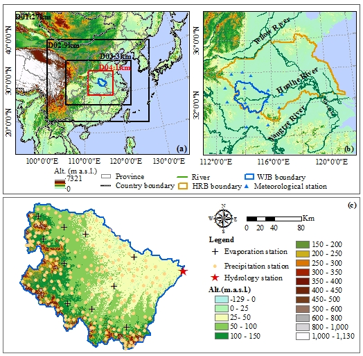
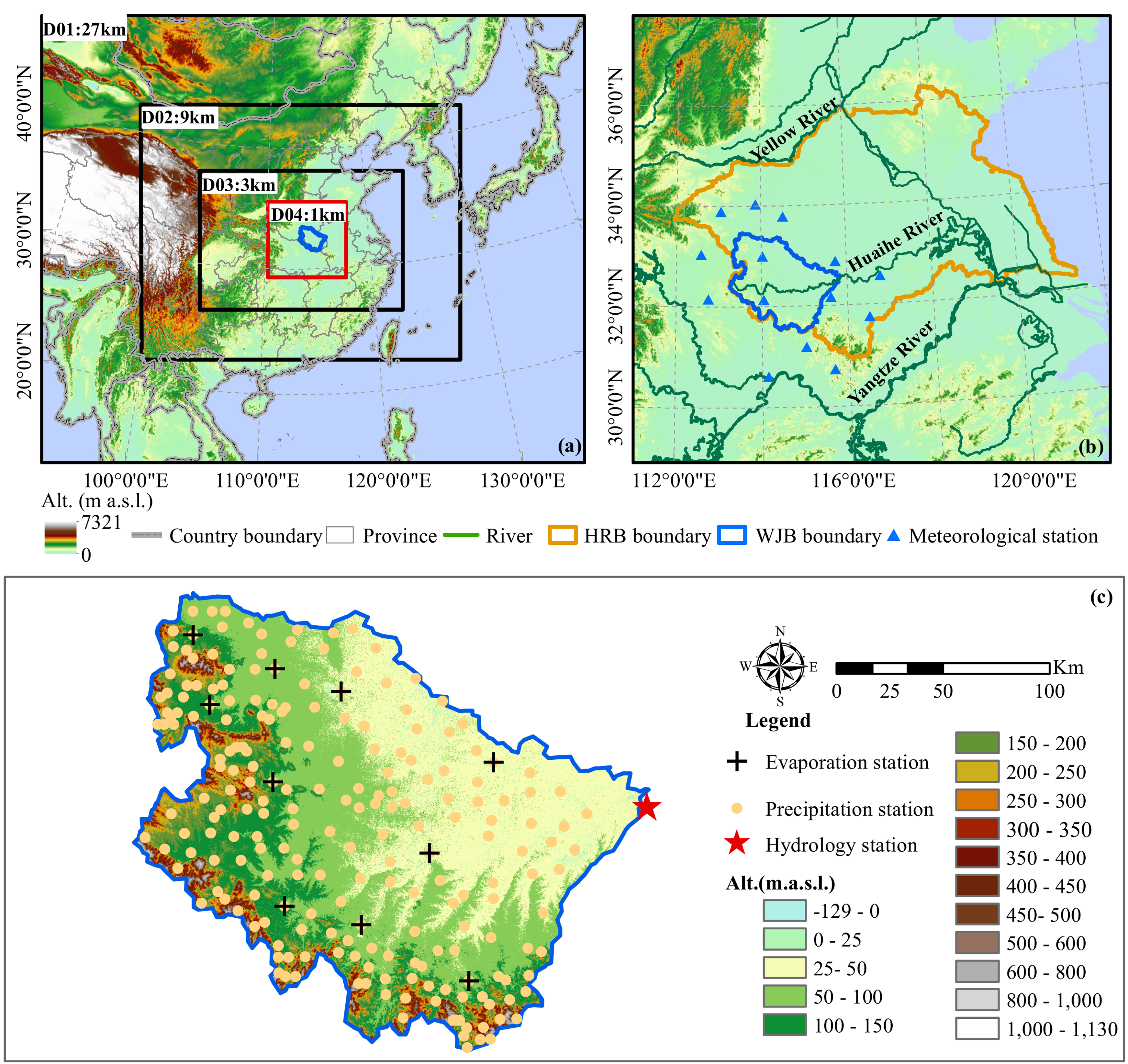
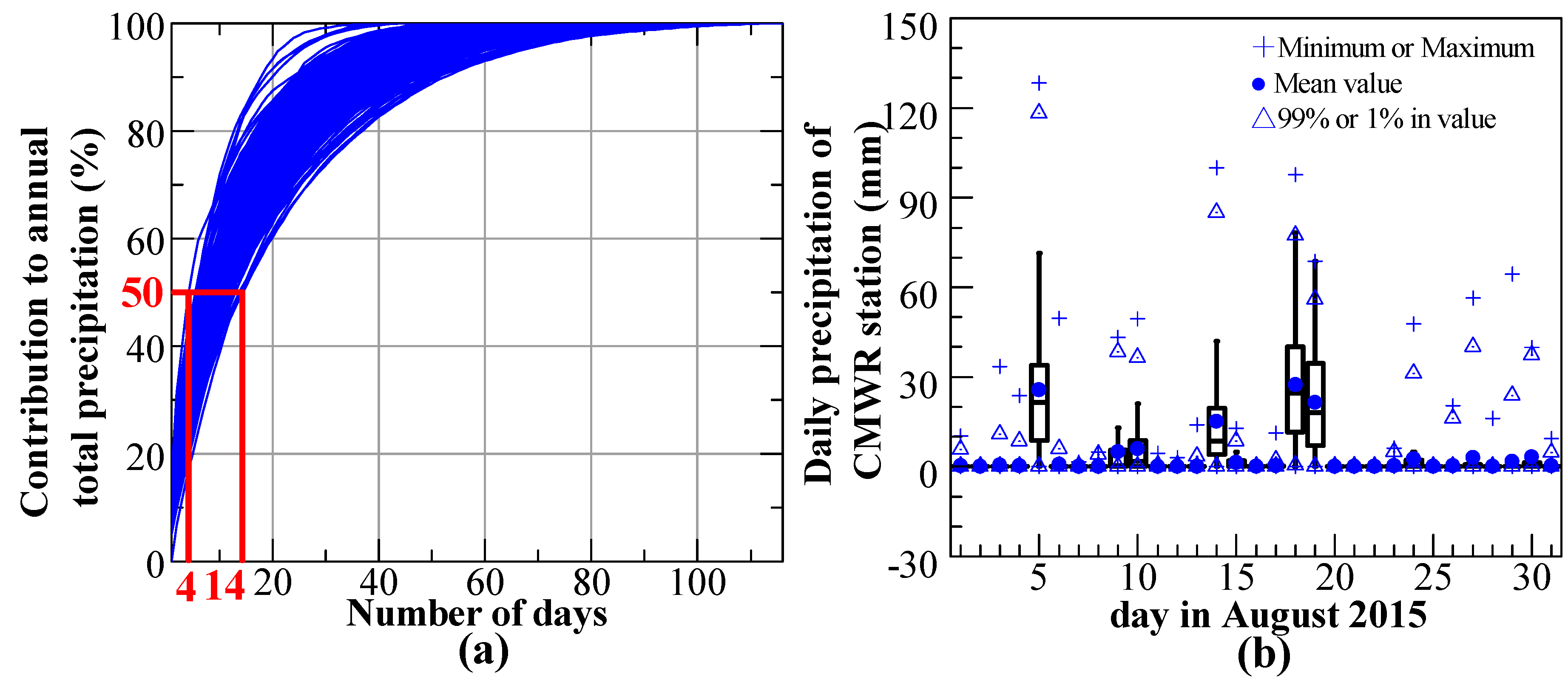
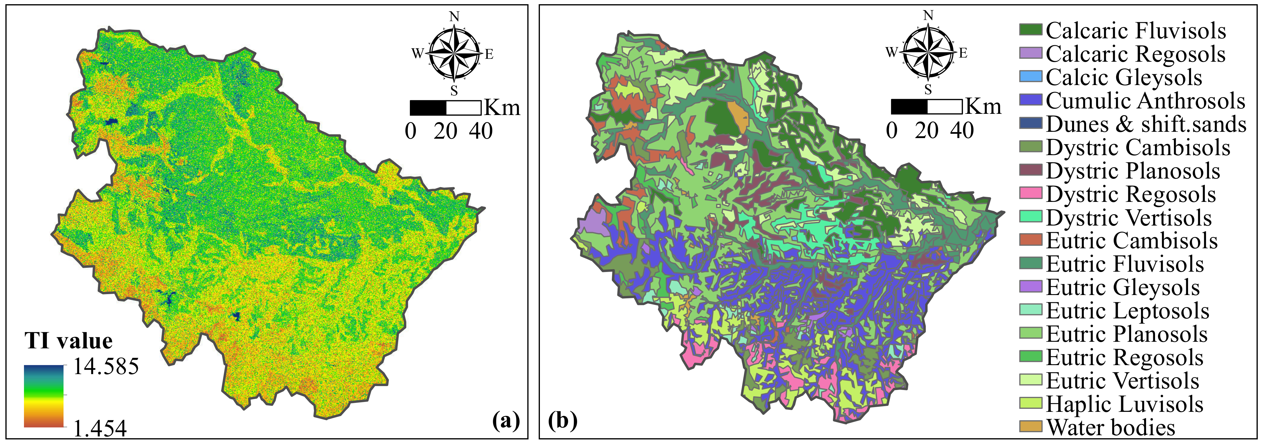
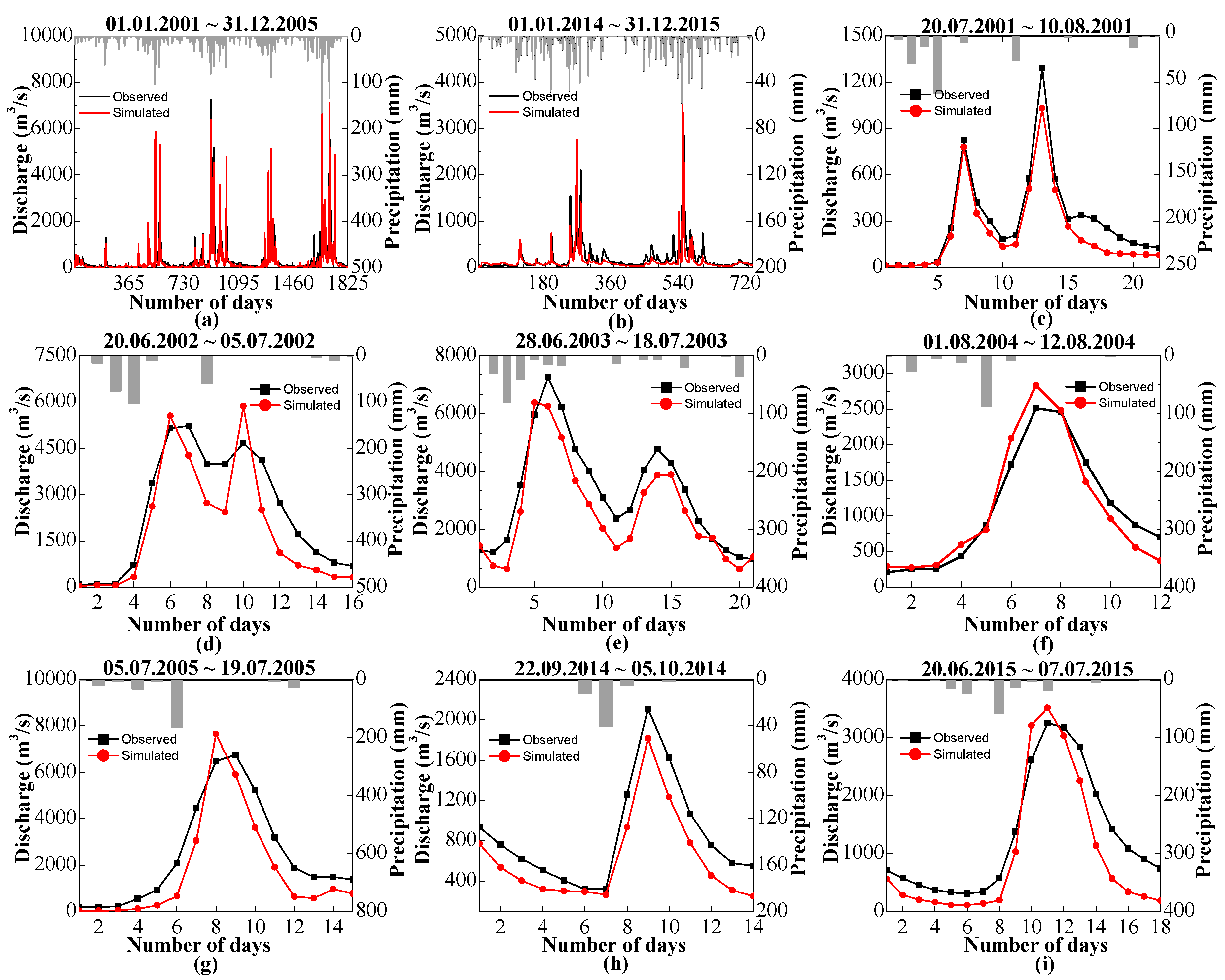
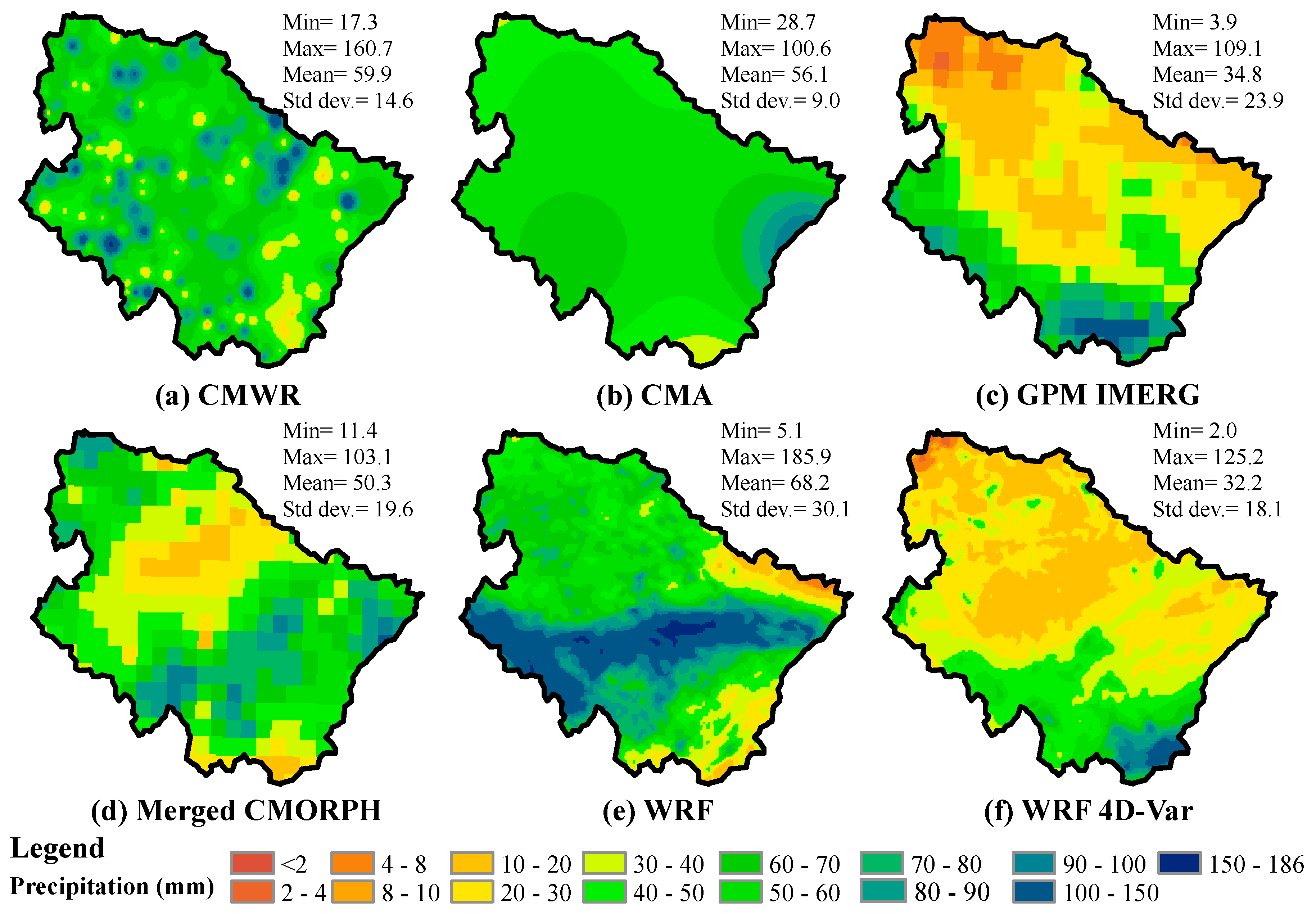
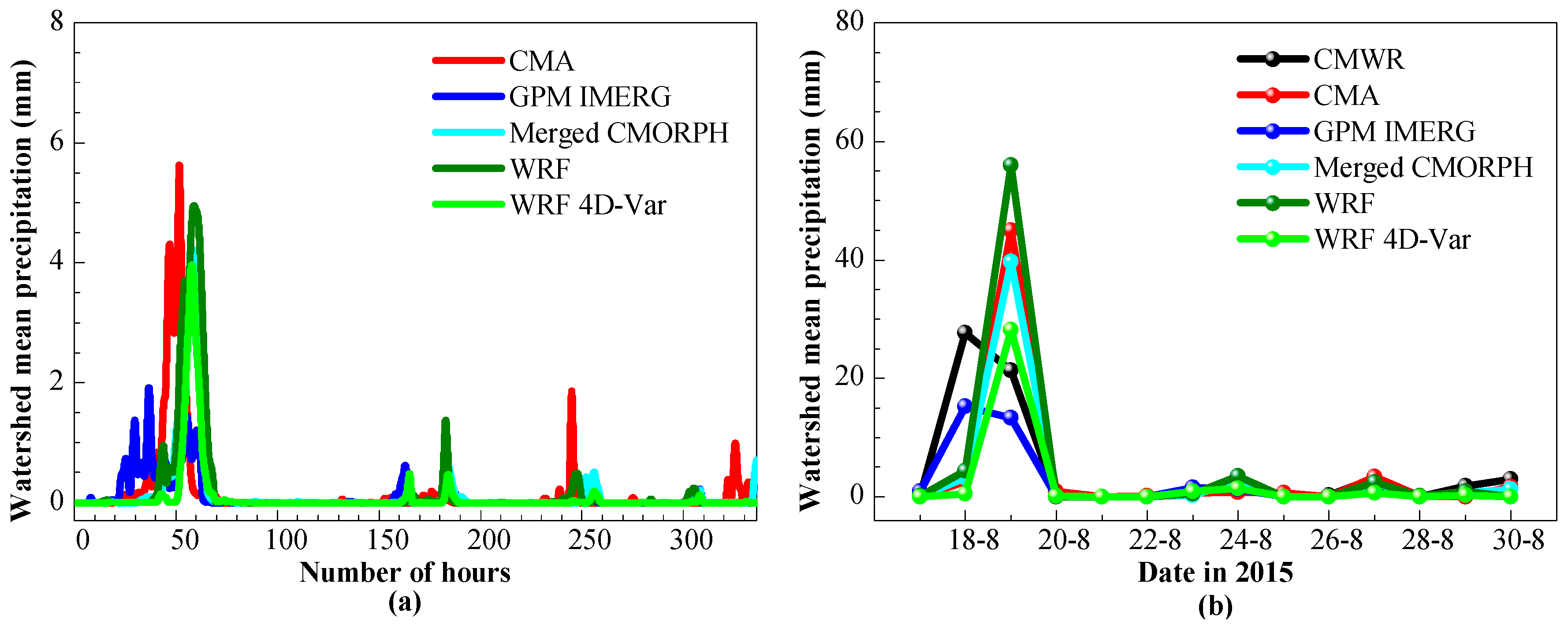
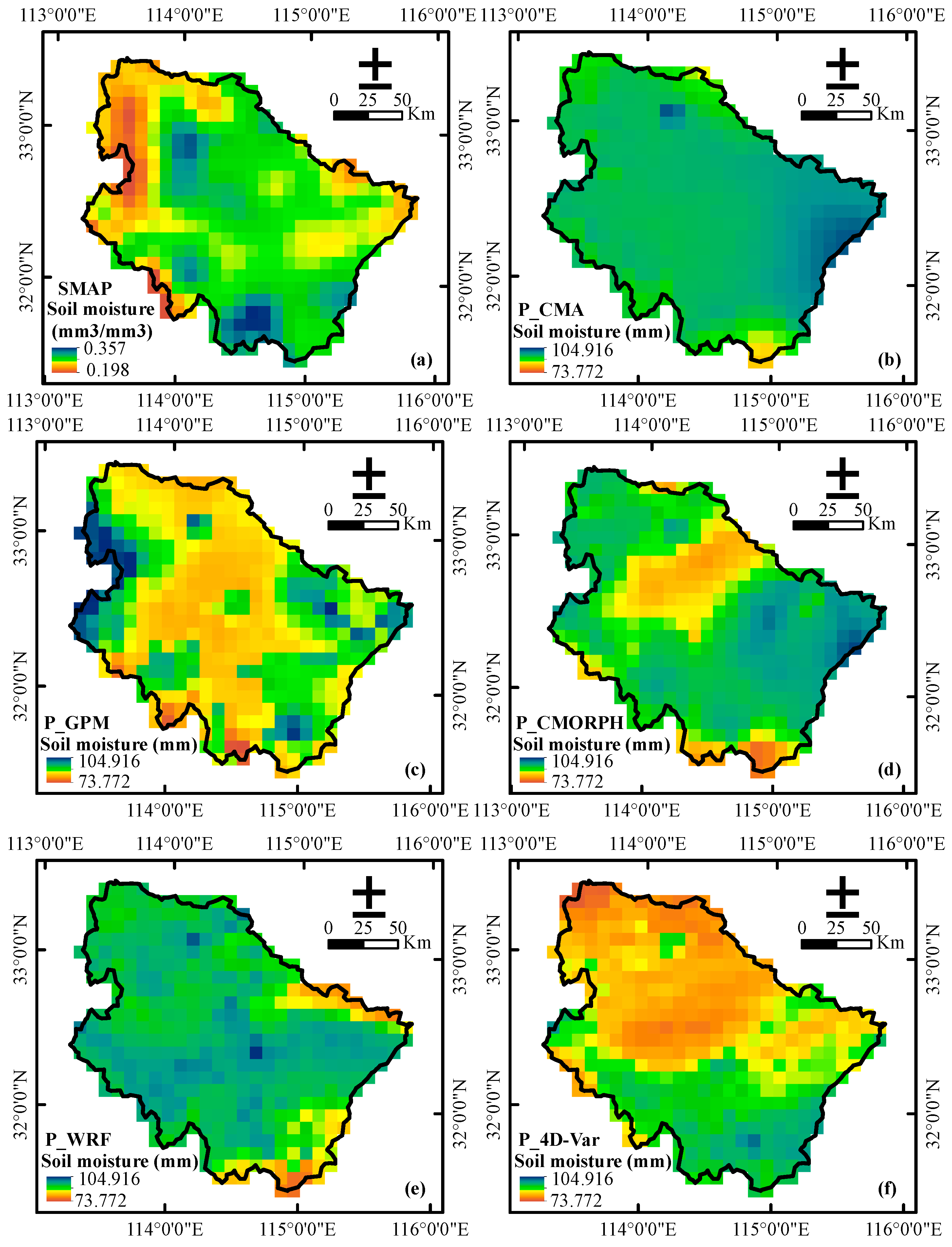
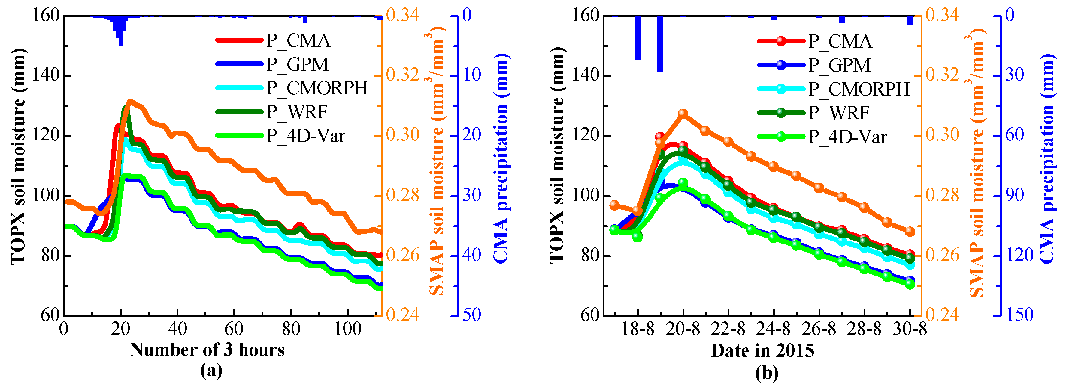
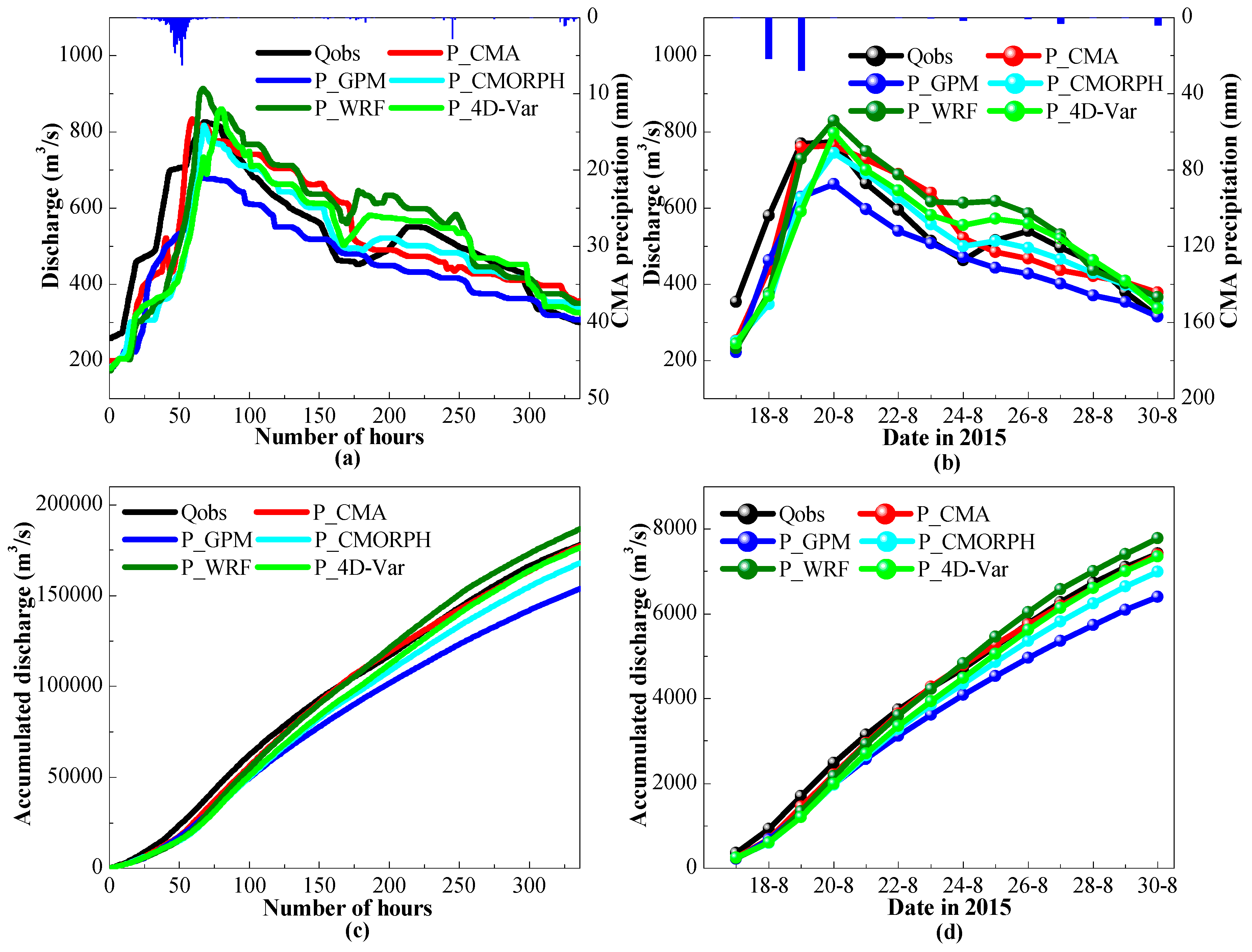
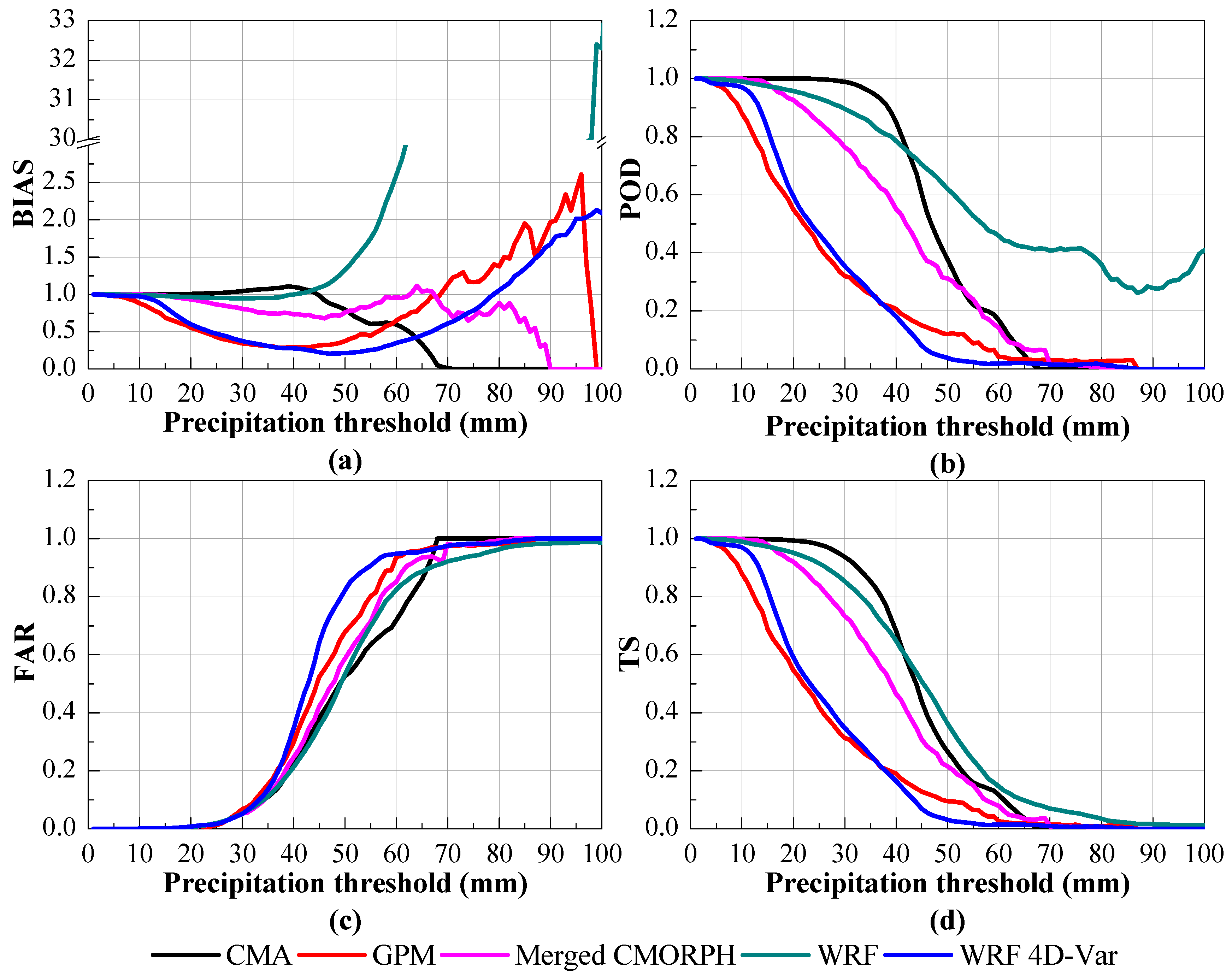
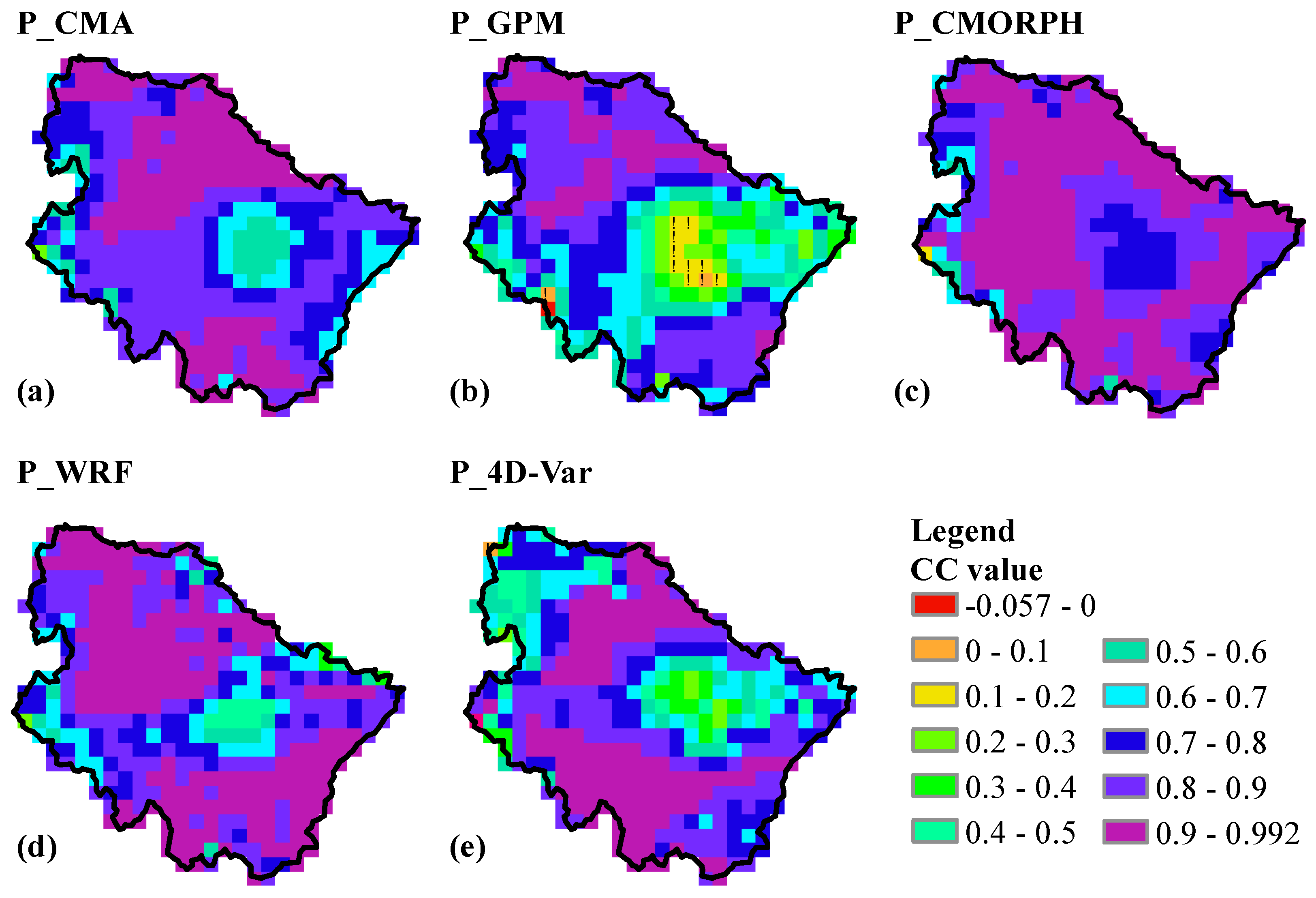
Table 1.
The main configuration of the WRF model.
| Map and Grids | |
|---|---|
| Map projection | Lambert conformal |
| Centre point of domain | 35.8°N, 114°E |
| Number of vertical layers | 27 |
| Horizontal grid spacing | 27 km, 9 km, 3 km, 1 km |
| Grids | 180 × 155, 322 × 271, 604 × 433, 700 × 700 |
| Static geographical fields | Standard dataset at 30″ resolution from the United States Geological Survey (USGS) |
| Time step | 150 s, 50 s, 17 s, 6 s |
| Physical Parameterization Schemes | |
| Cloud microphysics | WRF double-moment 6 scheme [93] |
| Long-wave radiation | Rapid radiative transfer model (RRTM) [94] |
| Short-wave radiation | Dudhia scheme [95] |
| Land-surface model | Noah land-surface model (LSM) [96] |
| Planetary boundary layer | Yonsei University scheme [97] |
| Cumulus parameterization | New Grell-Devenyi 3 scheme [98] (only in D01) |
Table 2.
Statistical results of the simulated daily discharges in the WJB watershed during the calibrations and validations of the hydrological model TOPX *.
Table 2.
Statistical results of the simulated daily discharges in the WJB watershed during the calibrations and validations of the hydrological model TOPX *.
| Simulation Time | NS | CC | RE | ||
|---|---|---|---|---|---|
| Long-term | Calibration | 1 January 2001~31 December 2005 | 0.787 | 0.898 | −0.292 |
| Validation | 1 January 2014~31 December 2015 | 0.700 | 0.857 | −0.248 | |
| Short-term | Calibration | 20 July 2001~10 August 2001 | 0.894 | 0.982 | −0.241 |
| 20 June 2002~05 July 2002 | 0.747 | 0.921 | −0.236 | ||
| 28 June 2003~18 July 2003 | 0.815 | 0.967 | −0.194 | ||
| 01 August 2004~12 August 2004 | 0.919 | 0.968 | −0.012 | ||
| 05 July 2005~19 July 2005 | 0.806 | 0.954 | −0.281 | ||
| Validation | 22 September 2014~05 October 2014 | 0.755 | 0.985 | −0.266 | |
| 20 June 2015~07 July 2015 | 0.772 | 0.953 | −0.251 | ||
* The indices of NS, CC and RE denote Nash-Sutcliffe coefficient, Pearson’s correlation coefficient and relative error, respectively.
Table 3.
Main parameters in the hydrological model TOPX.
| Parameter | Value |
|---|---|
| Decay factor (f, m−1) | 160 |
| Evapotranspiration coefficient (E) | 0.95 |
| Initial soil moisture content (W, mm) | 90 |
| Impact factor of vegetation root (C) | 0.12 |
| Maximum subsurface runoff (Rsb,max, mm) | 80 |
Table 4.
Experimental design for the rainfall-runoff simulations with different precipitation datasets.
Table 4.
Experimental design for the rainfall-runoff simulations with different precipitation datasets.
| No. | Experiment Label | Precipitation Category | Precipitation Data | Resolution of Precipitation Data |
|---|---|---|---|---|
| 1 | P_CMA | In situ observation | CMA data | Point scale, hourly |
| 2 | P_GPM | Remote sensing estimation | GPM IMERG | 0.1°, 30-min |
| 3 | P_CMORPH | Merged CMORPH | 0.1°, hourly | |
| 4 | P_WRF | NWP simulation | WRF output | 1 km, 6-s |
| 5 | P_4D-Var | WRF 4D-Var output | 1 km, 6-s |
Table 5.
Statistical metrics applied in the evaluations *.
| Statistical Metric | Equation | Perfect Value |
|---|---|---|
| Mean error (ME, mm) | 0 | |
| Relative error (RE) | 0 | |
| Root mean square error (RMSE, mm) | 0 | |
| Correlation coefficient (CC) | 1 | |
| Bias score (BIAS) | 1 | |
| False alarm ratio (FAR) | 0 | |
| Probability of detection (POD) | 1 | |
| Threat score (TS) | 1 | |
| Nash-Sutcliffe coefficient (NS) | 1 |
* PP,i and PO,i denote the simulated and observed values, respectively, of the i grid, and and are their respective means. A represents the precipitation predicted by the WRF and observed by the reference data; B represents the precipitation predicted by the WRF but not observed by the reference data; C represents the precipitation not predicted by the WRF but observed by the reference data; D represents the precipitation not predicted by WRF and not observed by the reference data. Qobs,i and Qsim,i are the observed and simulated values at time i; is the average value of the observations during the simulation period.
Table 6.
Error scores of mean error (ME), relative error (RE), root mean square error (RMSE) and Pearson’s correlation coefficient (CC) for the point-scale precipitation evaluations between the daily CMWR data and the daily grid data with 1-km resolution from different precipitation data.
Table 6.
Error scores of mean error (ME), relative error (RE), root mean square error (RMSE) and Pearson’s correlation coefficient (CC) for the point-scale precipitation evaluations between the daily CMWR data and the daily grid data with 1-km resolution from different precipitation data.
| Error Score | Precipitation Data | ||||
|---|---|---|---|---|---|
| CMA | GPM IMERG | Merged CMORPH | WRF Output | WRF 4D-Var Output | |
| ME | −0.424 | −1.489 | −0.805 | 0.159 | −1.868 |
| RE | −0.099 | −0.347 | −0.188 | 0.037 | −0.436 |
| RMSE | 11.719 | 10.112 | 11.577 | 13.411 | 11.946 |
| CC | 0.459 | 0.493 | 0.433 | 0.343 | 0.444 |
Table 7.
Statistics of Pearson’s correlation coefficient between the SMAP soil moisture and the soil moisture simulated by the rainfall-runoff experiments at 3-h and daily time scales.
Table 7.
Statistics of Pearson’s correlation coefficient between the SMAP soil moisture and the soil moisture simulated by the rainfall-runoff experiments at 3-h and daily time scales.
| No. | Experiment | Minimum 3 h/Daily | Maximum 3 h/Daily | Mean Value 3 h/Daily | Standard Deviation 3 h/Daily |
|---|---|---|---|---|---|
| 1 | P_CMA | 0.256/0.504 | 0.963/0.986 | 0.825/0.858 | 0.111/0.114 |
| 2 | P_GPM | −0.020/−0.096 | 0.967/0.986 | 0.695/0.705 | 0.208/0.235 |
| 3 | P_CMORPH | 0.197/0.477 | 0.992/0.996 | 0.885/0.891 | 0.091/0.093 |
| 4 | P_WRF | 0.259/0.186 | 0.986/0.992 | 0.841/0.852 | 0.132/0.136 |
| 5 | P_4D-Var | −0.057/0.067 | 0.983/0.993 | 0.774/0.780 | 0.183/0.194 |
Table 8.
Evaluation results of the hourly and daily outlet discharges simulated by the different rainfall-runoff experiments *.
Table 8.
Evaluation results of the hourly and daily outlet discharges simulated by the different rainfall-runoff experiments *.
| No. | Experiment | Hourly | Daily | ||||
|---|---|---|---|---|---|---|---|
| NS | CC | RE | NS | CC | RE | ||
| 1 | P_CMA | 0.658 | 0.855 | −0.003 | 0.694 | 0.876 | −0.003 |
| 2 | P_GPM | 0.576 | 0.919 | −0.137 | 0.582 | 0.935 | −0.137 |
| 3 | P_CMORPH | 0.596 | 0.823 | −0.057 | 0.621 | 0.837 | −0.057 |
| 4 | P_WRF | 0.464 | 0.816 | 0.048 | 0.499 | 0.832 | 0.048 |
| 5 | P_4D-Var | 0.547 | 0.787 | −0.010 | 0.560 | 0.796 | −0.010 |
* The indices NS, CC and RE denote Nash-Sutcliffe coefficient, Pearson’s correlation coefficient and relative error, respectively.
© 2018 by the authors. Licensee MDPI, Basel, Switzerland. This article is an open access article distributed under the terms and conditions of the Creative Commons Attribution (CC BY) license (http://creativecommons.org/licenses/by/4.0/).
Share and Cite
MDPI and ACS Style
Yi, L.; Zhang, W.; Li, X. Assessing Hydrological Modelling Driven by Different Precipitation Datasets via the SMAP Soil Moisture Product and Gauged Streamflow Data. Remote Sens. 2018, 10, 1872. https://doi.org/10.3390/rs10121872
AMA Style
Yi L, Zhang W, Li X. Assessing Hydrological Modelling Driven by Different Precipitation Datasets via the SMAP Soil Moisture Product and Gauged Streamflow Data. Remote Sensing. 2018; 10(12):1872. https://doi.org/10.3390/rs10121872
Chicago/Turabian StyleYi, Lu, Wanchang Zhang, and Xiangyang Li. 2018. "Assessing Hydrological Modelling Driven by Different Precipitation Datasets via the SMAP Soil Moisture Product and Gauged Streamflow Data" Remote Sensing 10, no. 12: 1872. https://doi.org/10.3390/rs10121872
Note that from the first issue of 2016, this journal uses article numbers instead of page numbers. See further details here.