Classification of Landslide Activity on a Regional Scale Using Persistent Scatterer Interferometry at the Moselle Valley (Germany)

Abstract

Landslides are a major natural hazard which can cause significant damage, economic loss, and loss of life. Between the years of 2004 and 2016, 55,997 fatalities caused by landslides were reported worldwide. Up-to-date, reliable, and comprehensive landslide inventories are mandatory for optimized disaster risk reduction (DRR). Various stakeholders recognize the potential of Earth observation techniques for an optimized DRR, and one example of this is the Sendai Framework for DRR, 2015–2030. Some of the major benefits of spaceborne interferometric Synthetic Aperture Radar (SAR) techniques, compared to terrestrial techniques, are the large spatial coverage, high temporal resolution, and cost effectiveness. Nevertheless, SAR data availability is a precondition for its operational use. From this perspective, Copernicus Sentinel-1 is a game changer, ensuring SAR data availability for almost the entire world, at least until 2030. This paper focuses on a Sentinel-1-based Persistent Scatterer Interferometry (PSI) post-processing workflow to classify landslide activity on a regional scale, to update existing landslide inventories a priori. Before classification, a Line-of-Sight (LOS) velocity conversion to slope velocity and a cluster analysis was performed. Afterwards, the classification was achieved by applying a fixed velocity threshold. The results are verified through the Global Positioning System (GPS) survey and a landslide hazard indication map.

1. Introduction

On all continents, landslides represent a major natural hazard which can cause significant damage, economic loss, and loss of life. Landslides can be defined as a downslope mass movement of rock, debris, or soil [1], and can be categorized with respect to the type of material (bedrock, debris, soil), the type of movement (fall, topple, slide, flow, complex), and the velocity [2].

Compared to other natural hazards (e.g., earthquakes, storms, or flooding), the impact of landslides is often underestimated because the affected areas are mostly on a local scale. Between 2004 and 2016, 55,997 fatalities caused by landslides were reported worldwide [3]. In Europe, it has been reported that landslides caused 312 fatalities and an economic loss of approximately 48 billion € in the timespan of 1998–2009 [4]. Landslide hazards are expected to increase in the future through population growth, new settlements in landslide-prone areas, and climate change [5].

Up-to-date, reliable, and comprehensive landslide inventories are mandatory for optimized disaster risk reduction (DRR) regarding landslides. Landslide risk can be defined as a measure of the expected probability of a damaging event for a specific area. It is based on the product of three factors: hazard, vulnerability, and exposure of elements at risk [6]. Landslide hazards can be defined as specific areas’ susceptibility to a potentially damaging landslide. For hazard assessments, landslide inventories are an important source of data. Conventional methods for the production of landslide inventories include things like the visual interpretation of stereoscopic aerial imagery, Light Detection and Ranging (LiDAR)-based digital surface models, and field surveys. A review of methods used for the production of landslide inventories is given by [7]. In general, landslide inventories lack information regarding the landslides’ state of activity, and are thus not up-to-date.

A new methodology for the updating of landslide inventories was recently proposed by the scientific community (e.g., [8,9,10]). These studies showed the potential of advanced Differential Interferometric SAR (DInSAR) methods (e.g., Persistent Scatterer Interferometry, [11]; Small Baseline Subset, [12]; SqueeSAR, [13]) for updating landslide inventory maps for large areas (up to 2100 km²). The major benefit of these methods is the provision of landslide movement information for large areas, with high precision and high temporal resolution. A standardization of procedures to classify the landslide state of activity, named the “PSI-based matrix approach”, was proposed by [14]. It focuses on the post-processing and comparison of PSI datasets covering successive time spans. The post-processing includes a conversion of the PSI LOS vector into the slope direction and the application of thresholds regarding the PSI-derived mean velocity and the minimum number of measurement points (persistent scatterer, PS) per landslide.

In this study, the “PSI-based matrix approach” is modified using a cluster analysis, instead of having a minimum number of PS per landslide as a precondition for the classification of the landslide’s state of activity. Our hypothesis was that the classification of the landslide’s state of activity would be more robust if a cluster of PSs with similar velocities is used, because the criterion for assigning a “representative velocity” to a landslide is not based on the number of PSs alone, but on a group of PSs with similar velocities. The clustering of PSs with similar velocities has been proposed by [15,16]. However, the clustering algorithm used in this work (local Moran’s Index) has not been proposed for landslide applications.

The second aim of this study was to demonstrate the capability of the German Ground Motion Service (BBD) for expanding landslide inventories with a classification of the landslide’s state of activity. The BBD PSI dataset was based on the recently-started Copernicus Sentinel-1 SAR mission. The Sentinel-1 mission is of particular interest because it ensures SAR data availability for almost the entire world, until at least 2030 (follow-on missions are in preparation). Long-term SAR data availability, and operationally available, advanced DInSAR products is a key precondition for the update of landslide inventories. The EC-FP7 project SAFER has proposed three services regarding landslide mapping and monitoring [9]:

• Landslide Inventory Mapping (LIM) for large areas covering a few thousand square kilometers;
• Landslide Monitoring (LM) for single large landslides affecting built-up areas with a high risk level;
• Rapid Landslide Mapping (RLM) carried out after an emergency for rapid mapping of pre-existing landslides with potential reactivations and new landslides.

Using this service definition, this study focuses on the procedure of performing a LIM.

2. Study Area

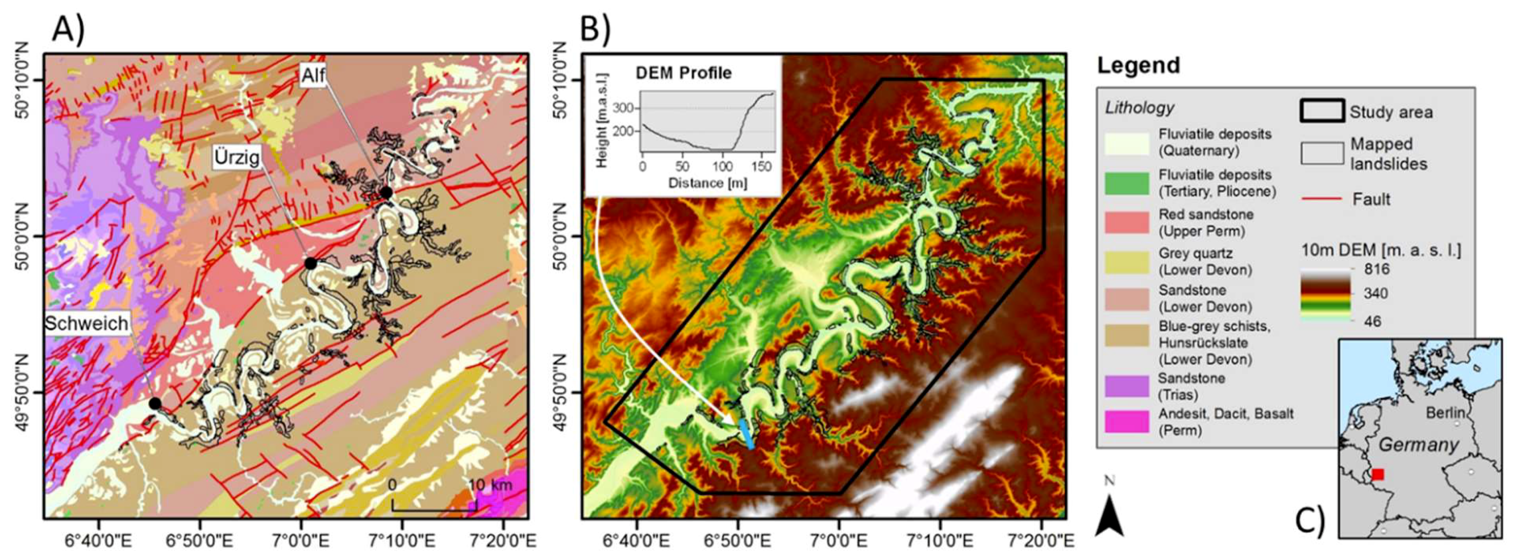
The study area had a size of approximately 1500 km² and is located at the Moselle Valley, Germany. The Moselle Valley has different elements at risk, such as settlements, tourist attractions, federal roads, and a highway under construction. The river Moselle flows from the southwest to the northeast, and divides the low mountain ranges of the Hunsrück in the south from the Eifel in the north. The river enters the study area at a height of 123 m.a.s.l. and leaves it at a height of 78 m.a.s.l., with a height difference of 45 m along with a distance of 145 km. The adjacent plateau and mountain ridges reach heights of more than 400 m.a.s.l. (Figure 1B). The geomorphology is characterized by narrow, V-shaped valleys with a pronounced meandering of the river, causing distinct slip-off banks and undercut slopes. While the slip-off banks are relatively flat, some of the undercut slopes are very steep (transect in Figure 1B) and reach inclinations of more than 40°. The majority of the slopes have inclinations below 30°. The slopes with a southwest-, southeast- and south exposition are often used for winegrowing. Most of the north-facing slopes and the upper slope areas are covered with forests. On steep undercut slopes, bare rocks emerge, and settlements are often at the foot of the slopes.

The geology of the study area is almost completely composed of Lower-Devonian Hunsrückslate (Unterems). The Hunsrückslate is a monotone, anchimethamorph sequence of approximately 3000 m-thick clay and siltstones, with sporadic occurrence of thin quartzitic sandstones and slates [17]. At the southwestern border of the study area, near the village Schweich, a sequence of grayblue argillaceous schists with gravelsized concretions is present. Near the village Ürzig, light-red siliciclastics and tuffs are present. Near the village Alf, the Mosel Valley leaves the Hunsrückslate and enters an area composed of clay and sandstones, belonging to the Oberems/Devonian Laubach- and Hohenrhein sequence (Figure 1). All rock units were folded and foliated during the Variscian orogeny. Tectonically, the area belongs to the southeast-vergent Moselle depression. Since the Tertiary, the Rhenish Shield has been affected by largescale uplift, which is still ongoing. Multiple changes in the tectonic stress caused deep fragmentation of the rocks.

The fast incise of the Moselle Valley induced steep slopes with high relief energy. These young slopes are morphologically immature, and not yet in equilibrium. Evidence of the low slope stability is given by things such as landslides, rockfalls, tilting of houses, and cracks in roads.

Landslides are defined as a downslope mass movement of rock, debris, or soil [1]. They can be categorized with respect to the type of material (bedrock, debris, soil), the type of movement (fall, topple, slide, flow, complex), and the velocity [2].

The majority of landslides in the study area are large, deep-seated slides, which are often located at the undercut slopes. The landslides are located between 80 and 427 m.a.s.l. Some of the landslides are in built-up areas and crossed by roads. The geomorphology often consists of convex, upper slope areas, and concave, lower slope areas. The DEM profile in Figure 1B represents the characteristic geomorphology of slopes at the river Moselle. In general, the landslides in the study area are related to the occurrence of the Hunsrückslate. Most of the displacements in the upper areas are in vertical direction, while in the convex lower parts of the landslides, horizontal displacements dominate. Besides the deep-seated slides, creeping soils/debris are present on relatively steep slopes where the soils/debris are characterized by low permeability. The highest measured debris slide velocity in the study area reaches up to 16 cm per year [20].

3. Methodology and Data

The methodology consists of four steps: (i) PSI-processing; (ii) transformation from v_LOS into v_SLOPE; (iii) cluster analysis; and (iv) classification of the landslide’s state of activity. The classification results are verified with a landslide hazard indication map.

3.1. PSI-Processing

The PSI dataset used in this work was processed by the German Aerospace Center (DLR). DLR was contracted in the framework of the German Ground Motion Service (BBD) for PSI-processing. PSI processing starts with the detection of PS candidates by thresholding the Signal-to-Clutter ratio (SCR) in the coregistered SAR data stack [21]. Afterwards, the PS candidates are geocoded, and a grid with a cell size of about 1 km is created and superimposed onto the PS candidates. Based on the grid, the PS candidates with the highest phase stability are extracted from each grid cell. The extracted PSs build the basis of the reference network. For all arcs of the reference network [22], the height update, mean velocity, and the atmospheric phase screen (APS) are estimated. Now, a robust L1-norm network inversion is performed for outlier removal [23,24], and a PS reference point is selected. Afterwards, the residual height, mean velocity, and the displacement time series are estimated for each PS in the reference network, by performing an L2-norm network inversion. After the removal of the estimated APS, all the PS candidates which are not included in the reference network are connected to the PSs from the reference network. Finally, for all PSs, the residual height, mean velocity, and the displacement time series are estimated relative to the PS reference point.

Typically, PS are related to man-made structures (e.g., houses, bridges, railways, roads) or natural objects (rock outcrops, boulders).

The Sentinel-1 SAR dataset used in this study covers the timespan from 15 October 2014 until 1 July 2017, and consists of 66 acquisitions, with an incidence angle of 40° in the middle of the study area and a satellite heading of 195° (descending orbit). An improved version of the 3 arc-second SRTM C-band DEM [25] was used to calculate and remove the topographic phase from the interferograms.

3.2. Conversion from v_LOS into v_SLOPE

PSI is a one-dimensional measurement technique; thus, the mean velocity and displacement time-series of a PS is measured in the satellites’ Line-of-Sight (LOS). Positive LOS values represent a displacement towards the satellite, while respective negative LOS values represent a displacement away from the satellite. In order to use the LOS velocities with respect to the detection of displacements caused by landslides, a conversion of the LOS velocity vector (v_LOS) into slope direction (v_SLOPE) is performed (e.g., [14,26,27]). The conversion is based on the assumption that the displacement is purely parallel to the maximum slope direction. The conversion is performed by using the following equations [27]:

$$v_{SLOPE}=\frac{v_{LOS}}{C}$$

(1)

The C coefficient represents the sensitivity of the LOS vector to measure a displacement in slope direction. It is calculated by:

$$C=N·\left(\cos \left(S\right)·\sin \left(A-90\right)\right)+E·\left(-1·(\cos \left(S\right)·\cos \left(A-90\right)\right)+H·\left(\sin \left(S\right)\right)$$

(2)

where A is the terrain aspect with respect to the North, and S is the slope angle. N, E, and H are the directional cosines of the LOS vector, and are calculated by using:

$$N=\cos \left(90-\mathsf{\theta }\right)·\cos \left(180-\mathsf{\alpha }\right)$$

(3)

$$E=\cos \left(90-\mathsf{\theta }\right)·\cos \left(270-\mathsf{\alpha }\right)$$

(4)

$$H=\cos \left(\mathsf{\theta }\right)$$

(5)

where θ is the incidence angle and α is the satellite ground track angle (approximately −15 degrees for ascending orbit and approximately −165 degrees for descending orbit) plus 90 degrees. A digital elevation model (DEM) with a spatial resolution of 10 × 10 meters is used to calculate the terrain aspect and inclination of the slopes in the study area. The DEM is based on a compilation of different data sources (LiDAR, stereoscopic aerial imagery, and digitized topographic maps) and a vertical and horizontal accuracy of 0.5–2 m is reported [19]. For areas with very low sensitivity, C values approach zero and the v_SLOPE tends to infinity; thus, in order to prevent an artificial exaggeration of the v_SLOPE, the C-value is fixed to −0.3 if −0.3 ≤ C < 0 and to +0.3 if 0 ≤ C ≤ +0.3. As a consequence, the v_SLOPE cannot be higher than 3.33 times v_LOS. The v_LOS scaling factor limit of 3.33 is based on [28], where a comparison of v_SLOPE values with differential GPS measurements has shown that this is an appropriate threshold.

3.3. Cluster Analysis

The result of the conversion is used as input for the cluster analysis. The cluster analysis uses v_SLOPE as an input variable for the detection of PS clusters. The cluster analysis is based on the null hypothesis that there is no association between v_SLOPE values in nearby PSs. The alternative hypothesis is that spatial clustering exists, meaning that nearby PSs have similar v_SLOPE values. The result of the cluster analysis is the local Moran’s I Index, the z-score, the p-value, and the code characterizing the cluster type. The local Moran’s Index ($I_i$) is calculated by using the following equations [29]:

$$I_i=\frac{x_i-\overline{X}}{S_i^2}{\displaystyle \sum }_{j=1,j\ne i}^n{w}_{i,j}\left(x_j-\overline{X}\right)$$

(6)

and:

$$S_i^2=\frac{{{\displaystyle \sum }}_{j=1,j\ne i}^n{\left(x_j-\overline{X}\right)}^2}{n-1}$$

(7)

where $x_i$ is the v_SLOPE value for the $i$’th PS, $\overline{X}$ is the mean of the v_SLOPE of all PSs, n is the total number of PSs, and $w_{i,j}$ is the spatial weight between the PSs $i$ and $j$. The spatial weight is based on an inversed square distance model to describe the spatial relationship. Thus, only close PSs have an influence on the local Moran’s I Index. As the precision of the estimated PSI velocity decreases over distance mainly due to a residual tropospheric phase and error propagation (e.g., [30,31]), an upper threshold of the neighborhood search radius of 200 m is set.

In order to assess the significance of the cluster analysis, a randomization procedure is performed. For this reason, the locations of the PSs are randomly reconfigured n times (in this case, n = 499). The distribution of local Moran’s I Index based on these permutations is then compared with the local Moran’s I Index computed from the original PS locations. By doing so, it is possible to assess the probability that the results of the cluster analysis come from a random distribution. By using 499 permutations, the smallest possible p-value is 0.002, meaning that the minimum of the calculated probability of being wrong (e.g., PSs are falsely classified as a cluster) is 0.2%. In this study, the upper threshold for the p-value is set at 5% to account for statistical significance of the detected PS clusters.

A high value of $I_i$ indicates that a PS has similar v_SLOPE values as the neighboring PSs. In general, these PS clusters can consist of either positive or negative v_SLOPE values. Positive v_SLOPE values represent an uphill movement, and have been discarded. Although a vertical uplift may occur at the feet of landslides, the velocity vector in a slope direction (v_SLOPE) should remain downhill, because a dominant uphill movement, of very slow landslides, is not plausible. The result of the cluster analysis is statistically significant PS clusters, indicating downhill movement. These PS clusters are the input for the classification of the landslides’ state of activity.

3.4. Classification of the Landslides’ State of Activity

The velocity of a landslide can be correlated with the damage it may cause [32]. The International Union of Geological Sciences Working Group on Landslides established a classification of landslide velocities in order to extend the Landslide Report within the World Landslide Inventory. This official classification of landslide velocities spans ten orders of magnitude. It consists of seven velocity classes, and ranges from 16 mm per year to 5 m per second [32]. The official classification is based on well-described landslides, where the peak velocity during an exceptional behavior phase and information regarding damages are available. A comparison between peak velocities and observed damages reports is that the peak velocity class, “extremely slow” (peak velocity ≤ 16 mm per year), corresponds to “No damage to structures built with precautions”, and the peak velocity class, “very slow” (peak velocity ≤ 1.6 m per year), corresponds to “Some permanent structures undamaged or, if they are cracked by the movement, they can be repaired” [32]. The relation between peak velocity and damage is not straightforward, because damage also depends on things like the internal distortion of the displaced mass, the margin of the displaced mass, and the type of landslide. Thus, the official velocity classes are schematic, because the peak velocity alone may not give a sufficient characterization of the landslide processes (e.g., at the margin of a landslide) [32]. However, it offers a practical method to include information on landslide velocity in a landslide report.

In contrast to the official landslide velocity classes, the PSI technique does not measure the maximum velocity during an exceptional behavior phase. PSI provides the mean velocity of several years in the direction of a Line of Sight. Consequently, the choice of a proper threshold is a key step, and needs to take the following aspects into account [14]: the type of the observed deformation process (e.g., geometry, expected velocity), technical characteristics of the PSI data (e.g., LOS geometry), and post-processing steps (e.g., reprojection of LOS velocity into slope velocity). Recent studies at a regional scale have used LOS velocity thresholds ranging from 1.5 to 10 mm per year to classify active landslides [8,33,34,35]. A literature review from [36] identified a threshold of 10 mm per year, where moderate damage is present at buildings and infrastructure. [8,37,38] used the 10 mm per year threshold to classify active landslides using advanced DInSAR data.

In this study, a threshold of 10 mm per year was used to classify active landslides. This choice was driven by the following reasons: The PSI-based velocity is a mean velocity over several years, while the official threshold of 16 mm per year discriminating “extremely slow” from “very slow landslides” (which correlates with damages) refers to peak velocities [1]. As observed by [34], peak velocity may significantly exceed the mean velocity. Thus, a mean velocity threshold should be lower than a peak velocity threshold. Furthermore, a threshold lower than 16 mm per year reduces the probability of discarding potentially active landslides, assuring that even slow landslides with certain damage potential are classified as active [38]. On the other hand, the threshold must not be lower than the precision of the PSI dataset [34], which needs to be controlled prior to the cluster analysis. The PSI dataset used in this study has an uncertainty of 2σ < 1.2 mm per year caused by clutter [39]. Another reason not to use a very low threshold, such as 2 mm per year, is the conversion from LOS to slope direction. The conversion will amplify any noise in the PSI data, especially in areas with low sensitivity, such as slopes with an exposition approximately towards the North or the South.

In order to classify the landslides’ state of activity based on landslides mapped a priori, the result of the PS cluster analysis was intersected with the landslide polygons. If the maximum v_SLOPE value of a PS, belonging to a PS cluster that intersects with a landslide polygon, is faster than 16 mm per year, the landslide is classified as “Active, very slow”. If the maximum v_SLOPE value of a PS, belonging to a PS cluster that intersects with a landslide polygon, is between 16 and 10 mm per year, the landslide is classified as “Active, extremely slow”. If the maximum v_SLOPE value of a PS in a landslide polygon is less than 10 mm per year, the landslide is classified as “Inactive”. If no PS cluster intersects with a landslide polygon, the polygon is classified as “Not classified”.

3.5. Ancillary Data

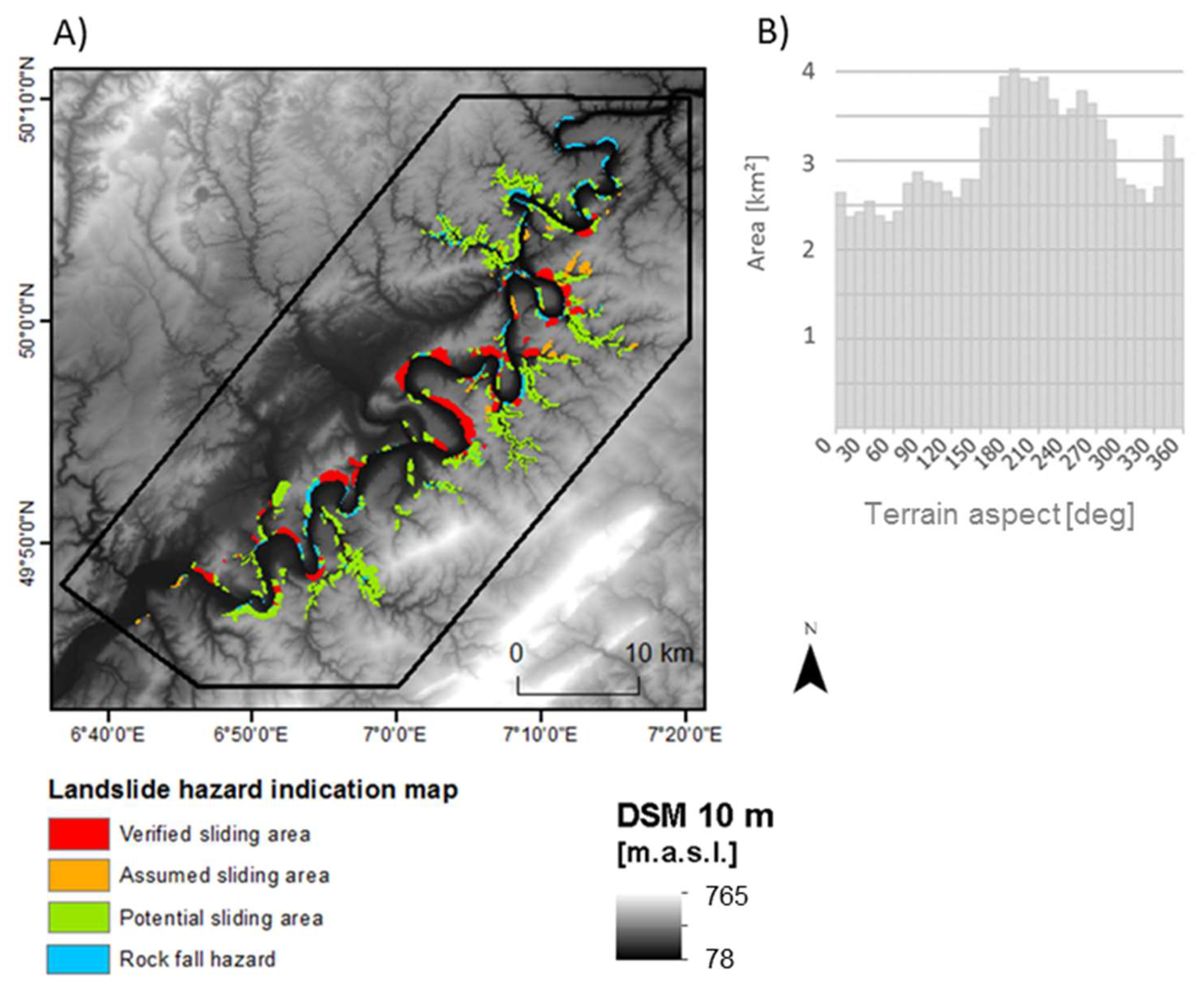
The a priori mapped landslide polygons used in the classification of the landslides’ state of activity is based on a landslide hazard indication map published by [40]. The purpose of this map is to give an areal indication of landslide hazards on a scale of 1:50,000. The map includes 383 sliding areas with an average size of 0.152 km² (Figure 2A). The landslides are located between 80 and 427 m.a.s.l., the maximum slope inclination is 67°, and the average slope inclination is 22°. The distribution of the slope exposition of the landslide areas is shown in Figure 2B. It shows that 20.6% more landslide areas are facing to the West (260–280°) than to the East (80–100°). Generally, SAR data from ascending acquisitions are suitable for slopes facing to the East, where the movement direction is likely to be toward the East. SAR data from descending acquisitions are suitable for slopes facing to the West, where the movement direction is likely to be towards the West [14]. Thus, the descending satellite orbit is better suited for this study area.

The landslide hazard indication map is based on archive documents of the state Geological Survey (Landesamt für Geologie und Bergbau Rheinland-Pfalz), stereoscopic aerial imagery, LiDAR data, and field surveys [41]. Visual image interpretation of the aerial imagery and geomorphological analysis of the LiDAR data were performed and verified by field surveys. The result categorized four landslide hazard indication classes: “verified sliding area”, “assumed sliding area”, “potential sliding area”, and “rockfall area”. A landslide is classified as “verified sliding area” if the sliding mass has pronounced differentiation of terrain humps, plain terrace surfaces, and head scarps. If such a landslide is located in a vineyard area, strong indications of active movements are often visible, such as roads with cracks, deformed walls, and tilted vine stocks. If the sliding mass has unclear geomorphological features, such as that the head scarp cannot be distinguished unambiguously, it is classified as “assumed sliding area”. Areas with a theoretical potential of landslides are classified as “potential sliding area”. The potential is derived by using datasets regarding the geological and geomorphological setting, and land use. It can be assumed that landslides occur in these areas only after large load changes or massive anthropogenic activities, such as terrain cuts. Areas with a significant rockfall hazard are classified as “rockfall areas”, generally located at slopes with a mean slope angle of more than 45°. The landslide hazard indication map includes the rockfall source areas and the deposition areas (Figure 2).

The landslide hazard indication map does not include an in-depth landslide analysis or a risk assessment. However, the class “verified sliding area” is a strong indicator of recent or ongoing soil-creeping processes. Thus, a plausibility assessment of the classification of the landslides’ state of activity is performed by using the category, “verified sliding area”.

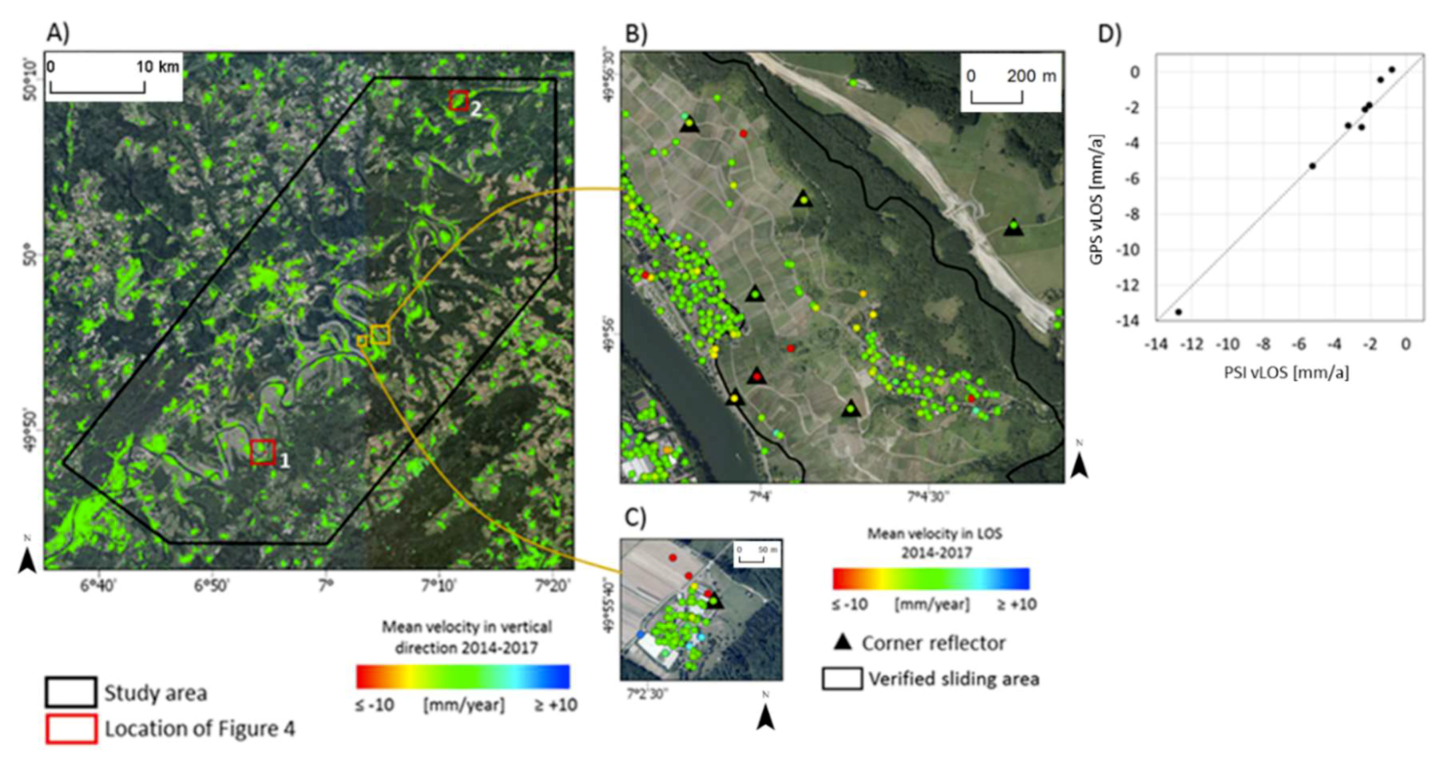
In order to verify the Sentinel-1 PSI data, eight PSs located at corner reflectors were compared with a series of nine differential GPS surveys. The corner reflectors were installed on 6 October 2010 and on 12 October 2011 to monitor an active landslide [42]. The corner reflectors were installed to increase the PS density in this area. The area was of particular interest because of a road construction in the vicinity of the landslide. The dimension of the trihedral corner reflectors were specified to fit the requirements of PSI analysis based on TerraSAR-X Stripmap data from a descending orbit with an incidence angle of 43°. The construction design consisted of concrete with integrated metal plates to resist harsh weather conditions, vandalism, and theft. Although the dimension and orientation of the corner reflectors were chosen to meet the requirements of TerraSAR-X (X-band) acquisitions, the corner reflectors were detected as PS in the Sentinel-1 (C-band) dataset. For Sentinel-1, the average LOS displacement 2σ-error at the corner reflectors sites was 0.9 mm, the corresponding effective phase noise was 0.2 radians (2σ), and the signal-to-clutter ratio was 10.5. Six corner reflectors were located in an area classified as a “verified sliding area” in the landslide hazard indication map. Two corner reflectors were located outside a “verified sliding area” (Figure 3C and the corner reflector in the East in Figure 3B). The differential GPS surveys were conducted by the State Office for Mobility [40] and took place on the following dates: 25 November 2014, 24 February 2015, 28 May 2015, 25 August 2015, 2 December 2015, 31 March 2016, 31 August 2016, 6 December 2016, and 22 March 2017. A linear regression was performed to estimate the mean velocity in the directions of X, Y, and Z. For the comparison with the Sentinel-1 LOS velocity, the 3D GPS velocity vectors were projected into the direction of SAR LOS. In order to quantify the horizontal geocoding precision caused by satellite timing error and the APS of the SAR master scene, the mean deviation between the eight PSs at the corner reflectors and the precise position of the corner reflectors were calculated.

4. Results

In the study area, a total of 95,373 PSs were detected, resulting in an average spatial sampling density of 63.6 PS per km². The majority of PSs were located in cities, villages, and transport infrastructure (roads, railways, bridges) (Figure 3A). Stonewalls, guardrails, and street signs were present at these small roads and paths, and often corresponded to PSs. The landslide areas were often used for vinery and crossed by small roads and paths (Figure 3B).

The verification results shows a mean difference between the PSI and GPS velocity of 0.49 mm per year (2σ = ± 0.37 mm per year). A scatterplot visualizes the high correlation between PSI and GPS velocity (Figure 3D). Note that the GPS-based mean velocity (2014–2017) is based on nine measurement dates, while the PSI-based mean velocity (2014–2017) is based on 66 measurement dates. Although a linear displacement rate is assumed in both datasets, the difference in temporal resolution can bias a comparison of PSI and GPS velocities, if a strong non-linear displacement is present. The horizontal position of the eight PSs at the corner reflector sites had a mean deviation of 7.2 m with respect to the precise corner-reflector position.

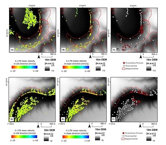
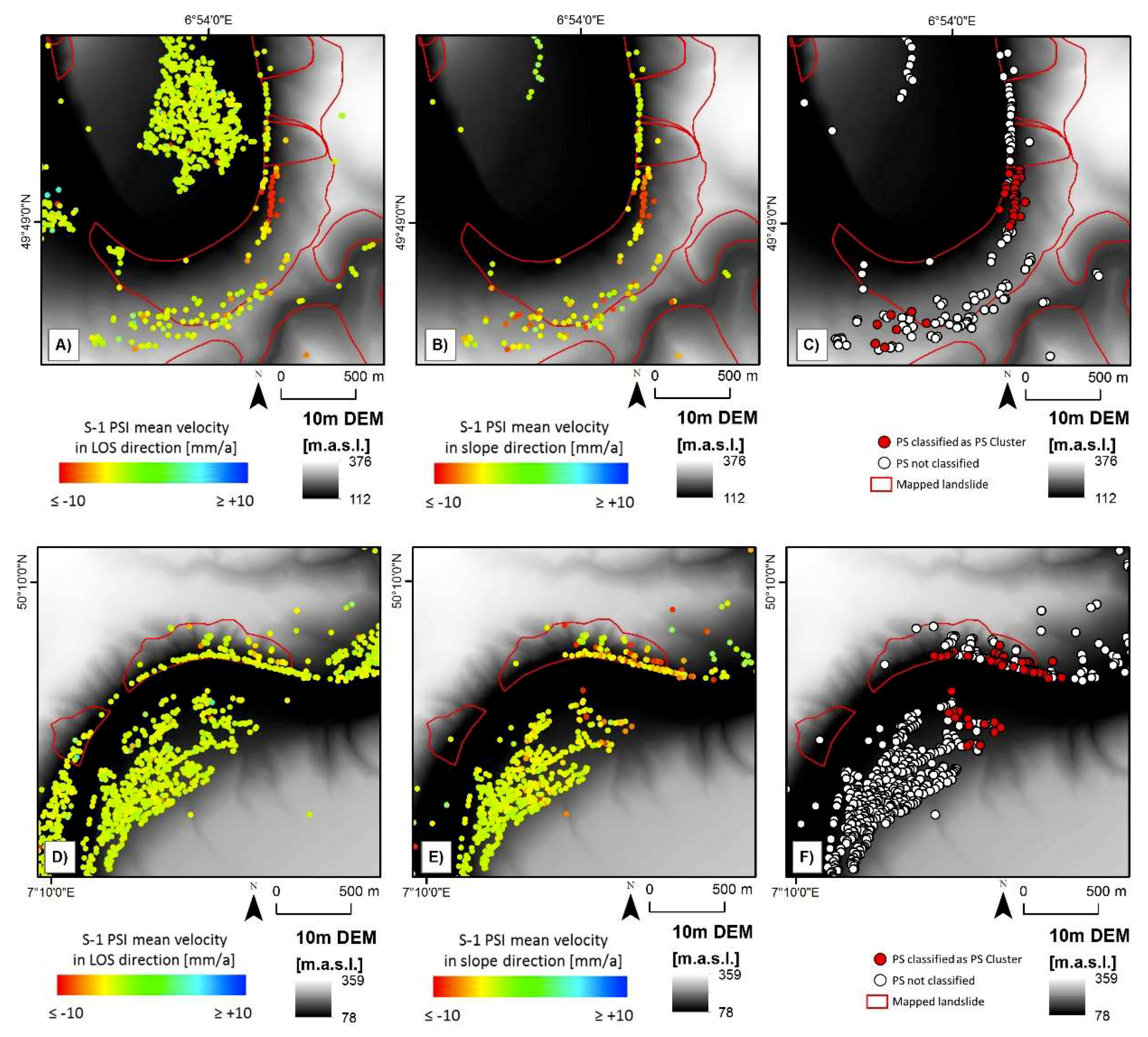
The results of the conversion of the PSI LOS mean velocity into the mean velocity in slope direction is shown in Figure 4B,E, where positive mean velocities (representing an uphill displacement), as well as PSs located in flat areas (slope inclination ≤ 4°) are discarded meaning that the number of PSs is reduced by 78.3%. The consequence of this reduction is a reduced completeness in classification, but the exclusion of implausible v_SLOPE values is expected to increase the classification correctness. The results of this reduction and the results of the conversion are exemplarily shown in Figure 4A,D (before reduction) and in Figure 4B,E (after reduction). The PSs with a v_LOS mean velocity of approximately −10 mm per year present in the center of Figure 4A are affected very little by the conversion (Figure 4B). The reason for this is the slope exposition, which is very similar to the satellite heading and also similar to the slope angle to the SAR incidence angle. Consequently, the sensitivity of the SAR imaging geometry to measure displacements in slope direction is between 90% and 95% in this area. The strong impact of the LOS conversion for South-facing slopes is visualized in Figure 4D,E. Due to the low sensitivity in these areas, the C-value reaches its upper value of 0.3. The results of the conversion are the input for the subsequent PS cluster analysis. The results of the PS cluster analysis are exemplarily shown in Figure 4C,F. The cluster of PSs characterizing a similar slope displacement, visible in the v_SLOPE map (Figure 4B,E), are successfully detected as a cluster (Figure 4C,F).

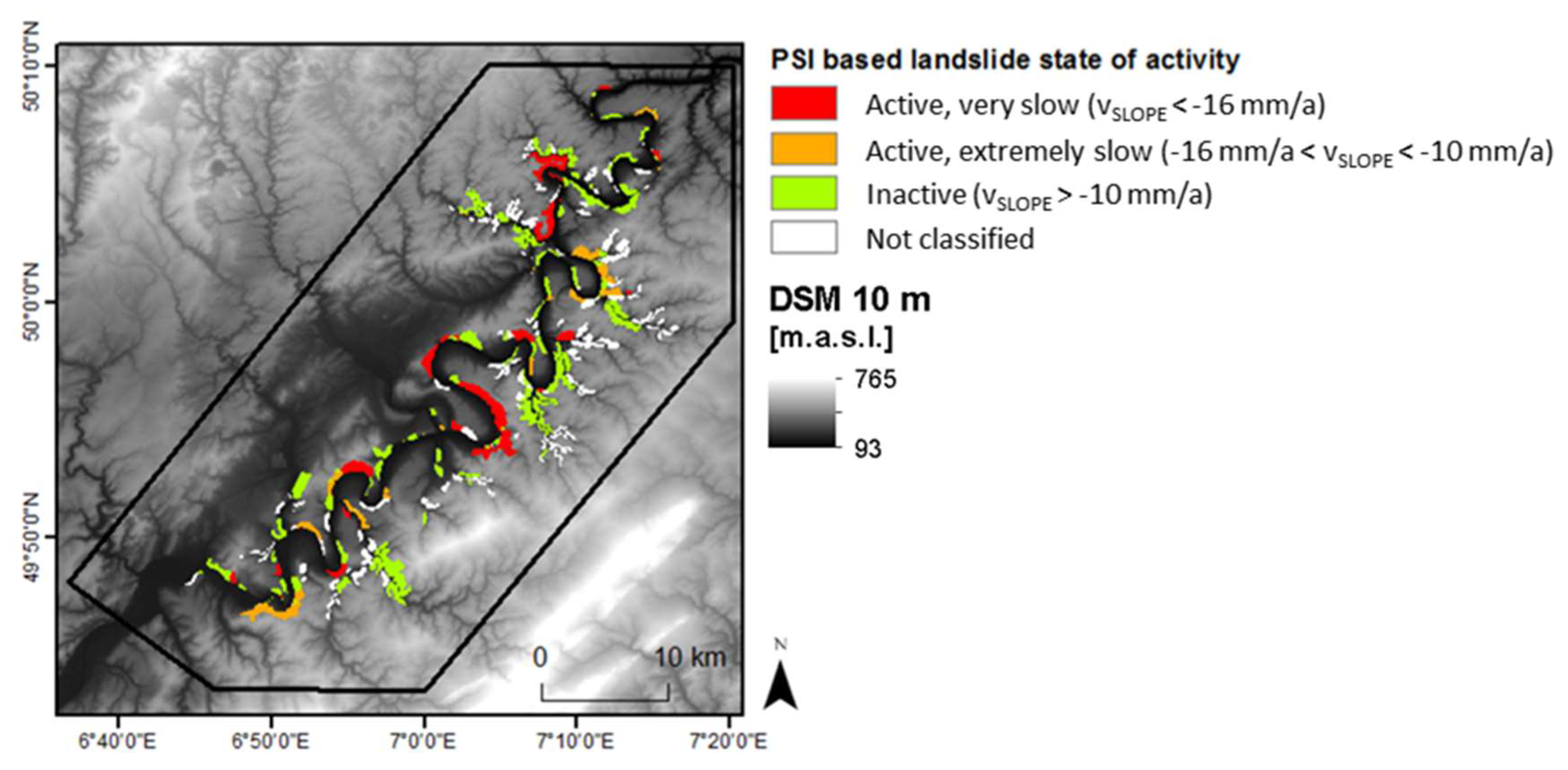
The result of the classification of the landslides’ state of activity is shown in Figure 5. The classification result consists of 23 “active, very slow” landslides, 24 “active, extremely slow”, 132 “inactive” landslides, and 204 “not classified” landslides. Thus, the landslides’ state of activity is classified for 46.7% of all a priori mapped landslides. 25% of all “verified sliding areas” are not intersecting with a PS cluster. The PS cluster distribution for each landslide hazard indication area shows that 74% of the PS clusters are located in potential sliding areas and rock-fall hazard areas. The other 26% of the PS clusters are located in verified and assumed sliding areas. The landslides classified as “active, very slow” and “active, extremely slow” are compared against “verified sliding areas” based on the landslide hazard indication map. The comparison shows a good correlation, and thus confirms the plausibility of the result (Figure 6). All large “verified sliding areas” have been successfully classified as active landslides. In addition, the PSI-based classification has classified several large areas mapped as a “potential sliding area” in the landslide hazard indication map (Figure 2) as “active, very slow” or “active, extremely slow”, such as in the southern and the northern part of the study area (white arrows in Figure 6).

5. Discussion

In this work, two PSI post-processing steps were performed in order to classify active and inactive landslides on a regional scale. These steps were performed with the intention to adapt the PSI processing results to the specific requirements for the routine monitoring of a priori known areas with a landslide hazard indication. Certain characteristics and limitations were associated with the post-processing steps, which are discussed as follows.

First, the LOS velocity was converted to the slope direction based on the assumption that the landslide motion is purely parallel to the slope direction. This is plausible for things like planar slides, but not for rotational slides, where a significant vertical motion component at the top of the slide can be present. In such a case, the v_SLOPE is overestimating the real velocity in slope direction, because a vertical velocity component is present. The second issue regarding LOS conversion is the overestimation of the slope velocity in areas with low sensitivity. These are slopes with an exposition approximately to the North or to the South, or slopes with an inclination perpendicular to the SAR incidence angle. In order to mitigate this effect, the C-Index was fixed to −0.3 if −0.3 ≤ C < 0 and to +0.3 if 0 ≤ C ≤ +0.3, as proposed by [28]. The consequence of this is that the velocity in slope direction cannot be higher than 3.33 times the LOS velocity. The third issue regarding the LOS conversion is that any noise in the LOS velocity is amplified by the conversion. Thus, a high measurement precision of the PSI processing results is a precondition for the conversion.

If multiple-PSI dataset with different observation geometries is available, such as from an ascending and descending orbit, the projection into slope direction could be improved. This could be achieved by estimating the vertical and the horizontal velocity vectors based on ascending and descending LOS observations. The estimated vertical velocity can then be used to improve the approximation of the velocity vector in the slope direction.

Detection of a PS cluster was performed to only classify landslides with a strong indication of a downslope motion as active. The rationale behind this approach was that the motion of a single PS could be due to a local process, such as building settlement. If several adjacent PSs showed a downslope motion, a strong indication regarding an active landslide is present. The drawback of the clustering approach is reduced classification completeness, as landslides with only one PS or heterogeneous v_SLOPE values are not classified. When two or more PS clusters with significantly different velocities are present in one landslide area, the extraction of one single velocity can be inappropriate. In such cases, a segmentation of the landslide area into two or more areas with different deformation characteristics can be performed [8].

Regarding the LOS velocity threshold to classify active landslides, recent studies have used thresholds in the range of 1.5 to 10 mm per year (e.g., [8,33,34,35,38]). In this work, a v_SLOPE threshold of 10 mm per year was used. This threshold was chosen because the LOS velocity was converted into the slope direction, causing an amplification of the noise of the LOS data and potential exaggeration of the v_SLOPE in areas with low sensitivity (e.g., North- and South-facing slopes). Another approach regarding the choice of a velocity threshold is the use of training data. If such data are available from field surveys or in situ measurements, the PSI velocity threshold can be determined by the highest number of agreements between the PSI-based activity classification and field-based observations.

A general limitation regarding the use of PSI to detect landslide displacements is the lack of PSs in the landslide area. The main reason for the lack of PSs is there being no geometrical visibility due to the local topography and LOS orientation, vegetation cover, and fast movements.

The geometrical visibility of a slope is a function of its exposition and slope angle, with respect to the SAR acquisition geometry. Due to foreshortening, layover and shadowing the amount of PSs can be significantly reduced. The use of SAR acquisitions taken from different orbits at different incidence angles increases the potential of high geometrical visibility.

A dense vegetation cover significantly limits the amount of PSs, because it causes a temporal decorrelation of the interferometric phase. If the phase decorrelation exceeds a certain threshold, no information is left, and the interferometric phase becomes random. Through the installation of corner reflectors or active transponders, the number of PSs in vegetated or agricultural areas can be increased (Figure 3B). Obviously, corner reflectors or active transponders cannot overcome the lack of PSs in archived SAR datasets, because the detection of PSs at corner-reflector or active-transponder sites can be achieved only after their installation.

The detection of PSs is limited for fast-moving landslides, due to an aliasing effect caused by the ambiguity of the interferometric phase. Therefore, the upper velocity limit of PSI is a quarter of a wavelength between two successive acquisitions. The time interval between two successive acquisitions is given by the satellite revisit time. Considering revisit time and wavelength, the maximum detectable velocities are 14.7 cm per year for ERS/Envisat (C band), 42.6 cm per year for Sentinel-1 12 day image pairs (C band), 25.7 cm per year for TerraSAR-X (X band), and 46.8 cm per year for ALOS (L band) [43]. These are theoretical values, but in practice, the ability to detect fast displacements depends on various aspects, such as the noise level of the data, the specific phase-unwrapping technique, the spatial pattern of the deformation phenomena (the smoother the pattern, the better), and the PS density over this phenomena (the higher the density, the better) [43,44]. Besides aliasing, another limitation of SAR interferometric methods is encountered when the strain rate reaches half a wavelength per resolution cell in the time consecutive observations [45]. The use of other SAR processing techniques, such as SAR feature tracking [46] or range split spectrum interferometry [47] to detect fast-moving landslides, could extend the detectable velocity range of the PSI technique. However, these techniques provide spatial resolutions and accuracies which are approximately one order of magnitude worse than advanced DInSAR techniques, which limits their applicability to fast and large landslides.

6. Conclusions

This work presented a PSI post-processing workflow for the classification of landslides’ states of activity on a regional scale. A PS cluster was proposed as a precondition for the classification of the landslide activity. The PSI dataset was verified by GPS measurements and showed a high correlation (mean difference: 0.49 mm per year). This result shows the operational readiness of the Sentinel-1 SAR mission to detect landslide displacements. Sentinel-1 is of particular interest, because there are several recently ongoing efforts are regarding the buildup of nationwide ground motion services based on this SAR mission, such as in [48,49,50].

The classification result consisted of 23 “active, very slow” landslides, 24 “active, extremely slow”, 132 “inactive” landslides, and 204 “not classified” landslides. The landslides classified as “active, very slow” and “active, extremely slow” were compared against “verified sliding areas” based on a landslide hazard indication map, and results show a good correlation (Figure 6). Furthermore, several “potential sliding areas” (mapped in the landslide hazard indication map) were classified as “active landslides” (based on PSI data), and public authorities could use this information to extend the monitoring efforts by installation of in-situ sensors for comprehensive monitoring on a local scale, or field surveys in these areas (e.g., areas marked with white arrows in Figure 6).

After verification by field surveys, the updated landslide inventory can enhance landslide susceptibility assessments, which can then be used for a landslide risk analysis and risk management, in order to improve DRR. A paradigm change regarding the use of advanced DInSAR techniques from single retrospective data products, to joint analysis of multiple SAR datasets from different SAR sensors covering consecutive timespans [8,14], towards a monitoring technique with continuously updated displacement information feeding a database [51] based on a single SAR mission, shows the increasing capability of advanced DInSAR techniques. This capability can be used to routinely produce classifications of landslides’ states of activity for an improved DRR. The use of (semi-) automated workflows for updating landslide inventories is of particular interest in the context of nationwide, advanced DInSAR datasets with millions of measurement points. Manual data analysis and visual interpretation makes the process subjective and time-consuming. The automatization and implementation of the proposed workflow within the framework of the BBD is under discussion.

References

- Cruden, D.M. A simple definition of a landslide. Bull. Int. Assoc. Eng. Geol. 1991, 43, 27–29. [Google Scholar] [CrossRef]
- Cruden, D.M.; Varnes, D.J. Landslide types and processes. In Landslides Investigation and Mitigation; Turner, A.K., Schuster, R.L., Eds.; Special Report 247; Transportation Research Board, US National Research Council: Washington, DC, USA, 1996; pp. 36–75. [Google Scholar]
- Froude, M.J.; Petley, D.N. Global fatal landslide occurrence from 2004 to 2016. Nat. Hazards Earth Syst. Sci. 2018, 18, 2161–2181. [Google Scholar] [CrossRef]
- Herrera, G.; Mateos, R.M.; García-Davalillo, J.C.; Grandjean, G.; Poyiadji, E.; Maftei, R.; Filipciuc, T.-C.; Jemec Auflič, M.; Jež, J.; Podolszki, L.; et al. Landslide databases in the Geological Surveys of Europe. Landslides 2018, 15, 359–379. [Google Scholar] [CrossRef]
- Gariano, S.L.; Guzzetti, F. Landslides in a changing climate. Earth-Sci. Rev. 2016, 162, 227–252. [Google Scholar] [CrossRef]
- Sassa, K.F.H.; Wang, F.; Wang, G. Landslides—Risk Analysis and Sustainable Disaster Management; Springer: Berlin, Germany, 2005; Volume 1. [Google Scholar]
- Guzzetti, F.; Mondini, A.C.; Cardinali, M.; Fiorucci, F.; Santangelo, M.; Chang, K.-T. Landslide inventory maps: New tools for an old problem. Earth-Sci. Rev. 2012, 112, 42–66. [Google Scholar] [CrossRef]
- Righini, G.; Pancioli, V.; Casagli, N. Updating landslide inventory maps using persistent scatterer interferometry (PSI). Int. J. Remote Sens. 2012, 33, 2068–2096. [Google Scholar] [CrossRef]
- Casagli, N.; Cigna, F.; Bianchini, S.; Hölbling, D.; Füreder, P.; Righini, G.; Del Conte, S.; Friedl, B.; Schneiderbauer, S.; Iasio, C.; et al. Landslide mapping and monitoring by using radar and optical remote sensing: Examples from the EC-FP7 project safer. Remote Sens. Appl. Soc. Environ. 2016, 4, 92–108. [Google Scholar] [CrossRef]
- Rosi, A.; Tofani, V.; Tanteri, L.; Tacconi Stefanelli, C.; Agostini, A.; Catani, F.; Casagli, N. The new landslide inventory of Tuscany (Italy) updated with PS-InSAR: Geomorphological features and landslide distribution. Landslides 2017, 15, 5–19. [Google Scholar] [CrossRef]
- Ferretti, A.; Prati, C.; Rocca, F. Permanent scatterers in sar interferometry. IEEE Trans. Geosci. Remote Sens. 2001, 39, 8–20. [Google Scholar] [CrossRef]
- Berardino, P.; Fornaro, G.; Lanari, R.; Sansosti, E. A new algorithm for surface deformation monitoring based on small baseline differential sar interferograms. IEEE Trans. Geosci. Remote Sens. 2002, 40, 2375–2383. [Google Scholar] [CrossRef]
- Ferretti, A.; Fumagalli, A.; Novali, F.; Prati, C.; Rocca, F.; Rucci, A. A new algorithm for processing interferometric data-stacks: Squeesar. IEEE Trans. Geosci. Remote Sens. 2011, 49, 3460–3470. [Google Scholar] [CrossRef]
- Cigna, F.; Bianchini, S.; Casagli, N. How to assess landslide activity and intensity with persistent scatterer interferometry (PSI): The PSI-based matrix approach. Landslides 2013, 10, 267–283. [Google Scholar] [CrossRef] [Green Version]
- Lu, P.; Casagli, N.; Catani, F.; Tofani, V. Persistent scatterers interferometry hotspot and cluster analysis (PSI-HCA) for detection of extremely slow-moving landslides. Int. J. Remote Sens. 2012, 33, 466–489. [Google Scholar] [CrossRef]
- Xi, F. Detektion von Anormalen Zeitreihen an Persistent-Scatterer-Punkten im Zusammenhang mit der Ableitung Flächenhafter Bodenbewegungen. Doctoral Thesis, TU Clausthal, Clausthal-Zellerfeld, Germany, 2017. [Google Scholar]
- LGB. Geologische Übersichtskarte von Rheinland-Pfalz 1:300,000; State Office of Geology and Mining Rhineland-Palatinate: Mainz, Germany, 2003. [Google Scholar]
- Zitzmann, A. The geological map of germany 1:200,000—From analogous sheets to a geological data bank. Z. Dtsch. Geol. Ges. 2003, 154, 121–139. [Google Scholar] [CrossRef]
- BKG. Digitales Geländemodell Gitterweite 10 m, dgm10. Product Description. Available online: http://www.geodatenzentrum.de/docpdf/dgm10.pdf (accessed on 16 November 2018).
- Krauter, E. Phänomenologie natürlicher böschungen (hänge) und ihrer massenbewegungen. In Grundbau-Taschenbuch, 1st ed.; Smoltczyk, U., Ed.; Ernst & Sohn: Berlin, Germany, 2001; Volume 6, pp. 613–666. [Google Scholar]
- Adam, N.; Kampes, B.; Eineder, M. Development of a scientific permanent scatterer system: Modifications for mixed ERS/ENVISAT time series. In Proceedings of the Envisat Symposium 2004, Salzburg, Austria, 6–10 September 2004; ESA: Paris, France, 2004. [Google Scholar]
- Goel, K.; Adam, N.; Shau, R.; Rodriguez-Gonzalez, F. Improving the reference network in wide-area persistent scatterer interferometry for non-urban areas. In Proceedings of the 2016 IEEE International Geoscience and Remote Sensing Symposium (IGARSS), Beijing, China, 10–15 July 2016; pp. 1448–1451. [Google Scholar]
- Rodriguez Gonzalez, F.; Bhutani, A.; Adam, N. L1 network inversion for robust outlier rejection in persistent scatterer interferometry. In Proceedings of the 2011 IEEE International Geoscience and Remote Sensing Symposium, Vancouver, BC, Canada, 24–29 July 2011; pp. 75–78. [Google Scholar]
- Adam, N. PSI-Prozessierung von Sentinel-1 Daten für den Bodenbewegungsdienst Deutschland: Erweiterungen des Integrierten Wide-Area Prozessors (IWAP) des DLR und Eigenschaften der erzeugten Produkte; BBD Workshop: Hannover, Germany, 2018. [Google Scholar]
- Wendleder, A.; Felbier, A.; Wessel, B.; Huber, M.; Roth, A. A method to estimate long-wave height errors of srtm c-band dem. IEEE Geosci. Remote Sens. Lett. 2016, 13, 696–700. [Google Scholar] [CrossRef]
- Notti, D.; Meisinia, C.; Zucca, F.; Colombo, A. Models to predict persistent scatterers data distribution and their capacity to register movement along the slope. In Proceedings of the Fringe Workshop 2011, Frascati, Italy, 19–23 September 2011. [Google Scholar]
- Notti, D.; Herrera, G.; Bianchini, S.; Meisina, C.; García-Davalillo, J.C.; Zucca, F. A methodology for improving landslide psi data analysis. Int. J. Remote Sens. 2014, 35, 2186–2214. [Google Scholar]
- Herrera, G.; Gutiérrez, F.; García-Davalillo, J.C.; Guerrero, J.; Notti, D.; Galve, J.P.; Fernández-Merodo, J.A.; Cooksley, G. Multi-sensor advanced DInSAR monitoring of very slow landslides: The Tena Valley case study (Central Spanish Pyrenees). Remote Sens. Environ. 2013, 128, 31–43. [Google Scholar] [CrossRef]
- Anselin, L. Local indicators of spatial association—Lisa. Geogr. Anal. 1995, 27, 93–115. [Google Scholar] [CrossRef]
- Ketelaar, V.B.H.G. Satellite Radar Interferometry—Subsidence Monitoring Techniques, 1st ed.; Springer: Berlin, Germany, 2009; p. 244. [Google Scholar]
- Adam, N. The development of a high precision troposphere effect mitigation processor for SAR interferometry. In Proceedings of the IGARSS 2018, Valencia, Spain, 22–27 July 2018; pp. 1–4. [Google Scholar]
- Cruden, D. A suggested method for describing the rate of movement of a landslide. Bull. Int. Assoc. Eng. Geol. 1995, 52, 75–78. [Google Scholar]
- Farina, P.; Colombo, D.; Fumagalli, A.; Marks, F.; Moretti, S. Permanent scatterers for landslide investigations: outcomes from the ESA-SLAM project. Eng. Geol. 2006, 88, 200–217. [Google Scholar] [CrossRef]
- Cascini, L.; Fornaro, G.; Peduto, D. Advanced low- and full-resolution DInSAR map generation for slow-moving landslide analysis at different scales. Eng. Geol. 2010, 112, 29–42. [Google Scholar] [CrossRef]
- Bianchini, S.; Solari, L.; Casagli, N. A gis-based procedure for landslide intensity evaluation and specific risk analysis supported by persistent scatterers interferometry (PSI). Remote Sens. 2017, 9, 1093. [Google Scholar] [CrossRef]
- Mansour, M.F.; Morgenstern, N.R.; Martin, C.D. Expected damage from displacement of slow-moving slides. Landslides 2011, 8, 117–131. [Google Scholar] [CrossRef]
- Bianchini, S.; Herrera, G.; Mateos, R.; Notti, D.; Garcia, I.; Mora, O.; Moretti, S. Landslide activity maps generation by means of persistent scatterer interferometry. Remote Sens. 2013, 5, 6198–6222. [Google Scholar] [CrossRef]
- Bianchini, S.; Cigna, F.; Righini, G.; Proietti, C.; Casagli, N. Landslide hotspot mapping by means of persistent scatterer interferometry. Environ. Earth Sci. 2012, 67, 1155–1172. [Google Scholar] [CrossRef]
- Rodriguez Gonzalez, F.P.A.; Fuh Chuo, E.; Brcic, R.; Shau, R.; Adam, N.; Redl, S.; Siegmund, R. Processing Report for the Ground Motion Service Germany; DLR: Oberpfaffenhofen, Germany, 2017; p. 627. [Google Scholar]
- LBM. Auswertung der Corner Reflektor Messung vom 14.06.2018; Landesbetrieb Mobilität Rheinland-Pfalz: Trier, Germany, 2018. [Google Scholar]
- Rogall, M. Gefahrenhinweiskarte Mittelmosel—Rutschungen und Steinschläge 1:50.000 Erläuterungen; State Office of Geology and Mining Rhineland-Palatinate: Mainz, Germany, 2014; p. 32. [Google Scholar]
- Riedmann, M.; Lang, O.; Bindrich, M. Terrasar-x basierte Hangrutschüberwachung bei Graach Rheinland-Pfalz. In GeoMonitoring 2015; Wolfgang, B., Steffen, K., Eds.; Clausthal-Zellerfeld, Germany, 2015; p. 250. Available online: http://www.geo-monitoring.org/Tagung2015/Tagungsband_inh_2015.pdf (accessed on 16 November 2018).
- Crosetto, M.; Monserrat, O.; Cuevas-González, M.; Devanthéry, N.; Crippa, B. Persistent scatterer interferometry: A review. ISPRS J. Photogramm. Remote Sens. 2015, 115, 78–89. [Google Scholar] [CrossRef]
- Van Leijen, F. Persistent Scatterer Interferometry Based on Geodetic Estimation Theory. Ph.D. Thesis, TU Delft, Institutional Repository, Delft, Netherlands, 2014. [Google Scholar]
- Rosen, P.A.; Hensley, S.; Joughin, I.R.; Li, F.K.; Madsen, S.N.; Rodriguez, E.; Goldstein, R.M. Synthetic aperture radar interferometry. Proc. IEEE 2000, 88, 333–382. [Google Scholar] [CrossRef] [Green Version]
- Werner, C.; Strozzil, T.; Wiesmann, A.; Wegmuller, U.; Murray, T.; Pritchard, H.; Luckman, A. Complimentary measurement of geophysical deformation using repeat-pass SAR. In Proceedings of the IGARSS 2001, Scanning the Present and Resolving the Future, IEEE 2001 International Geoscience and Remote Sensing Symposium (Cat. No. 01CH37217), Sydney, NSW, Australia, 9–13 July 2001; Volume 3257, pp. 3255–3258. [Google Scholar]
- Shi, X.; Jiang, H.; Zhang, L.; Liao, M. Landslide displacement monitoring with split-bandwidth interferometry: A case study of the shuping landslide in the three gorges area. Remote Sens. 2017, 9, 937. [Google Scholar] [CrossRef]
- Dehls, J. InSAR.No: A national insar deformation mapping service in Norway. In Proceedings of the Fringe 2017—10th International Workshop on Advances in the Science and Applications of SAR Interferometry and Sentinel-1 InSAR, Helsinki, Finnland, 5–9 June 2017. [Google Scholar]
- Oyen, A. Towards an insar based nationwide monitoring strategy in the Netherlands. In Proceedings of the Fringe 2017—10th International Workshop on Advances in the Science and Applications of SAR Interferometry and Sentinel-1 InSAR, Helsinki, Finnland, 5–9 June 2017. [Google Scholar]
- Kalia, A.C.; Frei, M.; Lege, T. A copernicus downstream-service for the nationwide monitoring of surface displacements in Germany. Remote Sens. Environ. 2017, 202, 234–249. [Google Scholar] [CrossRef]
- Raspini, F.; Bianchini, S.; Ciampalini, A.; Del Soldato, M.; Solari, L.; Novali, F.; Del Conte, S.; Rucci, A.; Ferretti, A.; Casagli, N. Continuous, semi-automatic monitoring of ground deformation using Sentinel-1 satellites. Sci. Rep. 2018, 8, 7253. [Google Scholar] [CrossRef] [PubMed]
Figure 1.
(A) Geological setting (modified from geological map 1:200,000, GK1000, © BGR, Hannover, 2018 [18]). (B) Elevation map of the study area, based on a Digital Elevation Model (DEM) © GeoBasis-DE/BKG 2018 [19] and characteristic elevation transect across the river Moselle. The location of the transect is indicated by the blue line. (C) Location of the study area (red polygon) in Germany.
Figure 2.
(A) Landslide hazard indication map (modified after [41]). The boundary of the study area is shown by the black outline. A DEM © GeoBasis-DE/BKG 2018 [19] serves as background. (B) The terrain aspect of all the sliding areas mapped in the landslide hazard indication map. East corresponds to 90 degrees, West corresponds to 270 degrees.
Figure 3.
(A) Overview of the spatial distribution of the persistent scatterers (PSs) in the study area. (B,C) shows the location of the corner reflectors used for verification of the Sentinel-1 Persistent Scatterer Interferometry (PSI) data. (D) Shows the result of the verification of the Sentinel-1 PSI Line-of-Sight (LOS) velocity, versus the Global Positioning System (GPS) velocity at the corner reflector sites.
Figure 4.
(A,D) visualize the Sentinel-1 PSI mean velocity in the LOS direction. (B,E) show the results of the conversion in a slope direction. PSs indicating uphill motion and PSs in flat areas are discarded. (C,F) show the results of the PS cluster analysis. The location of (A–C) is indicated in Figure 3A, number 1. The location of (D–F) is indicated in Figure 3A, number 2. A DEM © GeoBasis-DE/BKG 2018 [19] serves as background.
Figure 5.
Result of the classification of the landslide state of activity based on Sentinel-1 PSI data. A DEM © GeoBasis-DE/BKG 2018 [19] serves as background.
Figure 6.
Verification of the classification result regarding “active landslides” (A) with “verified sliding areas” from the landslide hazard indication map (B). A DEM © GeoBasis-DE/BKG 2018 [19] serves as background.
© 2018 by the author. Licensee MDPI, Basel, Switzerland. This article is an open access article distributed under the terms and conditions of the Creative Commons Attribution (CC BY) license (http://creativecommons.org/licenses/by/4.0/).
Share and Cite
MDPI and ACS Style
Kalia, A.C. Classification of Landslide Activity on a Regional Scale Using Persistent Scatterer Interferometry at the Moselle Valley (Germany). Remote Sens. 2018, 10, 1880. https://doi.org/10.3390/rs10121880
AMA Style
Kalia AC. Classification of Landslide Activity on a Regional Scale Using Persistent Scatterer Interferometry at the Moselle Valley (Germany). Remote Sensing. 2018; 10(12):1880. https://doi.org/10.3390/rs10121880
Chicago/Turabian StyleKalia, Andre Cahyadi. 2018. "Classification of Landslide Activity on a Regional Scale Using Persistent Scatterer Interferometry at the Moselle Valley (Germany)" Remote Sensing 10, no. 12: 1880. https://doi.org/10.3390/rs10121880
Note that from the first issue of 2016, this journal uses article numbers instead of page numbers. See further details here.