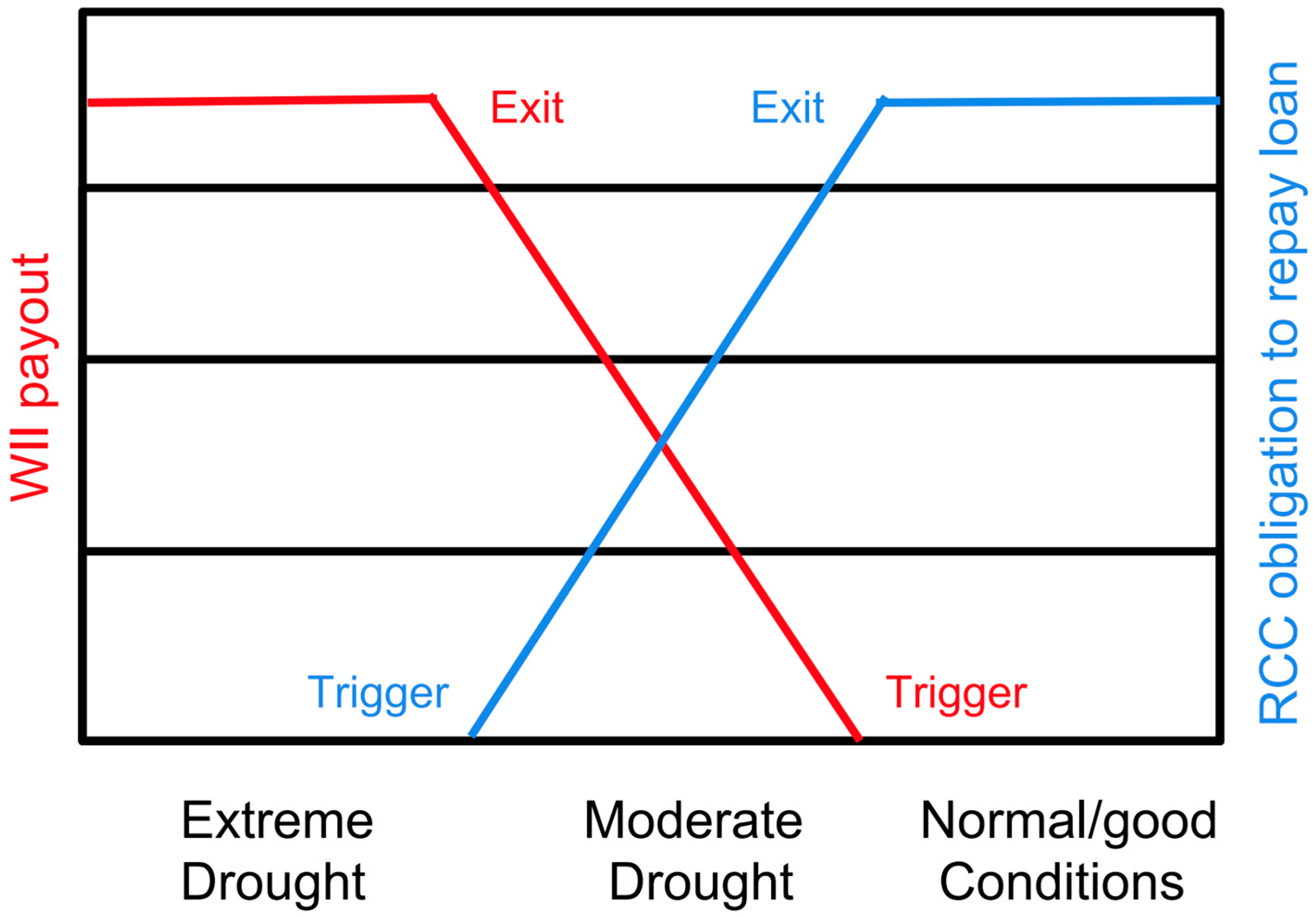
Article

What Rainfall Does Not Tell Us—Enhancing Financial Instruments with Satellite-Derived Soil Moisture and Evaporative Stress

1
International Research Institute for Climate and Society, Columbia University, New York, NY 10964, USA
2
CDMX—Research Center for Sustainable Development, Mexico City 10200, Mexico
3
NASA Marshall Space Flight Center, Earth Science Branch, Huntsville, AL 35812, USA
4
Earth System Science Center, University of Alabama in Huntsville, Huntsville, AL 35899, USA
5
Hydrology and Remote Sensing Laboratory, Agricultural Research Service, United States Department of Agriculture, Beltsville, MD 20705, USA
6
International Food Policy Research Institute, Washington, DC 20005, USA
7
Macro Agriculture Research Institute, College of Economics and Management, Huazhong Agricultural University, Wuhan 430070, Hubei, China
8
Department of Geodesy and Geoinformation, Vienna University of Technology, 1040 Vienna, Austria
*
Author to whom correspondence should be addressed.
Remote Sens. 2018, 10(11), 1819; https://doi.org/10.3390/rs10111819
Submission received: 29 August 2018 / Revised: 22 October 2018 / Accepted: 13 November 2018 / Published: 16 November 2018

Abstract

:
Advanced parametric financial instruments, like weather index insurance (WII) and risk contingency credit (RCC), support disaster-risk management and reduction in the world’s most disaster-prone regions. Simultaneously, satellite data that are capable of cross-checking rainfall estimates, the “standard dataset” to develop such financial safety nets, are gaining importance as complementary sources of information. This study concentrates on the analysis of satellite-derived multi-sensor soil moisture (ESA CCI, Version v04.2), the evapotranspiration-based Evaporative Stress Index (ESI), and CHIRPS (Climate Hazards Group InfraRed Precipitation with Station data) rainfall estimates in nine East African countries. Based on spatial correlation analysis, we found matching spatial/temporal patterns between all three datasets, with the highest correlation coefficient occurring between October and March. In large parts of Kenya, Ethiopia, and Somalia, we observed a lower (partly negative) correlation coefficient between June and August, which was likely caused by issues related to cloud cover and the volume scattering of microwaves in sandy, hot soils. Based on simple linear and logit regression analysis with annual, national maize yield estimates as the dependent variable, we found that, depending on the chosen period (averages per year, growing or harvesting months), there was added value (higher R-squared) if two or all three variables were combined. The ESI and soil moisture have the potential to close sensitive knowledge gaps between atmospheric moisture supply and the response of the land surface in operational parametric insurance projects. For the development and calibration of WII and RCC, this means that better proxies for historical and potential future drought impact can strengthen “drought narratives”, resulting in a better match between calculated payouts/credit repayment levels and the actual needs of smallholder farmers.

1. Introduction

Approximately 2.5 billion full- or part-time smallholder farmers are managing the world’s estimated 500 million farms [1]. In low-income countries, farmers often mention weather shocks as their greatest concern [2]. Extreme climate events can affect their agricultural production in two ways: directly, through biophysical impact on agricultural production, and indirectly, by affecting risk perception and related agricultural management decisions. Parametric insurance approaches and global partnerships like Insuresilience (https://www.insuresilience.org/) aim to cover 400 million vulnerable people in low-income countries. These programs try to complement progress in agricultural management with financial instruments [3], encouraging farmers to invest in measures that better exploit their agricultural potential with the help of a financial safety net [4]. Ideally, these financial instruments also strengthen the disaster resilience of smallholder farmers, for instance through food reserves and access to loans or by lowering the barrier to invest in drought-resistant seeds. In this way, index insurance has the potential to contribute directly or indirectly to sustainable development by closing sensitive gaps in the existing climate risk-management portfolio [3].
Traditionally, many agricultural insurance programs were based on in situ measurements of precipitation. However, weather-station data are not the most reliable source of information for designing index insurance programs on the African continent. Not only do they require regular maintenance, but, in many African countries, the density of weather stations is insufficient and the distribution uneven [5]. During the last decade, satellite-based estimation of moisture-related parameters, collectively capable of closing the critical gap between rainfall deficits and the response of the land surface, has reached a level of maturity that warrants integration into a host of applications [6,7]. Different satellite-derived estimates of soil moisture and evapotranspiration (ET) are available as operational datasets. Soil moisture, for instance, has been used to validate or complement satellite-based rainfall estimates [8]. Since the basic mechanism of parametric drought insurance to trigger payouts is not linked to crop loss but to thresholds in variables representing critical moisture or vegetation health conditions during predefined windows in the agricultural season, weather insurance indices require input datasets that can robustly capture drought conditions both spatially and temporally.
This study concentrates on analyzing the performance of satellite-derived precipitation, soil moisture. and evapotranspiration in the context of WII and RCC, two approaches toward parametric insurance. Since there are already more than 50 different drought indicators and indices [9], the overall objective is not to develop yet another, but to focus on three complementary tasks:
(1) to analyze the spatiotemporal correlation of satellite-derived precipitation, soil moisture, and evapotranspiration to better understand the connections between moisture deficits and the response of the land surface in nine East African countries (Burundi, Djibouti, Eritrea, Ethiopia, Kenya, Rwanda, Somalia, Uganda, and the United Republic of Tanzania); (2) to run regression analysis with reported maize yield as the dependent variable to statistically capture the relationship between the three satellite datasets and agricultural production; and (3) to foster the mutual understanding between Earth observation and the insurance community, which has so far been a major limitation for the adoption of Earth observation datasets in insurance programs [10].
The guiding principle is that a more accurate representation of the hydrologic cycle beyond rainfall estimates can improve our characterization of the complex environmental root causes behind agricultural drought impacts. These root causes are centered on moisture deficits, which can be caused by insufficient (atmospheric) moisture supply, increased evapotranspiration, or both. From a remote-sensing perspective, this means that basis risk, defined as the mismatch between satellite data-driven parameterized insurance models and farmer requirements on the ground [9,10,11], can be reduced if we manage to strengthen event-specific narratives with independent satellite-derived estimates such as soil moisture or evapotranspiration.
In Section 2, we discuss the specific role of satellite-derived soil moisture and evapotranspiration estimates for parametric insurance. Section 3 describes the region of interest with regard to land cover, agroecological zones, and topography. In Section 4, we focus on a more detailed description of the datasets and the methods used in this study. Results are discussed in Section 5, and Section 6 provides a summary of the overall findings in this study.

2. Role of Soil Moisture and Evapotranspiration for Parametric Insurance

Both WII and RCC try to increase the disaster resilience of vulnerable populations towards extreme climate events by decoupling payouts from expensive small-scale loss assessments, which is reflected in lower premiums paid by farmers and faster payouts in the case of WII. Premiums are paid either in cash or via alternative mechanisms like the insurance for assets scheme used by the R4 Rural Resilience Initiative (http://www1.wfp.org/r4-rural-resilience-initiative). WII payouts are usually linked to rainfall deficits [11] and/or proxies for vegetation health (e.g., the satellite-derived Normalized Difference Vegetation Index (NDVI)) during sensitive growing periods in the agricultural season. Starting at a predefined threshold value (the “trigger”), payouts increase linearly until the maximum payout (the “exit”) is reached. RCC basically inverts this model (Figure 1) to limit the risk of agricultural loan taking in drought-prone areas by establishing a parametric relationship between drought conditions and the obligation to return loans. Credit constraints are common among low-income farmers due to limited collateral, resulting in reduced access to seeds, fertilizer, etc. RCC tries to solve this problem by providing farmers with collateral-free loans [12] at relatively high interest rates to increase their productivity. More severe drought conditions result in partial offsetting of loan repayments, whereas the loan has to be repaid in full if no drought conditions were detected.
Satellite-derived soil moisture and evapotranspiration are relatively newly available remotely sensed variables. The hydrologic cycle causes a distinct feedback loop between rainfall and soil moisture, which is, by nature, very heterogeneous [13]. This feedback loop influences terrestrial water and energy cycles [14]. One main reason for this complexity is that the response of the atmosphere to changes in soil moisture is neither linear nor unidirectional [15]. Since more than half of the solar energy that is absorbed by the land surface is used to evaporate water [16], soil moisture, land-surface temperature and evapotranspiration are intrinsically linked [17].
Verstraeten et al. [18] state that “the proper assessment of evapotranspiration and soil-moisture content are fundamental to food-security research”. Remotely sensed soil moisture and evapotranspiration datasets exhibit complementary strengths and weaknesses because their retrieval is based on different sensors, retrieval mechanisms, and algorithmic approaches. Microwave-based soil-moisture remote-sensing techniques struggle with obtaining valid retrievals under dense vegetation because measurements are not only sensitive to the dielectric properties of water molecules in the soil (used to estimate soil moisture), but also to characteristics related to surface roughness, vegetation cover, and topography [19,20]. While high vegetation density is not problematic for the Evaporative Stress Index (ESI) [21], thermal infrared-based evapotranspiration estimates used in the ESI are strongly affected by cloud cover [22,23]. In contrast, microwave-based soil-moisture retrievals have all-sky capabilities.
By investigating factors influencing the performance and reliability of satellite-derived soil moisture and the ESI, as well as their agreement with reported maize yields, this study aims to pave the way for the next generation of satellite-based parametric insurance projects, moving beyond vegetation and precipitation indices to indicators more tightly tied to plant available moisture constraints. These projects rely on the cross-validation of different variables to increase confidence in the representation of drought conditions via satellite data [22].

3. Region of Interest

Figure 2 illustrates the land-cover types in the region of interest based on the latest (2012) classification from NASA’s Moderate Resolution Spectroradiometer (MCD12Q1), available via the Land Processes Distributed Active Archive Center (https://lpdaac.usgs.gov/dataset_discovery/modis/modis_products_table/mcd12q1) at a spatial resolution of 500 meters [24]. The classification distinguishes 17 land-cover classes defined by the International Geosphere Biosphere Program (IGBP), including 11 natural vegetation classes, three developed and mosaicked land classes, and three nonvegetated land classes. Grassland, shrubland, and barren land dominate the eastern part of the study region (the lowlands of Eritrea, Djibouti, Somalia, Ethiopia, and Kenya). The west of the study region (Ethiopian highlands, western parts of Kenya, Uganda, Rwanda, Burundi, and Tanzania) is mainly characterized by cropland, tree cover, and grassland. Not all cropland areas are exclusively planted with maize, but maize is the dominant crop in the study region.
Figure 3 shows the agroecological zones [25] contained within the study area, as well as the regional topography as represented by the 90 m Shuttle Radar Topography Mission (CIAT CSI SRTM version4p1) digital elevation model. There is a distinct west–east gradient from cool tropical zones (large parts of Rwanda, Burundi, Tanzania, and Western Kenya) and warm, humid zones (mainly Burundi) to (semi)arid warm zones (lowlands of Somalia, Kenya, Ethiopia, Djibouti, and Eritrea) and subhumid zones (large parts of Tanzania).

4. Datasets and Methods

4.1. Satellite Data

In addition to precipitation and temperature, soil moisture is listed as one of three essential climate variables (ECV) that are considered in all nine social benefit areas, ranging from agriculture over climate to disasters and health [26]. Until recently, evapotranspiration was not explicitly mentioned as an ECV, but indirectly acknowledged due to its close relationship with temperature, and water use and availability. In 2018, both the Terrestrial Observation Panel for Climate (TOPC) and the Global Climate Observing System (GCOS) listed evaporation as an ECV and therefore a high-priority Earth-observation parameter (https://board.geo.tuwien.ac.at/discussion/137/ecv-evaporation-from-land-sensible-heat-flux). Decrements of actual ET from potential values expected under well-watered conditions provide a metric of moisture deficiency and vegetative stress.
The analyses presented here use the multi-sensor soil-moisture dataset generated through the Climate Change Initiative of the European Space Agency (ESA CCI, Version v04.2) [26,27,28]. ESA CCI soil moisture is an offline dataset that is currently being transferred to an operational data service. ET-based drought indicators are becoming increasingly used as an early indicator of drought-induced crop stress. In this study, we focus on ESI generated through the Atmosphere Land Exchange Inverse (ALEXI) surface energy balance model, in its current form driven by thermal infrared retrievals of land-surface temperature [29,30]. The ESI describes anomalies in the ratio of actual to potential evapotranspiration, highlighting regions of lower-than-normal consumptive water use by crops and natural vegetation. Rainfall estimates are provided via the CHIRPS (Climate Hazards Group InfraRed Precipitation with Station data) dataset, a quasi-global rainfall dataset that is available from 1981 to the near present [31].

4.1.1. Satellite-Derived Soil Moisture

The ESA CCI surface soil-moisture dataset combines retrievals from thirteen active (radar) and passive (radiometer) sensors to generate a daily surface soil-moisture product at a spatial resolution of 0.25 degrees (roughly 28 km at the equator) [32]. While the blending scheme of previous versions was based on the use of radiometers for areas with low vegetation density, radars for regions with high vegetation density and their combination for areas with high agreement (R > 0.65), Version v04.2 includes a weighted blending scheme [32]. Since Version v03.2, the blending considers the highest-quality observations available during a certain period. A weighted average of estimates from all sensors is used to generate the final global product, whereas the blending weight for each dataset is calculated daily as the reciprocal of its random error variance [33]. The random errors of the final global datasets are lower than those of individual input datasets. Retrievals over areas with very dense vegetation, such as tropical forests, are generally not considered, because neither sensor type performs satisfactorily. East Africa is dominated by soil-moisture estimates from radiometers.
One major advantage of soil-moisture retrievals via radars or microwave radiometers is that they are largely independent from weather conditions (e.g., cloud cover). However, there are other physical limitations, such as penetration depth, which limit the ESA CCI dataset to a representation of soil moisture in the top layer (few centimeters) of the soil [34,35]. In addition, performance is degraded in regions of complex topography (e.g., mountainous terrain) and over frozen/snow-covered soils [36]. While soil-moisture retrieval algorithms have originally been applied to sensors designed for other purposes, they are now used to develop fully operational datasets and applied to dedicated soil-moisture sensors. The latest update of the ESA CCI soil-moisture dataset covers the years 1978–2016. It will be made available as an operational dataset with 10 daily updates in 2018. Compared to modeled soil moisture, the previous version of the ESA CCI dataset (V02.1) showed comparable wet and dry patterns, and particularly good results in Kenya [37].

4.1.2. ESI

The ESI [29,30] represents standardized anomalies in the ratio of actual-to-potential ET, (fRET = ET/RET), where ET is actual ET retrieved using the ALEXI two-source energy-balance algorithm [38] and RET is a reference ET computed using a Penman–Monteith formulation for grass [39]. Normalization by RET serves to minimize variability in ET due to seasonal variations in available energy and atmospheric demand, further refining focus on the soil-moisture signal. To highlight differences in moisture conditions between years, standardized anomalies in fRET are expressed as a pseudo z-score, normalized to a mean of zero and a standard deviation of one with respect to baseline fields describing “normal” (mean) conditions over the period of record. Extensive assessments of fRET and ESI in comparison with soil-moisture observations, standard drought indicators, and crop-yield datasets have shown the ability of land-surface temperature to act as a proxy for surface soil-moisture conditions and reflecting plant response to limiting soil-moisture availability [21,23,40,41,42].
Here, the ESI within ALEXI is generated from twice-daily estimates of LST from MODIS Terra from 2000 to the present over Africa at a spatial resolution of 0.05° using a time-differencing difference technique [43]. Satellite-based leaf area index (LAI) information needed by ALEXI for characterization of the vegetative canopy is taken from the NOAA LAI Climate Data Record [44]. Meteorological inputs including atmospheric profiles of potential temperature, specific humidity, and geopotential height and surface variables, such as air temperature, surface pressure, incoming solar radiation, and wind speed are taken from the Climate Forecast System Reanalysis [45] product. CFS-R provides data at three-hour analysis time steps with 1–6 forecasts in between analyses, effectively providing full three-dimensional atmospheric data at an hourly temporal resolution. The ALEXI model has been tested over East Africa and showed a high agreement with modelled soil-moisture datasets from the Noah land-surface model and the Land Parameter Retrieval Model (LPRM) [46,47]. While the MODIS LST product includes a cloud flag, residual cloud contamination can add noise to the thermal retrievals of ET particularly during times of persistent cloud cover. An all-sky microwave-based LST product, using observations in the Ka band, is being integrated into the ALEXI modeling system to reduce the impact of cloud contamination in thermal retrievals [48].

4.1.3. CHIRPS

The CHIRPS precipitation dataset merges satellite measurements with station observations to produce pentadal (five-daily) estimates of precipitation [31] at a spatial resolution of 0.05°. CHIRPS relies on cold cloud duration (CCD) for rainfall estimation. A subset of available station data are used to generate a preliminary dataset with a timeliness of three days. However, the final product with all available station data is available in the middle of the following month. Different studies confirmed the adequate performance of CHIRPS at capturing both spatial and temporal variability in rainfall as measured by independent station data [49,50]. CHIRPS has been optimized for drought-monitoring applications [31]. As typical for satellite-based rainfall estimates, retrieval issues (overestimation) have been identified in CHIRPS in high-lying complex terrain [51], along with a general tendency to underestimate rainfall variance [31]. With regard to the performance of CHIRPS in East Africa, Kimani et al. [52] observed an overestimation of strong rainfall events during the MAM season, which is very likely associated with deep convective systems resulting in increased rainfall amounts.

4.2. Maize Yield Estimates and Agricultural Calendar

Figure 4 illustrates annual maize yield statistics in hectograms per hectare (10,000 hectograms = 1 ton) from FAOSTAT (http://www.fao.org/faostat/en/#data) for all nine countries in the study area. Rwanda tripled its maize yield from 2000 to 2014, but faced a decrease to around 1.6 tons in 2015 and 2016. Maize yield in Ethiopia more than doubled, from 1.6 tons in 2000 to 3.6 tons in 2016. Overall, Eritrea showed the lowest levels of maize yield, averaging around 0.8 tons since 2004. The United Republic of Tanzania had the second highest overall yield in 2001 (nearly 3.2 tons), but a steady decrease resulted in yields of around 1.4 tons since 2004. Reports from the United States Agency for International Development [53] mentioned inadequate drought-relief interventions as a probable cause. Despite droughts, Kenya’s maize yield remained relatively stable, at around 1.6 tons, but decreased to 1.4 tons in 2016.
There are trends in maize data in East Africa. However, the underlying reasons are not only complex and potentially interrelated, but uncertain. Reasons range from policies affecting agricultural production to climate-attributable impacts and technological advancements. On the one hand, there are studies that predict a primarily negative impact of climate change on different crops, such as maize, in (East) Africa [54]. On the other hand, there is uncertainty as to what degree agricultural advancement can generally mitigate climate-change impact on agricultural production [55].
Regression analysis was carried out for annual averages of satellite-derived precipitation, soil moisture, and evapotranspiration, as well as for (sub)seasonal averages. In addition to annual averages, we averaged monthly values for growing and harvesting months in countries with uni- and bimodal rainfall regimes to reduce uncertainties related to which (part of the) rainy season affected changes in annual maize yield. Estimates for the sowing, growing, and harvesting months are provided by crop calendars from FAO’s Global Information and Early Warning System (http://www.fao.org/giews/en/) and the respective country briefs (Figure 5).

4.3. Methods

From a methodical perspective, this paper is divided into two parts: the first part concentrates on satellite data processing and spatiotemporal analysis (Section 4.3.1), and the second on regression analysis with annual maize yield statistics from FAOSTAT (Section 4.3.2).

4.3.1. Satellite Data Processing and Spatiotemporal Analyses

The main objective of spatiotemporal analysis, which analyzes both temporal and spatial effects on correlations, was to identify months or regions that show particularly high or low agreement between the satellite-derived soil moisture, and the ESI and CHIRPS datasets. In this way, it is possible to relate spatial (dis)agreement to known strengths and weaknesses in the satellite products. All three satellite products were resampled to the same 0.25 degree grid. While the soil-moisture data were already on a native 0.25 degree grid, the data points were not located at the same geolocations as the ESI data. Therefore, resampling of the soil-moisture dataset to the ESI grid was completed. The monthly 0.05 degree CHIRPS data was resampled to the 0.25 degree ESI grid by averaging the data over the larger grid. With the resampled data, the linear relationship between monthly soil moisture, ESI, and CHIRPS was quantified based on the Pearson’s correlation coefficient for every 0.25 degree data point (spatial correlation map). For regression analysis, we applied a mask (Figure 2) to all three satellite products to focus exclusively on pixels that were classified as “cropland”. From the masked data, national averages were then calculated.

4.3.2. Regression Analysis

Since maize yield data are available as annual estimates from FAOSTAT, regression analysis was carried out using annual as well as (sub)seasonal rainfall, soil moisture, and the ESI averages, masked for all land-cover classes except cropland. The first diagnosis is panel regression analysis with fixed effects, whereas the restriction to annual maize yield records makes it impossible to explicitly relate deficits in the first or second rainy season (in bimodal rainfall regimes) to changes in annual yield. By including country and year fixed effects in the model, we are controlling for any unobserved heterogeneity among countries that is constant over time. This approach aims to control for both initial differences in country-level characteristics that should not bias the estimators obtained in the regressions and time variations in yield. but is not applicable the log regression (i.e., not applicable to binary variables). However, it should be noted that conclusions about the added-value of individual or combined datasets for parametric insurance are primarily derived from relative changes in regression coefficients rather than absolute values.
Linear regression estimates the change in a dependent continuous variable given the variation of a continuous independent variable. In this case, we are estimating the impact of the three moisture-related variables on agricultural yield in the eight focus countries of this study. The ninth country, Djibouti, is missing due to lack of pixels classified as cropland in MODIS MCD12Q1. All regression analyses were carried out based on standardized monthly anomalies (Equation (1)) of precipitation, soil moisture, and the ESI to minimize the effect of different value ranges in the three datasets on the overall results.
Z = (X − μ)/σ
where Z = standardized anomaly, X = monthly average, μ = mean, σ = standard deviation.
The second diagnosis is a logit regression to estimate the impact of rainfall, soil moisture, and evaporative stress on extreme yield outcomes. The logit model estimates change in the probability of a binary outcome variable given the variation of a continuous independent variable. We generated a binary variable (Equation (2)) that reflects yield levels based on a ranking of yield data in each country.
B a d Y e a r i , t = { 1 ,    i f   x t   i s   o n e   o f   b o t t o m   3   y e a r s   i n   c o u n t r y   i 0 ,    o t h e r w i s e
where B a d Y e a r i , t is the newly created binary variable in country i in year t, and x t is the yield value in t.
The three years with the lowest yield were set as 1, all others to 0. We chose three years to focus on the extremes, represented by the worst 19 percent of observations. This new binary “bad year” variable allows estimating the change in the probability of observing a bad year, given a variation in climate conditions as characterized by the three satellite variables (individual and combined). This kind of binary screening of good versus bad (most likely drought impact) years is more in line with the processes used to develop and calibrate insurance indices.

5. Results

5.1. Spatial Correlation Analysis

The results of the correlation analysis indicate both a temporal and a spatial pattern (Figure 6). Overall, the correlation coefficient tends to be higher between October and March than in the summer months of the Northern Hemisphere for all correlated pairs. This pattern is very likely related to increased cloud cover in the summer months, which affects the interaction of space-based sensors with the land surface. The average correlation coefficient of ESI vs. soil moisture is slightly higher than CHIRPS vs. ESI (both around 0.4) and CHIRPS vs. SM (0.35). Our results indicate that all three satellite-derived datasets can generally be regarded as cascading sources of information, but neither in all countries, nor during all months. This is in line with other studies, which, based on ground stations and satellite datasets, suggest both positive and negative feedback loops between all three variables, but also positive correlations between evapotranspiration and soil moisture as well as evapotranspiration and rainfall in East Africa [14]. In the context of an operational parametric insurance project, correlation analysis would have to be carried out for the exact study region instead of using national averages.
Kenya, a country characterized by complex topography in the west and low-lying areas that are dominated by open shrublands in the east, is a positive example for relatively high correlation coefficients in all combinations of variables. Somalia, however, seems to be particularly challenging for all variables with low or even negative correlation results. Correlation results show very high variability that ranges from around zero in July to up to 0.7 (CHIRPS vs. ESI) in November. With regard to soil-moisture estimations in arid regions like Somalia, weaknesses in retrieval might be related to microwave backscatter from rock layers underneath sandy soils—an issue that is still being investigated [56] and a generally high sensitivity to changes in moisture levels, which are generally very low (climatological maximum <30% surface soil-moisture saturation). However, ESI and CHIRPS also seem to struggle with the retrieval processes in the arid zone, which reacts sensitively to changes in the moisture regime. A recent study from Dinku et al. [57] found high correlation coefficient (mostly >0.5) of CHIRPS and CHIRP (CHIRPS without station data) with other station data in East Africa, indicating a limited impact of in situ measurements. However, in areas and months in which our results indicate a low agreement with both soil moisture and the ESI (e.g., the arid zone during June/July–August), there are virtually no station data available for assimilation or validation.
Figure A1, Figure A2, Figure A3, Figure A4 and Figure A5 illustrates the monthly, pixel-based correlation results for soil moisture vs. ESI (Figure A1), CHIRPS vs. ESI (Figure A2), and CHIRPS vs. soil moisture (Figure A3). Figure A4 shows the correlation results for ESI vs. soil moisture with a one-month time lag considered for soil moisture. Figure A5 replicates the same correlation analysis, whereas lag is considered for the ESI.
As demonstrated in Figure A1, particularly high agreement between ESI and soil moisture is observed during the short rains growing season in Kenya (January), during the planting period for the long rains in Kenya and Ethiopia (March), during the growing period in Ethiopia’s cropland area (May), and during the Somali Der growing season (November, December). We found the lowest correlation coefficients in the low-lying, arid, and semiarid regions of Ethiopia, Kenya, and Somalia between June and August. One possible explanation for the low correlation coefficient during these months, which are characterized by the climatological maximum in cloud cover, might be poor cloud screening in the ESI. However, there are also regions in Ethiopia, Uganda, or Kenya that are generally more climatologically cloudy. Issues related to satellite-based estimation of surface soil moisture are primarily caused by subsurface scattering in dry hot soils. Figure A2 and Figure A3 show a very similar pattern and the same low correlation coefficient during June and August. Particularly in June, the negative (around −0.5) correlation of ESI and soil moisture (Figure 1) at the border of Kenya, Somalia, and Ethiopia is substantially more pronounced (around −0.8) in the correlation coefficient of CHIRPS and ESI (Figure 2). However, in the face of multiple error sources (cloud cover, lack of ground stations, etc.), it is not possible to attribute low agreement to errors in a particular dataset, or weaknesses to its biophysical retrieval mechanism. Considering a lag for either soil moisture (Figure A4) or the ESI (Figure A5) results in an overall lower correlation coefficient throughout most pixels and months.

5.2. Regression Analysis

Figure 7 illustrates the R-squared for all satellite-derived variables (and combinations) with annual maize yield as the dependent variable. We find that a combination of all variables (“all”) or the combination of soil moisture and CHIRPS (during the growing months) leads to the highest R-squared. On average, we observe the highest R-squared for annual averages of CHIRPS, soil moisture, and ESI. The following sections provide in-depth analysis of regression coefficients based on an annual average of all satellite-derived variables (Section 5.2.1) and subseasonal averages that focus on the growing and harvesting months of maize (Section 5.2.2). Both sections include the results of regression analysis for the simple linear regression and the log regression model.

5.2.1. Results Based on Annual Satellite-Derived Variables

Regression analysis with annual, national averages of satellite-derived rainfall, soil moisture, and the ESI as independent variables and annual yield estimates as the dependent variable (Table 1) results in a mostly positive regression coefficient reflecting the positive relationship between moisture supply and vegetation growth. If considered as isolated variables, soil moisture and ESI show a statistically significant regression coefficient, whereas soil moisture has the highest R-squared (0.425). Combining soil moisture with CHIRPS and/or the ESI results only in a slight increase in R-squared (0.426 and 0.428). We find the highest R-squared when all variables are combined (0.430). All regression coefficients are expressed as standard deviations.
The logit regression with “bad years” as the dependent variable (Table 2) results in negative signs for all three variables, thereby reflecting the relationship between low yield, low moisture levels, and corresponding rates of evapotranspiration. However, only the regression coefficient for the ESI is statistically significant at a 1% level. Combining all variables does not result in a quantifiable added value regarding the pseudo R-squared (0.122). The pseudo R-squared cannot be interpreted as a percentage of variation explained, but is still a useful metric to identify the relative skill between different models.

5.2.2. Results Based on (Sub)seasonal Satellite-Derived Estimates

The regression coefficient for soil moisture is positive and statistically significant (3.24) when observed as an isolated variable during the growing months (Table 3). In the case of CHIRPS, the regression coefficient is only statistically significant if combined with either soil moisture, ESI, or both. The regression coefficient for the ESI is lower if observed as an isolated variable (609.4) than if combined with CHIRPS (significant at the 10% level). We find the highest R-squared if CHIRPS and soil moisture or all three variables are combined (both 0.44), indicating the potential added value of combining at least two variables in an operational index insurance environment. However, as in the spatial analysis (Section 5.1), neither national satellite-derived estimations, nor national (annual) yield estimates would operationally be used for calibration and validation.
The logit regression results in Table 4 only show statistically significant results (1% level) for the ESI, and the highest pseudo R-squared as an isolated variable (0.052). The regression coefficient stays relatively constant if the ESI is observed as an isolated variable (−0.57), if it is combined with soil moisture (−0.56), with CHIRPS (−0.58), or both other variables (−0.56). If isolated, CHIRPS and soil moisture show the correct sign, but do not have statistically significant regression coefficients (−0.03 and −0.17). Additionally, CHIRPS changes the sign if combined with soil moisture or the ESI. In conclusion, we found the highest pseudo R-squared if all variables were combined (0.06).
The simple linear regression model that concentrates on the harvesting months (Table 5) in all regions of interest shows the expected (positive) signs for soil moisture and the ESI, but not for CHIRPS (only if isolated). However, only the ESI remains statistically significant if considered an isolated variable, combined with soil moisture or CHIRPS. The regression coefficient of soil moisture is statistically significant if isolated or combined with CHIRPS. We found the highest R-squared if all variables were combined (0.41), whereas CHIRPS adds very little to the performance of the model.
In the logit regression that focuses on the harvesting months (Table 6) we only found statistically significant results for the ESI at the p<0.01 level. However, the ESI stays statistically significant in all possible combinations. Again, we found the highest pseudo R-squared if all variables were combined (0.14), whereas precipitation and soil moisture add very little to the performance of the model.

6. Summary and Conclusions

Satellite-based financial instruments have the potential to complement traditional disaster-risk management and reduction strategies applied by smallholder farmers around the world. WII and RCC rely heavily on satellite data due to their capability of providing objective, harmonized estimates on a continental or global scale. One of the main challenges is to develop and calibrate indices that serve as a proxy for potential agricultural loss, because the expenses for actual loss assessments on many small farms tend to be reflected in higher insurance premiums. If farmers without financial safety nets are hit by extreme weather events and have to cope with reduced yields, they are not only struggling with basic questions related to food insecurity, but also with increased financial pressure due to preceding investments. Therefore, the overall goal of index insurance is to provide smallholder farmers with a complementary financial safety net that “buffers” their risk of being unable to repay loans or additional agricultural investments (e.g., drought-resistant seeds or fertilizer), which ideally increase their agricultural production, income, and disaster resilience over time.
In the case of agricultural drought, any information that can close the knowledge gap between rainfall deficits and the response of the land surface is valuable if it provides an added value for index development. A better agreement of satellite-derived variables and drought impact can strengthen the calibration of index parameters and, therefore, also contribute to decreasing basis risk. There is a multitude of drought indices with varying complexities that rely on in situ, satellite-derived or -modeled variables [9]. This study does not aim to develop yet another drought index, but to analyze the agreement and added value of two relatively new satellite-derived datasets to complement satellite-derived rainfall estimates being the most widely used variable for index development. These new datasets are satellite-derived soil moisture and ESI.
Previous versions of the ESI, which is already operationally produced, and ESA CCI soil moisture that will soon be available as an operational dataset within the Copernicus Climate Change Service [8], have shown good agreement with (lagged) vegetation greenness in East Africa [22]. Our monthly spatial correlation analysis is performed with and without a one-month lag for estimates of rainfall, soil moisture, and ESI. In line with the first objective of this study, we found the highest agreement for most of the nine East African countries considered in this study if no lag is considered and between October and March, even over complex topography like the Ethiopian highlands. Most pixels with a low or negative correlation coefficient are found in the low-lying, (semi)arid regions of Ethiopia, Kenya, and Somalia between June and September for all correlation pairs. We attribute the variables’ disagreement partly to the region’s sensitivity towards changes in moisture supply and the resulting land-surface response. In addition, there are known retrieval issues of the advanced scatterometer (ASCAT), which is used in the ESA CCI dataset, in extremely dry areas [56]. However, in East Africa the weight of the ESI CCI dataset is put on soil-moisture estimations from radiometers [32], whose retrieval is less affected by dry sandy soils than by vegetation density. In addition, a previous versions of the ESA CCI dataset showed high agreement with modeled soil moisture in East Africa [37]. Because the ESI is largely driven by thermal–infrared-based land-surface temperature, temporal sampling and cloud contamination are an issue that can increase uncertainty, especially during the climatological peak in cloud cover when fewer clear-sky retrievals are available or inadequate cloud screening introduces poor retrievals into the analysis. We found high variability in correlation coefficients per country and months, with the highest range in Somalia (slightly negative to 0.7). Overall, the correlation coefficient for ESI and soil moisture is comparable to ESI and CHIRPS (both around 0.4), whereas the average correlation coefficient for CHIRPS and soil moisture is slightly lower (0.35).
In line with the second objective of this study, regression analysis was based on standardized precipitation, soil moisture, and ESI anomalies, and carried out for pixels that classify as “cropland” on an annual and subseasonal scale. Annual national maize yield estimates from FAOSTAT were used as the dependent variable, whereas one possible limitation was that maize is not necessarily the dominant plant in every pixel classified as cropland. We ran a simple linear regression with fixed effects for countries and years, as well as a logit regression model focusing on the three years with the lowest yield (lowest 19 percent) to generate a binary variable. The annual averages of satellite soil moisture and the ESI demonstrate statistically significant results if isolated in the regression analysis, whereas soil moisture showed the highest individual R-squared. Combining all variable results did not result in a higher R-squared than soil moisture alone or soil moisture combined with ESI or CHIRPS. The regression results for variables averaged over the maize-growing months only showed statistically significant results for soil moisture as an isolated variable. However, we found the highest R-squared when all variables were combined or for the combination of soil moisture and CHIRPS. While soil moisture also showed statistically significant results as an isolated variable, the ESI dominated in the linear regression model during the harvesting months, indicating the best fit in explaining yields. Combining all variables resulted in the highest R-squared (0.41). In the log regression model, we found the best performance if all variables were combined during the growing and harvesting months. Regarding the log-regression model based on annual averages, combining all variables also resulted in the highest pseudo R-squared, but any other combination that included the ESI performed equally well.
The interpretation of these results for the development and calibration of WII or RCC is not straightforward. Our findings indicate that, depending on the location and the insurance window within the agricultural season, there is an added value in independent satellite-derived estimates of soil moisture and evaporative stress to complement rainfall estimates. In an operational setting, this could, for instance, mean the cross-checking of daily or ten-daily caps, which are used to limit the impact of isolate severe rainfall that has little added value for agricultural production, but tends to reduce payouts (WII) or increase the obligation to repay loans (RCC).
Other studies [22] indicated a high correlation coefficient of satellite rainfall, soil moisture, and the ESI with vegetation greenness (NDVI) in East Africa. However, the NDVI per se is only a proxy for vegetation health and cannot be directly interpreted as a yield indicator [58]. Hence, our results directly relate all variables to agricultural production, whereas the fact that maize-yield data were only available as annual averages on national scale from FAOSTAT and other factors than weather anomalies might affect agricultural production and, therefore, the regression results. A promising next step would be to replicate the regression analysis with maize-yield data at higher spatial and temporal granularity, and to identify which factors historically affected maize yields in addition to a moisture deficit or surplus (e.g., pests, new seed varieties, social conflict). However, in many African countries, reliable yield data are hard to access, costly, or do not exist.
In the context of WII and RCC, we recommend the consideration of satellite-derived rainfall, soil moisture, evaporative stress, and additional variables related to vegetation greenness/health/growth as inter-related, cascading sources of information whose agreement can be used to strengthen the “drought narrative”. The skill of satellite data will continue to improve, but data providers need to be aware that the choice of datasets for parametric insurance not only depend on data quality, but pricing, accessibility, guaranteed continuity and the interpretability of location- and time-specific strengths and weaknesses. Understanding satellite characteristics for the design of insurance indices is one of the most crucial prerequisites. As outlined in the introduction (third objective), this study tries to foster the mutual understanding and co-operation of Earth observation and the insurance industry. It contributes to the knowledge that forms the basis for operational insurance projects at the International Research Institute for Climate and Society (IRI), which cover tens of thousands of farmers on the African continent.
Finally, satellite data cannot directly measure human behavior and risk perception guiding agricultural management. Therefore, the developers of parametric financial instruments need to understand the biophysical and algorithmic limitations of satellite data along with socioeconomic and behavioral information gathered from smallholder farmers via participative processes or other mechanisms.

Author Contributions

M.E. designed the overall methodical framework, formulated the objectives, and wrote the initial draft; C.F. supported analytical efforts with regard to the regression analysis and the overall conceptualization of the paper; C.H. supported analytical efforts with regard to the correlation analysis and the overall conceptualization of the paper; A.W. supported analytical efforts with regard to the correlation analysis and the overall conceptualization of the paper; M.A. supported the manuscript with background knowledge about the strengths and limitations of ET data as well as the overall concept of the paper; L.Y. supported the manuscript with regard to global parametric insurance activities (WII and RCC) as well with expertise gained in the SATISFy project (http://www.globalresiliencepartnership.org/teams/1ifpri-harnessing-power-tech/); W.W. supported the manuscript with background knowledge about the strengths and limitations of satellite-derived soil-moisture data as well as the overall concept of the paper; and D.O. supervised the overall concept of the paper with regard to global parametric insurance activities and the use of satellite data.

Funding

This research was funded by the Global Resilience Partnership (GRP) through the Round 1 Global Resilience Challenge, supported by USAID in the context of a project named “Satellite Technologies, Innovative and Smart Financing for Food Security (SATISFy)”, grant number AID-OAA-A-14-00022.

Acknowledgments

This study was funded by the International Food Policy Research Institute within the Global Resilience Partnership (award number AID-OAA-A-14-00022).

Conflicts of Interest

The authors declare no conflicts of interest.

Appendix A

Figure A1. Pearson correlation coefficient for monthly ESA CCI soil moisture estimates and the ESI (2003–2016).
Remotesensing 10 01819 g0a1
Figure A2. Pearson correlation coefficient for monthly CHIRPS and ESI (2003–2016).
Remotesensing 10 01819 g0a2
Figure A3. Pearson correlation coefficient for monthly CHIRPS and ESA CCI soil moisture (2003–2016).
Remotesensing 10 01819 g0a3aRemotesensing 10 01819 g0a3b
Figure A4. Pearson correlation coefficient for monthly soil-moisture estimates and the ESI (2003–2016); soil moisture lagged by one month.
Remotesensing 10 01819 g0a4aRemotesensing 10 01819 g0a4b
Figure A5. Pearson correlation coefficient for monthly soil-moisture estimates and the ESI (2003–2016); ESI lagged by one month.
Remotesensing 10 01819 g0a5

References

  1. IFAD and UN FAO. Smallholders, Food Security and the Environment. Available online: https://www.ifad.org/documents/10180/666cac24-14b6-43c2-876d-9c2d1f01d5dd (accessed on 20 May 2018).
  2. Barrett, C.B. Covariate Catastrophic Risk Management in the Developing World: Discussion. Am. J. Agric. Econ. 2011, 93, 512–513. [Google Scholar] [CrossRef]
  3. Hellmuth, M.E.; Osgood, D.E.; Hess, U.; Moorhead, A.; Bhojwani, H. Index Insurance and Climate Risk: Prospects for Development and Disaster Management; International Research Institute for Climate and Society: Palisades, NY, USA, 2009. [Google Scholar]
  4. Madajewicz, M.; Tsegay, A.H.; Norton, M. Managing Risks to agricultural Livelihoods: Impact evaluation of the Harita Program in Tigray, Ethiopia, 2009–2012. Available online: https://www.oxfamamerica.org/static/media/file/Oxfam_America_Impact_Evaluation_of_HARITA_2009-2012_English.pdf (accessed on 13 April 2018).
  5. Dinku, T.; Hailemariam, K.; Maidment, R.; Tarnavsky, E.; Connor, S. Combined use of satellite estimates and rain gauge observations to generate high-quality historical rainfall time series over Ethiopia: Combining satellite and ground observations. Int. J. Climatol. 2014, 34, 2489–2504. [Google Scholar] [CrossRef]
  6. Dorigo, W.; de Jeu, R. Satellite soil moisture for advancing our understanding of earth system processes and climate change. Int. J. Appl. Earth Obs. Geoinf. 2016, 48, 1–4. [Google Scholar] [CrossRef]
  7. Anderson, M.C.; Kustas, W.P.; Norman, J.M.; Hain, C.R.; Mecikalski, J.R.; Schultz, L.; González-Dugo, M.P.; Cammalleri, C.; d’Urso, G.; Pimstein, A.; et al. Mapping daily evapotranspiration at field to continental scales using geostationary and polar orbiting satellite imagery. Hydrol. Earth Syst. Sci. 2011, 15, 223–239. [Google Scholar] [CrossRef] [Green Version]
  8. Ciabatta, L.; Massari, C.; Moramarco, T.; Hahn, S.; Hasenauer, S.; Kidd, R.; Dorigo, W.; Wagner, W.; Levizzani, V.; Wagner, W. Soil as a natural rain gauge: Estimating global rainfall from satellite soil moisture data. J. Geophys. Res. Atmos. 2014, 119, JD021489. [Google Scholar]
  9. Svoboda, M.; Fuchs, B. Handbook of Drought Indicators and Indices; World Meteorological Organization: Geneva, Switzerland, 2016. [Google Scholar]
  10. De Leeuw, J.; Vrieling, A.; Shee, A.; Atzberger, C.; Hadgu, K.M.; Biradar, C.M.; Keah, H.; Turvey, C. The Potential and Uptake of Remote Sensing in Insurance: A Review. Remote Sens. 2014, 6, 10888–10912. [Google Scholar] [CrossRef] [Green Version]
  11. Tarnavsky, E.; Maidment, R.; Greatrex, H.; Mookerjee, A.; Quaife, T.; Brown, M. The Use of Remotely Sensed Rainfall for Managing Drought Risk: A Case Study of Weather Index Insurance in Zambia. Remote Sens. 2016, 8, 342. [Google Scholar] [Green Version]
  12. Shee, A.; Turvey, C.G. Collateral-free lending with risk-contingent credit for agricultural development: Indemnifying loans against pulse crop price risk in India. Agric. Econ. 2012, 43, 561–574. [Google Scholar] [CrossRef]
  13. Western, A.W.; Zhou, S.-L.; Grayson, R.B.; McMahon, T.A.; Blöschl, G.; Wilson, D.J. Spatial correlation of soil moisture in small catchments and its relationship to dominant spatial hydrological processes. J. Hydrol. 2004, 286, 113–134. [Google Scholar] [CrossRef]
  14. Yang, L.; Sun, G.; Zhi, L.; Zhao, J. Negative soil moisture-precipitation feedback in dry and wet regions. Sci. Rep. 2018, 8, 4026. [Google Scholar] [CrossRef] [PubMed]
  15. Koster, R.D.; Dirmeyer, P.A.; Guo, Z.; Bonan, G.; Chan, E.; Cox, P.; Liu, P. Regions of Strong Coupling Between Soil Moisture and Precipitation. Science 2004, 305, 1138–1140. [Google Scholar] [CrossRef] [PubMed]
  16. Trenberth, K.E.; Fasullo, J.T.; Kiehl, J. Earth’s Global Energy Budget. Bull. Am. Meteorol. Soc. 2009, 90, 311–324. [Google Scholar] [CrossRef]
  17. Jung, M.; Reichstein, M.; Ciais, P.; Seneviratne, S.I.; Sheffield, J.; Goulden, M.L.; Dolman, A.J. Recent decline in the global land evapotranspiration trend due to limited moisture supply. Nature 2010, 467, 951–954. [Google Scholar] [CrossRef] [PubMed] [Green Version]
  18. Verstraeten, W.; Veroustraete, F.; Feyen, J. Assessment of Evapotranspiration and Soil Moisture Content Across Different Scales of Observation. Sensors 2008, 8, 70–117. [Google Scholar] [CrossRef] [PubMed] [Green Version]
  19. Liu, Z.; Li, P.; Yang, J. Soil Moisture Retrieval and Spatiotemporal Pattern Analysis Using Sentinel-1 Data of Dahra, Senegal. Remote Sens. 2017, 9, 1197. [Google Scholar] [CrossRef]
  20. Naeimi, V.; Bartalis, Z.; Wagner, W. ASCAT Soil Moisture: An Assessment of the Data Quality and Consistency with the ERS Scatterometer Heritage. J. Hydrometeorol. 2009, 10, 555–563. [Google Scholar] [CrossRef]
  21. Hain, C.R.; Crow, W.T.; Mecikalski, J.R.; Anderson, M.C.; Holmes, T. An intercomparison of available soil moisture estimates from thermal infrared and passive microwave remote sensing and land surface modeling. J. Geophys. Res. Atmos. 2011, 116. [Google Scholar] [CrossRef] [Green Version]
  22. Enenkel, M.; Osgood, D.; Anderson, M.; Powell, B.; McCarty, J.; Neigh, C.; Carroll, M.; Wooten, M.; Husak, G.; Hain, C.; et al. Exploiting the convergence of evidence in satellite data for advanced weather index insurance design. Weather Clim. Soc. 2018. in review. [Google Scholar] [CrossRef]
  23. Anderson, M.C.; Zolin, C.A.; Sentelhas, P.C.; Hain, C.R.; Semmens, K.; Yilmaz, M.T.; Gao, F.; Otkin, J.A.; Tetraulth, R. The Evaporative Stress Index as an indicator of agricultural drought in Brazil: An assessment based on crop yield impacts. Remote Sens. Environ. 2016, 174, 82–99. [Google Scholar] [CrossRef] [Green Version]
  24. Friedl, M.A.; Sulla-Menashe, D.; Tan, B.; Schneider, A.; Ramankutty, N.; Sibley, A.; Huang, X. MODIS Collection 5 global land cover: Algorithm refinements and characterization of new datasets. Remote Sens. Environ. 2010, 114, 168–182. [Google Scholar] [CrossRef]
  25. Sebastian, K. Agroecological Zones; International Food Policy Research Institute: Washington, DC, USA, 2014. [Google Scholar]
  26. Wagner, W.; Dorigo, W.; de Jeu, R.; Fernandez, D.; Benveniste, J.; Haas, E.; Ertl, M. Fusion of active and passive microwave observations to create an essential climate variable data record on soil moisture. ISPRS Ann. Photogramm. Remote Sens. Spat. Inf. Sci. 2012, I–7, 315–321. [Google Scholar]
  27. Liu, Y.; Parinussa, R.M.; Dorigo, W.A.; de Jeu, R.A.M.; Wagner, W.; van Dijk, A.I.J.M.; McCabe, M.F.; Evans, J.P. Developing an improved soil moisture dataset by blending passive and active microwave satellite-based retrievals. Hydrol. Earth Syst. Sci. 2011, 15, 425–436. [Google Scholar] [CrossRef] [Green Version]
  28. Liu, Y.Y.; Dorigo, W.A.; Parinussa, R.M.; de Jeu, R.A.; Wagner, W.; McCabe, M.F.; Van Dijk, A.I.J.M. Trend-preserving blending of passive and active microwave soil moisture retrievals. Remote Sens. Environ. 2012, 123, 280–297. [Google Scholar] [CrossRef]
  29. Anderson, M.C.; Zolin, C.A.; Hain, C.R.; Semmens, K.; Yilmaz, M.T.; Gao, F. Comparison of satellite-derived LAI and precipitation anomalies over Brazil with a thermal infrared-based Evaporative Stress Index for 2003–2013. J. Hydrol. 2015, 526, 287–302. [Google Scholar] [CrossRef] [Green Version]
  30. Anderson, M.C.; Norman, J.M.; Mecikalski, J.R.; Otkin, J.A.; Kustas, W.P. A climatological study of evapotranspiration and moisture stress across the continental United States based on thermal remote sensing: 1. Model formulation. J. Geophys. Res. 2007, 112, D10117. [Google Scholar] [CrossRef]
  31. Funk, C.; Peterson, P.; Landsfeld, M.; Pedreros, D.; Verdin, J.; Shukla, S.; Michaelsen, J. The climate hazards infrared precipitation with stations—A new environmental record for monitoring extremes. Sci. Data 2015, 2, 150066. [Google Scholar] [CrossRef] [PubMed]
  32. Dorigo, W.; Wagner, W.; Albergel, C.; Albrecht, F.; Balsamo, G.; Brocca, L.; Haas, E. ESA CCI Soil Moisture for improved Earth system understanding: State-of-the art and future directions. Remote Sens. Environ. 2017, 203, 185–215. [Google Scholar] [CrossRef]
  33. Yilmaz, M.T.; Crow, W.T.; Anderson, M.C.; Hain, C. An objective methodology for merging satellite- and model-based soil moisture products. Water Resour. Res. 2012, 48. [Google Scholar] [CrossRef] [Green Version]
  34. Qiu, J.; Crow, W.T.; Nearing, G.S.; Mo, X.; Liu, S. The impact of vertical measurement depth on the information content of soil moisture times series data. Geophys. Res. Lett. 2014, 2014, GL060017. [Google Scholar] [CrossRef]
  35. Wagner, W.; Lemoine, G.; Rott, H. A Method for Estimating Soil Moisture from ERS Scatterometer and Soil Data. Remote Sens. Environ. 1999, 70, 191–207. [Google Scholar] [CrossRef]
  36. Dorigo, W.; de Jeu, R.; Chung, D.; Parinussa, R.; Liu, Y.; Wagner, W.; Fernández-Prieto, D. Evaluating global trends (1988–2010) in harmonized multi-satellite surface soil moisture. Geophys. Res. Lett. 2012, 39. [Google Scholar] [CrossRef]
  37. McNally, A.; Shukla, S.; Arsenault, K.R.; Wang, S.; Peters-Lidard, C.D.; Verdin, J.P. Evaluating ESA CCI soil moisture in East Africa. Int. J. Appl. Earth Obs. Geoinf. 2016, 48, 96–109. [Google Scholar] [CrossRef] [PubMed] [Green Version]
  38. Anderson, M.C.; Norman, J.M.; Diak, G.R.; Kustas, W.P.; Micikalski, J.R. A two-source time-integrated model for estimating surface fluxes using thermal infrared remote sensing. Remote Sens. Environ. 1997, 60, 195–216. [Google Scholar] [CrossRef]
  39. Ji, X.B.; Chen, J.M.; Zhao, W.Z.; Kang, E.S.; Jin, B.W.; Xu, S.Q. Comparison of hourly and daily Penman-Monteith grass- and alfalfa-reference evapotranspiration equations and crop coefficients for maize under arid climatic conditions. Agric. Water Manag. 2017, 192, 1–11. [Google Scholar] [CrossRef]
  40. Otkin, J.A.; Anderson, M.C.; Hain, C.; Svoboda, M. Using Temporal Changes in Drought Indices to Generate Probabilistic Drought Intensification Forecasts. J. Hydrometeorol. 2015, 16, 88–105. [Google Scholar] [CrossRef]
  41. Otkin, J.A.; Anderson, M.C.; Hain, C.; Mladenova, I.E.; Basara, J.B.; Svoboda, M. Examining Rapid Onset Drought Development Using the Thermal Infrared–Based Evaporative Stress Index. J. Hydrometeorol. 2013, 14, 1057–1074. [Google Scholar] [CrossRef]
  42. Hain, C.R.; Crow, W.T.; Anderson, M.C.; Mecikalski, J.R. An ensemble Kalman filter dual assimilation of thermal infrared and microwave satellite observations of soil moisture into the Noah land surface model: Assimilation of tir and microwave soil moisture. Water Resour. Res. 2012, 48. [Google Scholar] [CrossRef]
  43. Hain, C.R.; Anderson, M.C. Estimating morning change in land surface temperature from MODIS day/night observations: Applications for surface energy balance modeling: Estimating Morning ΔLST From MODIS. Geophys. Res. Lett. 2017, 44, 9723–9733. [Google Scholar] [CrossRef] [PubMed]
  44. Claverie, M.; Vermote, E.; NOAA CDR Program. NOAA Climate Data Record (CDR) of Leaf Area Index (LAI) and Fraction of Absorbed Photosynthetically Active Radiation (FAPAR), Version 4; NOAA National Climatic Data Center: Asheville, NC, USA, 2014. [Google Scholar]
  45. Saha, S.; Moorthi, S.; Pan, H.L.; Wu, X.; Wang, J.; Nadiga, S.; Liu, H. The NCEP Climate Forecast System Reanalysis. Bull. Am. Meteorol. Soc. 2010, 91, 1015–1057. [Google Scholar] [CrossRef]
  46. Anderson, W.B.; Zaitchik, B.F.; Hain, C.R.; Anderson, M.C.; Yilmaz, M.T.; Mecikalski, J.; Schultz, L. Towards an integrated soil moisture drought monitor for East Africa. Hydrol. Earth Syst. Sci. 2012, 16, 2893–2913. [Google Scholar] [CrossRef] [Green Version]
  47. Yilmaz, M.T.; Anderson, M.C.; Zaitchik, B.; Hain, C.R.; Crow, W.T.; Ozdogan, M.; Chun, J.A.; Evans, J. Comparison of prognostic and diagnostic surface flux modeling approaches over the Nile River basin: Prognostic and diagnostic modeling over nile. Water Resour. Res. 2014, 50, 386–408. [Google Scholar] [CrossRef]
  48. Holmes, T.R.H.; Hain, C.R.; Crow, W.T.; Anderson, M.C.; Kustas, W.P. Microwave implementation of two-source energy balance approach for estimating evapotranspiration. Hydrol. Earth Syst. Sci. 2018, 22, 1351–1369. [Google Scholar] [CrossRef]
  49. Hessels, T.M. Comparison and Validation of Several Open Access Remotely Sensed Rainfall Products for the Nile Basin. Master’s Thesis, Geoscience & Engineering, Delft University of Technology, Delft, The Netherlands, 2015. [Google Scholar]
  50. Katsanos, D.; Retalis, A.; Michaelides, S. Validation of a high-resolution precipitation database (CHIRPS) over Cyprus for a 30-year period. Atmos. Res. 2016, 169, 459–464. [Google Scholar] [CrossRef]
  51. Rivera, J.A.; Marianetti, G.; Hinrichs, S. Validation of CHIRPS precipitation dataset along the Central Andes of Argentina. Atmos. Res. 2018, 213, 437–449. [Google Scholar] [CrossRef]
  52. Kimani, M.; Hoedjes, J.; Su, Z. An Assessment of Satellite-Derived Rainfall Products Relative to Ground Observations over East Africa. Remote Sens. 2017, 9, 430. [Google Scholar] [CrossRef]
  53. US AID. FEWS Tanzania Food Security Report 22 Dec 2003–Drought relief needs only partly met. Available online: https://reliefweb.int/report/united-republic-tanzania/fews-tanzania-food-security-report-22-dec-2003-drought-relief-needs (accessed on 22 June 2018).
  54. Schlenker, W.; Lobell, D.B. Robust negative impacts of climate change on African agriculture. Environ. Res. Lett. 2010, 5, 014010. [Google Scholar] [CrossRef] [Green Version]
  55. Davenport, F.; Funk, C.; Galu, G. How will East African maize yields respond to climate change and can agricultural development mitigate this response? Clim. Chang. 2018, 147, 491–506. [Google Scholar] [CrossRef]
  56. Wagner, W.; Hahn, S.; Kidd, R.; Melzer, T.; Bartalis, Z.; Hasenauer, S.; Komma, J. The ASCAT Soil Moisture Product: A Review of its Specifications, Validation Results, and Emerging Applications. Meteorol. Z. 2013, 22, 5–33. [Google Scholar] [CrossRef]
  57. Dinku, T.; Funk, C.; Peterson, P.; Maidment, R.; Tadesse, T.; Gadain, H.; Ceccato, P. Validation of the CHIRPS satellite rainfall estimates over eastern Africa. Q. J. R. Meteorol. Soc. 2018. [Google Scholar] [CrossRef]
  58. Lopresti, M.F.; di Bella, C.M.; Degioanni, A.J. Relationship between MODIS-NDVI data and wheat yield: A case study in Northern Buenos Aires province, Argentina. Inf. Process. Agric. 2015, 2, 73–84. [Google Scholar] [CrossRef]
Figure 1. Simplified schematic illustration of weather index insurance (WII) (red) and risk contingency credit (RCC) (blue) concepts for agricultural drought. In the case of WII, the trigger represents the linear increase of payouts up to a predefined maximum payout (exit); In the case of RCC, the trigger represents a linear increase in the obligation to repay a loan up to a predefined maximum percentage.
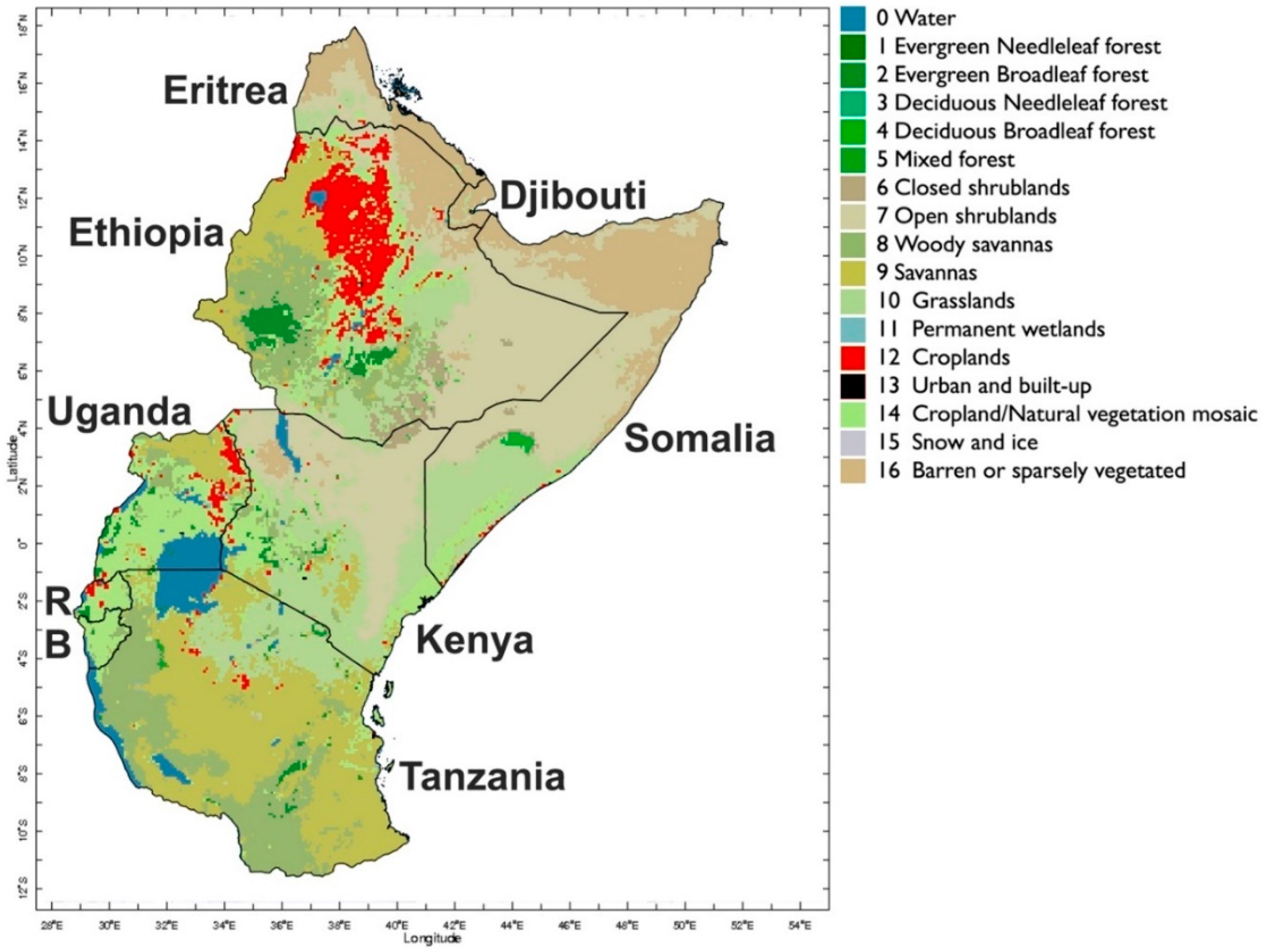
Remotesensing 10 01819 g001
Figure 2. MODIS Moderate Resolution Spectroradiometer (MCD12Q1) Land Cover Dataset (500 m spatial resolution); R = Rwanda, B = Burundi; pixels that classify exclusively as “cropland” are highlighted in red.
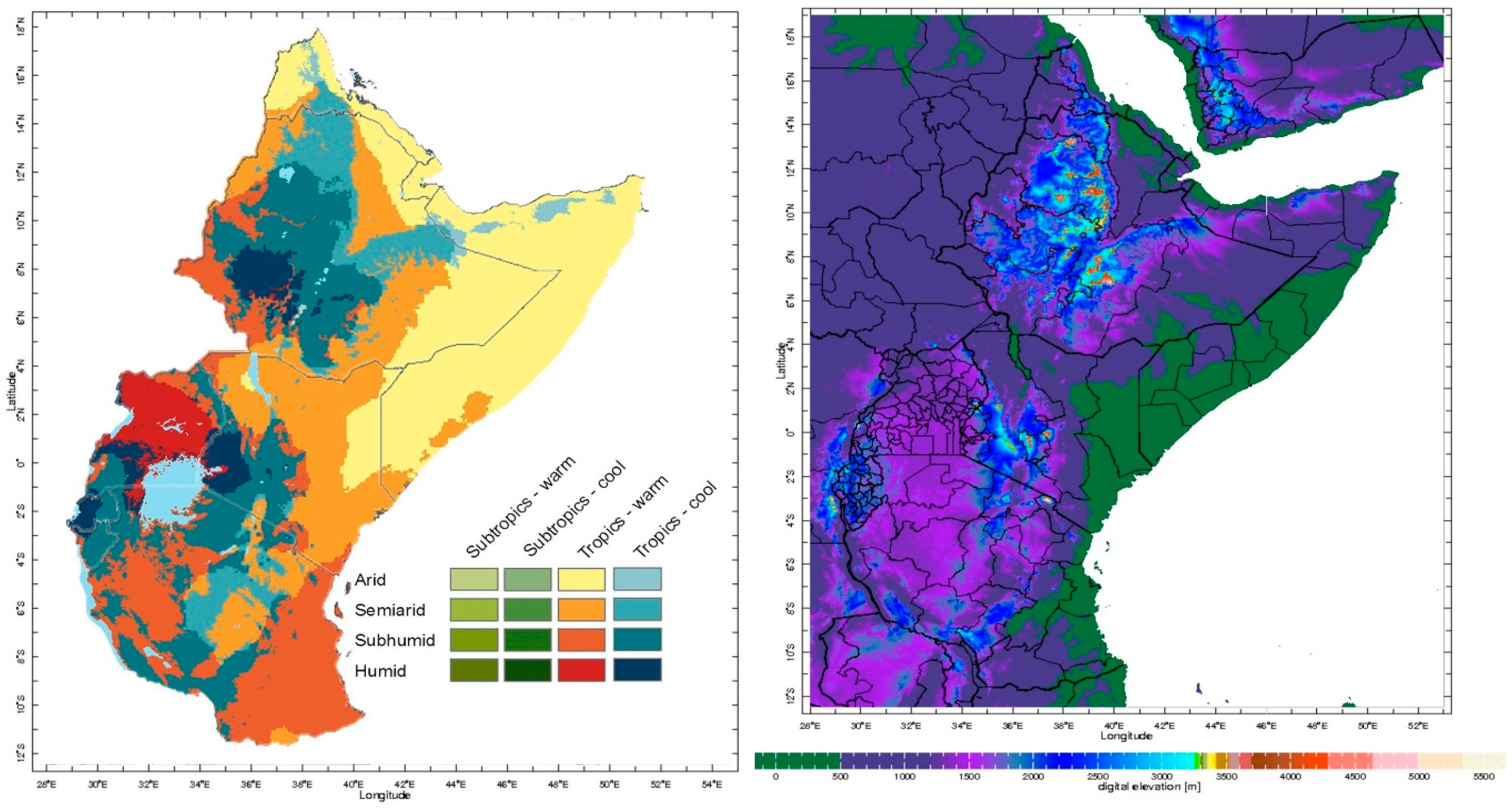
Remotesensing 10 01819 g002
Figure 3. IFPRI agroecological zones (left) and Shuttle Radar Topography Mission (STRM) 90 m topography (right) over the study area.
Remotesensing 10 01819 g003
Figure 4. Annual national maize yield estimates in hectograms (100 grams) per hectare from FAOSTAT for 2000–2016.
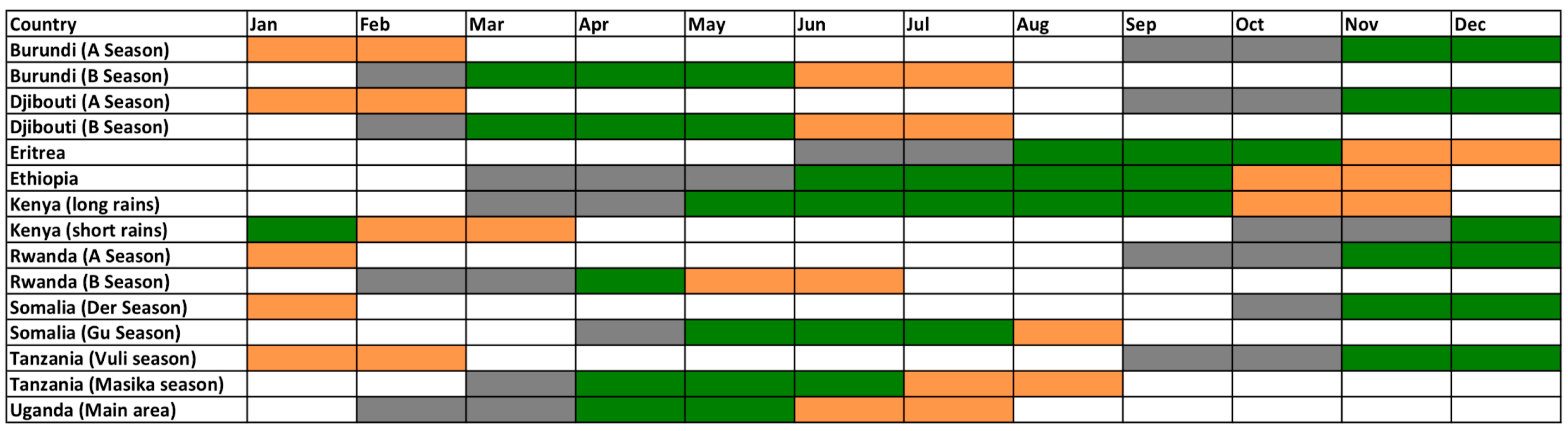
Remotesensing 10 01819 g004
Figure 5. Sowing (grey), growing (green), and harvesting (orange) season in all nine countries (FAO GIEWS).
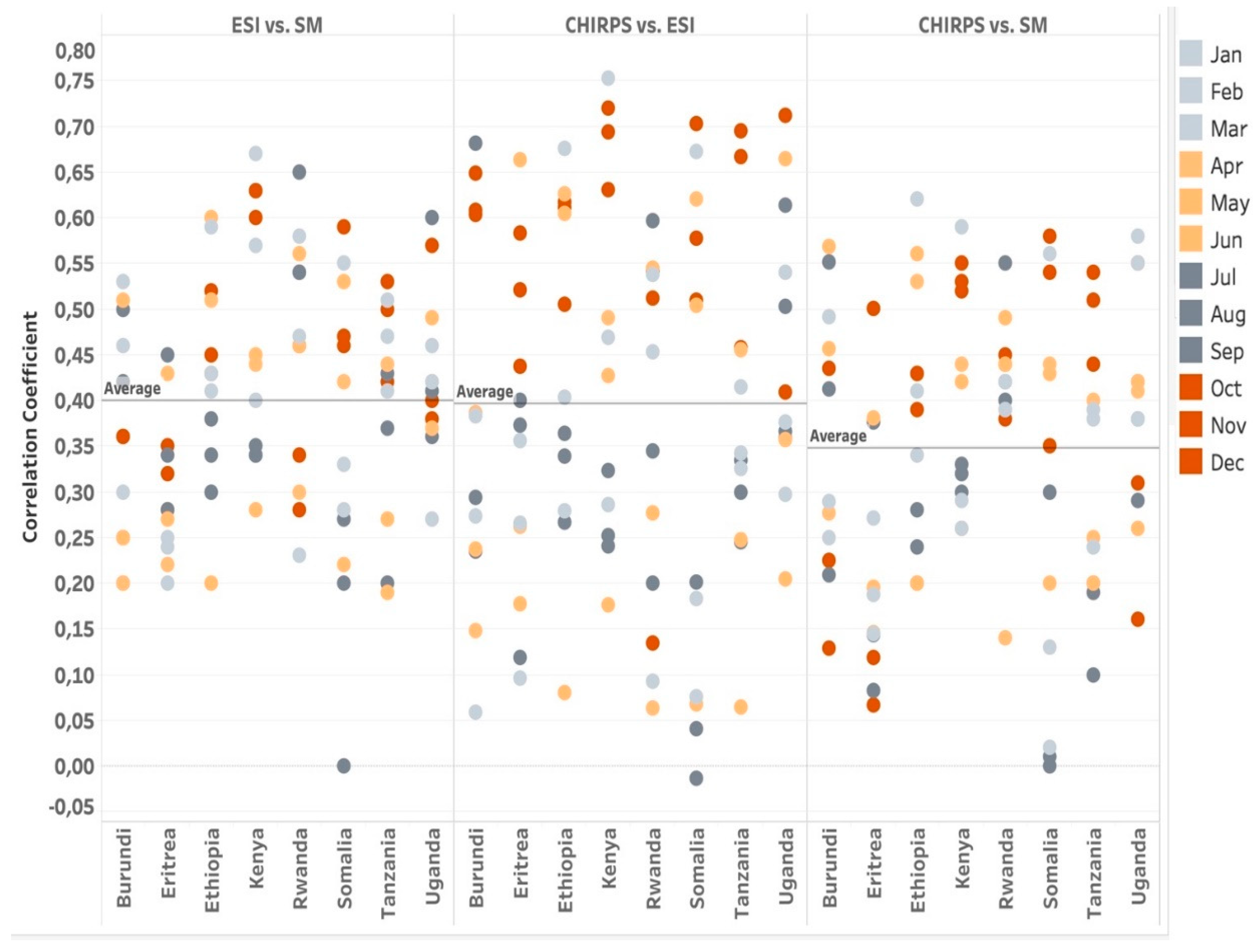
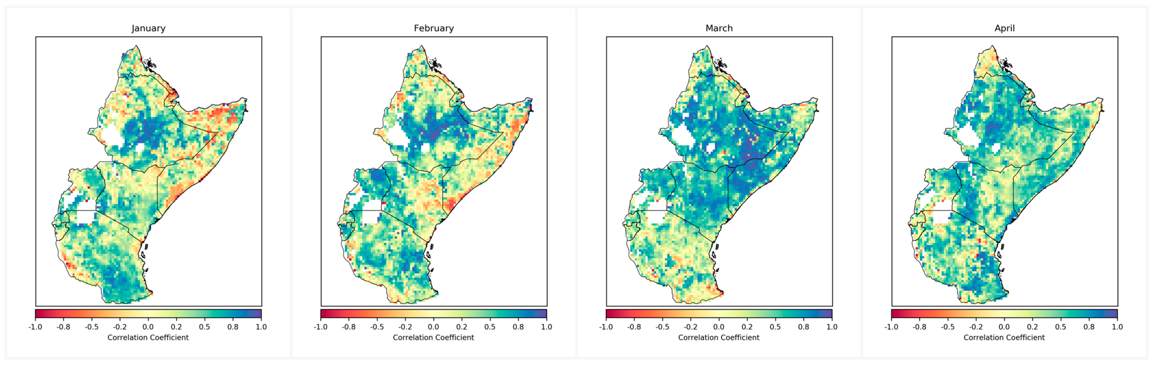
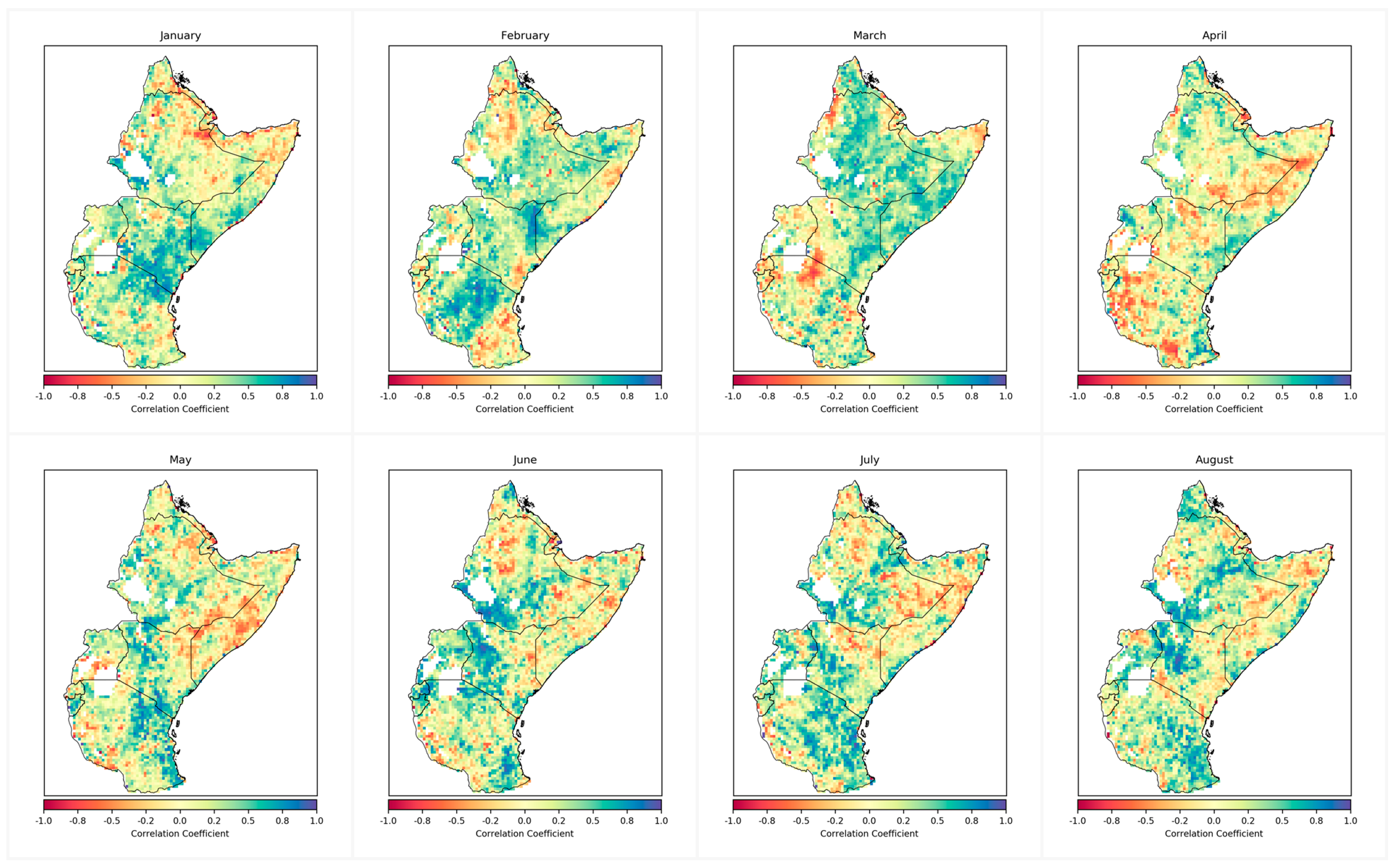
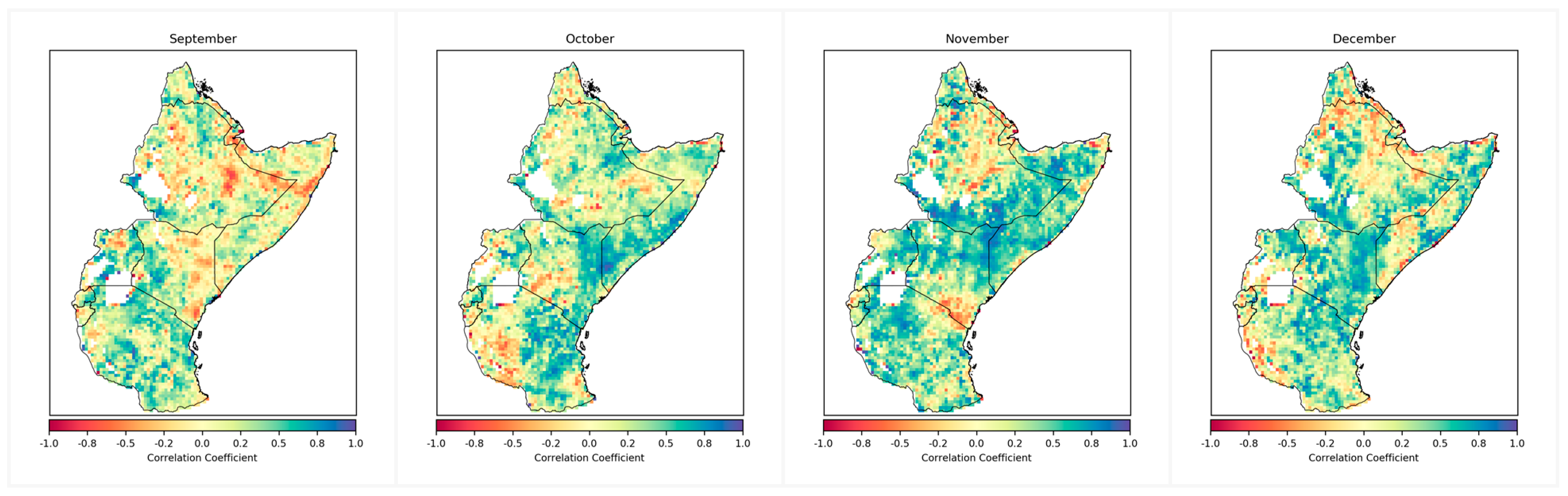
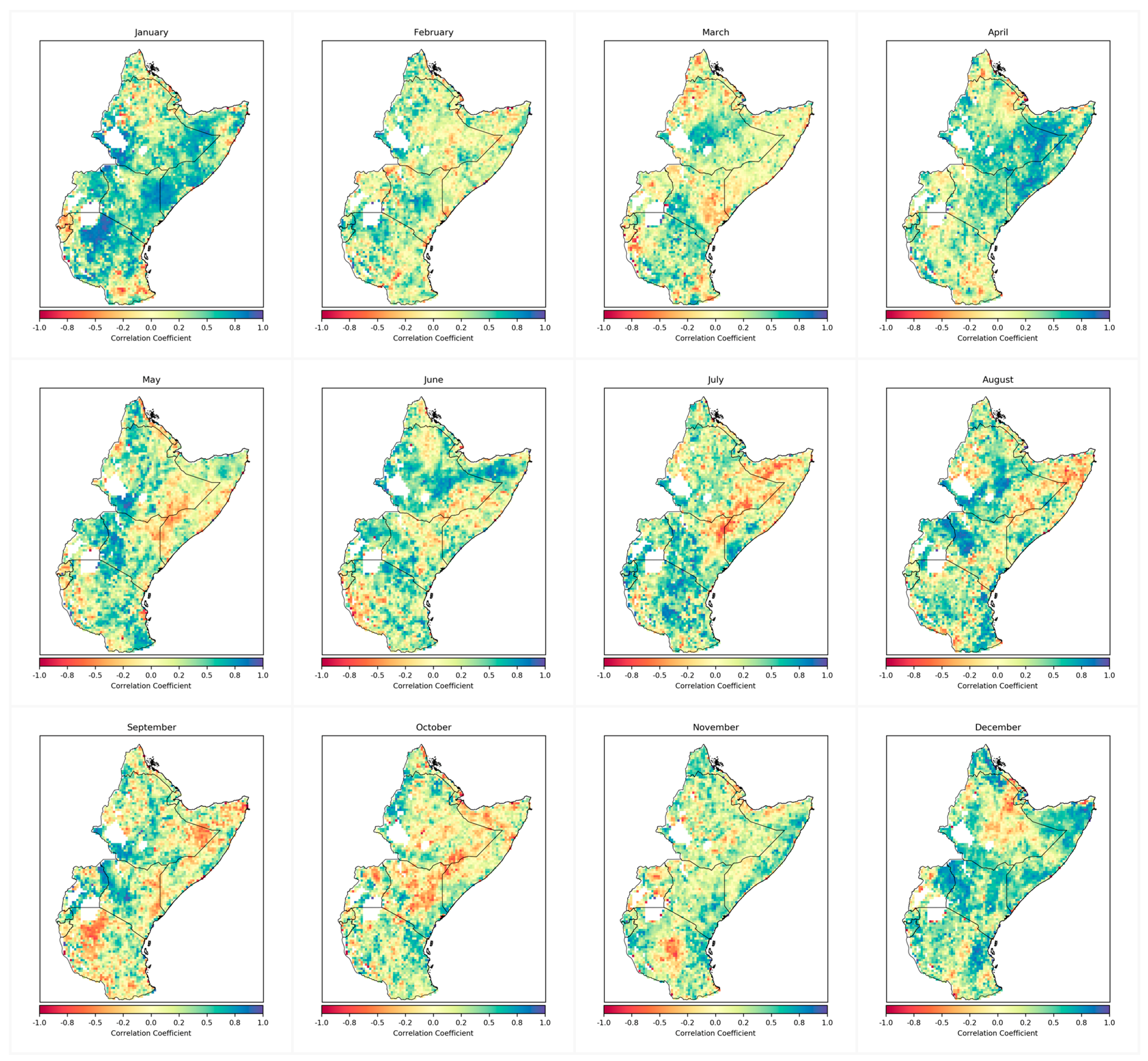
Remotesensing 10 01819 g005
Figure 6. Monthly correlation coefficient between Evaporative Stress Index (ESI) and soil moisture (left), Climate Hazards Group InfraRed Precipitation with Station data (CHIRPS) and ESI (middle), CHIRPS and soil moisture for 2003–2016 for all countries (no mask applied); light-grey and orange represent the first half of the year, dark-grey and orange the second half.
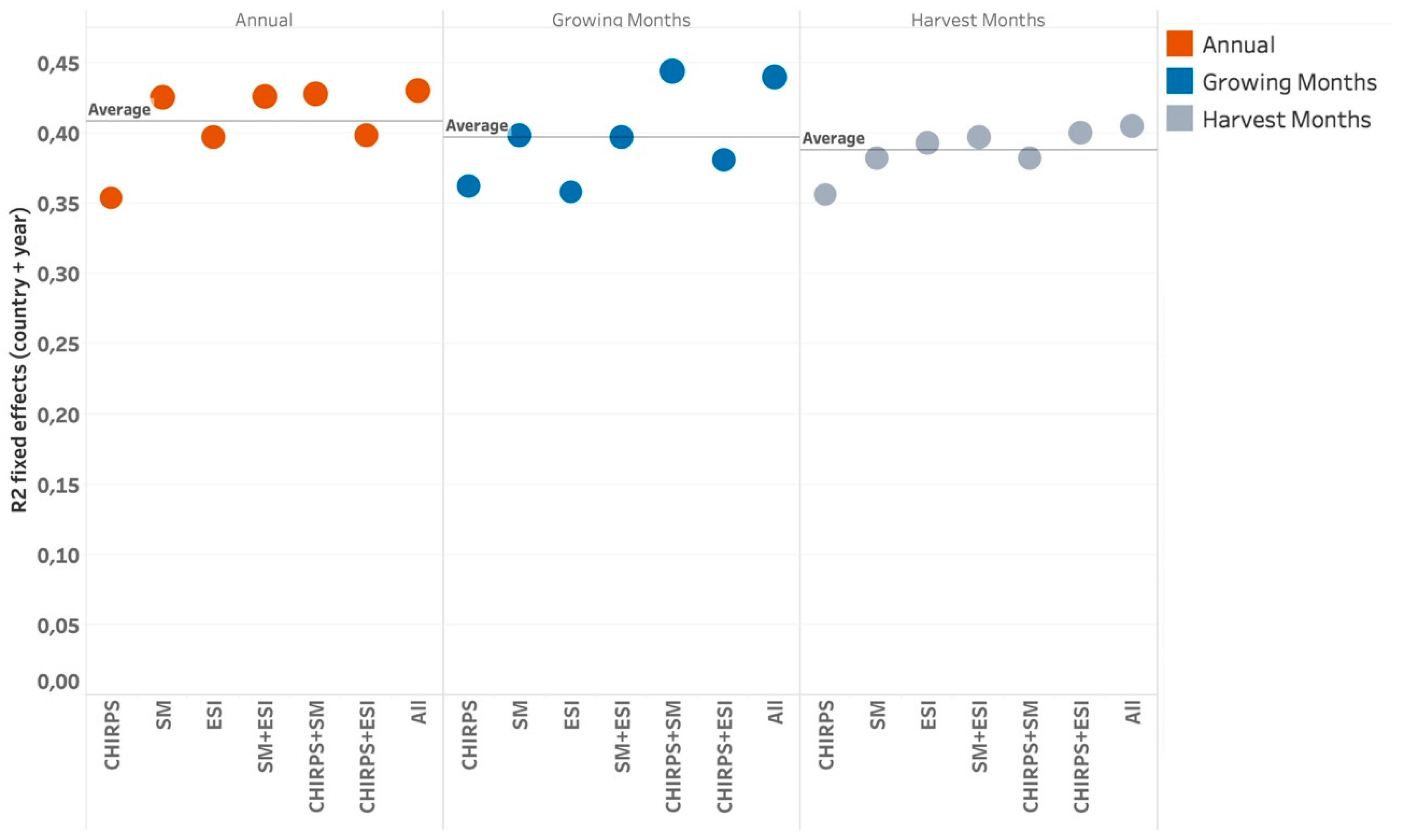
Remotesensing 10 01819 g006
Figure 7. R-squared for all combinations of moisture variables for annual averages of all satellite-derived variables, averages only for maize-growing months (blue) and maize-harvesting months (grey); annual maize yield is the dependent variable.
Remotesensing 10 01819 g007
Table 1. Results of the simple linear regression with fixed effects for standardized anomalies of rainfall (Column 1), soil moisture (Column 2), ESI (Column 3), soil moisture and ESI (Column 4), rainfall and soil moisture (Column 5), rainfall and ESI (Column 6), and all variables combined (Column 7); annual maize yield is the dependent variable: rows represent the regression coefficient for the three independent variables (rainfall, soil moisture, ESI), the regression constant, the number of observations, the R-squared, and the number of countries (8); asterisks mark statistically significant results.
Annual
DEP VARIABLEMaize Yield
(1)(2)(3)(4)(5)(6)(7)
CHIRPS463.50 −996.10−514.20−1054
(1359) (1357)(1375)(1368)
SM 6227 *** 5477 **6688 *** 5842 **
(1867) (2601)(1974) (2650)
ESI 1380 **306.6 1439 **356.4
(540.9)(735.9) (566.1)(740.4)
Constant11,696 ***12,200 ***13,180 ***12,480 ***12,014 ***13,129 ***12,328 ***
(1389)(1290)(1448)(1460)(1318)(1462)(1476)
Observations112112112112112112112
R-squared0.350.430.400.430.430.400.43
Number of Country8888888
Standard errors in parentheses. *** p < 0.01, ** p < 0.05, * p < 0.1.
Table 2. Logit regression results for standardized anomalies of rainfall (Column 1), soil moisture (Column 2), ESI (Column 3), soil moisture and ESI (Column 4), rainfall and soil moisture (Column 5), rainfall and ESI (Column 6) and all variables combined (Column 7); “bad years” are the dependent variable; rows represent the regression coefficient for the three independent variables (rainfall, soil moisture, ESI), the regression constant, the number of observations, the pseudo R-squared, and the number of countries (8); asterisks mark statistically significant results.
Annual
DEP VARIABLEBad Year
(1)(2)(3)(4)(5)(6)(7)
CHIRPS−0.164 −0.125−0.0801−0.0530
(0.232) (0.422)(0.254)(0.477)
SM −0.152 −0.0772−0.0472 −0.0321
(0.232) (0.255)(0.421) (0.479)
ESI −0.897 ***−0.892 *** −0.890 ***−0.890 ***
(0.255)(0.256) (0.256)(0.256)
Constant−1.307 ***−1.306 ***−1.505 ***−1.510 ***−1.307 ***−1.508 ***−1.509 ***
(0.232)(0.232)(0.270)(0.271)(0.232)(0.270)(0.271)
Observations112112112112112112112
Pseudo R20.004330.003680.1220.1220.004440.1220.122
Standard errors in parentheses. *** p < 0.01, ** p < 0.05, * p < 0.1.
Table 3. Results of the simple linear regression with fixed effects focusing on maize-growing months for standardized anomalies of rainfall (Column 1), soil moisture (Column 2), ESI (Column 3), soil moisture and ESI (Column 4), rainfall and soil moisture (Column 5), rainfall and ESI (Column 6), and all variables combined (Column 7); annual maize yield is the dependent variable; rows represent the regression coefficient for the three independent variables (rainfall, soil moisture, ESI), the regression constant, the number of observations, the R-squared, and the number of countries (8); asterisks mark statistically significant results.
Growing Season
DEP VARIABLEMaize Yield
(1)(2)(3)(4)(5)(6)(7)
CHIRPS−1294 −3487 ***−2391 *−3384 **
(1203) (1280)(1324)(1309)
SM 3236 ** 4391 **5000 *** 5588 ***
(1255) (1845)(1375) (1847)
ESI 609.4−585.4 1024 *−324.7
(485.1)(689.6) (531.2)(675.9)
Constant11,535 ***11,804 ***12,109 ***11,740 ***11,778 ***12,198 ***11,766 ***
(1346)(1309)(1478)(1449)(1264)(1460)(1404)
Observations112112111111112111111
R-squared0.360.400.360.400.440.380.44
Number of Country8888888
Standard errors in parentheses. *** p < 0.01, ** p < 0.05, * p < 0.1.
Table 4. Logit regression results focusing on maize-growing months for rainfall (Column 1), soil moisture (Column 2), ESI (Column 3), soil moisture and ESI (Column 4), rainfall and soil moisture (Column 5), rainfall and ESI (Column 6), and all variables combined (Column 7); “bad years” are the dependent variable; rows represent the regression coefficient for the three independent variables (rainfall, soil moisture, ESI), the regression constant, the number of observations, the pseudo R-squared, and the number of countries (8); asterisks mark statistically significant results.
Growing Season
DEP VARIABLEBad Year
(1)(2)(3)(4)(5)(6)(7)
CHIRPS−0.0271 0.3330.05230.330
(0.231) (0.397)(0.247)(0.415)
SM −0.174 −0.0810−0.446 −0.348
(0.233) (0.248)(0.402) (0.419)
ESI −0.570 **−0.559 ** −0.576 **−0.561 **
(0.241)(0.243) (0.242)(0.243)
Constant1.299 ***1.308 ***1.429 ***1.432 ***1.319 ***1.429 ***1.443 ***
(0.230)(0.232)(0.251)(0.251)(0.234)(0.251)(0.254)
Observations112112111111112111111
Pseudo R20.0001180.004840.05220.05310.01090.05260.0587
Standard errors in parentheses. *** p < 0.01, ** p < 0.05, * p < 0.1.
Table 5. Results of the simple linear regression with fixed effects focusing on maize-harvesting months for standardized anomalies of rainfall (Column 1), soil moisture (Column 2), ESI (Column 3), soil moisture and ESI (Column 4), rainfall and soil moisture (Column 5), rainfall and ESI (Column 6) and all variables combined (Column 7); annual maize yield is the dependent variable; rows represent the regression coefficient for the three independent variables (rainfall, soil moisture, ESI), the regression constant, the number of observations, the R-squared, and the number of countries (8); asterisks mark statistically significant results.
Harvesting Season
DEP VARIABLEMaize Yield
(1)(2)(3)(4)(5)(6)(7)
CHIRPS545.50 −124.50−1009−1108
(914.4) (964.3)(980.0)(989.1)
SM 2611 ** 11102675 * 1326
(1278) (1585)(1376) (1595)
ESI 1104 ***889.4 * 1310 ***1074 **
(385.4)(493.3) (434.2)(519.4)
Constant11,697 ***11,826 ***13,722 ***13,715 ***11,807 ***13,728 ***13,721 ***
(1363)(1328)(1513)(1518)(1344)(1513)(1515)
Observations112112110110112110110
R-squared0.360.380.390.400.380.400.41
Number of Country8888888
Standard errors in parentheses. *** p < 0.01, ** p < 0.05, * p < 0.1.
Table 6. Logit regression results focusing on maize-harvesting months for rainfall (Column 1), soil moisture (Column 2), ESI (Column 3), soil moisture and ESI (Column 4), rainfall and soil moisture (Column 5), rainfall and ESI (Column 6) and all variables combined (Column 7); “bad years” are the dependent variable; rows represent the regression coefficient for the three independent variables (rainfall, soil moisture, ESI), the regression constant, the number of observations, the pseudo R-squared and the number of countries (8); asterisks mark statistically significant results.
Harvest Season
DEP VARIABLEBad Year
(1)(2)(3)(4)(5)(6)(7)
CHIRPS−0.108 −0.001450.3340.448
(0.231) (0.330)(0.317)(0.411)
SM −0.149 0.117−0.148 −0.166
(0.231) (0.280)(0.336) (0.392)
ESI −1.022 ***−1.063 *** −1.153 ***−1.142 ***
(0.296)(0.315) (0.333)(0.334)
Constant−1.303 ***−1.306 ***−1.662 ***−1.672 ***−1.306 ***−1.715 ***−1.720 ***
(0.231)(0.232)(0.295)(0.297)(0.232)(0.307)(0.308)
Observations112112110110112110110
Pseudo R20.001900.003590.1320.1340.003590.1430.144
Standard errors in parentheses. *** p < 0.01, ** p < 0.05, * p < 0.1.

