Opium Poppy Detection Using Deep Learning


1
Institute of Remote Sensing and Digital Earth, Chinese Academy of Sciences, Beijing 100101, China
2
University of Chinese Academy of Sciences, Beijing 100049, China
*
Authors to whom correspondence should be addressed.
Remote Sens. 2018, 10(12), 1886; https://doi.org/10.3390/rs10121886
Submission received: 16 October 2018
/
Revised: 16 November 2018
/
Accepted: 20 November 2018
/
Published: 27 November 2018
Abstract
:Opium poppies are a major source of traditional drugs, which are not only harmful to physical and mental health, but also threaten the economy and society. Monitoring poppy cultivation in key regions through remote sensing is therefore a crucial task; the location coordinates of poppy parcels represent particularly important information for their eradication by local governments. We propose a new methodology based on deep learning target detection to identify the location of poppy parcels and map their spatial distribution. We first make six training datasets with different band combinations and slide window sizes using two ZiYuan3 (ZY3) remote sensing images and separately train the single shot multibox detector (SSD) model. Then, we choose the best model and test its performance using 225 km2 verification images from Lao People’s Democratic Republic (Lao PDR), which exhibits a precision of 95% for a recall of 85%. The speed of our method is 4.5 km2/s on 1080TI Graphics Processing Unit (GPU). This study is the first attempt to monitor opium poppies with the deep learning method and achieve a high recognition rate. Our method does not require manual feature extraction and provides an alternative way to rapidly obtain the exact location coordinates of opium poppy cultivation patches.
1. Introduction
Drugs cause many problems worldwide. They are not only harmful to human health, they also lead to family breakdown. Each year, almost hundreds of thousands of people die prematurely because of drug abuse. According to the World Health Organization (WHO), approximately 450,000 people died as a result of drug use in 2015. The countries with the most potential for opium poppy cultivation are Afghanistan, Myanmar, Mexico, and Lao PDR. In order to effectively understand the global poppy cultivation situation, the United Nations Office on Drugs and Crime (UNODC) has been monitoring these key regions and publishing annual planting reports since the early 1990s. Until the early 2000s, they used socioeconomic data as the basis for their annual Afghanistan poppy survey. However, this not only involves a lot of manpower and material resources, the field work is also extremely difficult due to poor traffic conditions in poppy-growing areas and problems ensuring human safety.
Satellite remote sensing technology can take photos of any area on the Earth’s surface, and has developed rapidly in recent decades; it is now used to map many types of land cover [1,2]. Thus, remote sensing is becoming an effective weapon in the war on drugs. In the 1990s, Chuinsiri et al. estimated the opium poppy cultivation situation in the Chiang Mai province of Thailand using Landsat TM data [3], and found that the local climate, geographical conditions, and planting calendar are all important for identifying opium poppies. Since 2002, the UNODC has been monitoring poppy cultivation in Afghanistan by interpreting high-resolution (≤1 m) satellite images. In 2005, they randomly selected 79 location points from major agricultural areas in the 15 provinces of Afghanistan, then covered each location point with two phases (before and after poppy harvest) of IKONOS images (10 km × 10 km). Additionally, up to four areas measuring 250 m × 250 m were selected randomly from each IKONOS image and field measured by trained Afghan surveyors to determine the regions corresponding to poppy parcels and other crops. The ground data was used to identify land-cover types in the image areas for training the subsequent digital classifier and assessing its accuracy. With this method of sampling, they estimated the extent of poppy cultivation in Afghanistan [4]. However, the sampling method cannot obtain the spatial distribution and coordinates of opium poppy parcels [5], which is key information that is required by the local authority in order to eradicate opium poppies before harvest. Thus, the Chinese National Narcotics Control Commission (CNNCC) began monitoring poppy cultivation using remote sensing images and publishing annual reports for north Myanmar since 2006 and north Lao PDR since 2012. The CNNCC covers all of the monitoring regions with multi-period high-resolution satellite images and determines poppy fields in the monitoring area using a machine learning method combined with field measurements.
Some studies have proposed different methods to improve the poppy detection accuracy or efficiency of remote sensing image-based techniques. Simms et al. used imagery-based stratification [6] and image segmentation [7] to improve opium cultivation estimates in Afghanistan, but estimates were still based on sampling methods. Jia et al. [8] demonstrated that opium poppies could be distinguished from coexisting crops in many surveyed wavebands using a field survey spectrum at the canopy level on an official poppy-growing region in China. Using hyperspectral imagery, Wang et al. [9] identified poppy parcels in Afghanistan and found a significant difference between poppy and wheat using unsupervised endmember selection and multiple endmember spectral mixture analysis on EO-1 Hyperion imagery. Then, they generated a poppy distribution map with an overall accuracy of 73%. In 2016, the same group used an unsupervised mixture-tuned matched filtering (MTMF)-based method to detect poppies, which was more than 10 times faster than their previous method that had similar detection accuracy [10]. This research provided a way to rapidly monitor poppy cultivation over large areas; however, the detection accuracy is relatively low.
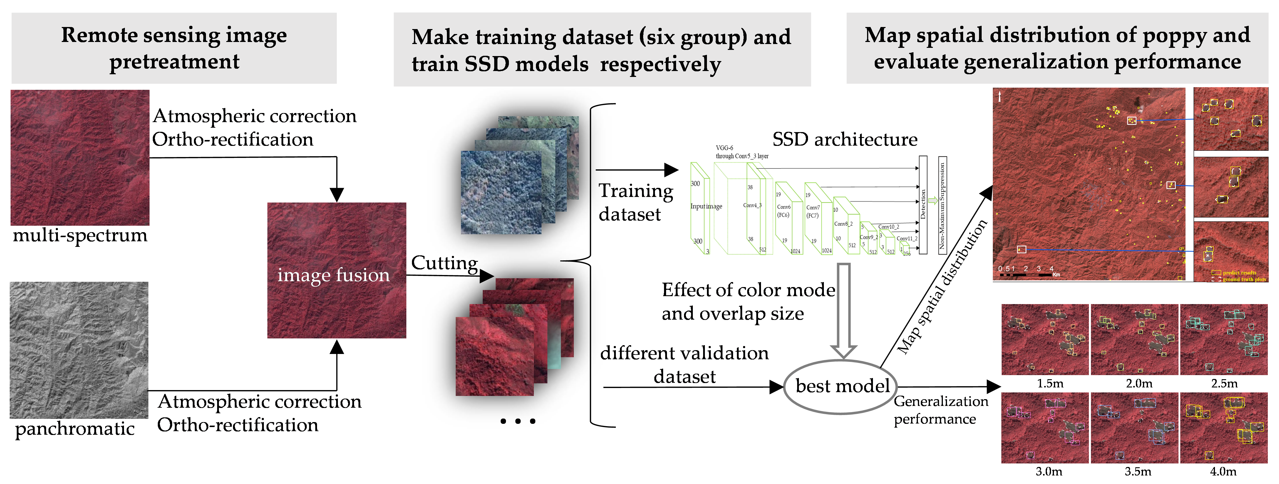
Until now, most studies have been conducted in Afghanistan, and only a few have been conducted in Lao PDR; however, both the environment and characteristics of poppy planting differ between the two countries. We know that the annual production of opium poppies in Afghanistan exceeds 85% of the global production. In Afghanistan, the poppy is grown predominantly within irrigated areas along river valleys together with other crops, and poppy fields are no different in size to fields containing other crops [11]. However, in Lao PDR, most of the opium poppies are planted on steep slopes, where a small patch of forest is logged and burnt before planting; most poppy parcels are far from residential and main roads, and the shape and size of poppy parcels differ from that of agricultural parcels (Figure 1).
The Lao PDR government organizes personnel to eradicate opium poppies each year, so it is important to obtain location information for every poppy field. In order to obtain the coordinates of opium poppy parcels, we attempt to identify them using the object detection method. Object detection with remote sensing images has experienced the following development process: (1) template matching-based object detection [12,13], (2) knowledge-based object detection [14,15], (3) object-based image analysis (OBIA) object detection [16,17], (4) machine learning-based object detection [18,19,20], and (5) deep learning-based object detection.
Deep learning-based object detection was proposed after development of the deep convolutional neural network (DCNN) [21]. DCNNs comprise multiple convolutional layers and are capable of learning high-level abstract features from the original pixel values of images; they have recently demonstrated impressive levels of performance in image classification tasks [22,23,24] and image processing [25]. One of the most prominent advantages of deep learning methods is that feature extraction does not require manual intervention, but rather is automatically extracted from a large amount of training data [26]. For object detection tasks, a series of neural network models have been proposed, including region-based convolutional neural networks (RCNN), faster variants [27,28,29], and end-to-end convolutional neural networks [30,31]. RCNN series network training is divided into several stages, which are time-consuming and slow in the model prediction stage. A single shot multibox detector (SSD) is the state-of-art method for object detection. It integrates the entire detection process in a single deep neural network, ensuring efficient object detection, especially in multi-scale detection [31]. SSD only requires an input image and ground truth boxes of the target during training. At the front of the network, Visual Geometry Group (VGG)-16 is used, not including classification layers, as the base network to extract low and middle-level visual features. Then, convolutional feature layers are added after the VGG-16 network, which progressively decrease in size and allow predictions of detections at multiple scales; they produce a fixed-size collection of bounding boxes and scores for the presence of objects. At the end of the network, non-maximum suppression is employed to choose the best prediction boxes with higher confidence. Ye et al. [32] utilized SSD to detect wharves within coastal zones using remote sensing images, achieving an accuracy of 90.9% and a recall rate of 74.5%. Researchers at Missouri State University [33] used deep learning algorithms to identify Chinese surface-to-air missiles and improve the efficiency of data analysts by a factor of 81. Wang et al. [34] detected ships from synthetic aperture radar (SAR) images using SSD with a probability of detection of 0.978. Zhang et al. [35] achieved good results utilizing remote sensing images to detect aircraft.
These studies prove that deep learning-based object detection can exhibit good recognition effects on remote sensing images. Therefore, this study attempts to detect opium poppy cultivation areas in Lao PDR using the deep learning-based object detection method. Specifically, we detect the location of every poppy parcel on remote sensing images using the SSD network, and explore the prediction performance of different parameters.
2. Materials and Methodology
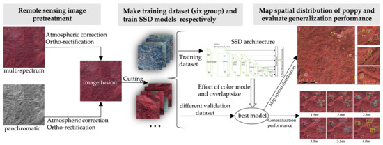
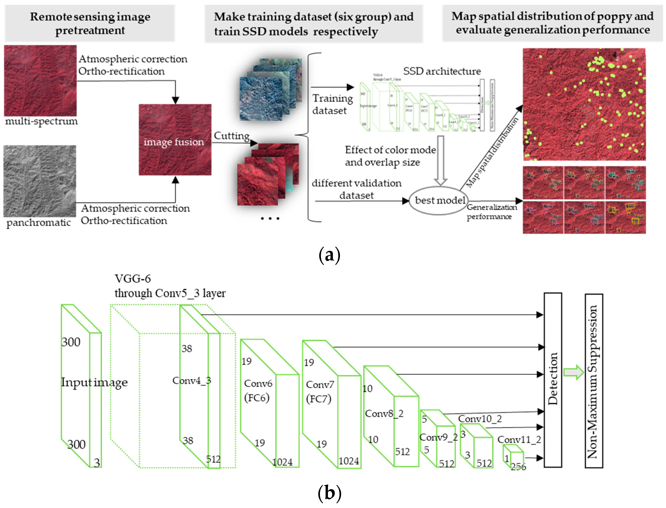
We constructed a detailed workflow for detecting opium poppy parcels and analyzing the results (Figure 2a), as well as an architecture for an SSD model (Figure 2b). This workflow included two major components. First, we pretreated the remote sensing images (see Section 2.2.1); after that, we made six group datasets based on different color modes (near infrared–red–green (NRG) and red–green–blue (RGB)), and different overlap sizes (100, 150, 200), and then used them to train the SSD model, respectively. Then, we explored the effect of different datasets on recognition accuracy, and obtained the best model. Next, we utilized the best model to map the spatial distribution of poppy parcels, and conducted a series of comparison experiments on different spatial resolution verification images and on another type of satellite image to demonstrate the generalization performance of our model.
2.1. Study Area
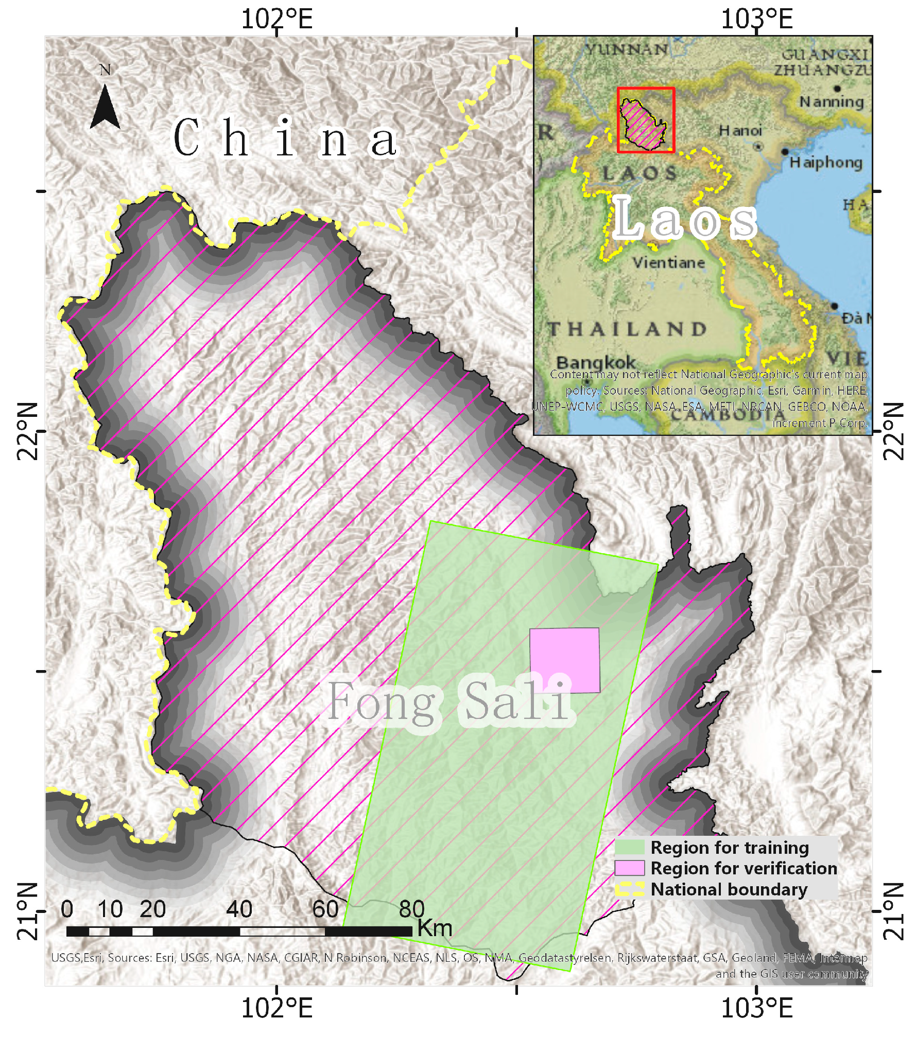
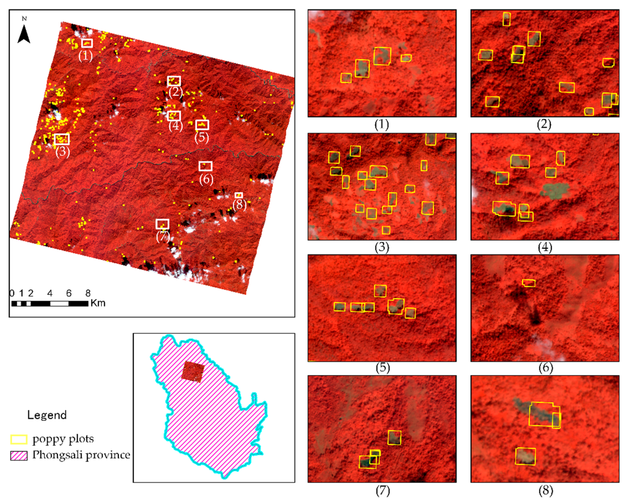
Lao PDR is a corner of the Golden Triangle, which is one of the world’s main sources of drugs. According to “Opium Poppy Monitoring in Laos” (CNNCC), Phongsali is the dominant opium cultivating province in Lao PDR. In the 2016–2017 growing season, approximately 2917 hectares of opium poppies were found in Phongsali province, accounting for 54.76% of the total cultivation of Lao PDR [36]. Phongsali province is in the northernmost part of Lao PDR, bordering China’s Yunnan province in the west and north, and Vietnam in the east. Our study area is part of Phongsali province, covering an area of 4800 km2 (Figure 3).
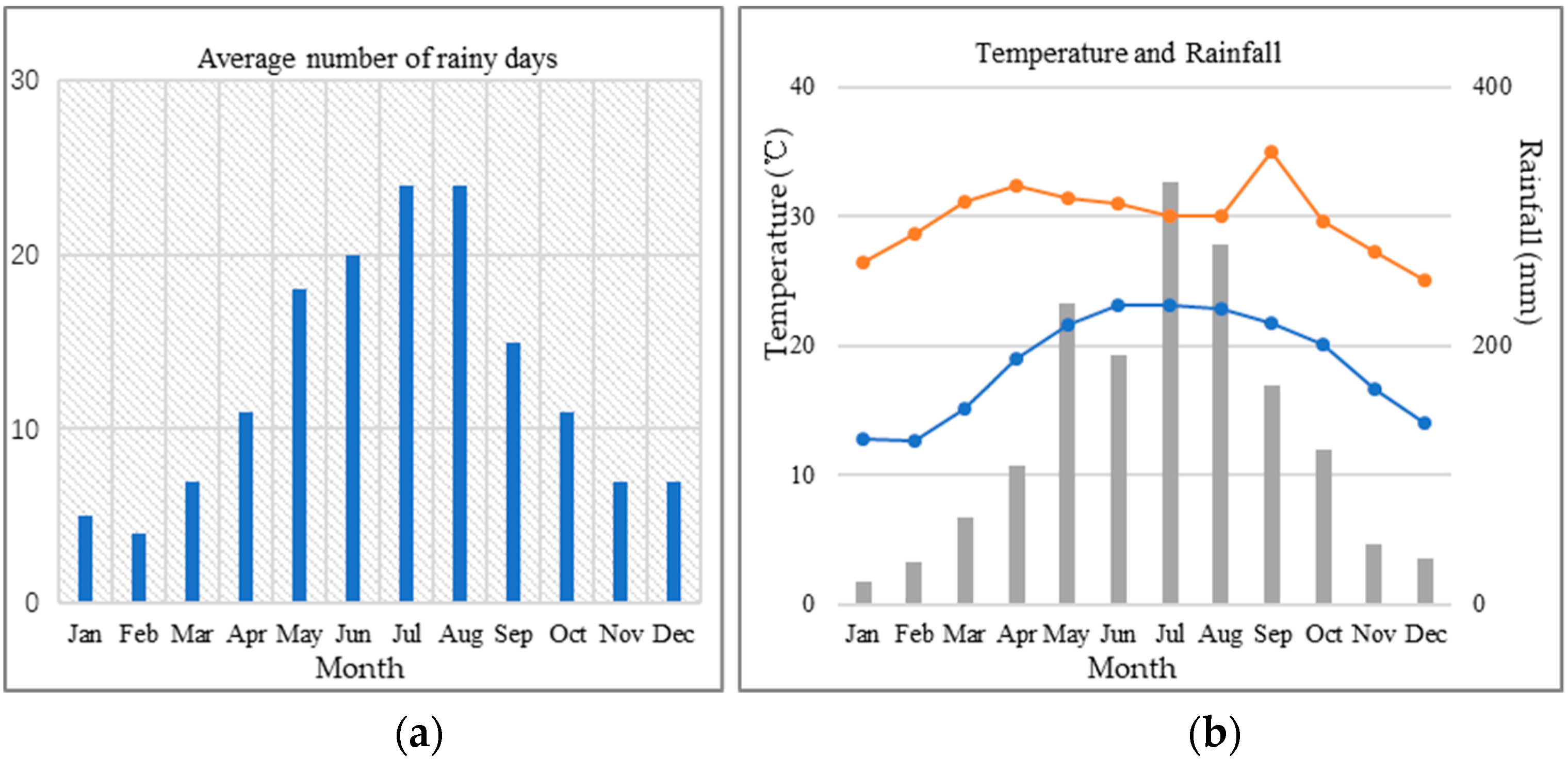
Phongsali province is predominantly mountainous with elevation ranging from 356 m to 1907 m above sea level. It receives a large amount of rain; annual precipitation ranges from 1700 mm to 2060 mm, but there is a clear distinction between the rainy season (May–October) and the dry season (November–April) (Figure 4a). The annual average temperatures reach a maximum of 35 °C during September and a minimum of 14 °C during December and January (Figure 4b). Diverse forest types consisting of tropical rainforest, monsoon forest, and low mountainous forest cover more than 80% of the region [37]. This combination of light, water, and heat is ideal for poppy cultivation. Some studies [38] have suggested that the end of the rainy season (November–December) is the best time to extract opium poppies in the Golden Triangle. A calendar of opium poppy planting is important for monitoring with remote sensing data. Due to the unique climate in Phongsali, the logging–drying–ploughing–seeding process begins from the end of September. The details of the planting calendar are shown in Table 1.
2.2. Data Collection
2.2.1. Remote Sensing Images
The ZiYuan3 (ZY3) satellite of China was launched on 9 January 2012. Its spatial resolution is 2.1 m in panchromatic and 5.8 m in multi-spectrum, and each image can cover a region measuring 2500 km2. According to the cultivation calendar of poppies in Phongsali province, we selected two ZY3 images acquired on 22 November 2016 to train and test our SSD model. We also chose GaoFen-2 (GF-2) to test the generalization performance of our method. GF-2 was launched on 19 August 2014, and its spatial resolution is 0.8 m in panchromatic and 3.2 m in multi-spectrum. Each GF-2 image can cover a region measuring 480 km2. We selected one GF-2 multi-spectrum (3.2 m) image to evaluate our method performance. These remote sensing images were all obtained from the China Centre for Resources Satellite Data and Application (CRESDA) (http://www.cresda.com/CN/index.shtml), and their detailed parameters are shown in Table 2.
A series of data pre-processing steps was conducted using modules of the Environment for Visualizing Images software (ENVI, Version 5.3, Environmental Systems Research Institute, Inc., HRS-Harris Corporation, FL, USA) and ArcGIS (Version 10.5, Environmental Systems Research Institute, Inc., Esri, CA, USA), including radiometric calibration using parameters provided by CRESDA, atmospheric correction using the Fast Line-of-sight Atmospheric Analysis of Spectral Hypercube (FLAASH), and orthorectification using the Rational Polynomial Coefficients (RPC) orthorectification module based on Google Earth and Digital Elevation Model (DEM, SRTM 90 m). In order to retain both spectral information in the multi-spectrum image and high spatial resolution in the panchromatic images, we also performed image fusion using Nearest Neighbor Diffusion (NNDiffuse) pan sharpening on ZY3 images, and resized its resolution from 2.1 m to 2.0 m.
2.2.2. Ground Truth Data
The poppy fields in our study area were provided by the CNNCC. Since 2012, monitoring and field survey work in northern Lao PDR has been conducted annually by the CNNCC and the Lao National Commission for Drug Control and Supervision (LCDC). As part of “Opium Poppy Monitoring in Laos 2016”, the final opium poppy map was verified by both China and Lao PDR surveyors. We used part of this final poppy map as surrogate ground truth data.
2.3. Methodology
2.3.1. Training Datasets
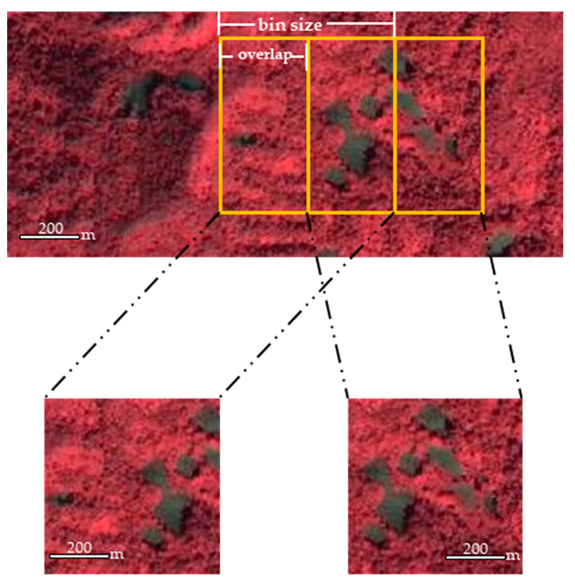
The pixel size of the input picture for the SSD model must be 300 pixels × 300 pixels with three bands, whereas a ZY3 image has approximately 30,000 pixels × 30,000 pixels with four bands. Thus, we had to partition the entire remote sensing image into multiple small patch pictures. Partitioning was performed via a sliding window with user-defined bin sizes and overlap, as shown in Figure 5. The bin size was fixed to 300 pixels, and the overlap was set between one and 300. We only retained three bands of the remote sensing image, and explored which combination of the three bands produced the optimal model.
The ground truth data of poppy parcels were vector polygons surrounding the target. We had to transform the polygon file into the external rectangle pixel coordinates required by the model. Based on the ground truth data, we made a label for each patch (if no target existed on the patch, the sample was discarded). This contained at least one poppy target for each sample picture in the training datasets, and each sample picture had a corresponding annotation file that contained the bounding box’s coordinates.
In our experiment, in order to explore the effect of color mode and overlap size, we made six group datasets, and for each dataset, we calculated the total number of picture samples and poppy parcels targets (Table 3). In the end, 80% of each dataset was used for training, and 20% was used for testing.
2.3.2. Training Strategy
The entire SSD network contained 2,337,782 parameters to train, which required a large number of labeled pictures. However, this portion of our datasets was still too small to train the network from initialization. Nevertheless, Hu et al. [39] provided a feasible solution, whereby the rich low and middle-level features learned from convolutional neural networks are transferable to a variety of visual recognition tasks. It is generally accepted that remote sensing images and natural images are similar in low-level and middle-level features, so we used the parameters of the first few layers of the neural network trained on tens of millions of natural images as the parameters of our network. In this way, we only needed to use our samples to train the parameters in the latter part of the network to extract the high-level semantic information of the image.
For the data augmentation of each sample image, we performed the following operations to generate new samples:
- random changes in saturation, brightness, and contrast ratio;
- flip horizontally and vertically;
- cut to random size.
These operations increased the size of the training sample by a factor of approximately 30, which helps improve the generalization performance of the model.
The model contained many hyperparameters; therefore, many experiments were performed to determine the final parameters shown in Table 4.
2.3.3. Post-Processing
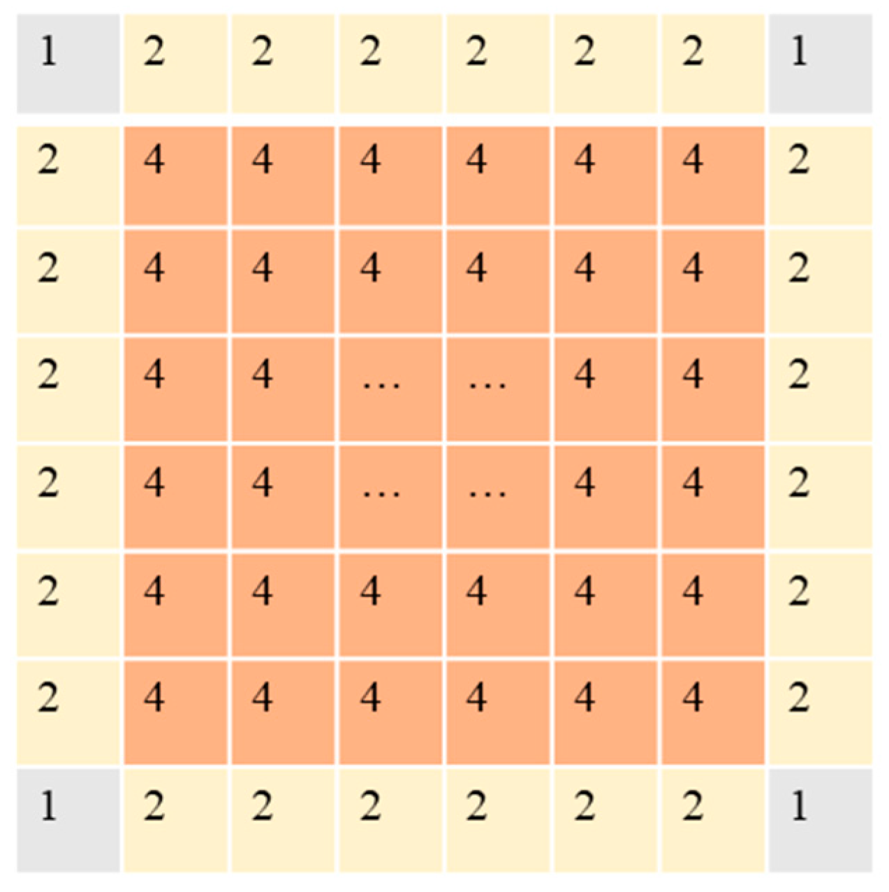
The SSD model prediction results provide a confidence index (Conf) for every poppy plot of the image. Typically, we used results above a certain threshold (0.4) as the final prediction result. In order to evaluate the identification effect of poppy parcels effectively and reasonably, the input whole image was processed with a sliding window in the prediction stage, and the overlap was set to 150 pixels. Then, according to the polygon geographic coordinates in each patch (300 pixels × 300 pixels), we merged them into a whole vector file called Ori-results. In this way, we could make four predictions for most of the parts of the whole image: two predictions for the edge parts, and one prediction for the four corners, as shown in Figure 6.
We propose that the more times (Num) a location was predicted as the target parcel, the higher its confidence. Of course, we consider the initial Conf, so we proposed a new confidence index to indicate the poppy confidence. First, we modified the Conf with Num as shown in Equation (1), and then normalized the W_Conf to 0.4–1.0 as shown in Equation (2), where W_Confmax and W_Confmin are the maximum and minimum values of W_Conf, respectively, and Confnew is the final confidence of every poppy parcel.
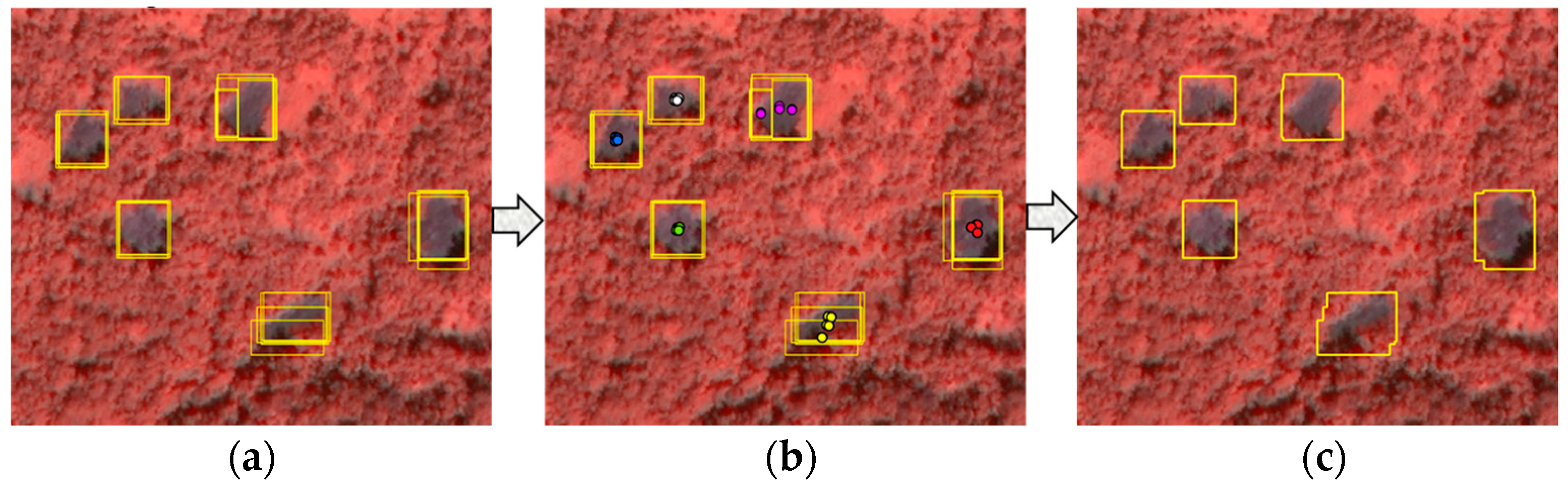
For all the Ori-results polygons (Figure 7a), we first obtained their center coordinate points, and then conducted Density-Based Spatial Clustering of Applications with Noise (DBSCAN) [40] for these points (Figure 7b). We then calculated the mean Conf of the Ori-results polygon and its count (Num) based on the same clustering. Finally, we merged the Ori-results polygons into one union polygon and preserved their properties (mean Conf and Num) (Figure 7c), eventually calculating the final confidence values using Equations (1) and (2). All of the post-processing steps were conducted using ArcGIS10.5 software.
2.3.4. Accuracy Assessment
We used a precision–recall curve and the F1 score to evaluate the model performance at recognizing poppy parcels. Precision, recall, and F1 score are defined as follows:
where TP represents true positives, FN represents false negatives, and FP represents false positives. The F1 score is a good evaluation index that considers both precision and recall. For different confidence thresholds, the precision and recall rate will be different. We increased the confidence threshold value of the final results from 0.4 to 1 at an interval of 0.01, and calculated the corresponding precision and recall values, then plotted the precision–recall curve and F1 curve.
3. Experiments and Results
3.1. Effect of Different Sliding Window Size
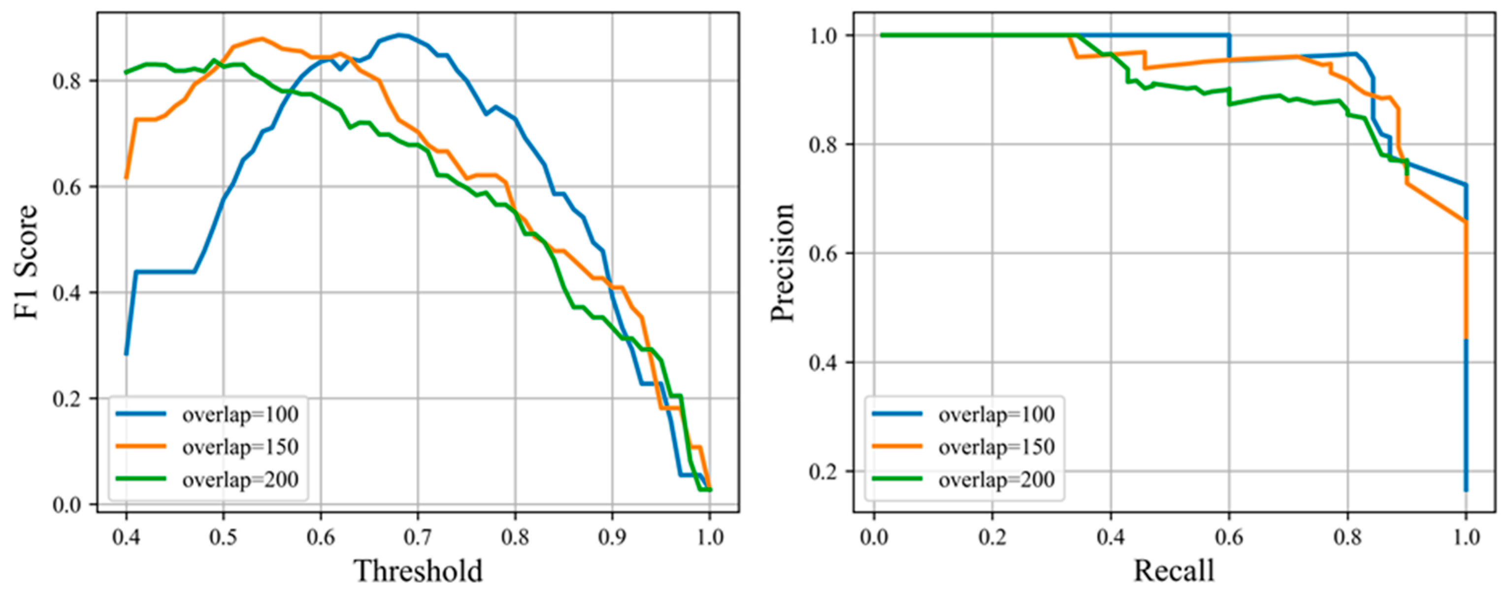
We used the sliding window method to generate the training samples, yet the different overlap values have different effects on the results. First, we generated different training datasets by setting the overlap to 100, 150, and 200 and trained three different models accordingly, comparing their prediction performance on the verification image.
The F1 score and precision–recall curve are shown in Figure 8. When the overlap is set to 100, the maximum F1 score is 0.885, and the precision–recall curve tends toward the upper right. When the overlap is set to 150, the maximum F1 score is 0.879 and the precision–recall curve is better than with an overlap of 200, but worse than with an overlap of 100. When the overlap is set to 200, the maximum F1 score is 0.838, and the precision–recall curve is below the other two curves.
3.2. Effect of Band Combinations
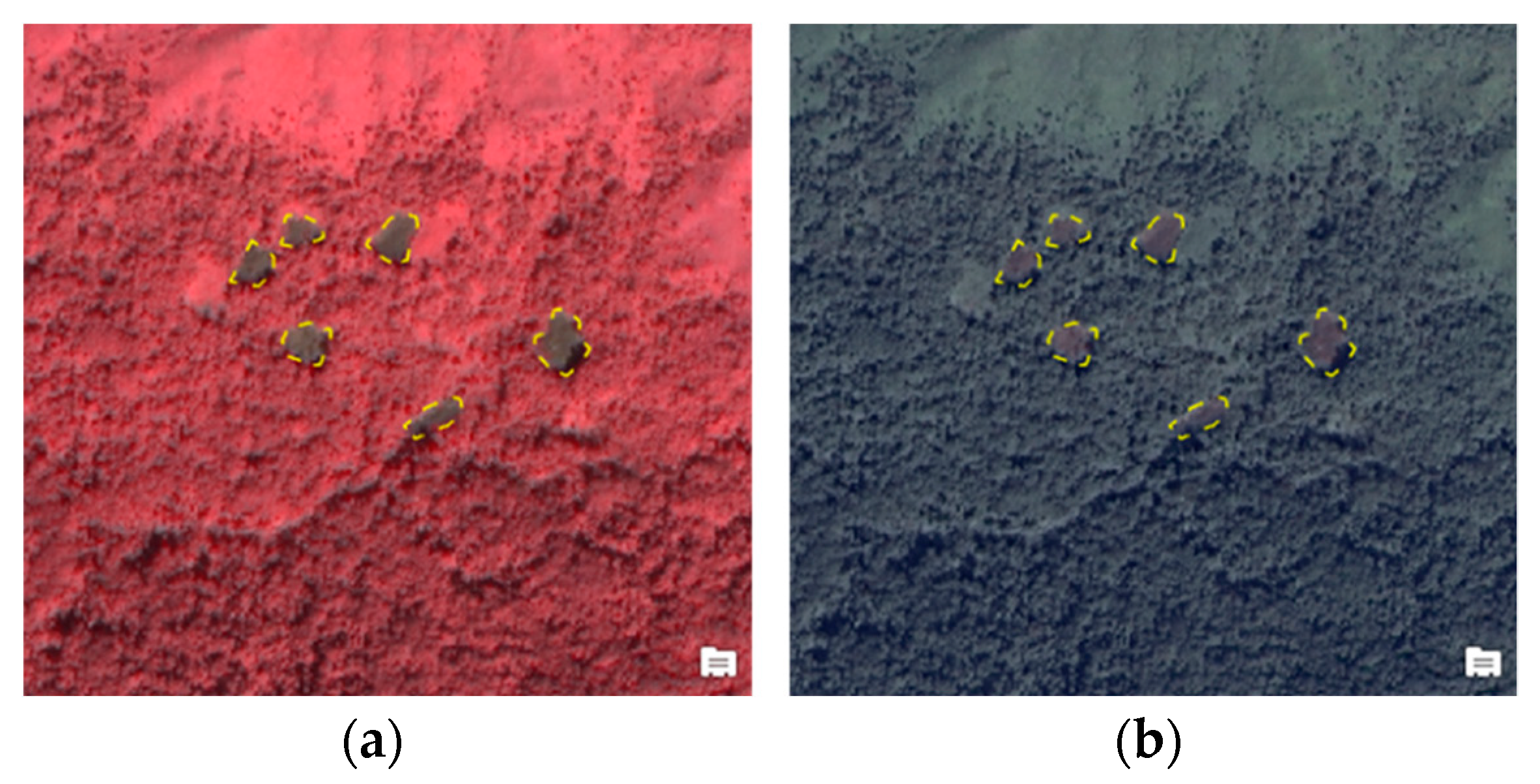
Under visible light, vegetation is usually green. A remote sensing image not only detects ground objects in visible light, it also captures near infrared or even far infrared information. Some ground object information features will be more obvious when false color synthesis is used with near infrared–red–green, and the vegetation will appear as red on the false color image. The display effects of our remote sensing images in both false-color and true-color modes are illustrated in Figure 9. We used the initial weight provided by SSD for transform learning; however, the weight parameters of the SSD model were trained using natural images in RGB mode. In order to study whether this model can learn the features of the false-color image and whether it can be used in recognition tasks, we conducted the following comparison experiment.
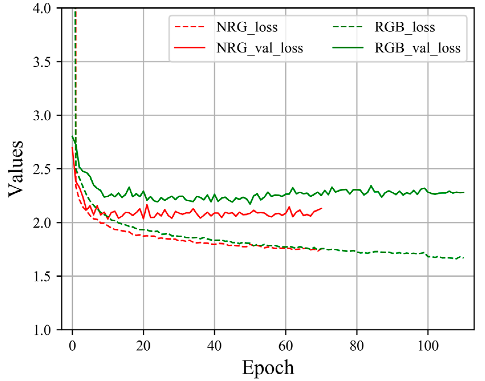
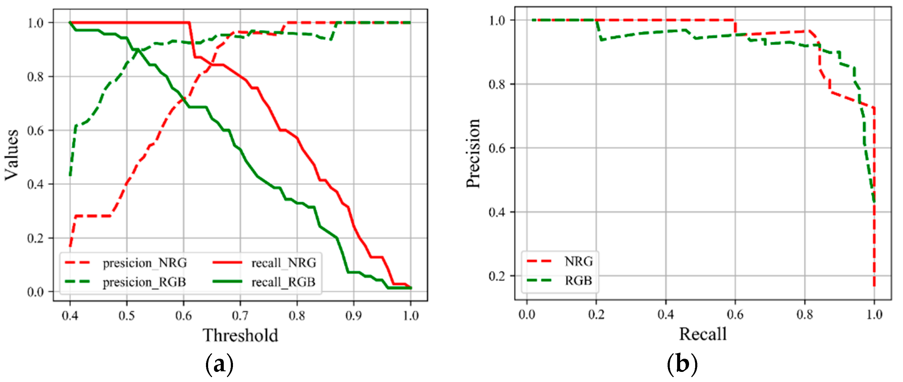
In order to reduce the influence of other factors on the experimental results, we kept the same values for the other parameters. When generating the training sample, we set the overlap parameter to 100 pixels. For the same study area, two sets of training datasets were generated using the NRG combination and the RGB combination. The number of samples in both training sets was the same (6547). The loss–decline curve of both dataset groups showed some differences during the training process. For the NRG datasets, the model achieved the lowest valid loss after approximately 10 epochs, after which it fluctuated but was generally stable. For RGB datasets, the lowest valid loss was achieved after 50 epochs. The minimum valid loss of the NRG datasets was lower than that of the RGB datasets. Thus, the true-color datasets were more difficult to train than the false-color datasets. The loss–decline curve of the two groups’ data during the training process is shown in Figure 10.
The performance of the two dataset groups on the verification image is shown in Figure 11. The precision rate of NRG is lower than that of RGB only when the threshold is less than 0.68; if the threshold is greater than 0.68, NRG precision is higher than RGB precision. The NRG recall rate is always higher than that of RGB. Regarding the precision–recall curve, the NRG is slightly better than the RGB. When the recall rate is 83%, the accuracy of the false-color model reaches 95%, whereas the accuracy of the true-color model is only 92%.
3.3. Poppy Parcel Mapping Using Optimal Results
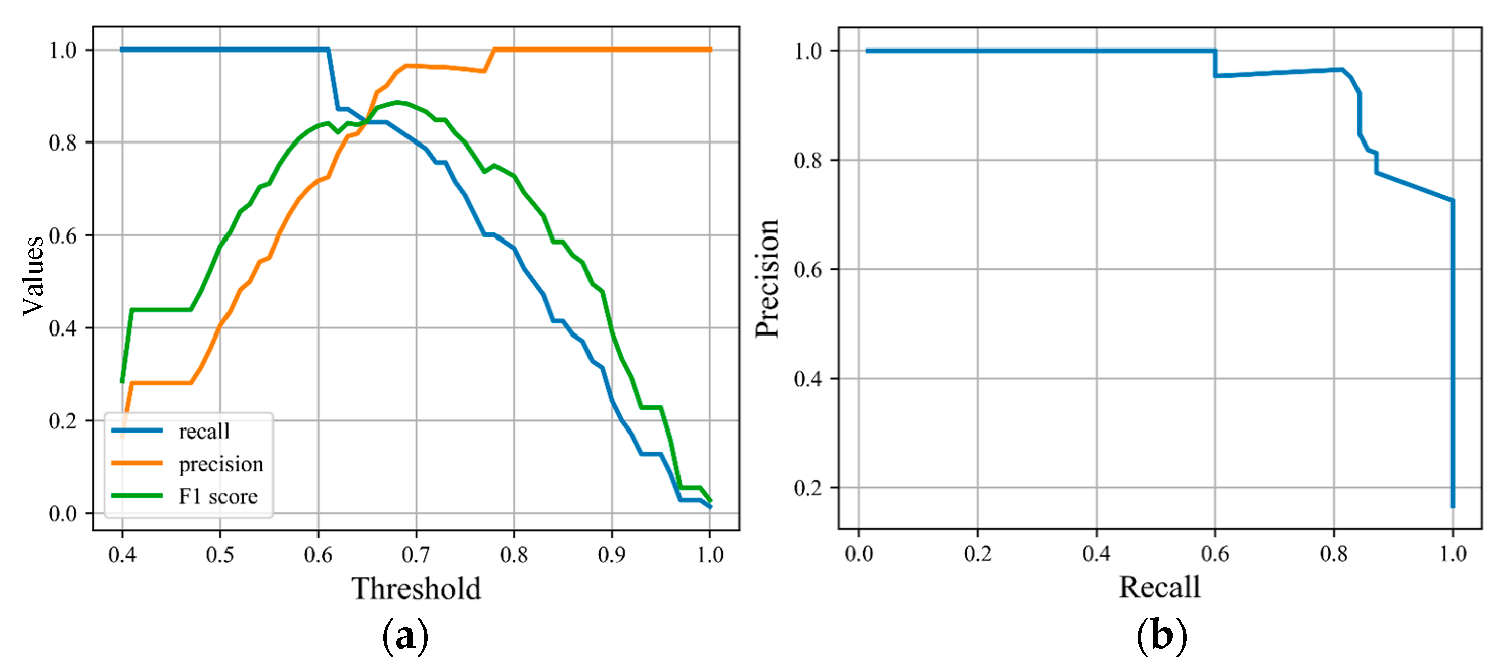
Through the experiments above, we selected the best model by using the NRG combination and an overlap of 100. We identified poppy fields in a verification image of the study area measuring 225 km2 and employed 50 s on a Windows 10 operation system with NVIDIA GTX 1080TI GPU, which allowed us to detect 4.5 km2 each second. As shown in Figure 12, the precision increases while the recall rate decreases as the confidence threshold increases. The F1 score first increases and then decreases; it reaches a maximum value of 0.89 when the confidence threshold is 0.68. At this confidence threshold, the precision reaches 95.1%, and the recall is 83%. The precision reaches 75% when the recall is 100%, and the recall reaches 83% when the precision is greater than 95%.
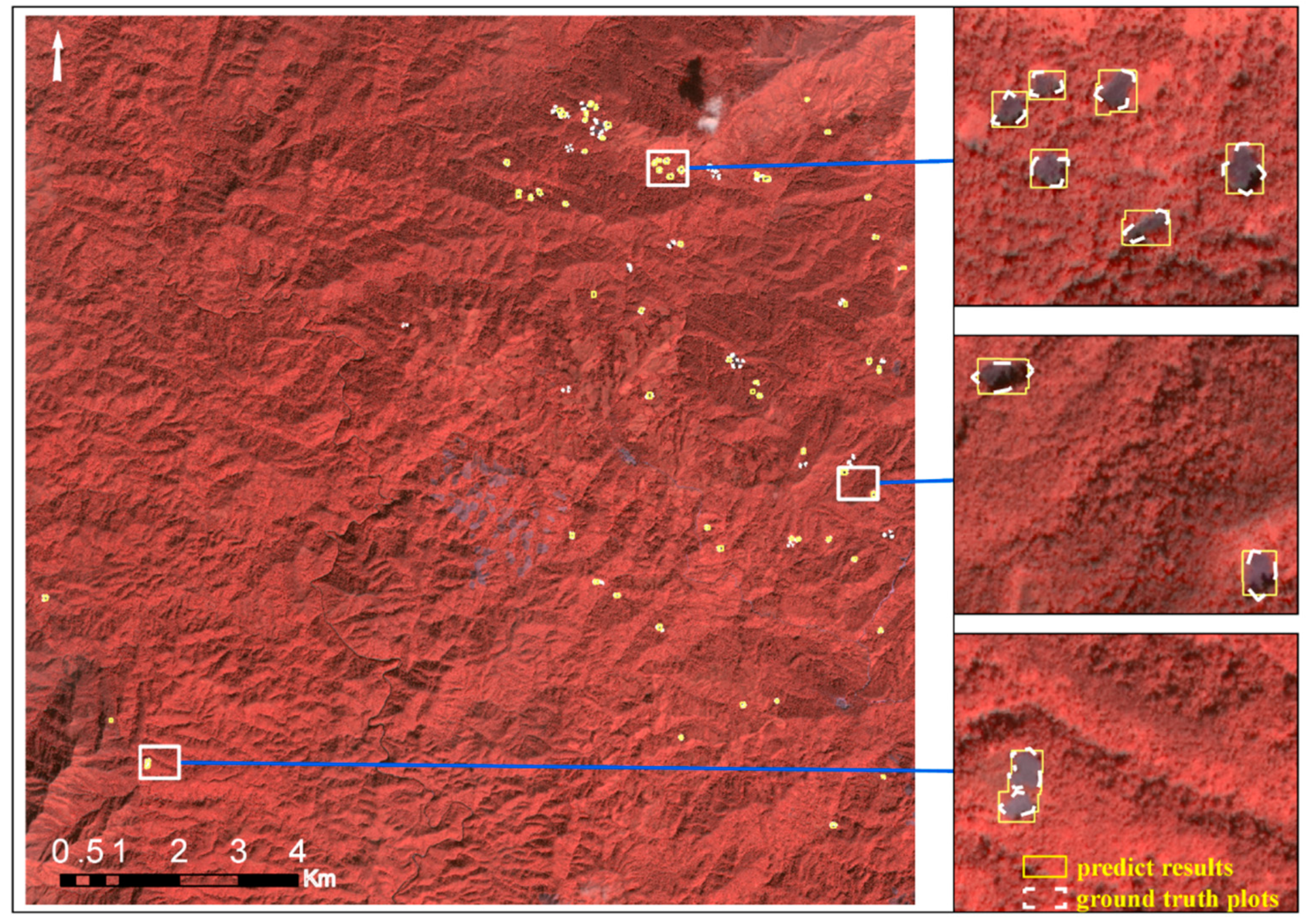
After setting the confidence threshold value to 0.68 (maximum F1 score), we generated a spatial distribution map of the opium poppy parcels in the study area. The comparison between the predicted results and the ground truth parcels of the verification image are shown in Figure 13, where the yellow rectangles are the predicted results, and the white polygons are the ground truth parcels. This spatial distribution map indicates that our model can effectively detect poppy parcels in both dense and sparse areas.
3.4. Application to Different Spatial Resolutions
Our model took 20 ms to detect each patch image measuring 300 pixels × 300 pixels. For a region with a fixed area, the number of image pixels varies with the spatial resolution, which can be approximately calculated by Formula (6), where Numbers represents the total number of pixels, W and H are the region width and length, respectively, and Res represents the image spatial resolution. When setting the overlap (default = 150) during prediction, the total time required can be calculated by Formula (7), where Speed is the time required to detect each patch image:
To explore the detection performance for different spatial resolution images, we resized our verification remote sensing image to 1.5 m, 2.0 m, 2.5 m, 3.0 m, 3.5 m, and 4.0 m, as shown in Figure 14.
Although the differences between pictures are small, the prediction results are quite different. The calculated precision–recall curves are shown in Figure 15. The accuracy does not decline substantially for resolutions of 2.5 m and 3.0 m, but the results are considerably worse at resolutions of 1.5 m, 3.5 m, and 4.0 m.
For a quantitative analysis, we set the recall rate to 83%; the precision and prediction time of different resolutions are shown in Table 5. As the resolution decreases, the precision rate also decreases, except for a resolution of 1.5 m, when the precision is minimum. The prediction times also decrease dramatically with resolution.
3.5. Application to Other Satellite Images
Our model was trained using ZY3 satellite data with two-meter resolution; therefore, we decided to verify model performance using other types of satellite images. If our model also performs well on these, it can be used to monitor an entire region with different satellite images. In order to test the generalization performance of the model, we conducted a prediction experiment on the GF-2 satellite image. GF-2 can provide 0.8-m panchromatic and 3.2-m multispectral images; we selected the 3.2-m multispectral data of the GF-2 satellite image obtained on 11 November 2017, which is also located in Phongsali province. We used our optimal model to detect poppy parcels in the GF-2 image and obtained the spatial distribution maps of poppy parcels, as shown in Figure 16.
The distribution of poppy parcels is relatively dense on the left of the image and relatively sparse in the middle part. We randomly selected eight points and generated a zoomed-in display. The model produced a good prediction for both the dense and sparse areas. This also indicates that our model has good generalization capability for poppy parcel identification, and can be directly used to identify parcels with GF-2 multi-spectral 3.2-m images.
4. Discussion
4.1. Unique Poppy Parcel Detection with Deep Learning-Based Object Detection
Monitoring poppy cultivation by remote sensing images has been indispensable, especially in Afghanistan and the Golden Triangle. The UNODC uses a statistical sample method combined with remote sensing images to estimate poppy cultivation in monitoring areas. The existing methods [4,6,7] focus almost entirely on the total planting acreage in some provinces and countries. The total planting acreage is an important indicator in evaluating the overall planting situation; however, in practice, obtaining poppy parcel location information is more important for eradicating poppies [5]. So, we put forward a new perspective that focuses on the coordinates of poppy parcels. Until now, the most highly researched regions have been in Afghanistan, with only a few in the Golden Triangle. The poppy planting situation in Lao PDR is completely different from that in Afghanistan, most notably because the majority of opium poppies are planted in the mountains, which are far from main roads and residential areas [36]. In these areas, the method used in Afghanistan is not always effective. Therefore, we proposed a new methodology to detect opium poppy parcel location coordinates in Lao PDR. Our work is the first attempt to solve the monitoring poppy problem with the object detection method, and has three major advantages. First, using the deep learning method, our method can automatically extract poppy parcel features without the need for manual selection and with a much faster detection speed. Second, the object detection method is more effective for detecting poppy parcel location information in Lao PDR because of the unique planting characteristics. Third, we conducted many comparison experiments and analyzed the effect on different parameters.
4.2. Uncertainty Analysis and Scope for Future Work
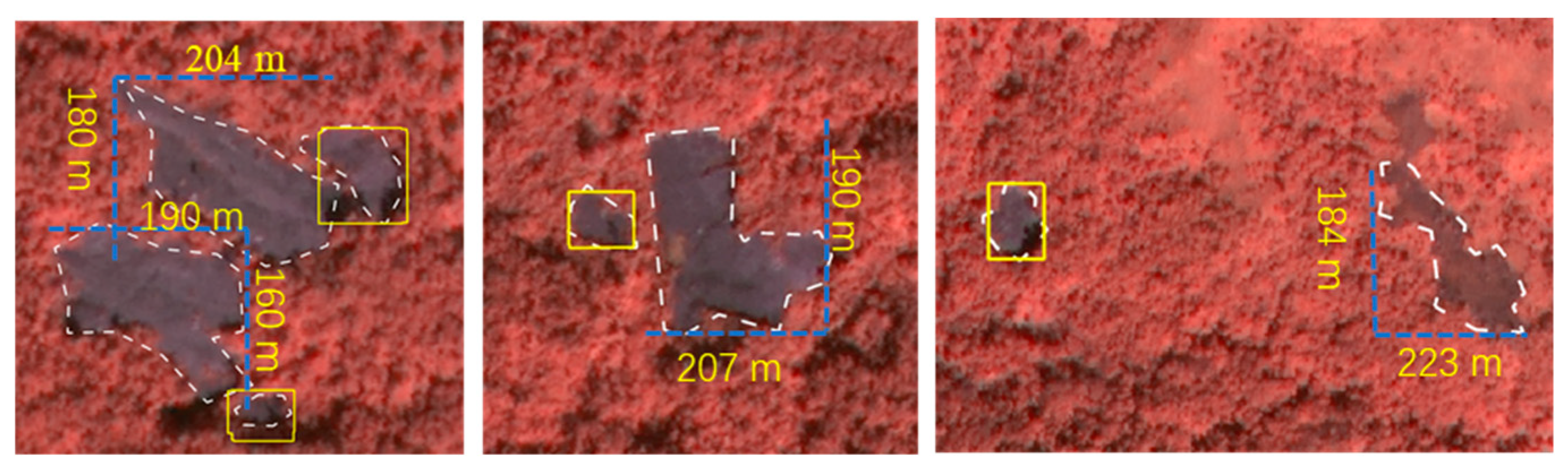
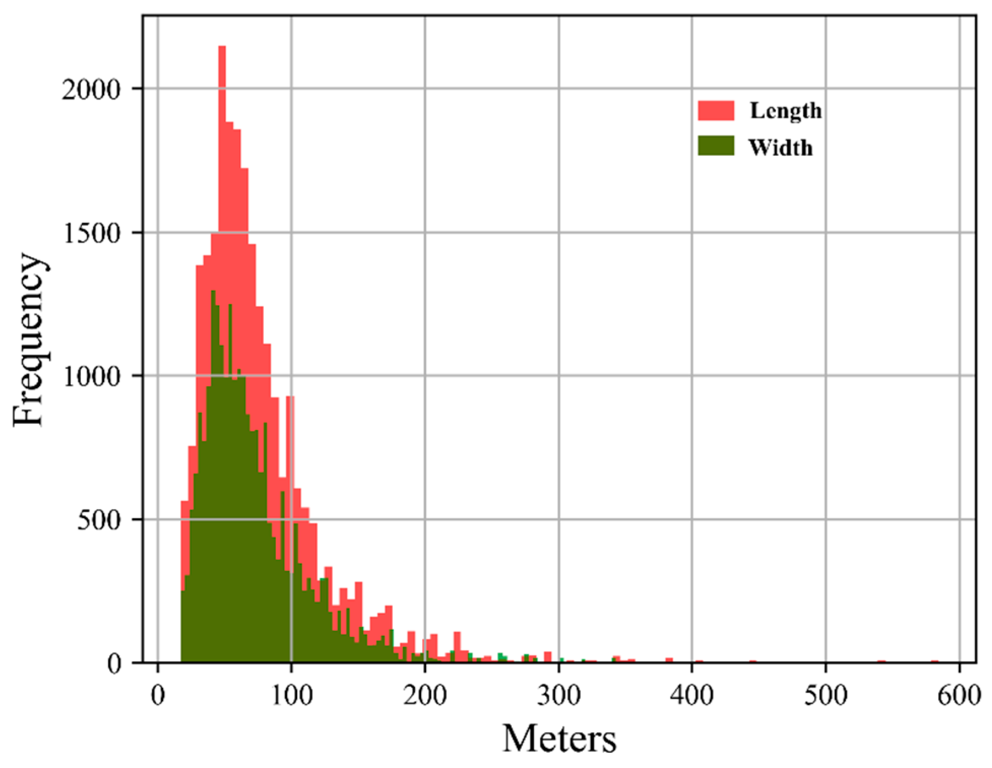
As shown from the results, when the confidence threshold is set to 0.68, the precision reaches 95.1%, yet the recall is only 83%. A potential reason for this is that our model is not good at recognizing large parcels (Figure 17). We analyzed poppy parcel samples in the training datasets and made histogram statistics of the length and width of label boxes (Figure 18); the lengths are approximately 17–400 m, and their widths are 15–263 m. For parcels larger than 150 m, there are far fewer training samples, accounting for only 7% of all samples. Therefore, these would be judged as non-poppy parcels at the prediction stage. In future work, we intend to perform a sample balancing operation and increase the number of large targets when generating training samples, allowing these features to be learned sufficiently, thereby improving the detection recall rate.
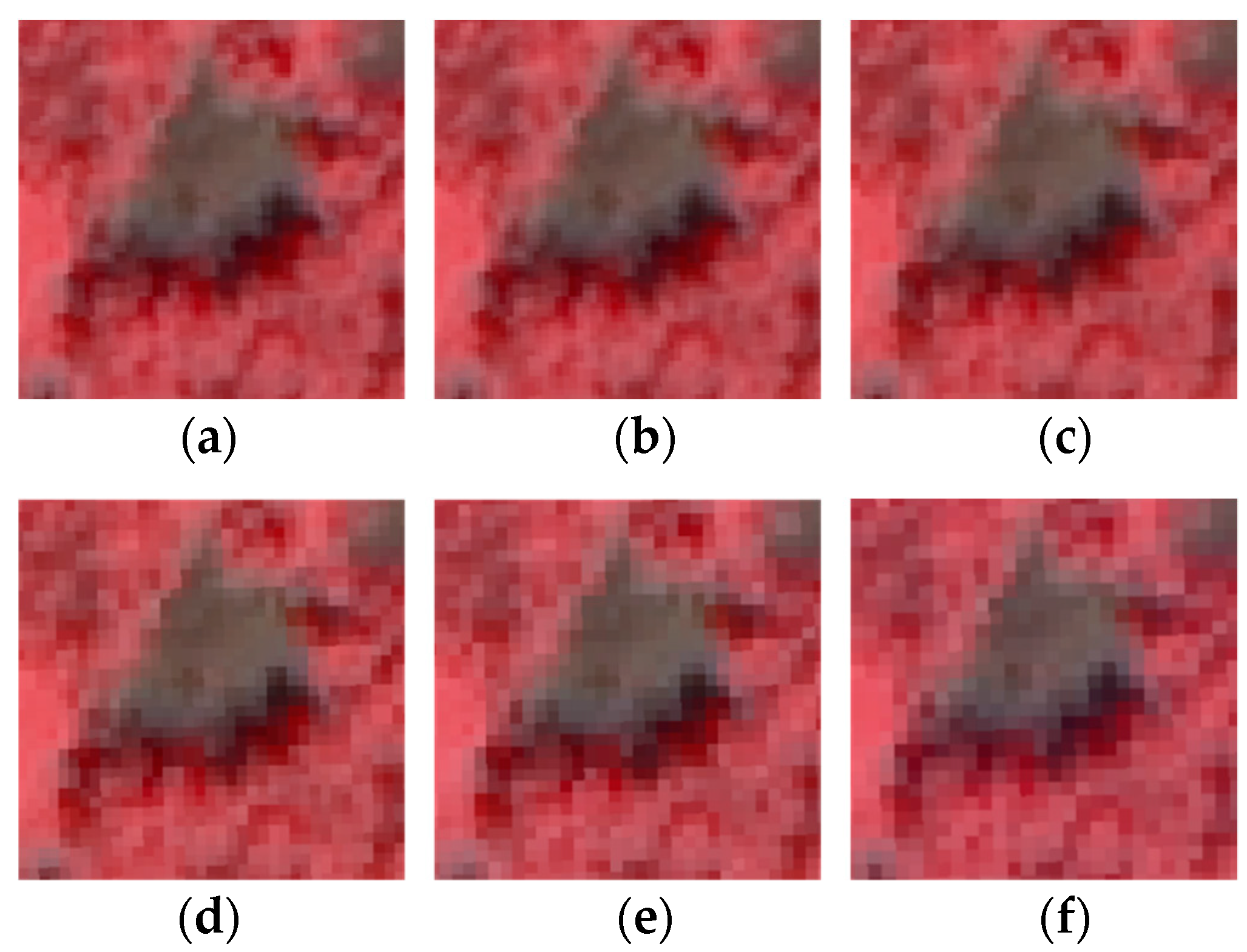
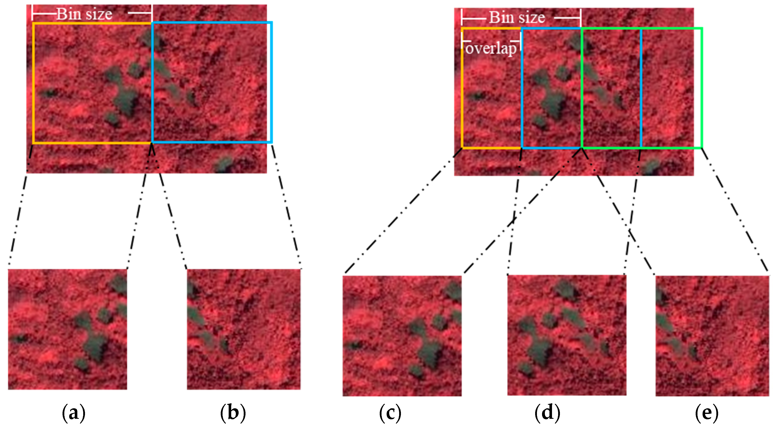
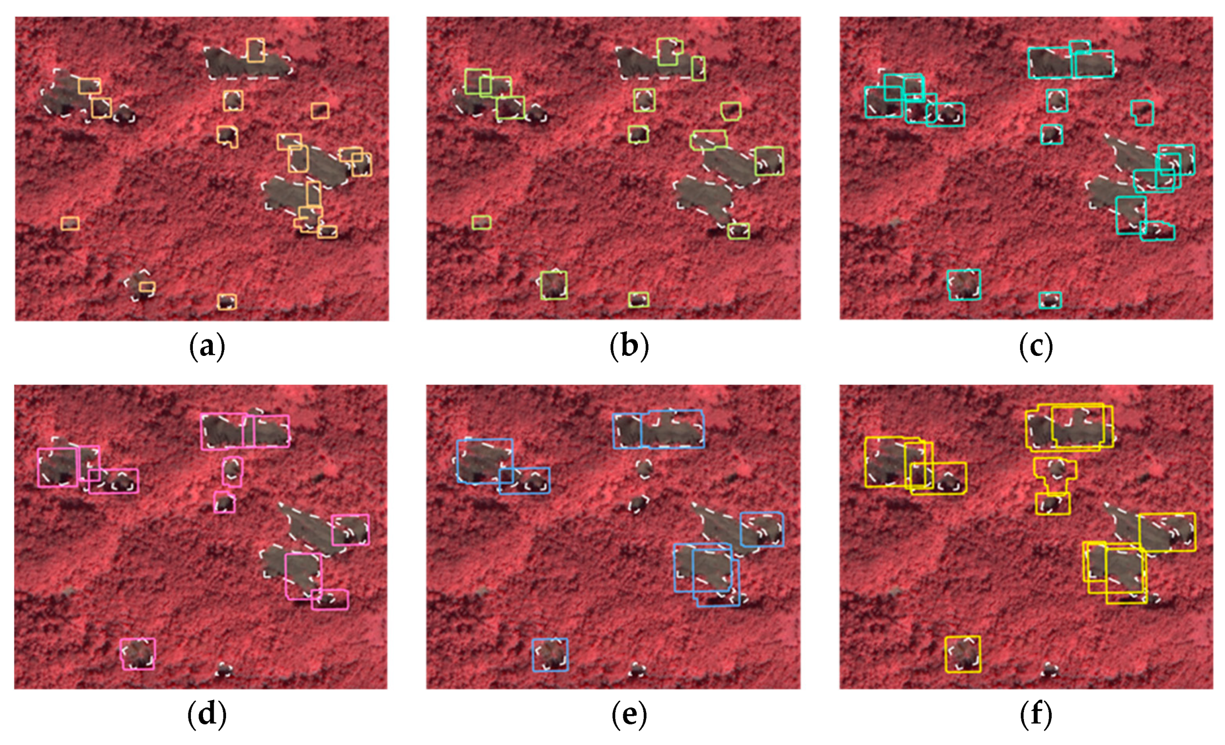
In our experiment, we found that different sliding window settings (overlap) in the training samples affected the performance of the model. An overlap of 100 produced better model performance than 150 and 200. There are two reasons that explain this phenomenon. First, not setting an overlap generates poor samples when the target is at the edge of the image (Figure 19a,b); namely, some poppy parcel features are cut. When we set an appropriate value for the overlap (Figure 19c–e), the poppy parcel features are retained (Figure 19d). In other words, using the overlap method increases the diversity of the samples.
Second, the overlap influences the number of samples. For a large remote sensing image, we can theoretically have many overlap settings. Different overlap settings will generate different amounts of training samples, and the number of samples cut can be approximately represented by Formula (8), where Trainnumber represents the number of all of the samples, Imagerows and Imagecolumns represent the number of row and column pixels in the remote sensing image, respectively, and overlap represents the size of the sliding window (an integer from one to 300).
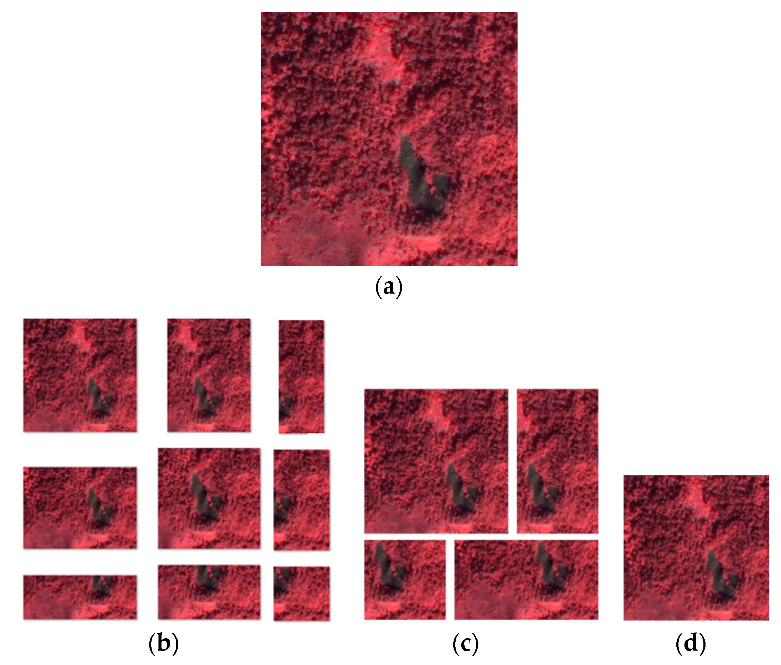
For an original image measuring 320 × 317 (Figure 20a), when the overlap is set to 100, it can be partitioned into nine different samples (Figure 20b), when it is set to 150, it can generate four samples (Figure 20c), and when it is set to 200, only one sample can be made (Figure 20d).
For every ground truth target, the small overlap setting can generate many samples with different backgrounds, which increases the diversity of the training samples. More samples often improve the performance of the deep learning model. In this study, we only conducted three comparative experiments for different overlaps. If we had set the overlap smaller, more samples would have been generated, which may improve the model performance or not. In future work, we will explore how the overlap influences the model performance, as well as whether setting it to smallest (value = 1) is the optimal choice.
Deep learning-based object detection requires three-band pictures, whereas the remote sensing images employed contain four bands (near infrared–red–green–blue), so we can only choose three of the four bands. In our study, we used false-color (NRG) and true-color (RGB) for the training datasets. Our results showed that the model trained on NRG datasets performed better than that on RGB datasets, which also proved that false-color synthetic images using the NRG band can be continually trained based on the initial weight of SSD. Since the images utilized the information of the near infrared band, which is sensitive to vegetation, the recognition accuracy for poppy parcels was improved. We only trained the model using NRG and RGB, yet there are 24 different combinations of four band images, such as 4-3-1, 4-2-1, 4-1-3, etc. More experiments need to be conducted in order to explore the best band combination. Besides, we cannot utilize all four bands, because remote sensing fields do not contain millions of labeled datasets [41], so we have to abandon some band information when using a pre-trained model. On the other hand, the saliency map based on SAR images has been used to detect targets [42,43,44], which provide a novel research direction. In future work, we intend to conduct some experiments to explore if the opium poppy parcels have unique characteristics compared with the surrounding environment (forests and farmland) in SAR images, and we intend to explore the saliency map of the opium poppy parcels and use the saliency map as an input of the SSD model. We also intend to design a new deep convolutional neural network to take advantage of remote sensing multi-band information on optical images and the saliency map on SAR images.
We also explore our model performance (trained at 2.0 m) on different spatial resolution images and other types of satellite image. As the results show, when our model predicts poppy parcels on images with spatial resolutions of 2.5 m and 3.0 m, their precision only declines by 7% for the same recall, but the prediction time is greatly reduced, resulting in a rapid detection method. When we set the confidence threshold to 0.56, the detection performance is good for large parcels at resolutions of 4.0 m and 3.5 m (Figure 21), but it is poor for small parcels. When the resolution is close to 2.0 m (2.5 m or 3.0 m), it can detect a majority of both large and small parcels, but contains several superfluous prediction boxes, which result in lower precision compared with a resolution of 2.0 m. When the resolution is higher (1.5 m), the prediction box size is much smaller, which reduces the prediction accuracy. In conclusion, a slightly lower resolution than that trained on the model can result in a better prediction. Thus, in future work, we will attempt to train a single model using different resolution images, which may result in a better generalization performance.
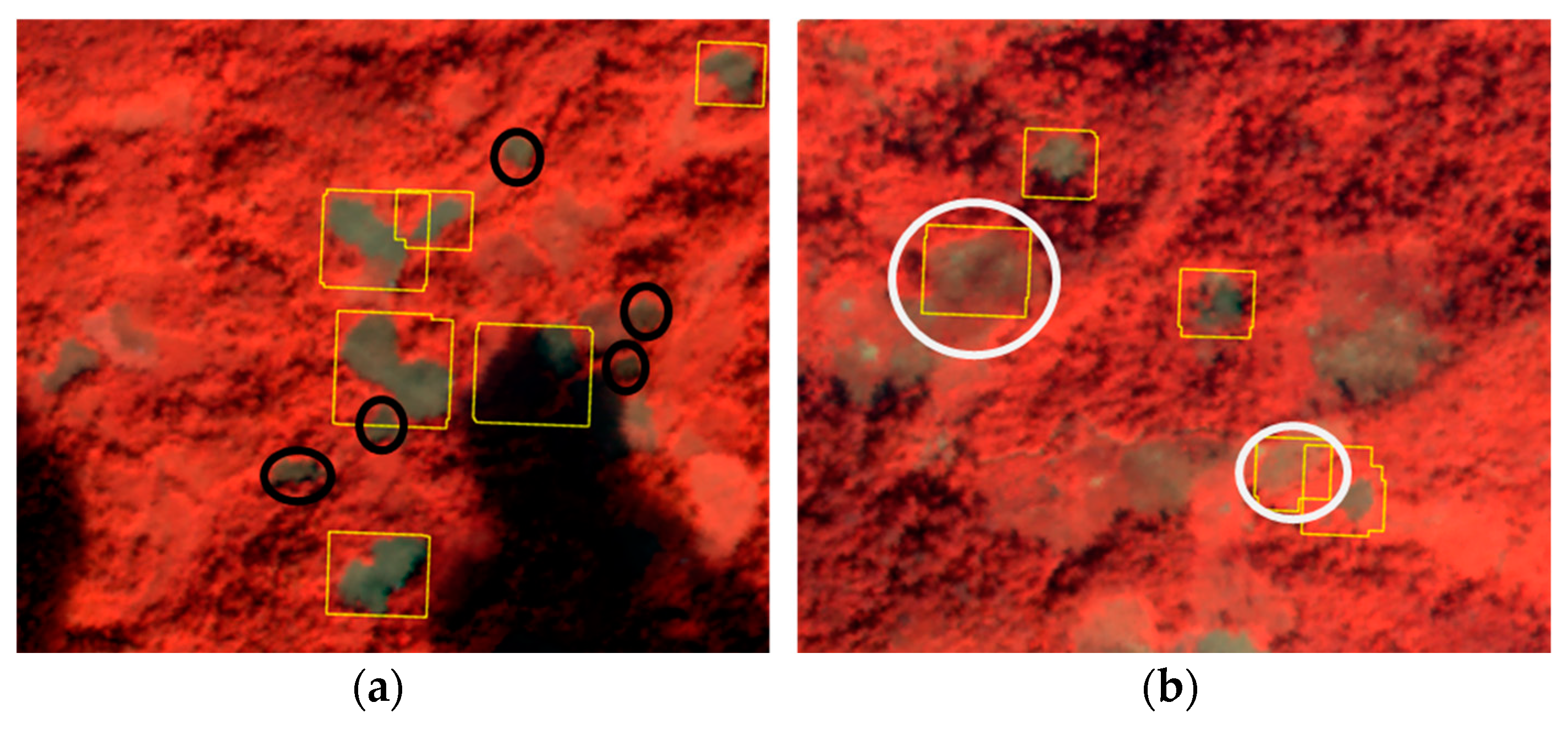
We also proved that our model is effective for GF-2 multispectral images. However, some small poppy parcels of approximately 10 pixels could not be detected in the 3.2-m image (Figure 22a), and some agriculture parcels were detected incorrectly (Figure 22b).
To improve the model for different satellite images, we aim to more effectively train the model using combinations of other satellite images. Furthermore, as we only conducted experiments on GF-2 images, more research is required on other types of remote sensing images.
5. Conclusions
Using satellite remote sensing has become a mainstream approach for monitoring poppy cultivation. However, identifying the location of poppy parcels and mapping their spatial distribution are of great practical significance for local governments making and implementing eradication plans. In order to obtain the specific location coordinates of poppy parcels, we used deep learning-based object detection to detect the location of target poppy parcels in remote sensing images and obtain a spatial distribution map of the poppy growing area. We also compared and analyzed the model performance in different situations using verification areas in Phongsali. It was found that for the region in Phongsali, our method can not only detect poppy parcel locations with a higher precision and recall (95% and 85%, respectively), it also performs well on other types of satellite images and at other spatial resolutions. Compared to existing monitoring methods, our work has three unique points: (1) it can obtain the specific location coordinates of poppy parcels by automatic feature extraction from training data; (2) it provides a quantitative analysis of prediction performance for different parameters; and (3) it performs well on satellite images of different types and varying spatial resolution. In future work, our detection method will be utilized to monitor poppy parcels in different areas, and more experiments will be conducted to verify the applicability of our model to other types of satellite images.
Author Contributions
Y.T. and C.Y. proposed the framework of detection poppy. X.L. performed the experiments and write the paper, F.Z. and G.Y. performed the data collection and analysis and revised the paper.
Funding
This research was funded by National Key R&D Program of China (2016 YFC0800901) and “The Opium Poppy Cultivation Monitoring and Eradication Program (OPCMEP)” from the Chinese National Narcotics Control Commission (CNNCC).
Acknowledgments
The authors would like to thank Like Yu for fruitful discussions on paper’s structure, at the same time, we thank the editor-in-chief, the anonymous reviewers for their systematic review and valuable comments.
Conflicts of Interest
The authors declare no conflict of interest.
Abbreviations
The following abbreviations are used in this manuscript:
| UNODC | United Nations Office on Drugs and Crime |
| CNNCC | Chinese National Narcotics Control Commission |
| RGB | Red–Green–Blue |
| NRG | Near infrared-Red-Green |
| VGG | Visual Geometry Group |
| DCNN | Deep Convolutional Neural Network |
| SSD | Single Shot Multibox Detector |
References
- Agrawal, S.; Joshi, P.; Shukla, Y.; Roy, P. Spot vegetation multi temporal data for classifying vegetation in south central Asia. Curr. Sci. 2003, 84, 1440–1448. [Google Scholar]
- Wang, L.; Sousa, W.; Gong, P. Integration of object-based and pixel-based classification for mapping mangroves with IKONOS imagery. Int. J. Remote Sens. 2004, 25, 5655–5668. [Google Scholar] [CrossRef]
- Chuinsiri, S.; Blasco, F.; Bellan, M.; Kergoat, L. A poppy survey using high resolution remote sensing data. Int. J. Remote Sens. 1997, 18, 393–407. [Google Scholar] [CrossRef]
- UNODC. World Drug Report 2005. Available online: http://www.unodc.org /unodc/ en/data-and-analysis/WDR-2005.html (accessed on 16 October 2018).
- Tian, Y.; Wu, B.; Zhang, L.; Li, Q.; Jia, K.; Wen, M. Opium poppy monitoring with remote sensing in North Myanmar. Int. J. Drug Policy 2011, 22, 278–284. [Google Scholar] [CrossRef] [PubMed]
- Simms, D.M.; Waine, T.W.; Taylor, J.C. Improved estimates of opium cultivation in Afghanistan using imagery-based stratification. Int. J. Remote Sens. 2017, 38, 3785–3799. [Google Scholar] [CrossRef]
- Simms, D.M.; Waine, T.W.; Taylor, J.C.; Brewer, T.R. Image segmentation for improved consistency in image-interpretation of opium poppy. Int. J. Remote Sens. 2016, 37, 1243–1256. [Google Scholar] [CrossRef]
- Jia, K.; Wu, B.; Tian, Y.; Li, Q.; Du, X. Spectral discrimination of opium poppy using field spectrometry. IEEE Trans. Geosci. Remote Sens. 2011, 49, 3414. [Google Scholar] [CrossRef]
- Wang, J.-J.; Zhang, Y.; Bussink, C. Unsupervised multiple endmember spectral mixture analysis-based detection of opium poppy fields from an EO-1 Hyperion image in Helmand, Afghanistan. Sci. Total Environ. 2014, 476, 1–6. [Google Scholar] [CrossRef] [PubMed]
- Wang, J.-J.; Zhou, G.; Zhang, Y.; Bussink, C.; Zhang, J.; Ge, H. An unsupervised mixture-tuned matched filtering-based method for the remote sensing of opium poppy fields using EO-1 Hyperion data: An example from Helmand, Afghanistan. Remote Sens. Lett. 2016, 7, 945–954. [Google Scholar] [CrossRef]
- Bennington, A.L. Application of Multi-Spectral Remote Sensing for Crop Discrimination in Afghanistan. Ph.D. Thesis, Cranfield University, Bedfordshire, UK, March 2008. [Google Scholar]
- Zhou, J.; Bischof, W.F.; Caelli, T. Road tracking in aerial images based on human–computer interaction and Bayesian filtering. ISPRS-J. Photogramm. Remote Sens. 2006, 61, 108–124. [Google Scholar] [CrossRef]
- Xu, C.; Duan, H. Artificial bee colony (ABC) optimized edge potential function (EPF) approach to target recognition for low-altitude aircraft. Pattern Recognit. Lett. 2010, 31, 1759–1772. [Google Scholar] [CrossRef]
- Leninisha, S.; Vani, K. Water flow based geometric active deformable model for road network. ISPRS-J. Photogramm. Remote Sens. 2015, 102, 140–147. [Google Scholar] [CrossRef]
- Martha, T.R.; Kerle, N.; van Westen, C.J.; Jetten, V.; Kumar, K.V. Segment optimization and data-driven thresholding for knowledge-based landslide detection by object-based image analysis. IEEE Geosci. Remote Sens. Lett. 2011, 49, 4928–4943. [Google Scholar] [CrossRef]
- Baker, B.A.; Warner, T.A.; Conley, J.F.; McNeil, B.E. Does spatial resolution matter? A multi-scale comparison of object-based and pixel-based methods for detecting change associated with gas well drilling operations. Int. J. Remote Sens. 2013, 34, 1633–1651. [Google Scholar] [CrossRef]
- Contreras, D.; Blaschke, T.; Tiede, D.; Jilge, M. Monitoring recovery after earthquakes through the integration of remote sensing, GIS, and ground observations: the case of L’Aquila (Italy). Cartogr. Geogr. Inf. Sci. 2016, 43, 115–133. [Google Scholar] [CrossRef]
- Kembhavi, A.; Harwood, D.; Davis, L.S. Vehicle detection using partial least squares. IEEE Trans. Pattern Anal. Mach. Intell. 2011, 33, 1250–1265. [Google Scholar] [CrossRef] [PubMed]
- Aytekin, Ö.; Zöngür, U.; Halici, U. Texture-based airport runway detection. IEEE Geosci. Remote Sens. Lett. 2013, 10, 471–475. [Google Scholar] [CrossRef]
- Zhao, Y.-Q.; Yang, J. Hyperspectral image denoising via sparse representation and low-rank constraint. IEEE Geosci. Remote Sens. Lett. 2015, 53, 296–308. [Google Scholar] [CrossRef]
- Cheng, G.; Han, J. A survey on object detection in optical remote sensing images. ISPRS-J. Photogramm. Remote Sens. 2016, 117, 11–28. [Google Scholar] [CrossRef] [Green Version]
- Simonyan, K.; Zisserman, A. Very deep convolutional networks for large-scale image recognition. arXiv, 2014; arXiv:1409.1556. Available online: https://arxiv.org/abs/1409.1556 (accessed on 16 October 2018).
- Krizhevsky, A.; Sutskever, I.; Hinton, G.E. Imagenet classification with deep convolutional neural networks. In Proceedings of the Advances in Neural Information Processing Systems, Lake Tahoe, NV, USA, 3–6 December 2012; pp. 1097–1105. [Google Scholar]
- Szegedy, C.; Liu, W.; Jia, Y.; Sermanet, P.; Reed, S.; Anguelov, D.; Erhan, D.; Vanhoucke, V.; Rabinovich, A. Going deeper with convolutions. In Proceedings of the IEEE Conference on Computer Vision and Pattern Recognition, Columbus, OH, USA, 23–28 June 2014; pp. 1–9. [Google Scholar]
- Costante, G.; Ciarfuglia, T.A.; Biondi, F. Towards Monocular Digital Elevation Model (DEM)Estimation by Convolutional Neural Networks—Application on Synthetic Aperture Radar Images. In Proceedings of the European Conference on Synthetic Aperture Radar, Aachen, Germany, 4–7 June 2018; pp. 1–6. [Google Scholar]
- Zhang, L.; Xia, G.-S.; Wu, T.; Lin, L.; Tai, X.C. Deep learning for remote sensing image understanding. J. Sens. 2016, 501. [Google Scholar] [CrossRef]
- Girshick, R. Fast r-cnn. In Proceedings of the IEEE International Conference on Computer Vision, Santiago, Chile, 7–13 December 2015; pp. 1440–1448. [Google Scholar]
- Girshick, R.; Donahue, J.; Darrell, T.; Malik, J. Rich feature hierarchies for accurate object detection and semantic segmentation. In Proceedings of the IEEE Conference on Computer Vision and Pattern Recognition, Columbus, OH, USA, 23–28 June 2014; pp. 580–587. [Google Scholar]
- Ren, S.; He, K.; Girshick, R.; Sun, J. Faster r-cnn: Towards real-time object detection with region proposal networks. In Proceedings of the Advances in Neural Information Processing Systems, Montreal, Canada, 7–12 December 2015; pp. 91–99. [Google Scholar]
- Redmon, J.; Divvala, S.; Girshick, R.; Farhadi, A. You only look once: Unified, real-time object detection. In Proceedings of the IEEE Conference on Computer Vision and Pattern Recognition, Seattle, WA, USA, 27–30 June 2016; pp. 779–788. [Google Scholar]
- Liu, W.; Anguelov, D.; Erhan, D.; Szegedy, C.; Reed, S.; Fu, C.-Y.; Berg, A.C. Ssd: Single shot multibox detector. In Proceedings of the European Conference on Computer Vision, Amsterdam, The Netherlands, 8–16 October 2016; pp. 21–37. [Google Scholar]
- Ye, Q.; Huo, H.; Zhu, T.; Fang, T. Harbor Detection in Large-Scale Remote Sensing Images Using Both Deep-Learned and Topological Structure Features. In Proceedings of the Computational International Symposium on Computational Intelligence and Design, Hangzhou, China, 9–10 December 2017; pp. 218–222. [Google Scholar]
- Marcum, R.A.; Davis, C.H.; Scott, G.J.; Nivin, T.W. Rapid broad area search and detection of Chinese surface-to-air missile sites using deep convolutional neural networks. J. Appl. Remote Sens. 2017, 11, 042614. [Google Scholar] [CrossRef]
- Wang, Y.; Wang, C.; Zhang, H.; Zhang, C.; Fu, Q. Combing Single Shot Multibox Detector with transfer learning for ship detection using Chinese Gaofen-3 images. In Proceedings of the Progress in Electromagnetics Research Symposium, Toyama, Japan, 1–4 August 2017; pp. 712–716. [Google Scholar]
- Zhang, Y.; Fu, K.; Sun, H.; Sun, X.; Zheng, X.; Wang, H. A multi-model ensemble method based on convolutional neural networks for aircraft detection in large remote sensing images. Remote Sens. Lett. 2018, 9, 11–20. [Google Scholar] [CrossRef]
- Chinese National Narcotics Control Commission (CNNCC). Opium Poppy Monitoring in Laos. (Interior Material), Beijing: CNNCC, 2017. Available online: http://www.nncc.org.cn/ (accessed on 16 October 2018).
- Liu, X.; Feng, Z.; Jiang, L.; Li, P.; Liao, C.; Yang, Y.; You, Z. Rubber plantation and its relationship with topographical factors in the border region of China, Laos and Myanmar. J. Geogr. Sci. 2013, 23, 1019–1040. [Google Scholar] [CrossRef]
- Prapinmongkolkarn, P.; Thisayakorn, C.; Kattiyakulwanich, N.; Murai, S.; Kittichanan, H.; Vanasathid, C.; Okuda, T.; Jirapayooungchai, K.; Sramudcha, J.; Matsuoka, R. Remote sensing applications to land cover classification in northern Thailand [LANDSAT]. J. Biol. Chem. 2015, 270, 10828–10832. [Google Scholar]
- Hu, F.; Xia, G.-S.; Hu, J.; Zhang, L. Transferring deep convolutional neural networks for the scene classification of high-resolution remote sensing imagery. Remote Sens. 2015, 7, 14680–14707. [Google Scholar] [CrossRef]
- Huang, B.; Zhao, B.; Song, Y. Urban land-use mapping using a deep convolutional neural network with high spatial resolution multispectral remote sensing imagery. Remote Sens. Environ. 2018, 214, 73–86. [Google Scholar] [CrossRef]
- Ester, M.; Kriegel, H.P.; Xu, X. A density-based algorithm for discovering clusters a density-based algorithm for discovering clusters in large spatial databases with noise. In Proceedings of the International Conference on Knowledge Discovery and Data Mining, Portland, OR, USA, 4–8 August 1996; pp. 226–231. [Google Scholar]
- Zhu, D.; Wang, B.; Zhang, L. Airport target detection in remote sensing images: A new method based on two-way saliency. IEEE Geosci. Remote Sens. Lett. 2015, 12, 1096–1100. [Google Scholar]
- Tu, S.; Su, Y. Fast and accurate target detection based on multiscale saliency and active contour model for high-resolution SAR images. IEEE Trans. Geosci. Remote Sens. 2016, 54, 5729–5744. [Google Scholar] [CrossRef]
- Karine, A.; Toumi, A.; Khenchaf, A.; EL Hassouni, M. Radar Target Recognition using Salient Keypoint Descriptors and Multitask Sparse Representation. Remote Sens. 2018, 10, 843. [Google Scholar] [CrossRef]
Figure 1.
Differences in opium poppy fields between (a) Afghanistan and (b) Lao PDR.

Figure 2.
Workflow of the method: (a) diagram of the methodological framework, (b) a detailed description of the single shot multibox detector (SSD) architecture.
Figure 2.
Workflow of the method: (a) diagram of the methodological framework, (b) a detailed description of the single shot multibox detector (SSD) architecture.

Figure 3.
Location of the study area. The region marked by pink lines is Phongsali province; the pink rectangle represents the area used for verification, and the green polygon represents the area used for training.
Figure 3.
Location of the study area. The region marked by pink lines is Phongsali province; the pink rectangle represents the area used for verification, and the green polygon represents the area used for training.

Figure 4.
Meteorological data for north Laos: (a) number of rainy days per month, (b) temperature and precipitation per month; lines represent temperature, and histogram represents rainfall. Data source: World Meteorological Organization statistics for approximately 30 years. (http://worldweather.wmo.int/en/city.html?cityId=1501).

Figure 5.
Partitioning of the entire image into smaller fragments via the sliding window. The bin size was set to 300 pixels × 300 pixels, and the overlap was set to 150 pixels.
Figure 5.
Partitioning of the entire image into smaller fragments via the sliding window. The bin size was set to 300 pixels × 300 pixels, and the overlap was set to 150 pixels.

Figure 6.
Prediction frequency diagram for the whole image. Each little square represents a region with 150 pixels × 150 pixels; the numbers in the squares are the numbers of predictions, which are treated as weights to calculate the final poppy confidence.
Figure 6.
Prediction frequency diagram for the whole image. Each little square represents a region with 150 pixels × 150 pixels; the numbers in the squares are the numbers of predictions, which are treated as weights to calculate the final poppy confidence.

Figure 7.
Post-processing steps: (a) Ori-results polygons, (b) density-based clustering for center coordinate points, different colors represent different clustering classes, (c) final result after merging the same clustering.
Figure 7.
Post-processing steps: (a) Ori-results polygons, (b) density-based clustering for center coordinate points, different colors represent different clustering classes, (c) final result after merging the same clustering.

Figure 8.
Model performance with different overlaps.

Figure 9.
Illustrations of the different band combinations: (a) NRG combination image and (b) RGB combination image. Yellow dotted lines indicate the target parcels.
Figure 9.
Illustrations of the different band combinations: (a) NRG combination image and (b) RGB combination image. Yellow dotted lines indicate the target parcels.

Figure 10.
Loss curve for different band combinations.

Figure 11.
Performance of different band combinations: (a) precision and recall on different confidence thresholds, (b) precision–recall curves for different color modes.
Figure 11.
Performance of different band combinations: (a) precision and recall on different confidence thresholds, (b) precision–recall curves for different color modes.

Figure 12.
Accuracy assessment of optimal model results. (a) The recall, precision, and F1 score vary with the confidence threshold value. (b) Precision–recall curve for optimal model.
Figure 12.
Accuracy assessment of optimal model results. (a) The recall, precision, and F1 score vary with the confidence threshold value. (b) Precision–recall curve for optimal model.

Figure 13.
Spatial distribution map of opium poppy parcels in the study area, showing a comparison between predicted results (yellow line) and ground truth results (white dotted line).
Figure 13.
Spatial distribution map of opium poppy parcels in the study area, showing a comparison between predicted results (yellow line) and ground truth results (white dotted line).

Figure 14.
Verification remote sensing images at various resolutions: (a) 1.5 m, (b) 2.0 m, (c) 2.5 m, (d) 3.0 m, (e) 3.5 m, and (f) 4.0 m.
Figure 14.
Verification remote sensing images at various resolutions: (a) 1.5 m, (b) 2.0 m, (c) 2.5 m, (d) 3.0 m, (e) 3.5 m, and (f) 4.0 m.

Figure 15.
Precision–recall curves for images with different resolutions.

Figure 16.
Spatial distribution maps of poppy parcels using the GF-2 image, yellow polygons are poppy parcels predicted by the model.
Figure 16.
Spatial distribution maps of poppy parcels using the GF-2 image, yellow polygons are poppy parcels predicted by the model.

Figure 17.
An example of poor performance of the model with large parcels: the yellow rectangle boxes are prediction results, the white polygons are ground truth poppy parcels; some bigger parcels are not detected.
Figure 17.
An example of poor performance of the model with large parcels: the yellow rectangle boxes are prediction results, the white polygons are ground truth poppy parcels; some bigger parcels are not detected.

Figure 18.
Histogram of training sample lengths and widths.

Figure 19.
Images showing the benefit of using an overlap. (a,b) Poor samples when the target is at the edge of the image; (c–e) samples when set an appropriate value for the overlap, especially (d) retains the poppy parcel features.
Figure 19.
Images showing the benefit of using an overlap. (a,b) Poor samples when the target is at the edge of the image; (c–e) samples when set an appropriate value for the overlap, especially (d) retains the poppy parcel features.

Figure 20.
Training sample images showing the effect of the overlap. (a) The original image measuring 320 × 317; (b–d) the different samples when the overlap is 100, 150, and 200.
Figure 20.
Training sample images showing the effect of the overlap. (a) The original image measuring 320 × 317; (b–d) the different samples when the overlap is 100, 150, and 200.

Figure 21.
Performance of the model for different image resolutions: (a) 1.5 m, (b) 2.0 m, (c) 2.5 m, (d) 3.0 m, (e) 3.5 m, and (f) 4.0 m.
Figure 21.
Performance of the model for different image resolutions: (a) 1.5 m, (b) 2.0 m, (c) 2.5 m, (d) 3.0 m, (e) 3.5 m, and (f) 4.0 m.

Figure 22.
Prediction using the GF-2 image (3.2 m). The black circles in (a) represent small poppy parcels that were not detected, and the white circles in (b) show agriculture plots that were incorrectly judged as poppy parcels.
Figure 22.
Prediction using the GF-2 image (3.2 m). The black circles in (a) represent small poppy parcels that were not detected, and the white circles in (b) show agriculture plots that were incorrectly judged as poppy parcels.


Table 1.
Poppy calendar for North Lao PDR.
| Months | Climatic Seasons | Main Agricultural Activities |
|---|---|---|
| June–August | Almost continuous rain | Almost no poppy activity |
| September–October | End of rainy season | Slash and burn of small forest plots |
| November–February | Cool dry season, sometimes sunny | Drying the soil and sowing Weeding and thinning Blossoming Harvesting poppy capsules Burning the stubble |
| March–May | Scattered rains and beginning of the rainy season | End of harvesting season for late varieties |
Data source: Opium Poppy Monitoring in Laos 2017. Chinese National Narcotics Control Commission CNNCC).
Table 2.
Description of the satellite images. GF-2: GaoFen-2, ZY3: ZiYuan3.
| Satellite | Height | Incidence Angle | Sensor | Id-Image | Band | Wavelength (nm) |
|---|---|---|---|---|---|---|
| ZY3 | 506 km | 97.421° | MUX | ZY3_MUX_E102.5_N21.5_20161122_L1A0003584928 ZY3_MUX_E102.4_N21.1_20161122_L1A0003584929 | Near Infrared | 770–890 |
| Red | 630–690 | |||||
| Green | 520–590 | |||||
| Blue | 450–520 | |||||
| TLC | ZY3_NAD_E102.5_N21.5_20161122_L1A0003583973 ZY3_NAD_E102.4_N21.1_20161122_L1A0003583974 | Panchromatic | 500–800 | |||
| GF-2 | 631 km | 97.908° | PMS1 | GF2_PMS1_E102.1_N22.1_20171101_L1A0002729519 | Near Infrared | 770–890 |
| Red | 630–690 | |||||
| Green | 520–590 | |||||
| Blue | 450–520 |
Table 3.
Information of the six datasets. NRG: near infrared–red–green, RGB: red–green–blue.
| Color Mode | Overlap | Picture Samples | Poppy Parcels Targets |
|---|---|---|---|
| false color (NRG) | 100 | 14,559 | 24,411 |
| false color | 150 | 6543 | 10,959 |
| false color | 200 | 3657 | 6087 |
| true color (RGB) | 100 | 14,559 | 24,411 |
| true color | 150 | 6543 | 10,959 |
| true color | 200 | 3657 | 6087 |
Table 4.
Hyperparameter settings for the single shot multibox detector (SSD).
| Item | Value |
|---|---|
| Batch size | 6 |
| Stochastic optimization method | Adam |
| Training epoch | 300 |
| Learning rate | epoch < 100: 0.004 epoch ∈ [100, 200): 0.0004 epoch ≥ 200: 0.00004 |
| Early stopping condition | valid-loss does not reduce for 60 epochs |
Table 5.
Precision values and prediction time for different resolutions when recall fixing to 83%.
| Resolution (m) | Precision (%) | Prediction Time (s) |
|---|---|---|
| 1.5 | 56.7 | 88.88 |
| 2.0 | 95.1 | 50 |
| 2.5 | 88.2 | 32 |
| 3.0 | 88.0 | 22.22 |
| 3.5 | 64.1 | 16.32 |
| 4.0 | 64.4 | 12.5 |
© 2018 by the authors. Licensee MDPI, Basel, Switzerland. This article is an open access article distributed under the terms and conditions of the Creative Commons Attribution (CC BY) license (http://creativecommons.org/licenses/by/4.0/).
Share and Cite
MDPI and ACS Style
Liu, X.; Tian, Y.; Yuan, C.; Zhang, F.; Yang, G. Opium Poppy Detection Using Deep Learning. Remote Sens. 2018, 10, 1886. https://doi.org/10.3390/rs10121886
AMA Style
Liu X, Tian Y, Yuan C, Zhang F, Yang G. Opium Poppy Detection Using Deep Learning. Remote Sensing. 2018; 10(12):1886. https://doi.org/10.3390/rs10121886
Chicago/Turabian StyleLiu, Xiangyu, Yichen Tian, Chao Yuan, Feifei Zhang, and Guang Yang. 2018. "Opium Poppy Detection Using Deep Learning" Remote Sensing 10, no. 12: 1886. https://doi.org/10.3390/rs10121886
Note that from the first issue of 2016, this journal uses article numbers instead of page numbers. See further details here.