MISR-GOES 3D Winds: Implications for Future LEO-GEO and LEO-LEO Winds


Abstract

1. Introduction
2. AMVs and Height Assignments
3. Multi-Angle and Multi-Platform Methods and Results
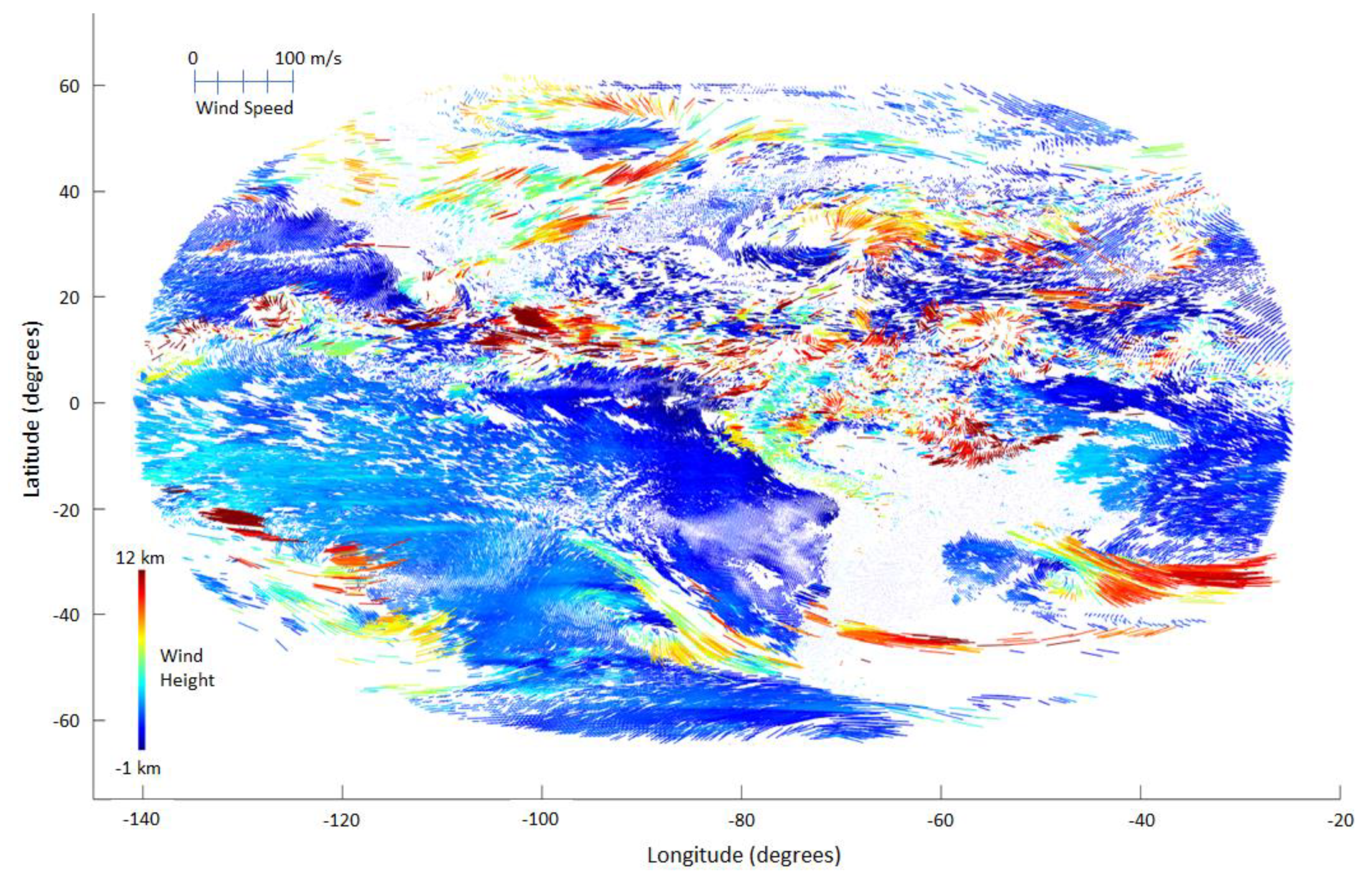
3.1. GEO-GEO Multi-Platform Winds
3.2. LEO-GEO Multi-Platform Winds
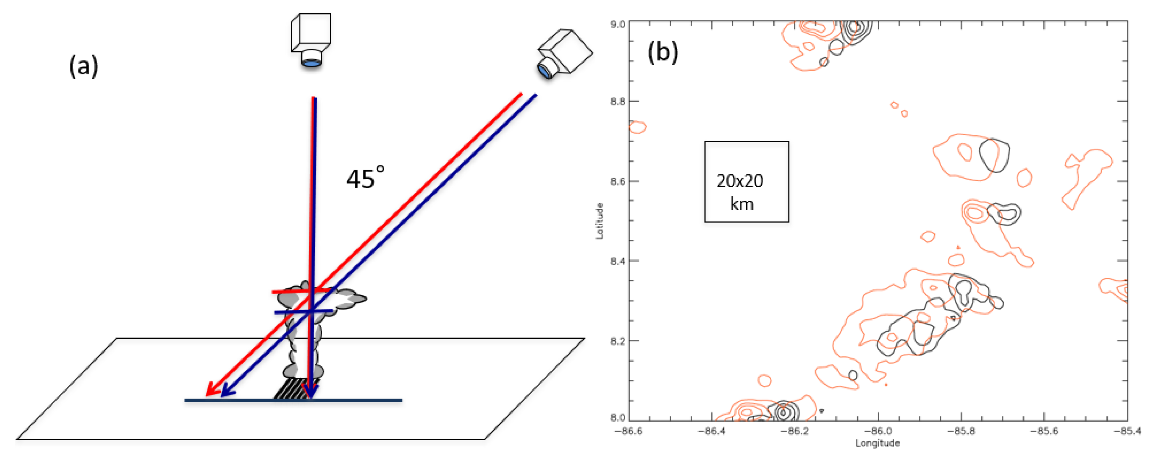
3.2.1. 3D-Wind Algorithm
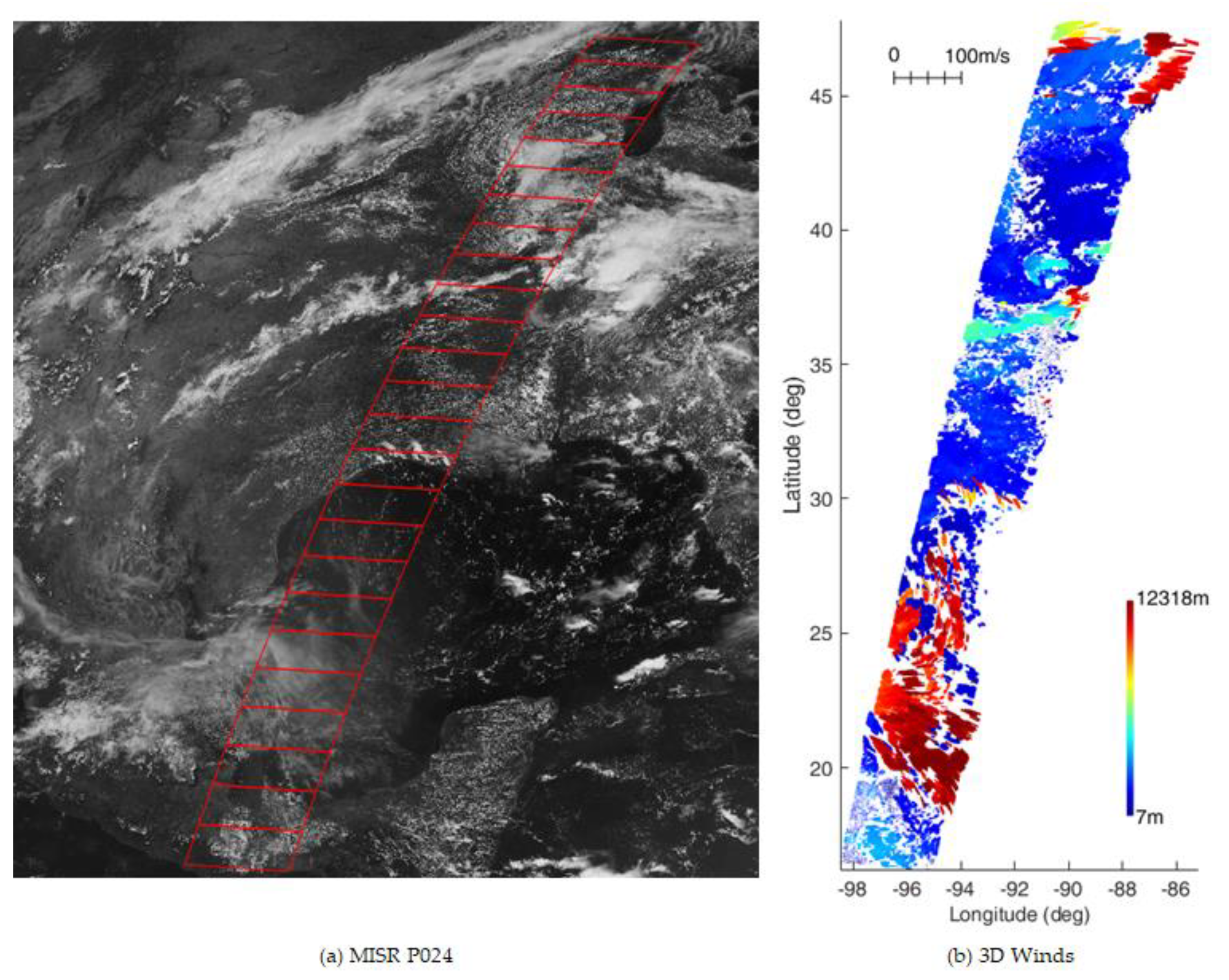
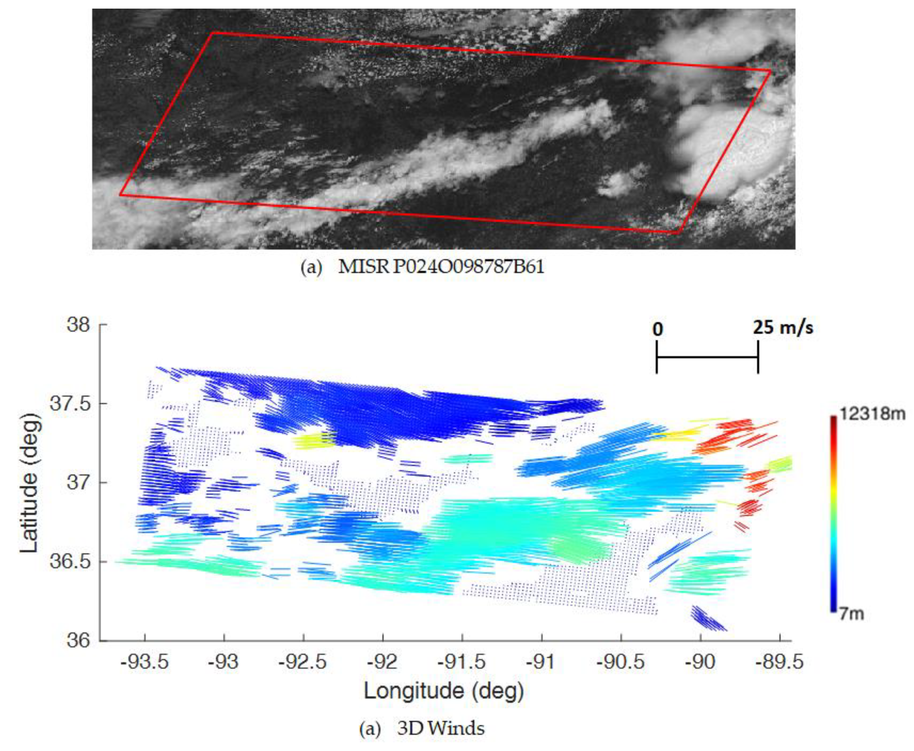
3.2.2. Results and Validation
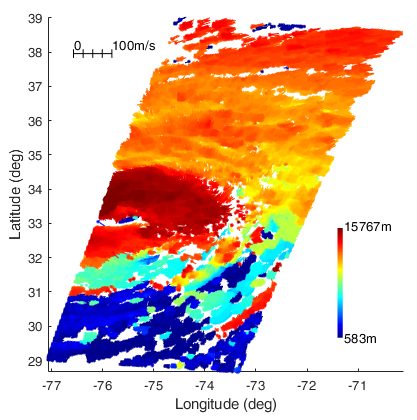
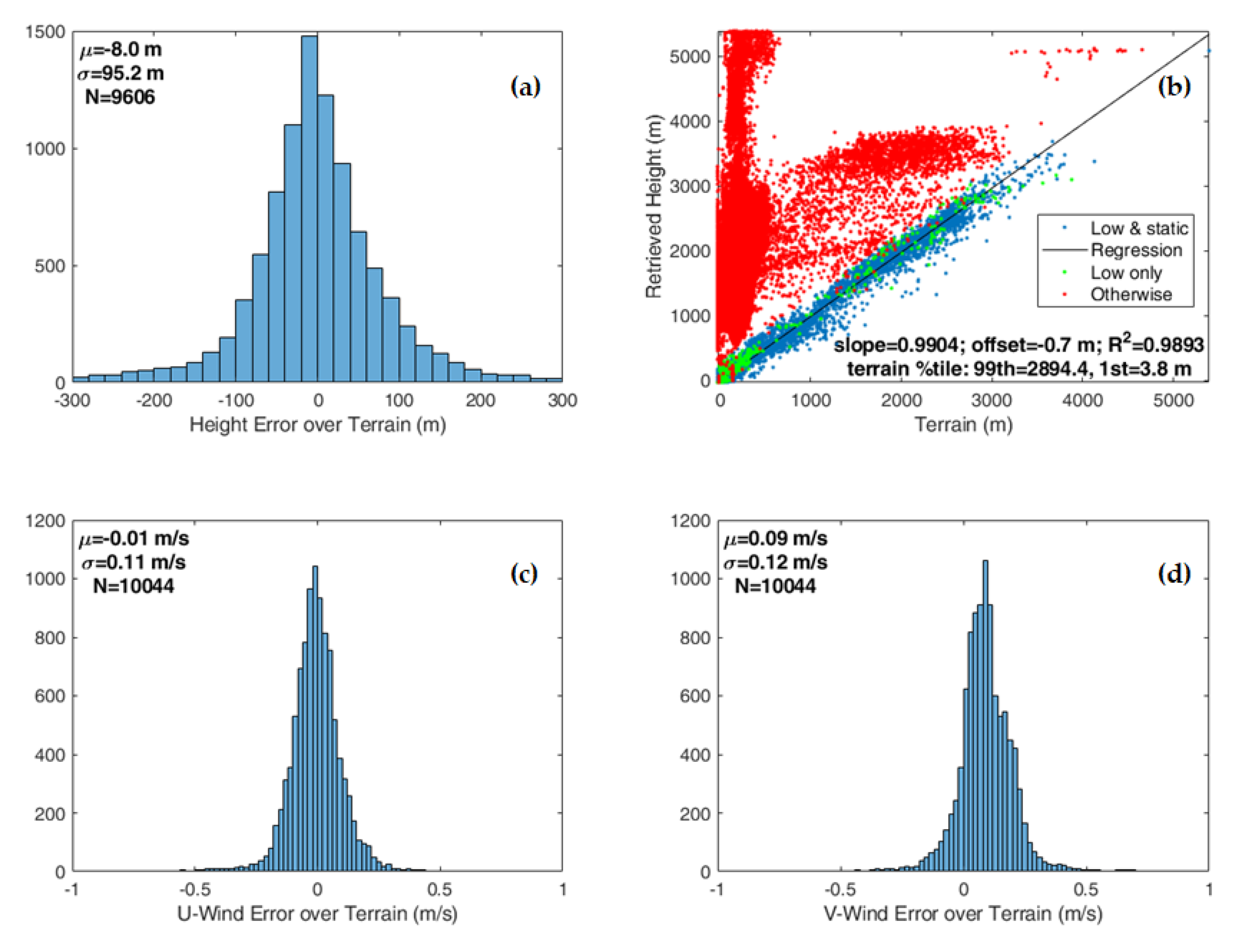
Clear-Sky Retrievals over Terrain
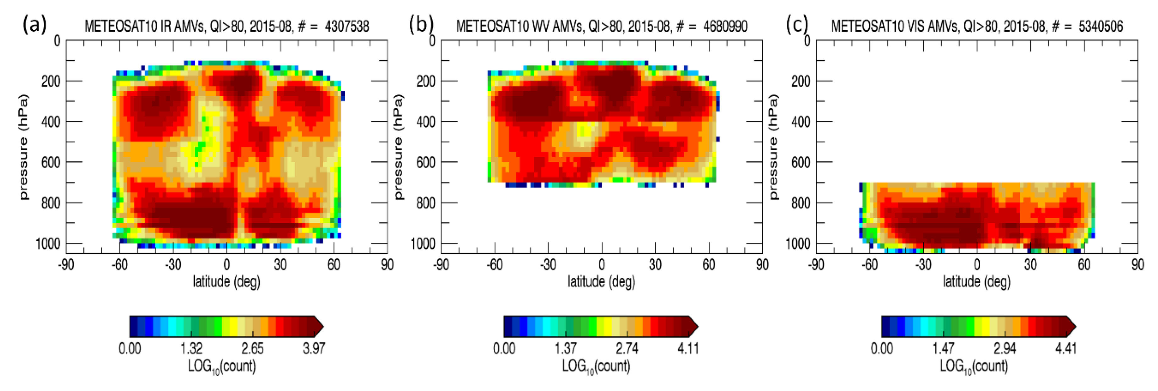
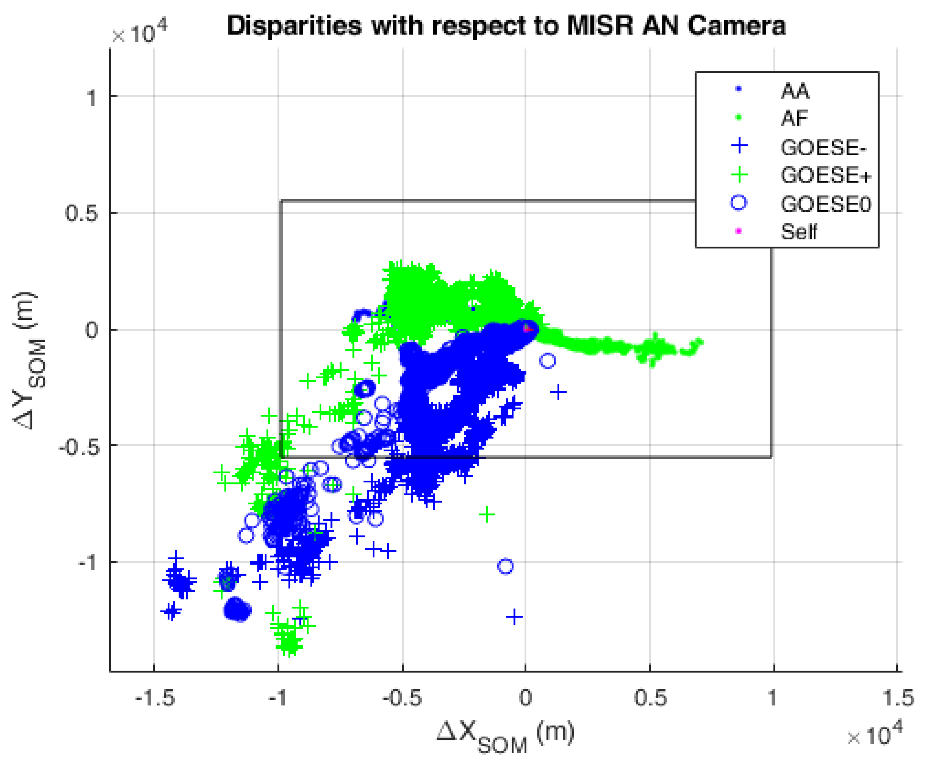
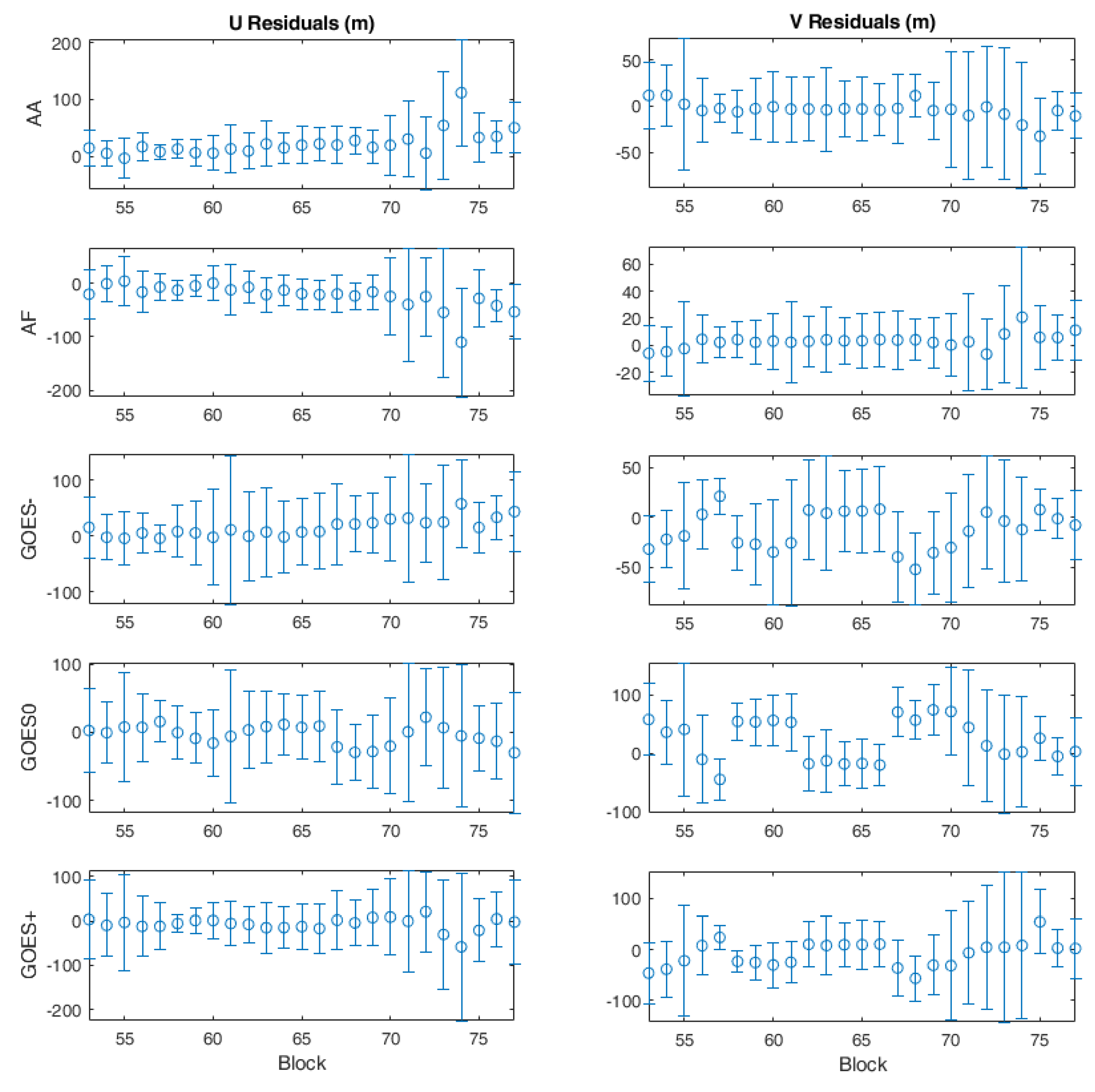
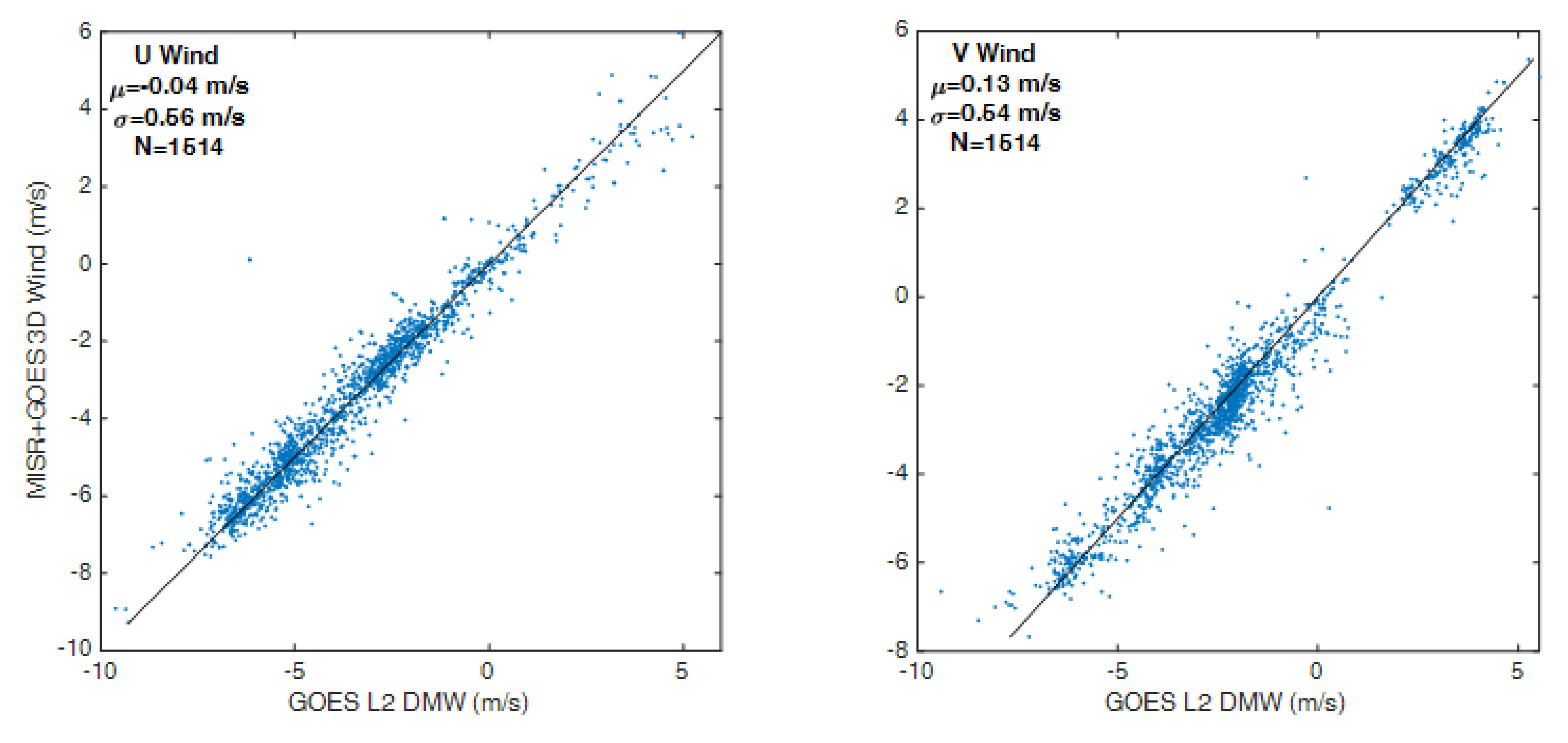
Comparisons with GOES Level-2 Derived Motion Winds
Comparisons with MISR Winds
MISR with GOES MESO Scenes
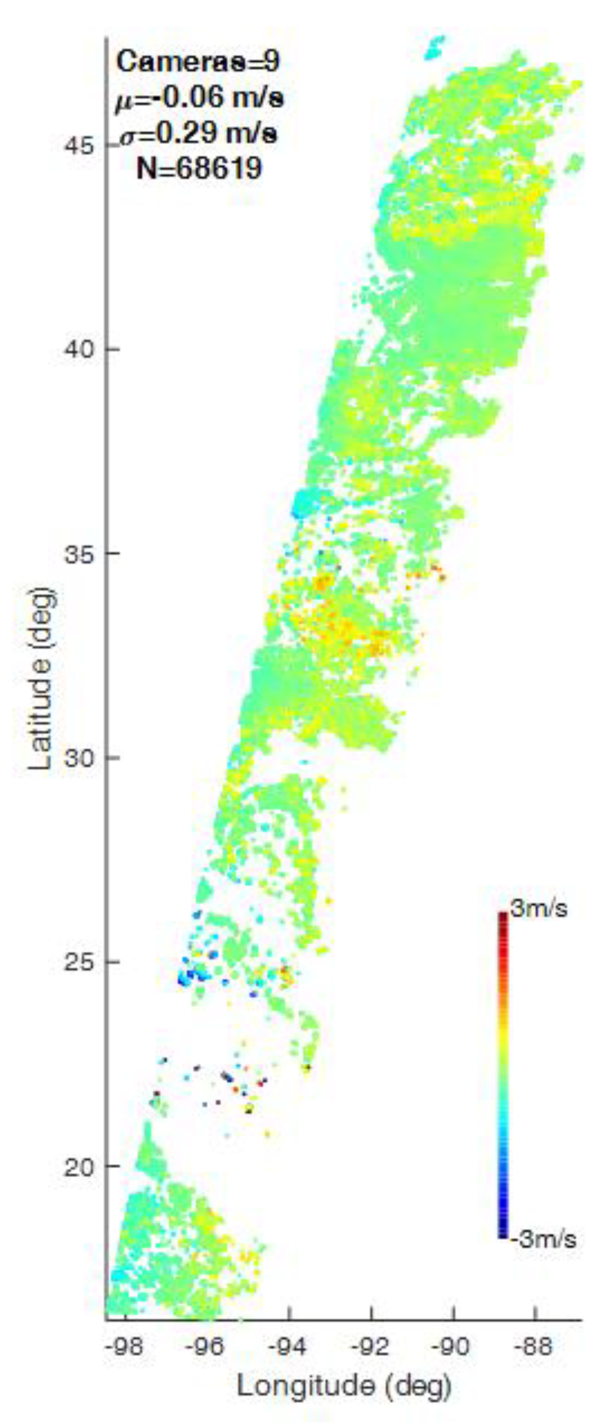
MISR B, C and D Cameras
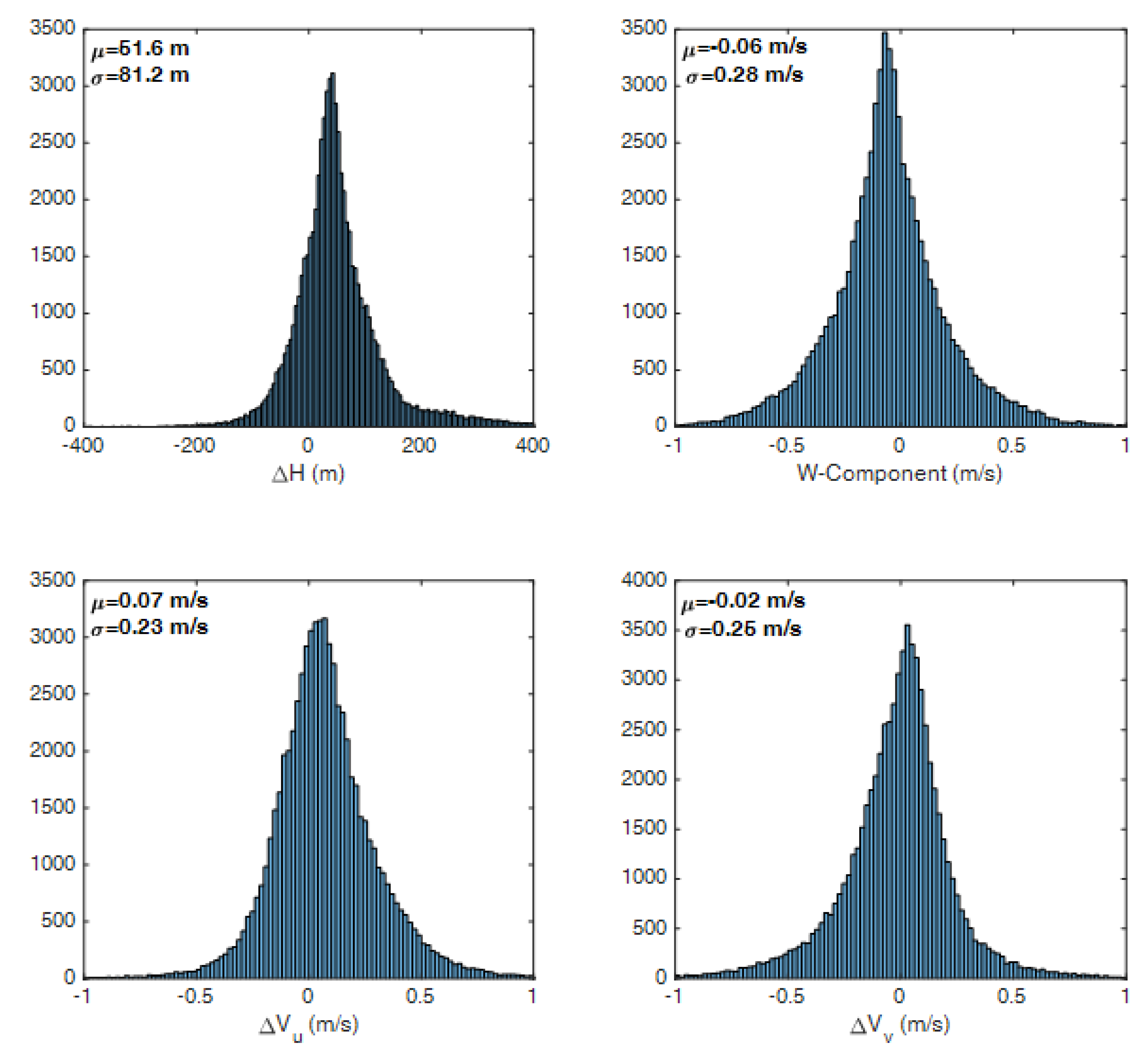
W-Component Retrievals
Summary of Validations and Comparisons
4. Discussions
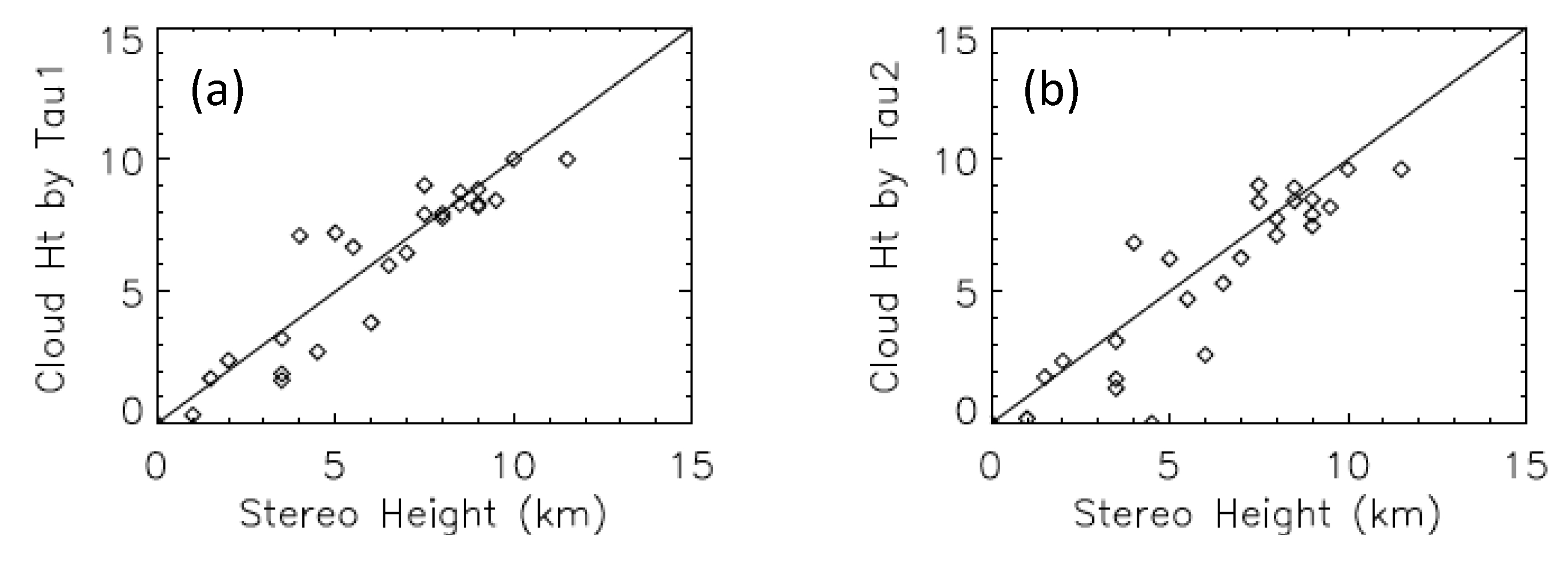
4.1. Stereo Height vs. IR Height
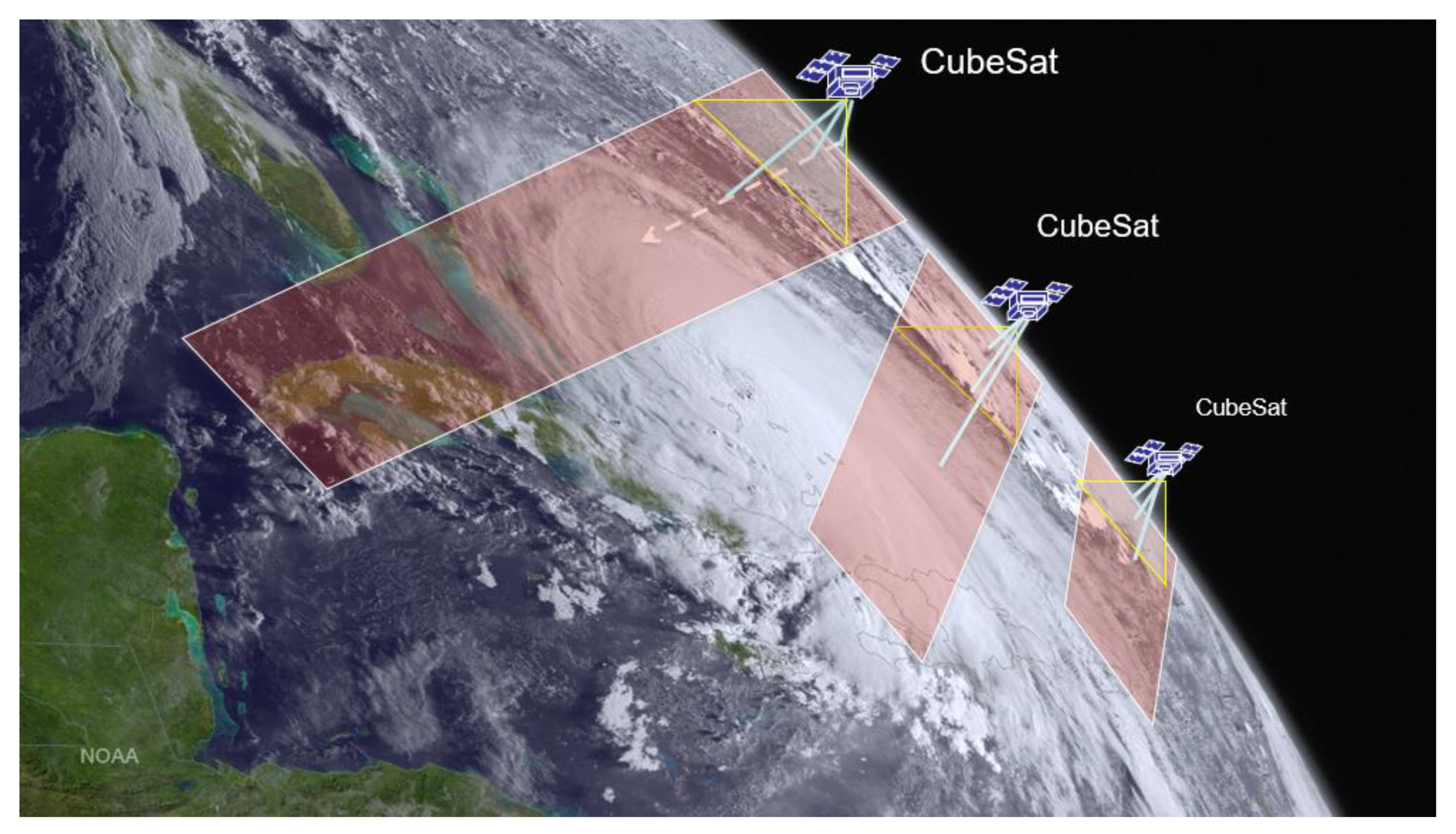
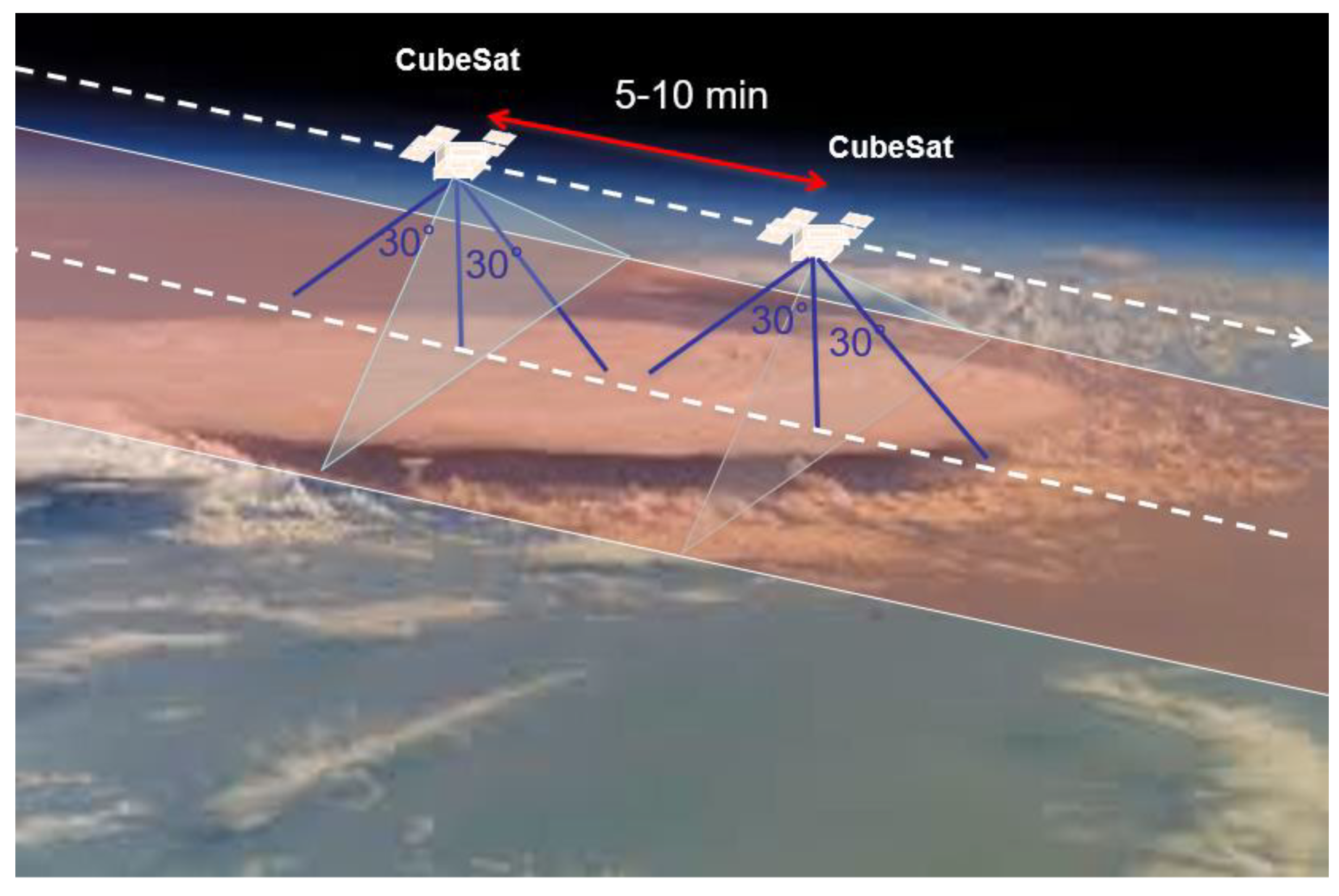
4.2. Future Global AMVs with CubeSat Constellations
4.3. Compact Midwave Imaging System (CMIS)
5. Conclusions
Supplementary Materials
Author Contributions
Funding
Acknowledgments
Conflicts of Interest
Appendix A. MISR-GOES 3D-Wind Algorithm Math Model
A.1. Formulation of the Problem.

A.2. Solution to the Static Problem.
A.3. Solution to the Dynamic Problem.
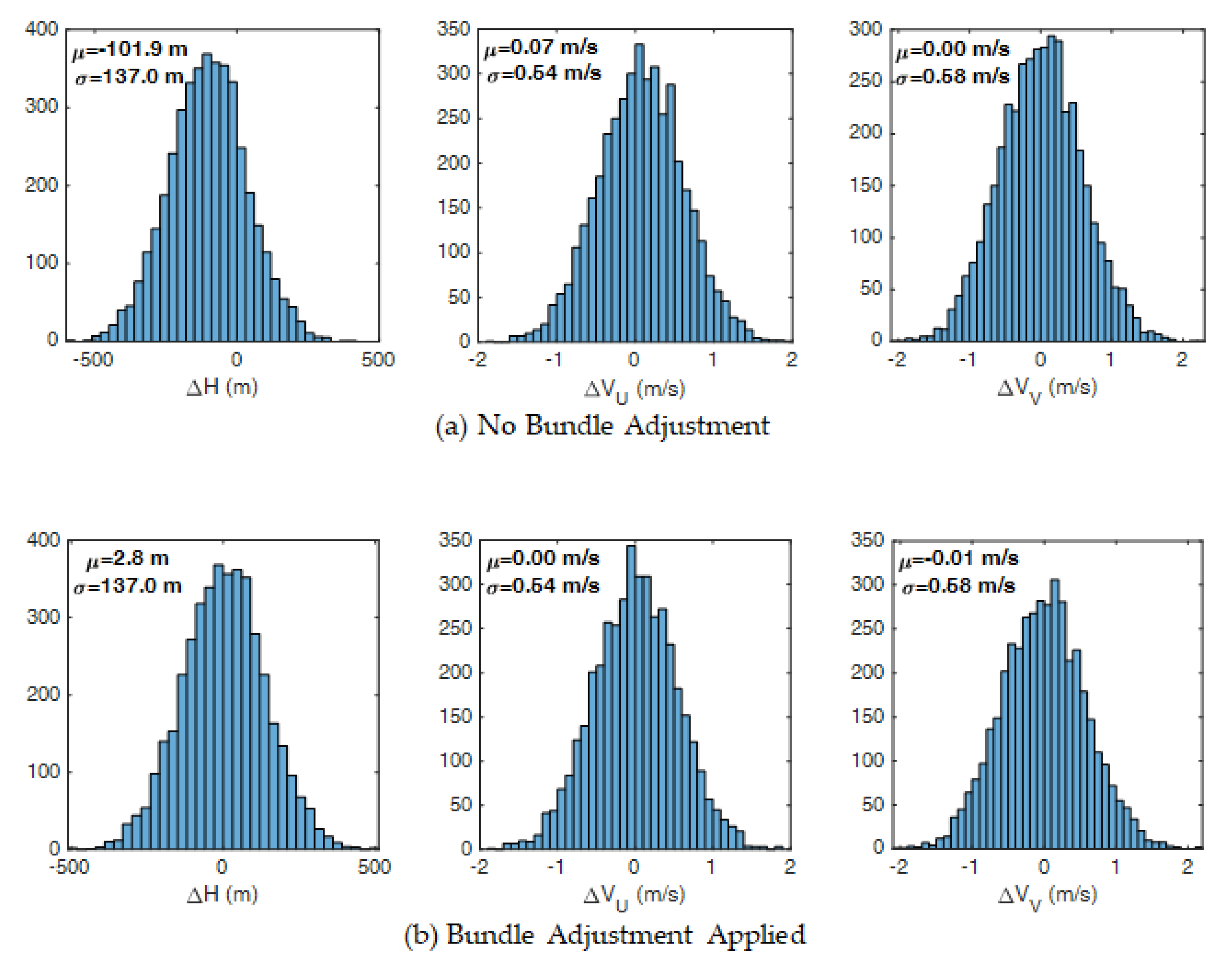
A.4. Bundle Adjustment.
References
- Kelly, G.; Thépaut, J.-N.; Buizza, R.; Cardinali, C. The value of observations. I: Data denial experiments for the Atlantic and the Pacific. Q. J. R. Meteorol. Soc. 2007, 133, 1803–1815. [Google Scholar] [CrossRef]
- Gelaro, R.; Langland, R.H.; Pellerin, S.; Todling, R. The THORPEX Observation Impact Intercomparison Experiment. Mon. Weather Rev. 2010, 138, 4009–4025. [Google Scholar] [CrossRef]
- Gelaro, R.; Zhu, Y. Examination of observation impacts derived from observing system experiments (OSEs) and adjoint models. Tellus A Dyn. Meteorol. Oceanogr. 2016, 61, 179–193. [Google Scholar] [CrossRef]
- Menzel, W.P.; Frey, R.A.; Zhang, H.; Wylie, D.P.; Moeller, C.C.; Holz, R.E.; Maddux, B.; Baum, B.A.; Strabala, K.I.; Gumley, L.E. MODIS Global Cloud-Top Pressure and Amount Estimation: Algorithm Description and Results. J. Appl. Meteorol. Clim. 2008, 47, 1175–1198. [Google Scholar] [CrossRef]
- Holz, R.E.; Ackerman, S.A.; Nagle, F.W.; Frey, R.; Dutcher, S.; Kuehn, R.E.; Vaughan, M.A.; Baum, B. Global Moderate Resolution Imaging Spectroradiometer (MODIS) cloud detection and height evaluation using CALIOP. J. Geophys. Res. Atmos. 2008, 113. [Google Scholar] [CrossRef]
- Berthier, S.; Chazette, P.; Pelon, J.; Baum, B. Comparison of cloud statistics from spaceborne lidar systems. Atmos. Chem. Phys. 2008, 8, 6965–6977. [Google Scholar] [CrossRef]
- Garay, M.J.; de Szoeke, S.P.; Moroney, C.M. Comparison of marine stratocumulus cloud top heights in the southeastern Pacific retrieved from satellites with coincident ship-based observations. J. Geophys. Res. 2008, 113. [Google Scholar] [CrossRef]
- Schmetz, J.; Nuret, M. Automatic Tracking of High-Level Clouds in Meteosat Infrared Images with a Radiance Windowing Technique. ESA J. 1987, 11, 275–286. [Google Scholar]
- Nieman, S.J.; Schmetz, J.; Menzel, W.P. A Comparison of Several Techniques to Assign Heights to Cloud Tracers. J. Appl. Meteorol. 1993, 32, 1559–1568. [Google Scholar] [CrossRef]
- Menzel, W.P.; Smith, W.L.; Stewart, T.R. Improved Cloud Motion Wind Vector and Altitude Assignment Using VAS. J. Clim. Appl. Meteorol. 1983, 22, 377–384. [Google Scholar] [CrossRef]
- Frey, R.A.; Baum, B.A.; Menzel, W.P.; Ackerman, S.A.; Moeller, C.C.; Spinhirne, J.D. A comparison of cloud top heights computed from airborne lidar and MAS radiance data using CO2 slicing. J. Geophys. Res. Atmos. 1999, 104, 24547–24555. [Google Scholar] [CrossRef]
- Szejwach, G. Determination of Semi-Transparent Cirrus Cloud Temperature from Infrared Radiances: Application to METEOSAT. J. Appl. Meteorol. 1982, 21, 384–393. [Google Scholar] [CrossRef]
- Schmetz, J.; Holmlund, K.; Hoffman, J.; Strauss, B.; Mason, B.; Gaertner, V.; Koch, A.; Berg, L.V.D. Operational Cloud-Motion Winds from Meteosat Infrared Images. J. Appl. Meteorol. 1993, 32, 1206–1225. [Google Scholar] [CrossRef]
- Borde, R.; Oyama, R. A Direct Link Between Feature Tracking and Height Assignment of Operational Atmospheric Motion Vectors. In Proceedings of the 9th International Winds Workshop, Annapolis, MD, USA, 14–18 April 2008. [Google Scholar]
- Borde, R.; Smet, A.D.; Arriaga, A. Height assignment of atmospheric motion vectors with Meteosat 8. In Proceedings of the Remote Sensing, Maspalomas, Spain, 30 November 2004; p. 9. [Google Scholar] [CrossRef]
- Zhang, H.; Menzel, W.P. Improvement in thin cirrus retrievals using an emissivity-adjusted CO2 slicing algorithm. J. Geophys. Res. Atmos. 2002, 107. [Google Scholar] [CrossRef]
- Velden, C.S.; Bedka, K.M. Identifying the Uncertainty in Determining Satellite-Derived Atmospheric Motion Vector Height Attribution. J. Appl. Meteorol. Clim. 2009, 48, 450–463. [Google Scholar] [CrossRef]
- Lean, K.; Bormann, N.; Salonen, K. Assessment of new AMV data in the ECMWF system: First year report. EUMETSAT/ECMWF Fellowship Programme Research Report No. 43. 2017. Available online: https://www.ecmwf.int/sites/default/files/elibrary/2017/16984-assessment-new-amv-data-ecmwf-system-first-year-report.pdf (accessed on 22 November 2018).
- Whitehead, V.S.; Browne, I.D.; Garcia, J.G. Cloud height contouring from Apollo 6 photography. Bull. Am. Meteorol. Soc. 1969, 50, 522–529. [Google Scholar] [CrossRef]
- Minzner, R.A.; Shenk, W.E.; Teagle, R.D.; Steranka, J. Stereographic cloud heights from imagery of SMS/GOES satellites. Geophys. Res. Lett. 1978, 5, 21–24. [Google Scholar] [CrossRef]
- Hasler, A.F. Stereographic Observations from Geosynchronous Satellites: An Important New Tool for the Atmospheric Sciences. Bull. Am. Meteorol. Soc. 1981, 62, 194–212. [Google Scholar] [CrossRef]
- Mack, R.; Hasler, A.F.; Rodgers, E.B. Stereoscopic observations of hurricanes and tornadic thunderstorms from geosynchronous satellites. Adv. Space Res. 1983, 2, 143–151. [Google Scholar] [CrossRef]
- Takashima, T.; Takayama, Y.; Matsuura, K.; Naito, K. Cloud Height Determination by Satellite Stereography. Pap. Meteorol. Geophys. 1982, 33, 65–78. [Google Scholar] [CrossRef]
- Fujita, T.T.; Dodge, J.C. Applications of stereoscopic height computations from dual geosynchronous satellite data/joint NASA-Japan stereo project. Adv. Space Res. 1983, 2, 153–160. [Google Scholar] [CrossRef]
- Lancaster, R.S.; Spinhirne, J.D.; Manizade, K.F. Combined Infrared Stereo and Laser Ranging Cloud Measurements from Shuttle Mission STS-85. J. Atmos. Ocean. Technol. 2003, 20, 67–78. [Google Scholar] [CrossRef]
- Horváth, Á.; Davies, R. Simultaneous retrieval of cloud motion and height from polar-orbiter multiangle measurements. Geophys. Res. Lett. 2001, 28, 2915–2918. [Google Scholar] [CrossRef]
- Zong, J.; Davies, R.; Muller, J.P.; Diner, D.J. Photogrammetric retrieval of cloud advection and top height from the multi-angle imaging spectroradiometer (MISR). Photogramm. Eng. Remote Sens. 2002, 68, 821–829. [Google Scholar]
- Davies, R.; Horváth, Á.; Moroney, C.; Zhang, B.; Zhu, Y. Cloud motion vectors from MISR using sub-pixel enhancements. Remote Sens. Environ. 2007, 107, 194–199. [Google Scholar] [CrossRef]
- Diner, D.J.; Braswell, B.H.; Davies, R.; Gobron, N.; Hu, J.; Jin, Y.; Kahn, R.A.; Knyazikhin, Y.; Loeb, N.; Muller, J.-P.; et al. The value of multiangle measurements for retrieving structurally and radiatively consistent properties of clouds, aerosols, and surfaces. Remote Sens. Environ. 2005, 97, 495–518. [Google Scholar] [CrossRef]
- Mueller, K.J.; Wu, D.L.; Horváth, Á.; Jovanovic, V.M.; Muller, J.-P.; Girolamo, L.D.; Garay, M.J.; Diner, D.J.; Moroney, C.M.; Wanzong, S. Assessment of MISR Cloud Motion Vectors (CMVs) Relative to GOES and MODIS Atmospheric Motion Vectors (AMVs). J. Appl. Meteorol. Clim. 2017, 56, 555–572. [Google Scholar] [CrossRef]
- Key, J.R.; Santek, D.; Velden, C.S.; Bormann, N.; Thepaut, J.; Riishojgaard, L.P.; Yanqiu, Z.; Menzel, W.P. Cloud-drift and water vapor winds in the polar regions from MODISIR. IEEE Trans. Geosci. Remote Sens. 2003, 41, 482–492. [Google Scholar] [CrossRef]
- Dworak, R.; Key, J.R. Twenty Years of Polar Winds from AVHRR: Validation and Comparison with ERA-40. J. Appl. Meteorol. Clim. 2009, 48, 24–40. [Google Scholar] [CrossRef]
- Santek, D. The Impact of Satellite-Derived Polar Winds on Lower-Latitude Forecasts. Mon. Weather Rev. 2010, 138, 123–139. [Google Scholar] [CrossRef]
- Lazzara, M.A.; Coletti, A.; Diedrich, B.L. The possibilities of polar meteorology, environmental remote sensing, communications and space weather applications from Artificial Lagrange Orbit. Adv. Space Res. 2011, 48, 1880–1889. [Google Scholar] [CrossRef]
- Santek, D.; Nebuda, S.; Stettner, D. Feature-tracked winds from moisture fields derived from AIRS sounding retrievals. In Proceedings of the 12th International Winds Workshop, Copenhagen, Denmark, 15–20 June 2014; p. 7655. [Google Scholar]
- Hautecoeur, O.; Borde, R. Derivation of Wind Vectors from AVHRR/MetOp at EUMETSAT. J. Atmos. Ocean. Technol. 2017, 34, 1645–1659. [Google Scholar] [CrossRef]
- Madani, H.; Carr, J.L. Stereo Cloud Top Height Products for the GOES-R Era. In Proceedings of the NOAA Satellite Conference, Greenbelt, Maryland, 27 April–1 May 2015. [Google Scholar]
- Carr, J.L.; Gibbs, B.; Madani, H.; Allen, N. INR Performance of the GOES-13 Spacecraft Measured in Orbit. In Proceedings of the 31st Annual Rocky Mountain Guidance, Navigation and Control Conference, Breckenridge, CO, USA, 1–6 February 2008. [Google Scholar]
- Gall, D.; Virgilio, V.; Forkert, R.; Van Naarden, J.; Griffith, P. GOES-16 ABI On-Orbit INR Tuning and Performance. Adv. Astronautical Sci. 2018, 164, 821. Available online: http://www.univelt.com/linkedfiles/v164%20Contents.pdf (accessed on 22 November 2018).
- Madani, H.; Carr, J.L.; Heidinger, A.; Wanzong, S. Inter-Comparisons between Radiometric and Geometric Cloud Top Height Products. Am. Geophys. Union 2015. Available online: https://agu.confex.com/agu/fm15/mediafile/Handout/Paper76215/AGU_HouriaMadani_A33E_0220.pdf (accessed on 22 November 2018).
- Carr, J.L. Multi-Satellite 3D Winds. NOAA Emerging Technologies Workshop; 2017. Available online: https://nosc.noaa.gov/2017_NOAA_ETW/7_RFI_Session2/ (accessed on 22 November 2018).
- Goes-R Series Product Definition and Users’ Guide (PUG). 2018. Available online: https://www.goes-r.gov/users/docs/PUG-main-vol1.pdf (accessed on 22 November 2018).
- Muller, J.; Mandanayake, A.; Moroney, C.; Davies, R.; Diner, D.J.; Paradise, S. MISR stereoscopic image matchers: Techniques and results. IEEE Trans. Geosci. Remote Sens. 2002, 40, 1547–1559. [Google Scholar] [CrossRef]
- Mueller, K.; Moroney, C.; Jovanovic, V.; Garay, M.; Muller, J.; Girolamo, L.; Davies, R. (2013) MISR Level 2 cloud product algorithm theoretical basis. JPL Tech. Doc. 2013. Available online: https://eospso.nasa.gov/sites/default/files/atbd/MISR_L2_CLOUD_ATBD-1.pdf. (accessed on 22 November 2018).
- Lewis, J.P. Fast Normalized Cross-Correlation. Industrial Light and Magic. 1995. Available online: https://www.researchgate.net/publication/2378357_Fast_Normalized_Cross-Correlation (accessed on 22 November 2018).
- Carr, J.L.; Moigne, J.; Netanyahu, N.; Eastman, R. Image Registration for Remote Sens; Cambridge University Press: Cambridge, UK, 2010. [Google Scholar]
- Kalluri, S.; Alcala, C.; Carr, J.; Griffith, P.; Lebair, W.; Lindsey, D.; Race, R.; Wu, X.; Zierk, S. From Photons to Pixels: Processing Data from the Advanced Baseline Imager. Remote Sens. 2018, 10, 177. [Google Scholar] [CrossRef]
- Jovanovic, V.; Moroney, C.; Nelson, D. Multi-angle geometric processing for globally geo-located and co-registered MISR image data. Remote Sens. Environ. 2007, 107, 22–32. [Google Scholar] [CrossRef]
- Horváth, Á. Improvements to MISR stereo motion vectors. J. Geophys. Res. Atmos. 2013, 118, 5600–5620. [Google Scholar] [CrossRef]
- Hastings, D.; Dunbar, P. Global Land One-kilometer Base Elevation (GLOBE) Digital Elevation Model, Documentation. NGDC Key to Geophysical Records Documentation; 1999; Volume 1, p. 34. Available online: https://www.ngdc.noaa.gov/mgg/topo/report/globedocumentationmanual.pdf (accessed on 22 November 2018).
- Lemoine, F.; Kenyon, S.; Factor, J.; Trimmer, R.; Pavlis, N.; Chinn, D.; Cox, C.; Klosko, S.; Luthcke, S.; Torrence, M.; et al. The Development of the Joint NASA GSFC and the National Imagery and Mapping Agency (NIMA) Geopotential Model EGM96. NASA/TP-1998-206861; 1998. Available online: https://science.gsfc.nasa.gov/sed/content/uploadFiles/publication_files/EGM96_NASA-TP-1998-206861.pdf (accessed on 22 November 2018).
- Moroney, C.; Horvath, A.; Davies, R. Use of stereo-matching to coregister multiangle data from MISR. IEEE Trans. Geosci. Remote Sens. 2002, 40, 1541–1546. [Google Scholar] [CrossRef]
- Lonitz, K.; Horváth, Á. Comparison of MISR and Meteosat-9 cloud-motion vectors. J. Geophys. Res. Atmos. 2011, 116. [Google Scholar] [CrossRef]
- Gelaro, R.; McCarty, W.; Suárez, M.J.; Todling, R.; Molod, A.; Takacs, L.; Randles, C.A.; Darmenov, A.; Bosilovich, M.G.; Reichle, R.; et al. The Modern-Era Retrospective Analysis for Research and Applications, Version 2 (MERRA-2). J. Clim. 2017, 30, 5419–5454. [Google Scholar] [CrossRef]
- Baker, N.; Pauley, P.; Langland, R.; Mueller, K.; Wu, D. An Assessment of the Impact of the Assimilation of NASA Terra MISR Atmospheric Motion Vectors on the NRL Global Atmospheric Prediction System. 2014. Available online: https://ams.confex.com/ams/94Annual/webprogram/Paper231106.html (accessed on 22 November 2018).
- Luo, J.Z.; Jeyaratnam, J.; Iwasaki, S.; Takahashi, H.; Anderson, R. Convective vertical velocity and cloud internal vertical structure: An A-Train perspective. Geophys. Res. Lett. 2014, 41, 723–729. [Google Scholar] [CrossRef]
- Marchand, R.; Ackerman, T.; Smyth, M.; Rossow, W.B. A review of cloud top height and optical depth histograms from MISR, ISCCP, and MODIS. J. Geophys. Res. 2010, 115, D16206. [Google Scholar] [CrossRef]
- Liu, Q.; Weng, F. Advanced Doubling–Adding Method for Radiative Transfer in Planetary Atmospheres. J. Atmos. Sci. 2006, 63, 3459–3465. [Google Scholar] [CrossRef]
- Rienecker, M.M.; Suarez, M.J.; Gelaro, R.; Todling, R.; Julio, B.; Liu, E.; Bosilovich, M.G.; Schubert, S.D.; Takacs, L.; Kim, G.-K.; et al. MERRA: NASA’s Modern-Era Retrospective Analysis for Research and Applications. J. Clim. 2011, 24, 3624–3648. [Google Scholar] [CrossRef]
- Gong, J.; Wu, D.L.; Limpasuvan, V. Meridionally tilted ice cloud structures in the tropical upper troposphere as seen by CloudSat. Atmos. Chem. Phys. 2015, 15, 6271–6281. [Google Scholar] [CrossRef]
- Várnai, T.; Davies, R. Effects of Cloud Heterogeneities on Shortwave Radiation: Comparison of Cloud-Top Variability and Internal Heterogeneity. J. Atmos. Sci. 1999, 56, 4206–4224. [Google Scholar] [CrossRef]
- Muller, J.-P. WINDS: Demonstrating How to Map the Earth’s Winds 24 h Per Day—A Proposal to EE-8. Mullard Space Science Laboratory, University College London, London, UK. 2010. Available online: https://cdn.knmi.nl/system/data_center_publications/files/000/068/580/original/winds_proposal_for_ee8_issue_1.pdf?1495621279 (accessed on 22 November 2018).
- Wood, R.; Wu, D.L.; Diner, D.J.; Garay, M.J.; Jovanovic, V. Spaceborne Atmospheric Boundary Layer Explorer (SABLE)—Earth Venture-2 Mission Proposal. University of Washington, Washington, USA. 2011. Available online: http://cimss.ssec.wisc.edu/iwwg/iww11/talks/Session6_Diner.pdf (accessed on 22 November 2018).
- Muller, J.-P.; Walton, D.; Fisher, D.; Cole, R. SMVs (Stereo Motion Vectors) from ASTR2-AATSR and MISRlite (Multi-Angle Infrared Stereo Radiometer) Constellation. In Proceedings of the 10th International Winds Workshop, Tokyo, Japan, 22–26 February 2010. [Google Scholar]
- Rennó, N.O.; Williams, E.; Rosenfeld, D.; Fischer, D.G.; Fischer, J.; Kremic, T.; Agrawal, A.; Andreae, M.O.; Bierbaum, R.; Blakeslee, R.; et al. CHASER: An Innovative Satellite Mission Concept to Measure the Effects of Aerosols on Clouds and Climate. Bull. Am. Meteorol. Soc. 2013, 94, 685–694. [Google Scholar] [CrossRef]
- Goldberg, A.C.; Kelly, M.A.; Boldt, J.; Wu, D.L.; Heidinger, A.; Wilson, J.P.; Ryan, K.J.; Morgan, M.F.; Yee, J.H.; Greenberg, J.M.; et al. Compact midwave imaging system (CMIS) for weather satellite applications. In Proceedings of the SPIE Defense + Security, Baltimore, MD, USA, 14–18 April 2018; p. 16. [Google Scholar]
- Hirschmuller, H. Stereo Processing by Semiglobal Matching and Mutual Information. IEEE Trans. Pattern Analysis Mach. Intell. 2008, 30, 328–341. [Google Scholar] [CrossRef] [PubMed]
- Petrick, D.; Geist, A.; Albaijes, D.; Davis, M.; Sparacino, P.; Crum, G.; Ripley, R.; Boblitt, J.; Flatley, T. SpaceCube v2.0 space flight hybrid reconfigurable data processing system. In Proceedings of the 2014 IEEE Aerospace Conference, Big Sky, MT, USA, 1–8 March 2014; pp. 1–20. [Google Scholar]
- Szeliski, R. Computer Vision; Springer: London, UK, 2011. [Google Scholar]


- (a)
- Retrieved ellipsoid heights compared to clear-sky over terrain heights. In each case, parameters are given for the regression of retrieved height versus terrain height as well as the sample size (Nterrain) and 1%-to-99% range of terrain heights. Sample means (μ) and standard deviations (σ) of the differences between the retrieval and the terrain heights (ΔH) indicate the accuracy of the height retrievals.
| Regression | Terrain | Errors | |||||||
|---|---|---|---|---|---|---|---|---|---|
| MISR Path+Orbit | GOES | Nterrain | Slope | Offset (m) | R2 | 1% (m) | 99% (m) | μ(ΔH) (m) | σ(ΔH) (m) |
| P008O098097 | 16 | water | - | - | water | - | - | - | - |
| P024O098098 | 16 | 30,983 | 0.9984 | 11.7 | 0.9864 | –2.7 | 2676.8 | 11.1 | 68.3 |
| P040O098099 | 16 | 26,716 | 0.9817 | 51.0 | 0.9467 | –81.3 | 2367.9 | 35.7 | 126.9 |
| P008O098796 | 16 | water | - | - | water | - | - | - | - |
| P008O098796 | 17 | water | - | - | water | - | - | - | - |
| P024O098797 | 16 | 9606 | 0.9904 | –0.7 | 0.9893 | 3.8 | 2894.4 | –8.0 | 95.2 |
| P024O098797 | 17 | 4695 | 1.0725 | 2.2 | 0.9031 | –0.2 | 409.5 | 9.2 | 45.5 |
| P040O098798 | 16 | 30,138 | 0.9273 | 165.4 | 0.9230 | 278.1 | 2566.7 | 60.1 | 128.6 |
| P040O098798 | 17 | 55,557 | 0.9710 | 76.8 | 0.9513 | 16.5 | 2678.5 | 34.9 | 123.6 |
- (b)
- Retrieved AMVs for clear-sky over terrain. In each case, the sample mean (μ) and standard deviation (σ) statistics for the AMV components of clear-sky terrain retrievals are presented. Since these are presumably stationary objects, such statistics are indicative of the accuracy of the retrieved velocities.
| MISR Path+Orbit | GOES | Nterrain | μ(VU) (m/s) | σ(VU) (m/s) | μ(VV) (m/s) | σ(VV) (m/s) |
|---|---|---|---|---|---|---|
| P008O098097 | 16 | water | - | - | - | - |
| P024O098098 | 16 | 33,414 | −0.03 | 0.12 | −0.00 | 0.18 |
| P040O098099 | 16 | 29,256 | −0.08 | 0.14 | 0.04 | 0.15 |
| P008O098796 | 16 | water | − | − | − | − |
| P008O098796 | 17 | water | − | − | − | − |
| P024O098797 | 16 | 10,044 | −0.01 | 0.11 | 0.09 | 0.12 |
| P024O098797 | 17 | 9412 | −0.26 | 0.40 | −0.04 | 0.13 |
| P040O098798 | 16 | 61,125 | −0.06 | 0.13 | −0.19 | 0.27 |
| P040O098798 | 17 | 61,770 | −0.14 | 0.10 | 0.12 | 0.10 |
| MISR Path+Orbit | GOES | N3D | NPaired | μ(ΔVU) (m/s) | σ(ΔVU) (m/s) | μ(ΔVV) (m/s) | σ(ΔVV) (m/s) |
|---|---|---|---|---|---|---|---|
| P008O098097 | 16 | 85,461 | 715 | 0.22 | 0.81 | 0.30 | 0.87 |
| P024O098098 | 16 | 122,339 | 1514 | −0.04 | 0.56 | 0.13 | 0.54 |
| P040O098099 | 16 | 59,731 | 90 | −0.02 | 1.04 | 0.47 | 1.06 |
| P008O098796 | 16 | 76,791 | 2391 | −0.04 | 0.55 | 0.07 | 0.54 |
| P008O098796 | 17 | 76,869 | 2397 | −0.17 | 0.59 | 0.22 | 0.57 |
| P024O098797 | 16 | 111,894 | 941 | 0.01 | 0.48 | 0.23 | 0.56 |
| P024O098797 | 17 | 112,501 | 941 | −0.17 | 0.48 | 0.22 | 0.59 |
| P040O098798 | 16 | 71,409 | 31 | 0.27 | 1.67 | −0.32 | 0.88 |
| P040O098798 | 17 | 72,025 | 30 | 0.12 | 1.72 | −0.13 | 0.75 |
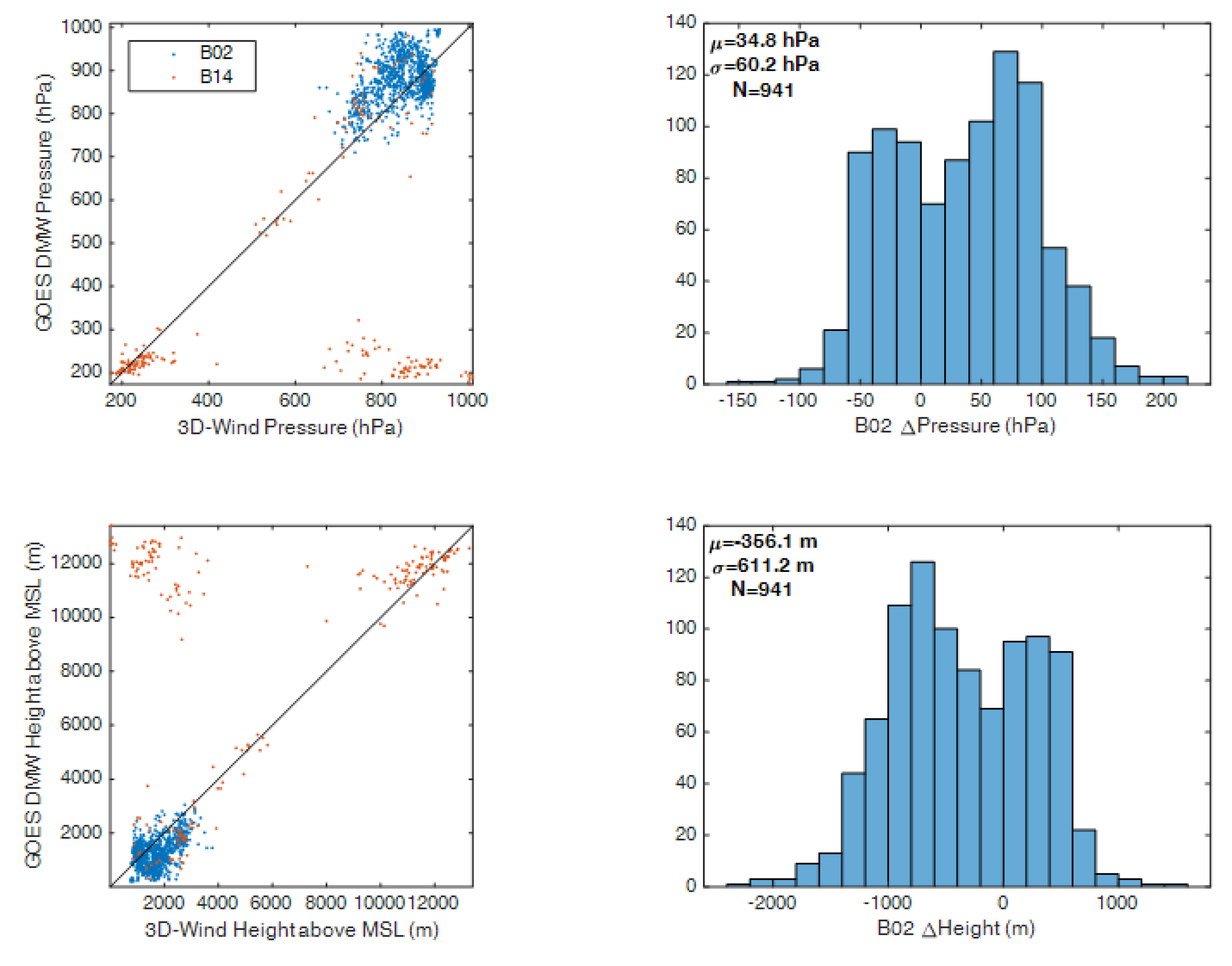
| MISR Path+Orbit | GOES | NPaired | μ(ΔP) (hPa) | σ(ΔP) (hPa) | μ(ΔH) (m) | σ(ΔH) (m) |
|---|---|---|---|---|---|---|
| P008O098097 | 16 | 715 | 43.1 | 70.7 | -419.8 | 732.1 |
| P024O098098 | 16 | 1514 | 93.5 | 38.6 | −936.8 | 392.2 |
| P040O098099 | 16 | 90 | 116.0 | 75.8 | −1332.3 | 863.4 |
| P008O098796 | 16 | 2391 | 65.6 | 60.3 | −628.8 | 600.3 |
| P008O098796 | 17 | 2397 | 67.1 | 59.9 | −644.1 | 597.3 |
| P024O098797 | 16 | 941 | 34.8 | 60.2 | −356.1 | 611.2 |
| P024O098797 | 17 | 941 | 34.2 | 60.0 | −349.5 | 608.5 |
| P040O098798 | 16 | 31 | 16.9 | 28.3 | −145.4 | 351.8 |
| P040O098798 | 17 | 30 | 19.8 | 27.7 | −172.9 | 345.2 |
| MISR Path+Orbit | GOES | μ(ΔH) (km) | σ(ΔH) (km) | μ(ΔVU) (m/s) | σ(ΔVU) (m/s) | μ(ΔVV) (m/s) | σ(ΔVV) (m/s) |
|---|---|---|---|---|---|---|---|
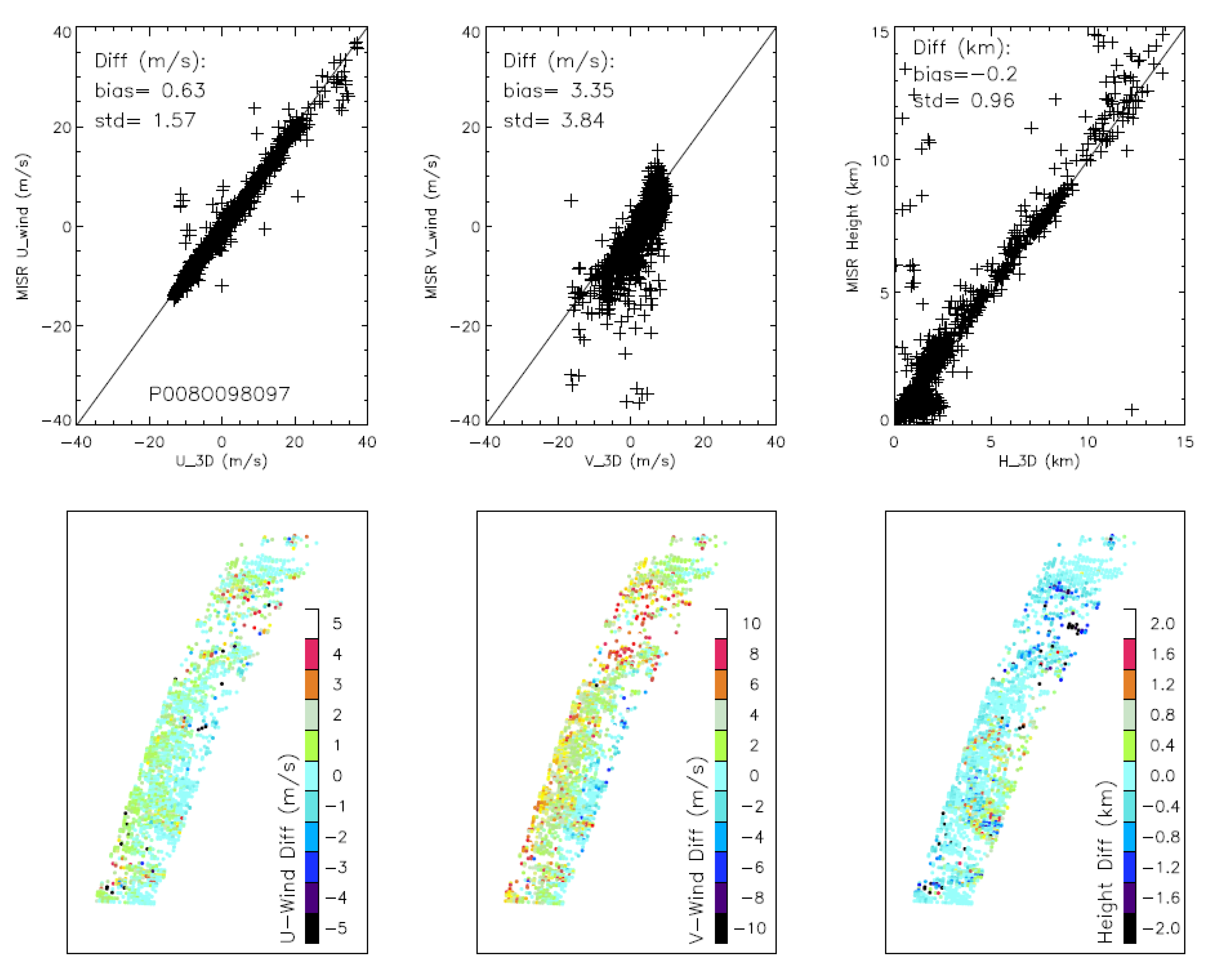
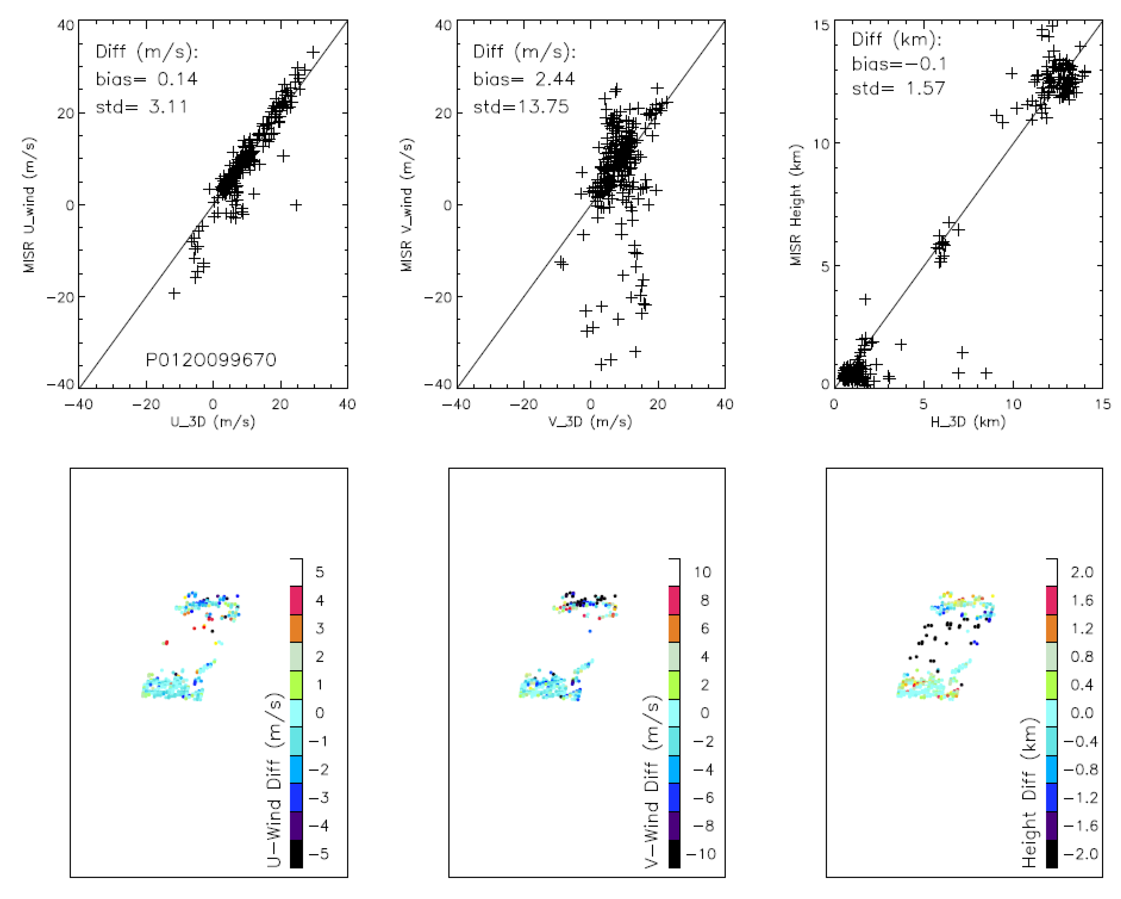
| P008O098097 | 16 | −0.2 | 0.96 | 0.63 | 1.57 | 3.35 | 3.84 |
| P024O098098 | 16 | 0.2 | 0.63 | −0.21 | 1.30 | −0.52 | 2.52 |
| P040O098099 | 16 | 0.1 | 0.72 | 0.30 | 1.31 | 0.33 | 3.98 |
| P008O098796 | 16 | 0.0 | 0.77 | 0.26 | 1.35 | 0.94 | 3.30 |
| P008O098796 | 17 | 0.0 | 0.77 | 0.34 | 1.33 | 0.75 | 3.30 |
| P024O098797 | 16 | 0.1 | 0.58 | 0.08 | 1.15 | 0.14 | 3.43 |
| P024O098797 | 17 | 0.1 | 0.63 | 0.15 | 1.15 | 0.10 | 3.40 |
| P040O098798 | 16 | 0.2 | 0.74 | 0.07 | 0.88 | 0.27 | 1.62 |
| P040O098798 | 17 | 0.1 | 0.70 | −0.01 | 0.70 | 0.57 | 1.61 |
| MISR Path+Orbit | Cameras | N3D | Nterrain for ΔH | μ(ΔH) (m) | σ(ΔH) (m) | Nterrain for V | μ(VU) (m/s) | σ(VU) (m/s) | μ(VV) (m/s) | σ(VV) (m/s) |
|---|---|---|---|---|---|---|---|---|---|---|
| P024O098797 | A | 111,894 | 9606 | −8.0 | 95.2 | 10,044 | −0.01 | 0.11 | 0.09 | 0.12 |
| P024O098797 | AB | 105,131 | 8952 | 13.4 | 82.9 | 9435 | 0.08 | 0.12 | 0.07 | 0.12 |
| P024O098797 | ABC | 90,230 | 7643 | 7.6 | 77.0 | 8152 | 0.08 | 0.12 | 0.07 | 0.12 |
| P024O098797 | ABCD | 69,249 | 5116 | 38.7 | 67.2 | 5310 | 0.06 | 0.12 | 0.01 | 0.09 |
| P040O098798 | A | 71,409 | 30,138 | 60.1 | 128.6 | 61,125 | −0.06 | 0.13 | −0.19 | 0.27 |
| P040O098798 | AB | 68,956 | 27,130 | 24.5 | 116.1 | 58,498 | −0.05 | 0.14 | −0.19 | 0.29 |
| P040O098798 | ABC | 61,826 | 25,324 | 22.9 | 106.8 | 53,395 | −0.07 | 0.15 | −0.19 | 0.29 |
| P040O098798 | ABCD | 50,403 | 18,720 | 40.6 | 95.4 | 43,730 | −0.00 | 0.17 | −0.22 | 0.29 |
| Case | MISR Cameras | VW (m/s) | μ(ΔH) (m) | σ(ΔH) (m) | μ(VU) (m/s) | σ(VU) (m/s) | μ(VV) (m/s) | σ(VV) (m/s) | μ(VW) (m/s) | σ(VW) (m/s) |
|---|---|---|---|---|---|---|---|---|---|---|
| 1a | A | 0 | 2.8 | 137.0 | 0.00 | 0.54 | −0.01 | 0.58 | − | − |
| 1b | A | 2 | −144.5 | 137.3 | −0.85 | 0.54 | 1.84 | 0.58 | − | − |
| 1c | A | 2 | 4.4 | 174.0 | 0.01 | 1.36 | −0.03 | 2.56 | 0.02 | 2.71 |
| 2a | A | 0 | 4.4 | 174.0 | 0.01 | 1.36 | −0.03 | 2.56 | 0.02 | 2.71 |
| 2b | AB | 0 | −3.3 | 113.8 | 0.00 | 0.66 | 0.01 | 1.19 | −0.01 | 1.21 |
| 2c | ABC | 0 | −1.3 | 73.5 | 0.00 | 0.42 | 0.02 | 0.70 | −0.01 | 0.50 |
| 2d | ABCD | 0 | 0.7 | 52.4 | −0.01 | 0.32 | −0.01 | 0.57 | −0.01 | 0.22 |
© 2018 by the authors. Licensee MDPI, Basel, Switzerland. This article is an open access article distributed under the terms and conditions of the Creative Commons Attribution (CC BY) license (http://creativecommons.org/licenses/by/4.0/).
Share and Cite
L. Carr, J.; L. Wu, D.; A. Kelly, M.; Gong, J. MISR-GOES 3D Winds: Implications for Future LEO-GEO and LEO-LEO Winds. Remote Sens. 2018, 10, 1885. https://doi.org/10.3390/rs10121885
L. Carr J, L. Wu D, A. Kelly M, Gong J. MISR-GOES 3D Winds: Implications for Future LEO-GEO and LEO-LEO Winds. Remote Sensing. 2018; 10(12):1885. https://doi.org/10.3390/rs10121885
Chicago/Turabian StyleL. Carr, James, Dong L. Wu, Michael A. Kelly, and Jie Gong. 2018. "MISR-GOES 3D Winds: Implications for Future LEO-GEO and LEO-LEO Winds" Remote Sensing 10, no. 12: 1885. https://doi.org/10.3390/rs10121885
APA StyleL. Carr, J., L. Wu, D., A. Kelly, M., & Gong, J. (2018). MISR-GOES 3D Winds: Implications for Future LEO-GEO and LEO-LEO Winds. Remote Sensing, 10(12), 1885. https://doi.org/10.3390/rs10121885