Retrieval of Maize Leaf Area Index Using Hyperspectral and Multispectral Data

Abstract

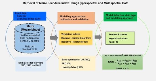
Field spectra acquired from a handheld spectroradiometer and Sentinel-2 images spectra were used to investigate the applicability of hyperspectral and multispectral data in retrieving the maize leaf area index in low-input crop systems, with high spatial and intra-annual variability, and low yield, in southern Mozambique, during three years. Seventeen vegetation indices, comprising two and three band indices, and nine machine learning regression algorithms (MLRA) were tested for the statistical approach while five cost functions were tested in the look-up-table (LUT) inversion approach. The three band vegetation indices were selected, specifically the modified difference index (mDI_{d: 725; 715; 565}) for the hyperspectral dataset and the modified simple ratio (mSR_{c: 740; 705; 865}) for the multispectral dataset of field spectra and the three band spectral index (TBSI_{b: 665; 865; 783}) for the Sentinel-2 dataset. The relevant vector machine was the selected MLRA for the two datasets of field spectra (multispectral and hyperspectral) while the support vector machine was selected for the Sentinel-2 data. When using the LUT inversion technique, the minimum contrast estimation and the Bhattacharyya divergence cost functions were the best performing. The vegetation indices outperformed the other two approaches, with the TBSI_b as the most accurate index (RMSE = 0.35). At the field scale, spectral data from Sentinel-2 can accurately retrieve the maize leaf area index in the study area.

1. Introduction

The leaf area index (LAI) is a parameter of crop structure, which is key for many agronomic and physiologic studies involving plant growth, light interception, photosynthetic efficiency, evapotranspiration, and plant response to irrigation, fertilization, and other types of agricultural practices [1]. The LAI describes the mass and energy exchange surface between the Earth’s surface and the atmosphere, influences the within and bellow canopy microclimate, and determines and controls the canopy water interception, the radiation extinction, and the water and carbon gas exchange [2]. Due to its role as an interface between the ecosystems and the atmosphere, studies involving LAI have applications in a wide range of fields, particularly in agriculture, forests, ecology, hydrology, eco-physiology, and meteorology [3,4].

Remote sensing data acquired from different types of sensors and processed through various modelling approaches have been revealing a high potential for retrieving and mapping LAI, which is an important contribution to the management of agricultural fields at different spatial and temporal scales [5,6,7]. The principle inherent to the application of spectral information for LAI (or other biophysical variable) retrieval is related to the changes in crop spectral behavior in response to variations of physiologic and structural conditions of plants as well as to the surrounding environment conditions [8].

Although data from a wide diversity of multispectral sensors is currently available, there are some limitations in their use for LAI retrieval due to the occurrence of saturation in high LAI conditions or high amounts of biomass [9,10,11]. Thus, there has been an increasing interest in the application of hyperspectral data. The numerous narrow bands of hyperspectral sensors provide continuous spectral measurement across the electromagnetic spectrum, which are more sensitive to subtle variations in reflected energy and, therefore, have a greater potential for detecting differences between surface characteristics [12]. Thus, through hyperspectral data it is possible to use narrow bands specifically suited for quantifying biophysical and/or biochemical variables of vegetation [13].

The estimation of plant biophysical variables using spectral data can be achieved through statistically (or empirical) and physically based approaches. The statistical techniques are used to analyze the relationship between variables of interest measured in situ and the crop spectral reflectance or its transformations in the form of vegetation indices or regression algorithms. Several studies have applied this approach to estimate different biophysical parameters of agricultural crops, including the estimation of LAI [14]. Although this approach is easy to implement and has been successfully applied in several studies, it is often site specific, i.e., the transferability of the resulting statistical relationship usually presents constraints when used under different conditions (locations, stages of crop development, agricultural practices, etc.), or with sensors of different characteristics, namely in their spectral resolution [15]. To cope with this limitation, it is necessary to ensure a broad sampling, considering different stages of crop development, different varieties (within a single crop), and different locations [16].

The statistical relationship between crop biophysical data and their reflectance is generally done through vegetation indices that may assume different formalisms: (i) Indices using single-band reflectance or the difference between two wavelengths; (ii) reflectance ratios between two or more bands; (iii) normalized difference ratios; and (iv) indices based on reflectance derivatives [14]. Alternatively, this relationship can be assessed using machine learning algorithms [17].

In the physical approach, methods of inversion of radiative transfer models (RTMs) are applied. The radiative transference is the physical phenomenon of energy transfer in the form of electromagnetic radiation, which is affected by the absorption, emission, and dispersion processes. The RTMs describe, based on physical laws, the temporal variation of canopy spectral reflectance as a function of its biochemical and structural properties coupled with the soil properties and the illumination conditions of the object [18]. For these reasons, this approach is considered more robust than the statistical. However, the application of RTMs, in addition to reflectance, requires supplemental information relative to canopy structure and reflectance of proximity objects, such as soil, to characterize the physical model and describe the conditions in which the model is valid. This information is not always available and, even when available, the reflectance simulation process is computationally demanding. These are the main limitations for the RTMs’ applicability [15]. Nevertheless, the RTMs have been applied in a great diversity of regions and types of vegetation, considering several types of sensors for the retrieval of different vegetation biophysical parameters.

The most commonly used RTMs for the estimation of vegetation biophysical properties are PROSPECT (leaf optical proprieties spectra) and SAIL (scattering by arbitrarily inclined leaves). The PROSPECT model, proposed by Jacquemoud and Baret [19], simulates the reflectance and transmittance of the leaf [20], and it is frequently coupled with the SAIL model to simulate the canopy’s bidirectional reflectance [12].

The combination of POSPECT and SAIL (PROSAIL) interconnects the variation of the spectral reflectance of the canopy, which is mainly related to the biochemical attributes of the leaf, with its directional variation, which is mainly related to the canopy architecture and the contrast between soil/vegetation. This linkage is essential for the simultaneous estimation of the biophysical and structural variables of the vegetation [21]. However, the parameterization of PROSAIL seems quite challenging in such a way that most of the studies use nominal values or ranges applied in other studies carried out with the same crops, but in different places. In

Table A1. Summary of PROSPECT and PROSAIL parameters as used in different studies.

Authors	[56]	[67]	[84]	[85]	[2]	[86]	[14]
Model: PROSPECT 5
Ca+b: Clorofila a+b (µg/cm²)	30–70	20–80	15–55	5–70	10–70	10–70	05–75
Equivalent water thickness (g/cm2)	0.01–0.06	0.01–0.04	0.01–0.02	-	-	0.01–0.03	0.002–0.05
N: Leaf Structural Parameter	1–3	1	1.5–1.9	1.5	1.3–1.7	1–1.6	1.3–2.5
Car: Carotenoids (µg/cm²)	-	1	-	-	-	-	-
Cbrown: Brown pigments (g/cm²)	-	0.05	-	-	-	0–2	-
Cm: Dry matter content (g/cm²)	0.008–0.025	0.0046	0.005–0.01	0.009	0.004–0.007	0.005–0.021	0.001–0.03
Model: 4SAIL
LAI: Leaf area Index	1–7	0.1–6	0.3–7.5	0–8	0–6	0–7	0.1–7
ALA: Leaf angle distribution (°)	20–60	70, 57, 45	40–70	35	40–70	40–70	40–70
skyl: Diffuse/Direct light	-	0.1	-	-	-	10	0.05
psoil: Soil Coefficient	-	0.1	0.5–1.5	-	0.7–1.3	0–1	0–1
hspot: Hot spot	0.5/LAI	0.78, 0.40, 0.32	0.05–0.1	0.01	0.05–1	1–1.6	0.05–0.5
tts: Solar Zenit Angle (°)	−20–+80	51, 45, 33	-	30	35	20–50	22.3
tto: Observer zenit Angle (°)	0–55	0	-	10	0	0	20.19
psi: Azimut Angle (°)	−120–+120	0	-	-	0	0	0
Crop/vegetation type	Wheat	Wheat	Rangelands	Maize, vegetables, sunflower, alfafa and vine	Maize and sugar beet	Maize, vegetables and alfafa	Maize, vegetables, alfafa, sunflower, vines

(Appendix A), we present the PROSPECT and SAIL models, including parameters used in several crops and vegetation types.

Overall, although several mentioned studies have achieved good results estimating and mapping crop biophysical properties through different remote sensing data and methods, according to [22], there are still gaps to be explored in terms of the use and operationalization of these data and methods. The diversity of bands selected for estimating the same variable, for the same crop, in different studies, and the variability of the intervals of parameters used in the calibration of the RTMs for the same crop, emphasize the impact of the radiometric characteristics of the sensors, the agricultural practices (which determine the canopy structure), the environmental conditions, and sampling conditions on the models’ results. This assumption is even more important when remote sensing data and methods are to be applied in low-input crop systems and highly heterogeneous farming systems, as is the case of the present study area. In this type of farming system, the limitation of the production factors, such as fertilizers and irrigation, leads to crops with very low LAI and high infield heterogeneity, which constitutes an additional challenge in the application of remote sensing techniques.

In this context, the main goal of this work is testing the applicability of different types of remote sensing data (hyperspectral and multispectral) and methods (statistical and physical) for developing models to predict LAI in maize crop systems characterized by low input factors, high spatial and intra-annual variability, and low yield in the south of Mozambique. The specific objectives include (i) to compare the performance of multi and hyperspectral data in estimating the LAI of maize in the study region; and (ii) to test the performance of the RTMs and the statistically-based models in the estimation of LAI of maize.

2. Materials and Methods

2.1. Study Area Description

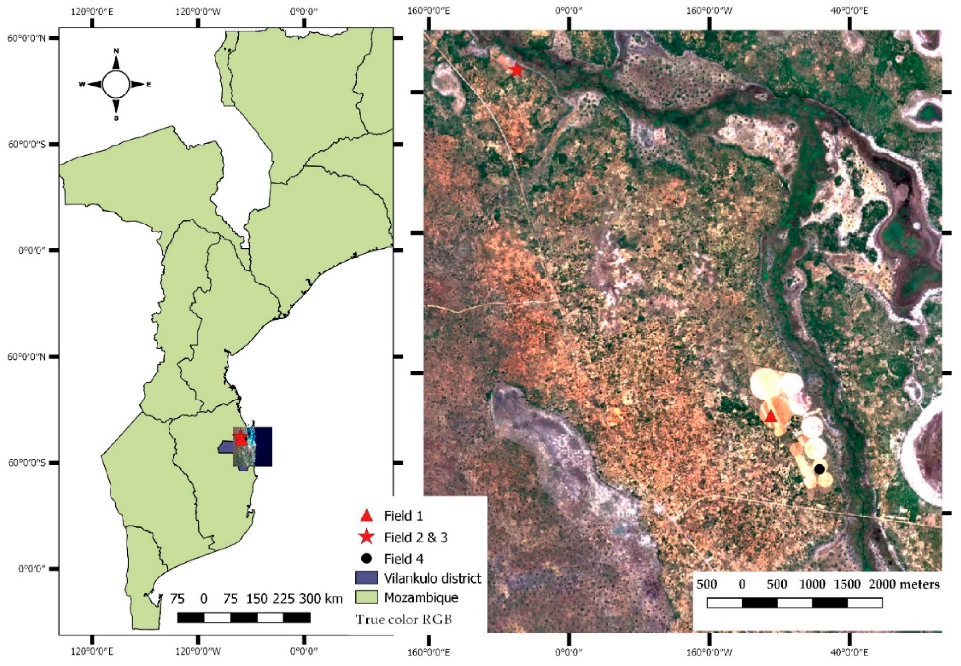
The current study was conducted in maize crop fields located in the district of Vilankulo, within the province of Inhambane in southern Mozambique (lat.: 21°58′S, long.: 035°09′E, 31.83 m a.s.l) (Figure 1).

The district of Vilankulo is characterized by a semi-arid to arid climate, with sandy soils of low fertility. Figure 2 presents the average precipitation and temperature in the study area for a reference period and for the three years of data collection. For the period studied (2015–2018), the average of total annual rainfall was 403 mm, which is 50% below the 804.4 mm registered in the period (1991–2015). The average annual temperature of 26.9 °C during the study period was warmer than that recorded in the period of 1991–2015 (24.5 °C). The summer and rainy season (January, February, March, October, November, and December) accounted for the highest amount of rainfall for both the reference period (79.8%) and study period (81.2%). The driest conditions were recorded in 2015 with 335.3 mm of total annual rainfall and an average temperature of 29.0 °C.

2.2. Characteristics of the Sampled Fields

The data collection took place in four maize fields in 2015 (field 1), 2016 (field 2 and field 3) and 2018 (field 4). In 2015 and 2016, the crop cycle coincided with the cold and dry season (April–September) while in 2018, the crop was grown during hot and rainy season. In each field, two 400 m² parcels were established for monitoring and data collection.

Table 1. Characteristics and main agricultural practices of the sampled fields.

Item	Field 1 (2015)	Field 2 (2016)	Field 3 (2016)	Field 4 (2018)
Latitude	21°56′24.19″	21°59′02.53″	21°56′20.88″	21°59′24.62″
Longitude	35°07′24.19″	35°09′30.95″	35°07′18.12″	35°09′55.53″
Surface	3 ha	1 ha	1 ha	3 ha
Soils	Sandy-loam soils	Sandy-loam soils	Sandy-loam soils	Sandy-loam soils
Irrigation system and scheduling	Sprinkler: irrigation schedule conditioned by the water pumping availability	Drip irrigation: 3 days interval from V3–V8 and 6 days interval in the following stages	Drip irrigation: 3 days interval from V3–V8 and 6 days interval in the following stages	Central pivot: 5 days irrigation interval (with punctual constraints due power fluctuations)
Variety	PAN 53, a medium maturity variety (125–140 days to harvest)	PAN 53	PAN 53	PAN 67, a medium maturity variety (120–130 days to harvest)
Planting geometry	0.5 × 0.25 cm;	0.75 × 0.2 cm;	0.75 × 0.2 cm;	0.9 × 0.15 cm;
Sowing and harvest dates	9 June/30 October	2 June/2 November	4 July/4 December	10 December 2017/25 April 2018
Crop yield	2.5 Ton/ha	5 Ton/ha	5 Ton/ha	4 Ton/ha
Agricultural practices	Surface fertilization with Urea; manual weed removal; insect control of insect Sesamia monogriodes with cipermetrine at stages V8, VT and R	Deep fertilization with Guano (1200 kg/ha) before sowing; 3 applications of Mono-Ammonium Phosphate (MAP) (200 kg/ha) and Ammonium Sulphate (100 kg/ha) throughout the season	Deep fertilization with Guano (1200 kg/ha) before sowing; 3 applications of Mono-Ammonium Phosphate (MAP) (200 kg/ha) and Ammonium Sulphate (100 kg/ha) throughout the season	Deep fertilization with Guano (1200 kg/ha) early before sowing; 3 applications of Mono Amonium-Phosphate (MAP) (200 kg/ha) and Ammonium Sulphate (100 kg/ha) throughout the season; application of insecticides to control the Spodoptera frugiperda

summarizes the cropping practices in each sampled field.

2.3. Data Collection

2.3.1. Field LAI Data Collection

The field LAI data was obtained from an allometric model, which estimates the plant total leaf area based on biometric variables (length and width) and the number of leaves. The model variables were collected during the years, 2015, 2016, and 2018, in seven plants randomly selected and marked within each parcel. The maize measurements (allometrics descriptors) were recorded in different crop phenologic stages (

Table 2. Dates of field leaf area index collection and corresponding crop phenological stages.

Crop Stage	Dates of Data Collection
	Field 1 (2015)	Field 2 (2016)	Field 3 (2016)	Field 4 (2018)
V3	2 July	28 Jun	30 July	9 January
V6	20 July	19 July	12 August	25/January
V8	31 July	30 July	24 August	5 February
VT	28 August	17 August	13 August	4 March
R1	3 September	28 August	27 September
RT		16 September	25 October

V3, V6, V8—stages at which the plants have 3, 6, and 8 leaves with visible leaves, respectively; VT—stage at which the last new leaf is completely developed; R1—first reproductive stage; RT—last reproductive stage.

) described in accordance with the leaf collar method [24]. This allometric model was calibrated and validated during the 2015 field campaign using the maize variety, ‘PAN 53’, and explained 90% of the maize total leaf area variability at different stages of crop development (R² = 0.90; n = 30; p < 0.000) [1]. Additionally, an independent validation of the model was performed using data from the crop variety, ‘PAN 67’, grown in 2018 (R² = 0.914, n = 16, p < 0.000; data not published).

2.3.2. Field Equivalent Water Thickness and Dry Mater Content

For the estimation of the equivalent water thickness (Cw,) and dry mater content (Cm, g/cm²), the first full developed leaf, defined from the top to the bottom of each sampled plant, was cut and enclosed in a sealed plastic bag and brought to the laboratory inside a cooler. In the laboratory, a 2 cm diameter disc was cut in each leaf and the wet weight taken before the discs were dried at 65 °C in an oven until constant weight (dry weight). The Cw (cm) was then calculated according to the following equation:

$$\mathrm{Cw}=\frac{{\mathrm{F}}_{\mathrm{w}}-{\mathrm{D}}_{\mathrm{w}}}{\mathrm{A}}\times \mathrm{dw}$$

(1)

where F_w (g) and D_w (g) are, respectively, the fresh and dry weights of the leaf discs; A (cm₂) is the area of the disc; and dw (1 g cm⁻³) is the water density. For the estimation of Cm, we used the following equation:

$$\mathrm{Cm}=\frac{{\mathrm{D}}_{\mathrm{w}}}{\mathrm{A}}$$

(2)

2.3.3. Field Spectral Data Collection

The field spectral data were acquired using an Apogee hyperspectral spectroradiometer with sensitivity in the range of 236 nm–1100 nm and a spectral resolution of 1 nm. The instrument is attached to an optic cable with a field of view (FOV) of 30°. The measurements were taken at the nadir position, keeping a constant distance of about 5 cm to the spot, and were carried out around solar noon (between 11 a.m. and 1 p.m.), when the changes in solar zenith are minimal. Standard procedures of the equipment calibration were followed, namely the dark object correction and the acquisition of white reference reflectance of the Spectralon. The reference reflectance was updated every 10 min during the measurements. The spectra readings were done in the same dates (Table 2) and points where the data for LAI determination were collected. In the phenological stages, V3, V6, and V8, while the fraction of canopy cover was still very low, two additional readings were done, one over the interface between two plants and another over bare soil. In each point, 10 replications were made, with each an average of 20 automatic readings.

2.3.4. Spectral Data from Sentinel-2

The multispectral sensors imaging (MSI) on board of the Sentinel-2A and Sentinel-2B, launched, respectively, in June 2015 and March 2017, have a temporal resolution of 10 days and present 4 bands (2, 3, 4, and 8) with 10 m of spatial resolution and 6 bands (5, 6, 7, 8a, 11, and 12) with 20 m of spatial resolution. The high spatial and temporal resolutions and the spectral intervals covered by these bands make Sentinel-2 potentially more interesting than other multispectral sensors for studies related with LAI [25,26,27].

Atmospherically corrected Sentinel-2A and Sentinel-2B images of the study area, including their value added product bands, were acquired from the data service platform developed by [28]. For all the pixels covering each sampling parcel, the spectral data of all the original Sentinel-2 bands (SP_S2) and of the Sentinel LAI products (LAI_S2) were extracted and then averaged, using a 10 m spatial filter applying the zonal statistics tool of QGIS software, version 2.14.14. The Sentinel-2 images were selected considering the closeness to field spectral data collection dates and low cloud cover. The images from the following dates were then selected and downloaded: 30/06/2016; 20/07/2016; 30/07/2016/; 28/09/2016; 21/01/2018; 05/02/2018, and 02/03/2018. The dates of satellite acquisition and field data collection did not always match due to frequent high cloud cover conditions in the study area at the time of satellite overpass. However, nearby satellite image dates, corresponding to the same crop phenological stage, were always considered.

2.4. Data Analysis

2.4.1. Field Spectral Data Pre-Processing

The reflectance of each sampling point was achieved by averaging the 10 replications. For the stages, V3, V6, and V8, the average included the reflectance of the plant, bare soil, and interface between two plants. A weighted average of the three ground cover components was considered to obtain a reflectance value representative of maize growth conditions at each sampling point and allow the comparability with satellite data. Due to noise in the initial portion of the spectra, data analysis was performed considering data in the interval of 400 nm–1100 nm of the spectra. Afterwards, these data were spectrally aggregated to simulate hyperspectral and multispectral datasets. For the hyperspectral dataset, a 10 nm spectral resolution aggregation (FSP_10) was considered while for the multispectral dataset, the Sentinel-2 band setting was used for aggregation (FSP_S2). Because the field spectra does not match the whole Sentinel-2 spectra, the aggregation was limited to 8 bands (2 A–8 A) acknowledged as being more convenient in LAI estimations [2,29].

2.4.2. Statistical Modelling of LAI Based on Vegetation Indices

Table 3. Spectral vegetation indices tested for statistical LAI modelling.

Type of Index	Formulation	Original Index and Source
2 bands index
ND	(ρ a − ρ b)/(ρ a + ρ b)	NDVI; [31]
mNDa	[(ρ a − ρ b)/(ρ a + ρ b + 0.5)] * 1.5	SAVI; [32]
SR	ρ a/ρ b	SR; [33]
mSRa	ρ a/ρ b − 1	CI Green; [34]
DI	ρ a − ρ b	DI; [35]
mDIa	(1/ρ a) − (1/ρ b)	ARI; [36]
3 bands index
mDIb	(ρ a − ρ b) − 0.2 * (ρ a − ρ c)	CARI; [37]
mNDb	2.5 * [(ρ a − ρ b)/(ρ a + 6 * ρ b + 7.5 * ρ c + 1)]	EVI; [38]
mNDc	(ρ a − ρ b)/(ρ a + ρ b − ρ c)	VARI; [39]
mSRb	(ρ a − ρ b)/(ρ a − ρ c)	SIPI; [40]
mSRc	(ρ a − ρ b)/ρ c	PSRI; [41]
mDIc	[(ρ a − ρ b) − 0.2 * (ρ a − ρ c)] * (ρ a/ρ b)	mCARI; [42]
mDId	[(1/ρ a) − (1/ρ b)] * ρ c	mARI; [36]
mDIe	[(ρ a + ρ b)/2] − ρ c	RVSI; [43]
TBSIa	(ρ a − ρ c)/(ρ b + ρ a)	[14]
TBSIb	(ρ a − ρ b + 2 ρ c)/(ρ a + ρ b + ρ c)	[44]
TBSIc	(ρ a − ρ b − ρ c)/(ρ a + ρ b + ρ c)	[45]

ρ—Reflectance at given wavelength; SR—simple ratio; ND—normalized difference; mSR—modified simple ratio; mND—modified normalized difference; TBSI—three band spectral index; DI—difference index; EVI—enhanced vegetation index; SAVI—soil adjusted vegetation index; NDVI—normalized difference vegetation index; VARI—visible atmospherically resistant index; CARI—chlorophyll absorption ratio index; mCARI—modified chlorophyll absorption ratio index; CI_Green—green chlorophyll index; ARI—anthocyanin reflectance index; mARI—modified anthocyanin reflectance index; SIPI—structure insensitive pigment index; PSRI—plant senescence reflectance index; RVSI—reflectance vegetation stress index. Figure 3 presents the flowchart of the two statistical modelling approaches.

presents the spectral vegetation indices (VI) assessed as predictors for LAI statistical modelling. The VIs included band combinations in the form of the simple ratio (SR), modified simple ratio (mSR), normalized difference (ND), modified normalized difference (mND), difference between bands (DI), and modified difference between bands (mDI). For each VI, all possible band combinations were tested considering the three types of data: Hyperspectral dataset (FSP_10), the multispectral dataset (FSP_S2), and the Sentinel-2 data (SP_S2). The FSP_10 and FSP_S2 were correlated only to the field leaf area index (Field_LAI) while the SP_S2 was correlated to both the average Field_LAI and Sentinel-2 leaf area index product (LAI_S2). The linear, exponential, and second degree polynomial functions were evaluated for modelling the LAI based on VIs. The analysis of the best band combination per VI and the modelling approach were carried out in the Spectral Index Toolbox of the software Automated Radiative Transfer Models Operator (ARTMO) [15,30].

2.4.3. Statistical Modelling of LAI Based on Machine Learning Regression Algorithms

The machine learning regression algorithms (MLRA) are nonparametric models that are adjusted to predict a variable of interest using a training dataset of input-output data pairs, derived from synchronised measurements of the parameter and the corresponding reflectance observations. Numerous nonparametric regression algorithms are available in the statistics and machine learning literature, and they are being increasingly applied for vegetation biophysical parameters’ retrieval [14,16,17,46,47].

Similarly to the VIs, the MLRA algorithms were evaluated using the three types of data: Hyperspectral dataset (FSP_10), multispectral dataset (FSP_S2), and Sentinel-2 data (SP_S2). The FSP_10 and FSP_S2 were correlated only to the field leaf area index (Field_LAI) and the SP_S2 was correlated to both the Field_LAI and Sentinel-2 LAI product (LAI_S2).

Table 4. Machine learning regression algorithms tested for LAI modelling.

Algorithm	Source
Regression tree (RT)	[48]
Random Forest (TreeBagger) (RFTB)	[49]
Bagging trees (BaT)	[50]
Relevance vector machine (RVM)	[51]
Kernel ridge regression (KRR)	[52]
Gaussian process regression (GPR)	[53]
Variation Heteroscedastic Gaussian process regression (VH-GPR)	[54]
Support Vector Regression (SVM)	[55]
Random Forest (Fitensemble) (RFF)	[49]

presents the MLRA evaluated in the present study and the modelling process is presented in Figure 3. Prior to the application of the MLRA algorithms, an analysis of the best number and combination of bands for estimating the LAI using the different datasets was performed based on the band analysis toolbox. The algorithms were also implemented on the MLRA toolbox [17] of the software Automated Radiative Transfer Models Operator (ARTMO).

2.4.4. Retrieval of LAI Based on Radiative Transfer Models

To perform an LAI retrieval through RTMs, one need to first build up a look-up-table (LUT), which is a database of simulated canopy reflectance and their corresponding set of input parameters. Afterwards, an inversion technique is applied to search and identify the parameters’ combination that yields the best fit between the measured and LUT reflectance [18,56].

Simulation of the Look-Up-Table (LUT)

The PROSAIL model, a widely used RTM model for biophysical parameters’ retrieval [14,57], was used to simulate reflectance data that were stored in an LUT.

Table 5. Input parameters of PROSAIL used to generate LUT for maize in the study area.

Model/Parameter	Abbreviation	Unit	Range of Values	Fixed Values
Prospect 5 model
Equivalent water thickness	Cw	cm	0.001–0.030	-
Leaf chlorophyll content	Cab	µg/cm²	5–40	-
Leaf structure coefficient	N	No dimension	1–1.4	-
Dry matter content	Cm	g/cm2	0.001–0.008	-
Carotenoids content	Car	µg/cm²	-	10
Brown pigments content	Cbrown	g/cm²	-	5
4SAIL model
Leaf area index	LAI	m2/m2	0.01–3.5	-
Average leaf angle	ALA	Degree	20–60	-
Hot-spot size parameter	Hspot	m/m	0.25–1	-
Diffuse/Direct light	Skyl	No dimension	-	10
Soil Coefficient	Psoil	No dimension	-	0.6
Solar Zenith Angle	Tts	Degree	-	10
Observer zenith Angle	Tto	Degree	-	5
Azimuth Angle	Psi	Degree	-	0

presents the input parameters’ settings used for the LUT simulations. The input parameters relative to LAI, water equivalent thickness (Cw), dry matter content (Cm), hotspot (hspot), and the reflectance of dry and wet soil were set according to field data. The parameter of leaf structure (N) was set to the 1–1.4 interval as proposed by [2,58,59] for various crops, including maize. The interval of values considered for the chlorophyll a and b content (Ca+b) was defined slightly below the ranges presented in the current literature considering the local conditions, which are prone to stress occurrence due to irrigation deficit conditions and damages by insects. As mentioned by several authors, when plants are exposed to stress (water deficit, insect damage, nutrient deficit, etc.), the pigments’ concentration is reduced and/or degraded [60,61,62], lowering the energy absorption and thus increasing the reflectance in the visible domain. The observer zenith angle (tto), the azimuth angle (psi), and the sun zenital angle (tts) were set according to the geometry of field spectra readings.

A total number of 100,000 random simulations was used for generating the LUT spectral reflectance data. This simulations’ number is considered appropriate for good computational efficiency and high accuracy in the parameter estimation [63,64,65]. The simulated data were aggregated into the eight Sentinel-2 bands (2–8 A) in order to match the FSP_S2 dataset. The PROSAIL simulations were carried out in the software, ARTMO [30].

LUT Inversion for LAI Retrieval

A look-up table (LUT) based inversion technique was applied for the LAI retrieval. This technique is considered easy-to-use and potentially outperforms the limitations of iterative techniques [63,66]. The LUT inversion consists of a direct comparison of simulated spectral data with the observed spectral data (field or satellite data), through one or various cost functions, aiming to identify the best parameter combinations that yield minimal differences between the observed and simulated data [14,67]. The LUT inversion toolbox [68] of the ARTMO software was used to perform this inversion task. The toolbox enables testing simultaneously a wide diversity of cost functions making it possible to optimize the models for different assumptions on the nature and proprieties of the residuals [68,69]. Several classes of cost functions were considered, including minimum contrast estimation, information measures, and M-estimates.

The minimum contrast estimation considers the bidirectional reflectance as a spectral density of the stochastic process and aims at minimizing the distance between a parametric model and a non-parametric spectral density [69]. Within this class, three cost functions were tested, which are detailed in [69,70]:

$$K\left(x\right)=-logx+x, then, D\left[E,L\right]={\displaystyle \sum }_{\lambda =1}^{\lambda n}\left[-\log \left(\frac{l\left(\lambda i\right)}{e\left(\lambda i\right)}\right)+\left(\frac{l\left(\lambda i\right)}{e\left(\lambda i\right)}\right)\right]$$

(3)

$$K\left(x\right)={(logx)}^2, D\left[E,L\right]={\displaystyle \sum }_{\lambda =1}^{\lambda n}{[\log (l(\lambda i)-log(e(\lambda i))]}^2$$

(4)

$$K\left(x\right)=xlogx-x, then, D[E,L]={\displaystyle \sum }_{\lambda =1}^{\lambda n}l(\lambda i)e{(\lambda i)}^{-1}\{\log (l(\lambda i)e{(\lambda i)}^{-1})-1\}$$

(5)

where, $D\left[E,L\right]$ is the distance between two functions, $E=\{e(\lambda i), \dots , e(\lambda n)\}$ is the FSP_S2 or the SP_S2 datasets, $L=\{l(\lambda i), \dots , l(\lambda n)\}$ is the PROSAIL simulated reflectance (LUT), and, $\lambda i, \dots , \lambda n$ is the spectral bands.

The information measures represent measures of distance between two probability distributions. The reflectance is interpreted as a function of probability distribution [68]. In this class, the Bhattacharyya divergence [69] was tested:

$$D\left[E,L\right]=-\log +\{{\displaystyle \sum }_{\lambda i=1}^{\lambda n}\sqrt{e(\lambda i)l(\lambda i)}-\frac{1}{2}(e(\lambda i)+l(\lambda i))\}$$

(6)

The M-estimate measures rely on minimizing a dispersion function. Even though the M-estimates are the most commonly used measures, they can be misleading if their basic assumptions of residual normality and absence of extreme values are not met [69]. In this class, we tested the root mean square error (RMSE), which is calculated as:

$$\mathrm{RMSE}:D\left[E,L\right]=\sqrt{\frac{{{\displaystyle \sum }}_{\lambda i=1}^{\lambda i=n}{(e(\lambda i)-l(\lambda i))}^2}{n}}$$

(7)

Figure 4 presents the scheme of the LUT generation and the inversion process for LAI retrieval.

2.5. LAI Model Calibration, Cross Validation, and External Validation

Data from 2016 were used for the calibration of statistical models (VI and MLRA) because it covered more crop phenological stages and a larger number of observations than the datasets of the other study years (2015 and 2018) (Table 2), resulting in high data variability.

In the VI approach, the calibration consists in a systematic assessment of all possible band combinations, vegetation indices formulations (Table 3), and curve fitting options. This process yields a table of goodness-of-fit measures for the values estimated by the calibrated model against the measured calibration measures [15]. A validation process is simultaneously performed. In this study, we used a k-fold cross validation method, which involves randomly dividing the dataset into k equal-sized sub-datasets. From these k sub-datasets, k − 1 sub-datasets are used as a training dataset and a single k sub-dataset is used as a validation dataset for model testing. The cross-validation process is then repeated k times, with each of the k sub-datasets used as a validation dataset [14]. The results from each of these iterative validation steps are then combined to derive a single estimation value. At the end, all data are used for both training and validation, and each single observation is used for validation exactly once [14,71]. In this study, we used k = 2 and run the calibration/validation process several times until no improvement of the goodness-of-fit statistics were detected in both the calibration and validation processes.

In the MLRA approach, we first used the Gaussian process regression band analysis tool (GPR-BAT) to identify the most sensitive bands to LAI and the minimum number of bands for an acceptable estimate accuracy [17]. Subsequently, we tested nine algorithms using the identified bands for each dataset. We equally used a k = 2 k-fold cross validation process and ran it several times until no improvement of the results were obtained.

For both VI and MLRA, an external validation was performed using a dataset comprising data collected in 2015 and 2018 to assess the model transferability. However, the external validation was not run for the SP_S2 dataset due to the limited number of observations (n = 22).

2.6. Model Assumptions, Accuracy Assessment, and Selection

The assumption of residual normal distribution was assessed by the Jarque-Bera (JB) test [72], and the Breusch-Pegan (BP) test [73] was used to investigate the presence of homoscedasticity, testing the dependence of the residuals’ variance on the independent variables. For JB tests, the null hypothesis is that the variance of the residuals is normally distributed while for the BP, the null hypothesis is that the residuals are homogeneous. Thus, for p-values less than 5%, we reject the null hypothesis. The models’ performance was assessed through three widely used statistical measures: The root mean square error (RMSE), the relative root mean square, and the coefficient of determination (R²). These measures were compared within the different retrieval approaches (VI, MLRA, and LUT inversion) and between them to decide which approach performed better in estimating LAI in the study area.

3. Results

3.1. LAI Ground Measurements and Derived from Sentinel-2

Figure 5 shows the intra-annual and inter-annual variability of LAI and a comparison between Field_ LAI and LAI_S2 in the study area. The LAI values ranged from 0.23 to 2.68 (averaging 1.34) in 2015, 0.32 to 3.54 (averaging 1.63) in 2016, and 0.49 to 2.28 (averaging 1.38) in 2018.

In 2016 the data collection covered the entire crop growing cycle (Table 2) and thus has an extended range and high average value of LAI, when compared with the data collected in the other two years. Also, the diversity between fields (sowing and irrigation conditions and crop treatments; Table 2) as well as the inter-annual weather conditions (Figure 2) likely contributed for the inter-annual LAI variability. The LAI_S2 that comprises data extracted from Sentinel-2 images acquired in 2016 and in 2018 ranged from 0.21 to 1.90 (averaging 0.61) and is very low if compared to the Field_LAI. A correlation between the Field_LAI and LAI_S2 yielded r = 0.69 (n = 30; p-value = 0.0001). This low correlation between measured and Sentinel derived LAI could be explained by several factors, including the scale mismatch and the fact that the LAI_S2 product was not validated in the context of our study area, which has very peculiar characteristics in terms of cropping systems (large in-field heterogeneity) with low LAI and soil background effects (soils with white colour). Also, the temporal mismatch between some LAI_S2 and Field_LAI data, due to cloud cover issues, may have also impacted the correlation between the two LAI products. Nevertheless, the S2 images’ acquisition dates are in agreement with the same crop growing stages as those of field data collection dates, minimizing this time effect.

3.2. Vegetation Index Based LAI Models and Validation

3.2.1. Field Spectral Data Resampled to 10 nm (FSP_10)

The model (FSP_10 vs. Field_LAI) goodness-of-fit statistics of the three best performing VIs in the calibration, cross validation, and external validation dataset are shown in

Table 6. Goodness-of fit statistics of the best performing vegetation indices (VI), using different combinations of spectral and leaf area index data.

VI	Bands	CA			CV			EV			Equation Parameters
		RMSE	R2	NRMSE	RMSE	R2	NRMSE	RMSE	R2	NRMSE
FSP_10 vs. Field_LAI
Observations		137			137			63
mSRb	735;565;715	0.39	0.85	13.4	0.41	0.83	16.2	0.8	0.8	20.8	a2 = 0.07; a1 = −1.056; a0 = 4.65
mDId	725;715;565	0.4	0.84	14.7	0.42	0.82	15.3	0.58	0.62	21.6	a2 = −319.73; a1 = −64.78; a0 = −0.59
mSRa	705;755	0.47	0.78	15.8	0.49	0.76	17.1	1.74	0.58	19.4	m = −6.05; b = −0.17
FSP_S2 vs. Field_LAI
Observations		137			137			63
mDIc	705;740;865	0.41	0.83	12.6	0.42	0.83	13.4	0.77	0.71	22.4	a2 = −587.33; a1 = −75.51; a0 = 0.37
mSRc	740;705;865	0.4	0.84	12.4	0.43	0.82	14.7	0.62	0.82	23.6	a2 = −21.63; a1 = 17.03; a0 = −0.63
mSRb	842;783;705	0.43	0.82	14.9	0.44	0.8	15.3	0.97	0.75	21.8	m = −6.87; b = 3.33
SP_S2 vs. Field_LAI
Observations		22			22
TBSIb	665;865;783	0.32	0.79	19.2	0.35	0.74	16.1	-	-		a2 = 166.6; a1 = 199.5; a0 = 59.9
mDIc	865;665;705	0.36	0.74	20.3	0.38	0.71	17.4	-	-		m = 3.1; b = −0.76
TBSIc	865;665;783	0.36	0.73	20.5	0.38	0.71	19.8	-	-		m = 9.6; b = 2.6
SP_S2 vs. LAI_S2
Observations		22			22
TBSIb	705;842;560	0.14	0.83	11.2	0.18	0.76	11.7	-	-		k = −2.9; n = 0.83
SR	665;783	0.18	0.73	12.4	0.19	0.72	11.5	-	-		m = 0.20; b = 0.9
TBSIa	560;705;842	0.17	0.75	12.2	0.19	0.73	10.3	-	-		m = −1.07; b = −0.16

CV—cross validation; EV—external validation; FSP_10—field spectral data resampled to 10 nm; FSP_S2—field spectral data resampled to Sentinel-2 bands; SP_S2—Sentinel-2 spectral data (SP_S2); Field_LAI—field leaf area index; LAI_S2—Sentinel-2 leaf area index product data; mSR—modified simple ratio; mDI—modified difference index; SR—simple ratio; TBSI—three band spectral index; a₀, a₁, a₂—coefficients of the second degree polynomial function (y = a₂X² + a₁X + a₀); m, b—coefficients of the linear function (y = mX + b); k, n—coefficients of the exponential equation (y = ne^kx); m, b—coefficients of the linear function (y = mX + b).

. The mSR_b and mDI_d fitted to a second degree polynomial function outperformed the other VI, showing consistent results for the LAI estimations when applied to the calibration, cross validation, and external validation datasets. For the external validation dataset, the mSR_b presents R² = 0.80, comparatively higher than the mDI_d (R² = 0.62), while the RMSE = 0.80 of mSR_b shows lower accuracy than the mDI_d with RMSE = 0.58. The three bands of VI, mSR_b, and mDI_d include bands within the same spectral regions of the green (565 nm) and red edge (715 nm, 725 nm, and 735 nm), suggesting reliability of the band optimization process for LAI estimation.

Figure 6 presents the agreement between the LAI measured and estimated with FSP_10 using the mSR_b and the mDI_d for the cross validation and external validation datasets. For the cross-validation dataset (Figure 6 left panel), the two indices exhibit good matching in the whole range of LAI values, but there is an underestimation for values greater than three. For the independent validation dataset (Figure 6 right panel), the two VIs estimate well the lower values of LAI, but for values above one, the estimation is poorer with an underestimation for the mDI_d and an overestimation for the mSR_b.

3.2.2. Field Spectral Data Resampled to Sentinel-2 (FSP_S2)

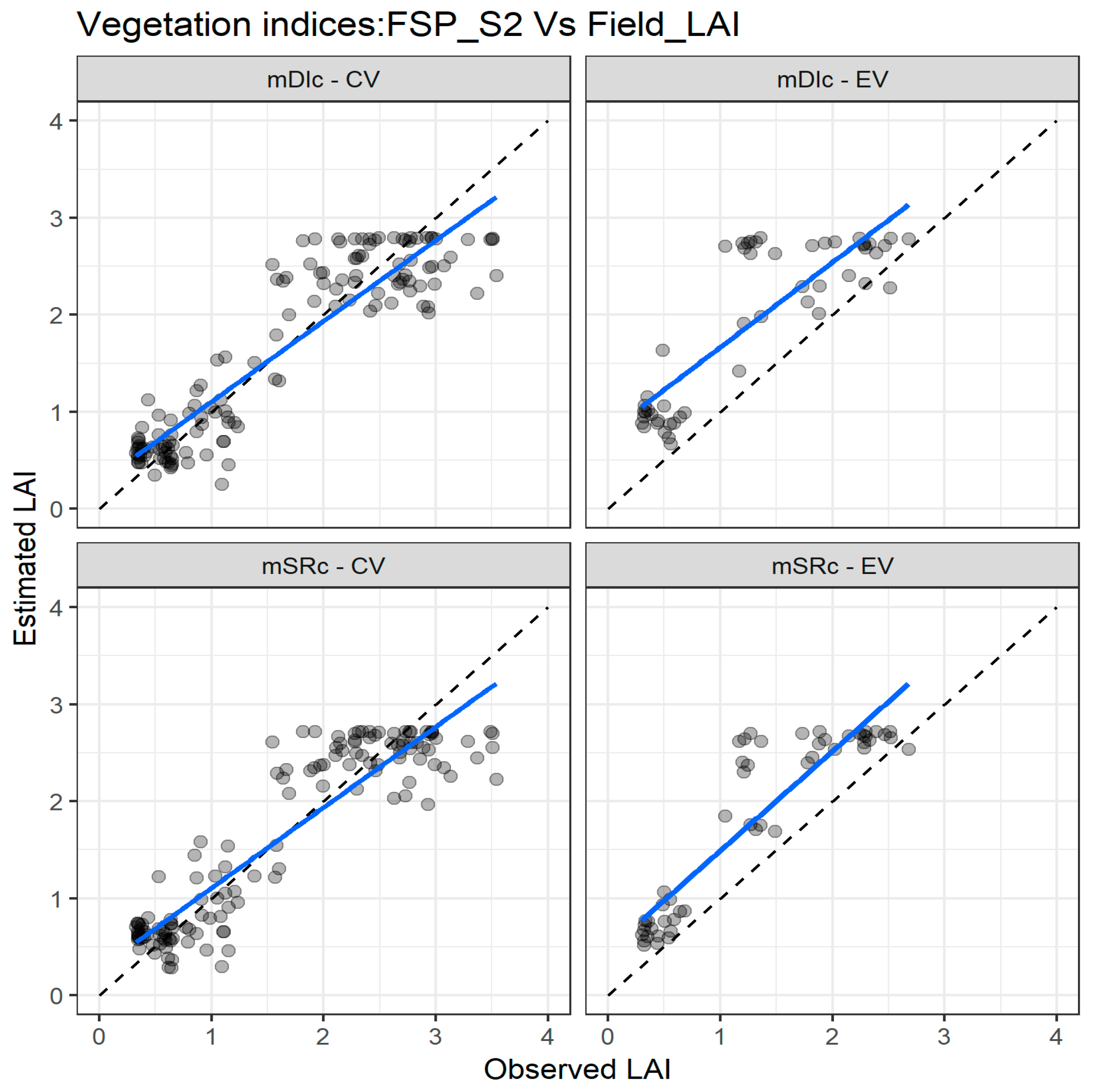
The goodness-of-fit statistics of the three best performing VIs for LAI estimation in calibration, cross validation, and external validation with the FSP_S2 is also presented in Table 6 (FSP_S2 vs. Field_LAI). The mSR_c, based on the polynomial model with bands located at the red edge (705 nm, 740 nm) and near infrared (865 nm) region of the spectra, presents better LAI estimates with R² ≥ 0.82 and RMSE of 0.40, 0.43, and 0.62, respectively, for the calibration, cross validation, and external validation datasets. The mDI_c presents very similar statistics for the calibration and cross validation datasets, but relatively lower R² (0.71) and higher RMSE (0.77) for the independent dataset. It is interesting to note that all the validated VIs derived from FSP_S2 were based on bands within the red edge and near infrared region of the spectra, which may suggest consistency of the band optimization and selection process.

Figure 7 depicts the agreement between measured and estimated LAI for the cross validation and external validation datasets. In the cross validation, there is a good agreement between measured and estimated LAI for the two indices, especially for LAI values below 2. As with the FSP_10 dataset, there is a miss match trend for LAI values higher than 2, which is more pronounced when the external dataset is used (Figure 7).

3.2.3. Sentinel-2 Spectral Data (SP_S2)

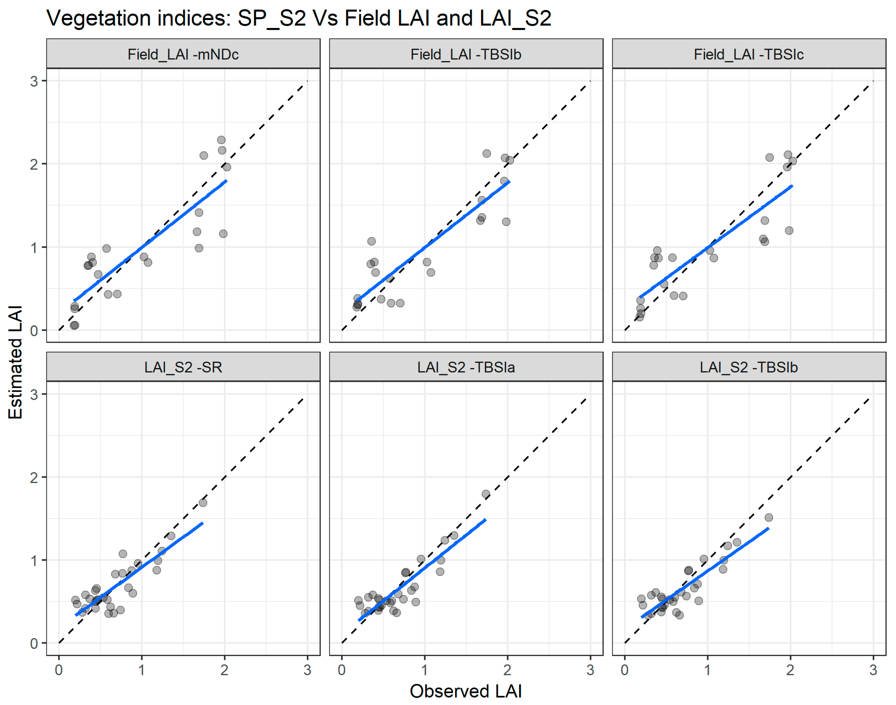
The goodness-of-fit statistics of the three best performing VIs for LAI estimation in calibration and cross validation for both SP_S2 vs. Field_LAI and SP_S2 vs. LAI_S2 are also presented in Table 6. For the SP_S2 vs. Field_LAI combination, the selected VIs (TBSI_b, mDI_c, TBSI_c) present very similar statistics and all were constructed with the same spectral bands, centred at red (665 nm), the red edge (783 nm), and near infrared (865 nm). However, the TBSI_b fitted to a second degree polynomial function outperforms the other VIs with an RMSE = 0.32, R² = 0.79 and RMSE = 0.35, R² = 0.74 for calibration and cross validation, respectively.

The SP_S2 vs. LAI_S2 combination presents excellent statistics for the three selected VIs (TBSI_b, SR_, TBSI_a), with the TBSI_b the outperforming one with an RMSE = 0.14, R² = 0.83 and RMSE = 0.18, R² = 0.76, respectively, for calibration and cross validation. This was expected because the SP_S2 was used as input data to derive the LAI_S2 products. However, careful interpretation is recommended given the lower correlation between the Field_LAI and the LAI_S2 (r = 0.69). The TBSI_b was constructed with green (560 nm), red edge (705 nm), and near infrared (865 nm) bands.

Figure 8 depicts the agreement between measured and estimated LAI for the cross validation with the two combinations: SP_S2 vs. Field_LAI (upper panel) and SP_S2 vs. LAI_S2 (lower panel). Clearly, the SP_S2 vs. LAI_S2 combination presents better agreement with the measured and estimated LAI.

3.3. Machine Learning Regression Based LAI Models and Validation

3.3.1. Field Spectral Data Resampled to 10 nm (FSP_10)

The LAI estimation based on MLRA was preceded by a band analysis tool in order to select the most sensitive bands among the initial number of 70 bands included in the FSP_10 dataset. The results indicated that increasing the number of bands in the models reduces the LAI estimation accuracy. Indeed, the maximum average R² (0.77) was obtained with three band models while the minimum average R² (0.70) was acquired with the total number of bands that comprises the hyperspectral dataset (70 bands) (Figure A1, Appendix A). The three selected bands are centered at 565 nm, 675 nm, and 775 nm, with a 10 nm spectral resolution, corresponding to green, red, and red edge regions of the spectra, respectively.

Table 7. Goodness-of-fit statistics for the LAI models of the best performing machine learning regression algorithms (MLRA) applied to different combinations of spectral and leaf area index.

MLRA/Type of Data	CV			EV
	RMSE	R2	NRMSE	RMSE	R2	NRMSE
FSP_10 vs. Field_LAI
Observations	137			63
Support Vector Regression (SVM)	0.48	0.77	14.9	0.67	0.65	17.5
Variation Heteroscedastic Gaussian Processes Regression (VHGPR)	0.53	0.73	16.5	0.63	0.83	16.3
Relevance vector Machine (RVM)	0.54	0.72	16.7	0.5	0.67	13.9
FSP_S2 vs. Field_LAI
Observations	137			63
Support Vector Regression (SVM)	0.48	0.78	14.9	0.9	0.72	24.9
Relevance vector Machine (RVM)	0.52	0.73	26.3	0.53	0.62	15.9
Bagging trees (BaT)	0.63	0.63	19.5	0.64	0.72	19.9
SP_S2 vs. Field_LAI (n = 22)
Observations	22			-
Support Vector Regression (SVM)	0.51	0.52	27.6	-	-
Random Forest (Fitensemble)	0.52	0.51	28.4	-	-
Gaussian Processes Regression (GPR)	0.5	0.49	27.4	-	-
SP_S2 vs. LAI_S2 (n = 22)
Observations	22			-
Random Forest (Fitensemble)	0.22	0.64	14.1	-	-
Relevance vector Marchine (RVM)	0.23	0.61	14.8	-	-
Support Vector Regression (SVM)	0.23	0.6	14.9	-	-

CV—cross validation; EV—external validation; FSP_10—field spectral data resampled to 10 nm; FSP_S2—field spectral data resampled to Sentinel-2 bands; SP_S2—Sentinel-2 spectral data (SP_S2); Field_LAI—field leaf area index; LAI_S2—Sentinel-2 leaf area index product data.

presents the goodness-of-fit statistics of the three best performing MLRA for LAI estimation using the three above mentioned bands. The relevance vector machine (RVM) algorithm shows better consistency for LAI estimation in both cross validation and external validation datasets.

With the cross validation dataset, the RVM has an RMSE = 0.54, which is higher than the values of RMSE of other MLRA; nevertheless, the RVM strongly outperform the other algorithms when used in the independent dataset with an RMSE = 0.50, which is clearly better compared to, for example, the SVM (RMSE = 0.67). The very high Gaussian process regression (VHGPR) also presented a good performance for the LAI estimation, both with the cross validation and external validation, although with a higher RMSE (0.63), when compared with the RVM algorithm for the external validation dataset.

Figure 9 depicts the comparison between measured and estimated LAI values for cross validation and external validation for the two best performing MLRA with the FSP_10 dataset. For cross validation (Figure 9 left panel), the two algorithms achieved good agreement in the entire LAI range, but there is a slight underestimation for LAI values above two. For the external validation dataset (Figure 9 right panel), the two algorithms exhibit good estimation in the full range of LAI values, although the VHGPR has lower accuracy for values exceeding two.

3.3.2. Field Spectral Data Resampled to Sentinel-2 Bands (FSP_S2)

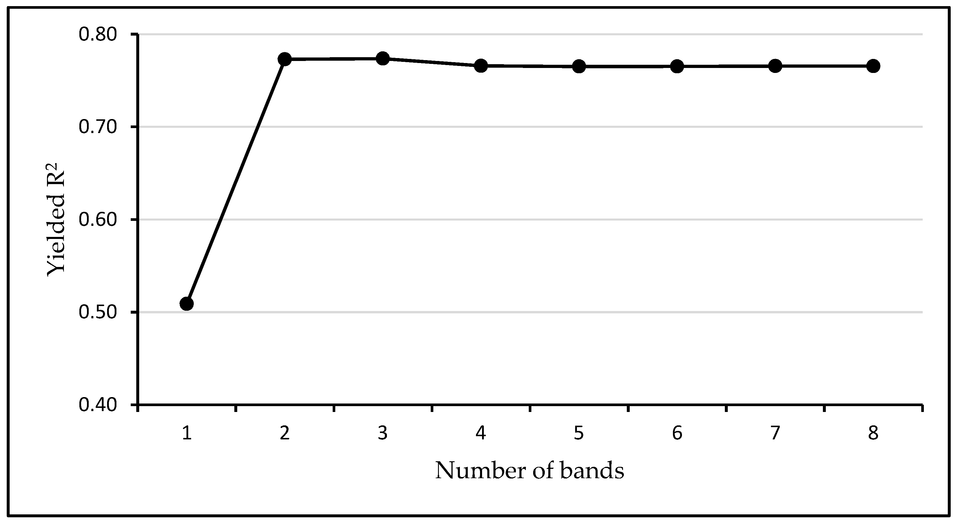
A band analysis was also performed prior to the MLRA assessment to select the best bands of the eight comprising the FSP_S2, for the LAI estimation. The results indicated that the LAI estimation accuracy increases from a minimum average of R² = 0.51, when only one band is involved, to a maximum average of R² = 0.77 when three bands are involved in the modelling (Figure A2, Appendix A). There was no accuracy improvement with additional band inclusion in the models. The selected bands match to the red and red edge Sentinel-2 bands, centered at 665 nm, 705 nm, and 783 nm.

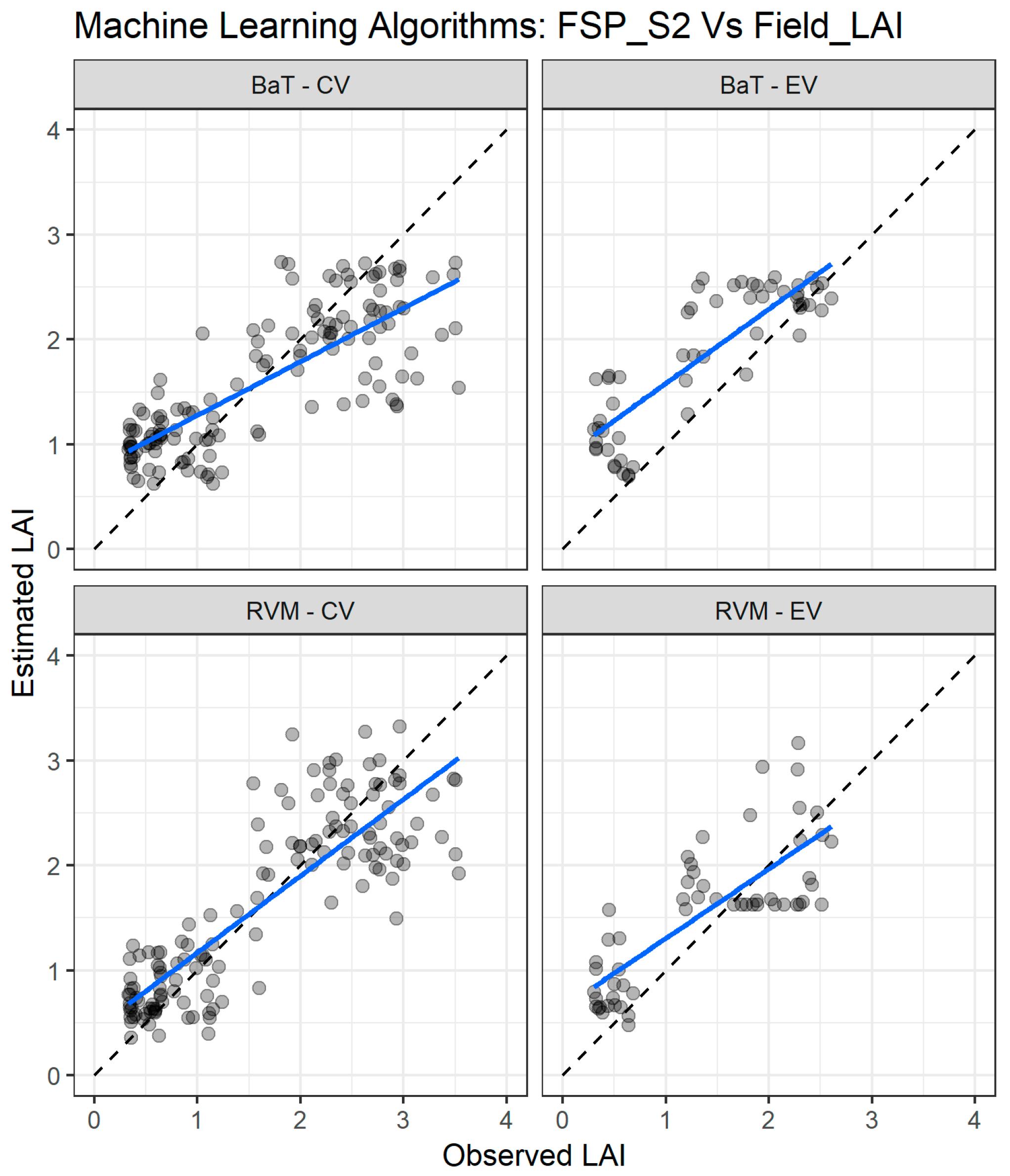
The goodness-of-fit statistics of the three best performing MLRA when using the FSP_S2 dataset for LAI estimation are presented in Table 7. As with FSP_10, the RVM algorithm shows better consistency for both cross validation and external validation datasets. In the cross validation, the RVM has an RMSE = 0.52 and R² = 0.73, which is slightly poorer than the SVM values of RMSE = 0.48 and R² = 0.78. However, in the independent dataset, the RVM presents higher accuracy with RMSE = 0.53, compared to the SVM values of RMSE = 0.90. The bagging trees (BaT) algorithm is equally consistent, but with relatively higher RMSE (0.63 and 0.64) for the cross validation and external validation datasets, respectively.

Figure 10 presents the comparison between LAI measured and estimated for both cross validation and external validation datasets of the two best performing MLRA for the FSP_S2 dataset. For the cross validation (Figure 10 left panel), the two algorithms reveal good agreement between the measured and estimated LAI throughout the whole range, but the estimation accuracy decreases as the LAI values increase, resulting in a spread-out pattern for LAI values above two. For the external validation, the two algorithms present an overestimation trend in the full LAI range.

3.3.3. Sentinel-2 Spectral Data (SP_S2)

A band analysis performed preceding the MLRA assessment revealed that two bands centered at blue (490 nm) and red (665 nm) are the most appropriate for LAI estimation using the SP_S2 dataset. Inclusion of more bands decreased the estimation accuracy (Figure A3, Appendix A).

The goodness-of-fit statistics of the three best performing MLRA when using the SP_S2 dataset in combination with both Field_LAI and LAI_S2 are presented in Table 7. For the combination, SP_S2 vs. Field_LAI, the statistics are very poor for the three selected models: SVM (RMSE = 0.51, R² = 0.52), RTF (RMSE = 0.52, R² = 0.51), and GPR (RMSE = 0.50, R² = 0.49). However, as was expected, the combination, SP_S2 vs. LAI_S2, yielded very good statistics: RFF (RMSE = 0.22, R² = 0.64), RVM (RMSE = 0.23, R² = 0.61), and SVM (RMSE = 0.23, R² = 0.60).

Figure 11 presents the comparison between LAI measured and estimated for cross validation for the two best performing MLRA with the combinations, SP_S2 vs. Field_LAI (upper panel) and SP_S2 vs. LAI_S2 (lower panel). For the SP_S2 vs. Field_LAI, the SVM algorithm shows better agreement while the RFF presents the best agreement for the SP_S2 vs. LAI_S2.

3.4. LUT Inversion Based LAI Estimation and Validation

In this section, we present the goodness-of-fit statistics of LAI estimation by the LUT inversion approach using three different combinations of spectral and LAI datasets: (i) FSP_S2 and the field LAI (FSP_S2 vs. Field LAI); (ii) spectral data of Sentinel-2 images and the LAI product derived from Sentinel-2 (SP_S2 vs. LAI_S2); and (iii) SP_S2 combined with Field LAI (SP_S2 vs. Field_LAI).

LUT Inversion

Table 8. Goodness-of-fit statistics of look-up-table (LUT) inversion using the field spectral data aggregated according to Sentinel-2 bands and the field LAI (FSP_S2 vs. Field LAI); the spectral data of Sentinel-2 images and the LAI product derived from Sentinel-2 (SP_S2 vs. LAI_S2); the spectral data of Sentinel-2 images and the field LAI (SP_S2 vs. Field LAI), while considering different cost function (CF) algorithms.

CF Algorithm	FSP_S2 vs. Field LAI (n = 63)			SP_S2 vs. LAI_S2 (n = 22)			SP_S2 vs. Field LAI (n = 22)
	RMSE	R2	NRMSE	RMSE	R2	NRMSE	RMSE	R2	NRMSE
K(x) = (log(x))2	0.43	0.82	18.2	0.28	0.71	17.9	0.53	0.6	28.9
K(x) = x(log(x)) − x	0.49	0.82	20.7	0.24	0.7	15.4	0.56	0.6	30.6
Bhattacharyya divergence	0.61	0.83	25.9	0.2	0.7	12.9	0.62	0.7	33.9
RMSE	0.85	0.86	36.1	0.26	0.65	16.9	0.77	0.7	41.8
K(x) = −log(x) + x	1.09	0.85	46.2	0.41	0.72	26.6	0.92	0.6	49.7

presents the goodness-of-fit statistics of LAI retrieval through the LUT inversion using the three combinations of datasets. For the three datasets, three cost functions, namely the K(x) = (log(x))², the K(x) = x(log(x)) – x, and the Bhattacharyya divergence, evidenced good LAI estimation. Nevertheless, the highest LAI estimation accuracy was achieved applying the Bhattacharyya divergence cost function to the SP_S2 vs. LAI_S2 dataset, resulting in an RMSE = 0.20 and R² = 0.70. Furthermore, this dataset combination showed better performance than the others with all the evaluated cost function. However, the SP_S2 vs. LAI_S2 dataset produced relatively lower association measure values, 0.65 ≤ R² ≤ 0.72, compared to the range of 0.82 ≤ R² ≤ 0.86 for FSP_S2 vs. Field LAI.

Figure 12 illustrates the agreement between the measured and estimated LAI values with the two best performing cost functions and using the three datasets. With the FSP_S2 vs. Field LAI dataset, the two cost functions present a strong underestimation of the LAI for values higher than one, while the estimation for the LAI values below one is more accurate (Figure 11 first two plots). The underestimation is also evident when the SP_S2 vs. Field LAI is used with all the cost functions (Figure 12, third and fourth plots). On the other hand, for the SP_S2 vs. LAI_S2, the two cost functions accurately estimate the LAI throughout the entire range (Figure 12, last two plots).

The Breusch-Pegan (BP) test p-value is reasonably high for almost all the datasets and modelling approaches, excluding the MLRA (BaT), for FSP_S2 and VI (mNDc and TBSIc) for SP_S2 vs. Field_LAI, all for cross validation, confirming the presence of homoscedasticity. The residuals’ normality was confirmed from the Jarque-Bera (JB) test, showing higher values than p-values for all the developed models. The results of BP and JB tests are included in

Table A2. Diagnostic of homoscedasticity and residual normality.

Dataset	Modelling Approach		CV		EV
			BP	JB	BP	JB
FSP_10	VI	mSRb	0.95	13.4	0.12	6.18
		mDId	0.2	3.15	0.28	6.98
	MLRA	RVM	0.17	12.42	0.07	7.29
		VHGPR	0.54	12.42	0.3	7.29
FSP_S2	VI	mDIc	0.08	5.9	0.17	4.9
		mSRc	0.52	13.59	0.81	2.89
	MLRA	BaT	0.02	12.42	0.41	7.29
		RVM	0.13	12.42	0.2	7.29
SP_S2 vs. Field_LAI	VI	mNDc	0.004	0.79
		TBSIb	0.65	6.76		---
		TBSIc	0.0003	1.89
	MLRA	GPR	0.41	2.99
		RFF	0.47	2.99		---
		SVM	0.18	2.99
SP_S2 vs. LAI_S2	VI	SR	0.77	1.22
		TBSIa	0.88	5.68		---
		TBSIb	0.88	1.83
	MLRA	RFF	0.65	10.5
		RVM	0.51	10.5		---
		SMV	0.39	10.5

FSP_10—field spectral data resampled to 10 nm; FSP_S2—Field spectral data resampled to Sentinel-2 bands; Sentinel-2 spectral data (SP_S2); Field_LAI—field leaf area index; LAI_S2—Sentinel-2 leaf area index product data; VI—vegetation index; MLRA—machine learning regression algorithm; SR—Simple Ratio; mSR—Modified Simple Ratio; mND—Modified Normalized Difference; TBSI—Three Band Spectral Index; mDI—Modified Difference Index; CV—cross validation; EV—external validation; RVM—Relevance Vector Machine; VHGPR—Variation Heteroscedastic Gaussian process regression; BaT—Bagging Trees; GPR—Gaussian process regression; RFF—Random Forest (Fitensemble); SVM—Support Vector Machine; BP—Breusch-Pegan; JB—Jarque-Bera.

(Appendix A).

4. Discussion

The best performing VIs were constructed with wavelengths centered at visible (green—565 nm) and red edge (715, 725, 735 nm) when using the FSP_10 vs. Field_LAI dataset; red edge (705, 740 nm) and near infrared (865 nm) when using the FSP_S2 vs. Field_LAI dataset; red (665 nm), red edge (783 nm), and near infrared (865 nm) when using the SP_S2 vs. Field_LAI; and green (560 nm), red (665 nm), red edge (705, 783 nm), and near infrared (842 nm) when using the SP_S2 vs. LAI_S2. These findings are similar to those of previous studies for estimating LAI in various crops, e.g., [74] used red edge bands (690–710 nm and 750–900 nm), [75] combined green (580 nm), red edge (700 nm and 710 nm), and near infrared wavelengths (1003 nm); [59] also combined green (550 nm), red (670 nm), and near infrared (800 nm) wavelengths; [76] considered blue (460–480 nm), green (545–565 nm), or red edge (700–710 nm), and red (660–680 nm) wavelengths; and [77] considered red (665 nm), red edge (705, 740 and 783 nm), and near infrared wavelengths (842 nm). Additionally, and as equally found by [14], the three band VIs outperformed the two band VIs formulation for all the datasets.

Regarding the MLRA, our best performing models (RVM, VHGPR, BaT, SVM, and RFF) were equally amongst the best performing models in [14]. Similarly to the VIs, the MLRA integrated bands centered at green (565 nm), red (675 nm), and red edge (775 nm) for the FSP_10 vs. Field_LAI; red (665 nm), red edge (705 and 783 nm) for the FSP_S2 vs. Field_LAI; and blue (490 nm) and red (665 nm) for the SP_S2 vs. Field_LAI and SP_S2 vs. LAI_S2.

Generally, there was no substantial difference in LAI estimation accuracy between the two types of datasets, hyperspectral (FSP_10) and multispectral (FSP_S2) for both VIs and MLRA approaches. In fact, the advantage of hyperspectral data over multispectral data in estimating LAI remains a matter of debate [78]. Theoretically, the high spectral resolution of hyperspectral data disclose the spectral details obscured with multispectral data for LAI estimation [79]. However, the LAI insensitive bands included in hyperspectral data require additional computational time and distort the accuracy of LAI retrieval, with this the reason why there is a need for dimensionality reduction of hyperspectral data [78].

The performance of LUT inversion for LAI retrieval is in accordance with the findings of other studies for maize using the same and other retrieval methods, with RMSE values of 0.40–0.43 [2], 0.46–1.21 [59], 0.73 [80], 0.41–0.76 [81], and 0.63 [82]. The underestimation trend observed while using the FSP_S2 dataset for the inversion was also found in maize by [2]. The reason could be related with the row planting pattern of maize, which diverges from the turbid assumption of the PROSAIL model [83]. In the case of the present study, this could be exacerbated by the low input cropping system of the field area and important differences in the planting geometry (Table 1), which resulted in high heterogeneity within and between the sampled fields.

Concerning the applied cost functions, our findings show that the commonly used RMSE was not the best performing cost function, but instead the contrast function, (K(x) = (log(x))²), when inverting through the field spectral data (FSP_S2), and the Bhattacharyya divergence cost function, when using the SP_S2 dataset for the inversion. Similar findings were reported by [68] for LAI.

Table 9. Multi-comparison of LAI measured and estimated based on different combinations of modelling approaches and remote sensing validation data-set.

Spectral Data	Modelling Approach	Field LAI		LAI_S2
		RMSE	b *	RMSE	b *
FSP_10	VI	0.42	0.99	-	-
FSP_S2	VI	0.43	1.0	-	-
FSP_10	MLRA	0.54	0.95	-	-
FSP_S2	MLRA	0.52	0.99	-	-
FSP_S2	LUT	0.43	1.11	-	-
SP_S2	VI	0.35	0.82	0.18	0.80
SP_S2	MLRA	0.51	0.78	0.22	0.62
SP_S2	LUT	0.53	1.20	0.20	0.88

FSP_10—field spectral data resampled to 10 nm; FSP_S2—Field spectral data resampled to Sentinel-2 bands; Sentinel-2 spectral data (SP_S2); Field_LAI—field leaf area index; LAI_S2—Sentinel-2 leaf area index product data; VI—vegetation index; MLRA—machine learning regression algorithm; * b coefficient of the linear regression between measured and predicted LAI.

summarizes the RMSE and slope (b) of the best models identified in the different combinations of spectral and LAI data and modelling approaches tested.

For all the modelling approaches, the combination, SP_S2 vs. LAI_S2, yielded the best accuracy, which was, in fact, expected because the SP_S2 is an input for the derivation of LAI_S2 products. The comparison of combinations involving Field_LAI shows that the statistical approach based in VIs using the SP_S2 vs. Field_LAI yielded the most accurate LAI estimation (RMSE = 0.35 and b = 0.82), outperforming the physically-based approach of LUT inversion that is often considered more robust. These results may be due to the small geographical scale (field level) of our study and involving a single crop type. According to [78], statistical predictive LAI models are based on numerical relationships, and thus rely greatly on the specific location, including the crop’s condition and soil background reflectance, therefore, they are more suitable for small-scale studies. Additionally, the parameterization of PROSAIL for the application of LUT inversion may have been hindered by the large heterogeneity within and between crop fields in the study area.

5. Conclusions

In this paper, we successfully calibrated and validated models for maize LAI estimation in low-input crop systems based on statistical and physical approaches. Hyperspectral and multispectral data, obtained both from field and satellite sensors, were tested for the LAI retrieval and further compared with field and satellite LAI data. The robustness of the developed models was indicated by the consistency of the selected electromagnetic band regions, whichever the modelling approach or dataset combination was applied. Additionally, the models reasonably copedwith transferability issues by adjusting to relatively different cropping systems (Fields 1–4) and different weather conditions (2015, 2016, 2018), as suggested by the results of the external validation process.

The most accurate model involves the TBSI_b spectral index. This VI is built with three bands centered in the red, red edge, and near infrared regions of the electromagnetic spectrum with widely known biophysical significance for LAI estimation. The hyperspectral data (aggregated to 10 nm) failed to improve the LAI estimation accuracy comparatively to Sentinel-2 multispectral data. This finding is of particular relevance for the operational application of spectral data in crop monitoring, though Sentinel-2 data is freely available and presents good spatial and spectral resolutions. However, future research should consider using field LAI data acquired with high precision equipment, including other crop types and extensive sampling, in order to increase the ground truth data and, as a result, improve the accuracy of LAI retrieval.

References

- Mananze, S.E.; Pôças, I.; Cunha, M. Maize leaf area estimation in different growth stages based on allometric descriptors. Afr. J. Agric. Res. 2018, 13, 202–209. [Google Scholar] [CrossRef]
- Richter, K.; Atzberger, C.; Vuolo, F.; Weihs, P.; D’Urso, G. Experimental assessment of the Sentinel-2 band setting for RTM-based LAI retrieval of sugar beet and maize. Can. J. Remote Sens. 2009, 35, 230–247. [Google Scholar] [CrossRef]
- Cattanio, J.H. Leaf area index and root biomass variation at different secondary forest ages in the eastern Amazon. For. Ecol. Manag. 2017, 400, 1–11. [Google Scholar] [CrossRef]
- Fang, H.; Ye, Y.; Liu, W.; Wei, S.; Ma, L. Continuous estimation of canopy leaf area index (LAI) and clumping index over broadleaf crop fields: An investigation of the PASTIS-57 instrument and smartphone applications. Agric. For. Meteorol. 2018, 253–254, 48–61. [Google Scholar] [CrossRef]
- Delegido, J.; Verrelst, J.; Rivera, J.P.; Ruiz-Verdú, A.; Moreno, J. Brown and green LAI mapping through spectral indices. Int. J. Appl. Earth Obs. Geoinf. 2015, 35, 350–358. [Google Scholar] [CrossRef]
- Houborg, R.; McCabe, M.F.; Gao, F. A Spatio-Temporal Enhancement Method for medium resolution LAI (STEM-LAI). Int. J. Appl. Earth Obs. Geoinf. 2016, 47, 15–29. [Google Scholar] [CrossRef] [Green Version]
- Mokhtari, A.; Noory, H.; Vazifedoust, M. Improving crop yield estimation by assimilating LAI and inputting satellite-based surface incoming solar radiation into SWAP model. Agric. For. Meteorol. 2018, 250–251, 159–170. [Google Scholar] [CrossRef]
- Thenkabail, P.; Lyon, J.; Huete, A. Advances in Hyperspectral Remote Sensing of Vegetation and Agricultural Croplands. In Hyperspectral Remote Sensing of Vegetation; CRC Press: Boca Raton, FL, USA, 2011; pp. 3–36. [Google Scholar] [CrossRef]
- Thenkabail, P.S.; Enclona, E.A.; Ashton, M.S.; Legg, C.; De Dieu, M.J. Hyperion, IKONOS, ALI, and ETM+ sensors in the study of African rainforests. Remote Sens. Environ. 2004, 90, 23–43. [Google Scholar] [CrossRef]
- Thenkabail, P.S.; Enclona, E.A.; Ashton, M.S.; Van Der Meer, B. Accuracy assessments of hyperspectral waveband performance for vegetation analysis applications. Remote Sens. Environ. 2004, 91, 354–376. [Google Scholar] [CrossRef]
- Thenkabail, P.S.; Smith, R.B.; De Pauw, E. Hyperspectral Vegetation Indices and Their Relationships with Agricultural Crop Characteristics. Remote Sens. Environ. 2000, 71, 158–182. [Google Scholar] [CrossRef]
- Jones, H.G.; Vaughan, R.A. Remote Sensing of Vegetation: Principles, Techniques, and Applications; Oxford University Press: New York, NY, USA, 2010; p. 353. [Google Scholar]
- Roberts, D.A.; Roth, K.L.; Perroy, R.L. Hyperspectral vegetation indices. In Hyperspectral Remote Sensing of Vegetation; Thenkabail, P.S., Lyon, J.G., Huete, A., Eds.; CRC Press, Taylor & Francis Group: Boca Raton, FL, USA, 2012; pp. 309–327. [Google Scholar]
- Verrelst, J.; Rivera, J.P.; Veroustraete, F.; Muñoz-Marí, J.; Clevers, J.G.P.W.; Camps-Valls, G.; Moreno, J. Experimental Sentinel-2 LAI estimation using parametric, non-parametric and physical retrieval methods—A comparison. ISPRS J. Photogramm. Remote Sens. 2015, 108, 260–272. [Google Scholar] [CrossRef]
- Rivera, J.; Verrelst, J.; Delegido, J.; Veroustraete, F.; Moreno, J. On the Semi-Automatic Retrieval of Biophysical Parameters Based on Spectral Index Optimization. Remote Sens. 2014, 6, 4927–4951. [Google Scholar] [CrossRef] [Green Version]
- Pôças, I.; Gonçalves, J.; Costa, P.M.; Gonçalves, I.; Pereira, L.S.; Cunha, M. Hyperspectral-based predictive modelling of grapevine water status in the Portuguese Douro wine region. Int. J. Appl. Earth Obs. Geoinf. 2017, 58, 177–190. [Google Scholar] [CrossRef]
- Caicedo, J.P.R.; Verrelst, J.; Muñoz-Marí, J.; Moreno, J.; Camps-Valls, G. Toward a Semiautomatic Machine Learning Retrieval of Biophysical Parameters. IEEE J. Sel. Top. Appl. Earth Obs. Remote Sens. 2014, 7, 1249–1259. [Google Scholar] [CrossRef]
- Darvishzadeh, R.; Skidmore, A.K.; Schlerf, M.; Atzberger, C. Inversion of a radiative transfer model for estimating vegetation LAIA and chlorophyll in a heterogeneous grassland. Remote Sens. Environ. 2008, 112, 2592–2604. [Google Scholar] [CrossRef]
- Jacquemoud, S.; Baret, F. PROSPECT: A model of leaf optical properties spectra. Remote Sens. Environ. 1990, 34, 75–91. [Google Scholar] [CrossRef]
- Feret, J.-B.; François, C.; Asner, G.P.; Gitelson, A.A.; Martin, R.E.; Bidel, L.P.R.; Ustin, S.L.; le Maire, G.; Jacquemoud, S. PROSPECT-4 and 5: Advances in the leaf optical properties model separating photosynthetic pigments. Remote Sens. Environ. 2008, 112, 3030–3043. [Google Scholar] [CrossRef]
- Jacquemoud, S.; Verhoef, W.; Baret, F.; Bacour, C.; Zarco-Tejada, P.J.; Asner, G.P.; François, C.; Ustin, S.L. PROSPECT+SAIL models: A review of use for vegetation characterization. Remote Sens. Environ. 2009, 113, S56–S66. [Google Scholar] [CrossRef]
- Mariotto, I.; Thenkabail, P.S.; Huete, A.; Slonecker, E.T.; Platonov, A. Hyperspectral versus multispectral crop-productivity modeling and type discrimination for the HyspIRI mission. Remote Sens. Environ. 2013, 139, 291–305. [Google Scholar] [CrossRef]
- The World Bank. Climate Change Knowledge Portal for Development Practitioners and Policy Makers. Available online: http://sdwebx.worldbank.org/climateportal/index.cfm?page=country_historical_climate&ThisRegion=Africa&ThisCCode=MOZ (accessed on 7 September 2018).
- Abendroth, L.; Elmore, R.; Boyer, M.; Marlay, S. Corn Growth and Development; Iowa State University Extension: Ames, IA, USA, 2011. [Google Scholar]
- Clevers, J.G.P.W.; Gitelson, A.A. Remote estimation of crop and grass chlorophyll and nitrogen content using red-edge bands on Sentinel-2 and -3. Int. J. Appl. Earth Obs. Geoinf. 2013, 23, 344–351. [Google Scholar] [CrossRef]
- Drusch, M.; Del Bello, U.; Carlier, S.; Colin, O.; Fernandez, V.; Gascon, F.; Hoersch, B.; Isola, C.; Laberinti, P.; Martimort, P.; et al. Sentinel-2: ESA’s Optical High-Resolution Mission for GMES Operational Services. Remote Sens. Environ. 2012, 120, 25–36. [Google Scholar] [CrossRef]
- Malenovský, Z.; Rott, H.; Cihlar, J.; Schaepman, M.E.; García-Santos, G.; Fernandes, R.; Berger, M. Sentinels for science: Potential of Sentinel-1, -2, and -3 missions for scientific observations of ocean, cryosphere, and land. Remote Sens. Environ. 2012, 120, 91–101. [Google Scholar] [CrossRef]
- Vuolo, F.; Zółtak, M.; Pipitone, C.; Zappa, L.; Wenng, H.T.; Immitzer, M.; Weiss, M.; Baret, F.; Atzberger, C. Data Service Platform for Sentinel-2 Surface Reflectance and Value-Added Products: System Use and Examples. Remote Sens. 2016, 8, 938. [Google Scholar] [CrossRef]
- Pan, H.; Chen, Z.; Ren, J.; Li, H.; Wu, S. Estimating winter wheat leaf area index and canopy water content with three different approaches using Sentinel-2 multi-spectral instrument (S2 MSI) data. IEEE J. Sel. Top. Appl. Earth Obs. Remote Sens. 2018, 99, 1–11. [Google Scholar]
- Verrelst, J.; Romijn, E.; Kooistra, L. Mapping Vegetation Density in a Heterogeneous River Floodplain Ecosystem Using Pointable CHRIS/PROBA Data. Remote Sens. 2012, 4, 2866–2889. [Google Scholar] [CrossRef] [Green Version]
- Rouse, J.W.; Haas, R.H.; Schell, J.A.; Deering, D.W. Monitoring vegetation systems in the Great Plains with ERTS. In Proceedings of the Third Earth Resources Technology Satellite Symposium, Washington, DC, USA, 10–14 December 1973; p. 9. [Google Scholar]
- Rondeaux, G.; Steven, M.; Baret, F. Optimization of soiladjusted vegetation indices. Remote Sens. Environ. 1996, 55, 12. [Google Scholar] [CrossRef]
- Jordan, C.F. Derivation of Leaf-Area Index from Quality of Light on the Forest Floor. Ecology 1969, 50, 663–666. [Google Scholar] [CrossRef]
- Gitelson, A.A.; Gritz, Y.; Merzlyak, M.N. Relationships between leaf chlorophyll content and spectral reflectance and algorithms for non-destructive chlorophyll assessment in higher plant leaves. J. Plant Physiol. 2003, 160, 271–282. [Google Scholar] [CrossRef] [PubMed]
- Roujean, J.-L.; Breon, F.-M. Estimating PAR absorbed by vegetation from bidirectional reflectance measurements. Remote Sens. Environ. 1995, 51, 375–384. [Google Scholar] [CrossRef]
- Gitelson, A.A.; Chivkunova, O.B.; Merzlyak, M.N. Non destructive estimation of anthocyanins and chlorophylls in anthocyanic leaves. Am. J. Bot. 2009, 96, 7. [Google Scholar] [CrossRef]
- Broge, N.H.; Leblanc, E. Comparing prediction power and stability of broadband and hyperspectral vegetation indices for estimation of green leaf area index and canopy chlorophyll density. Remote Sens. Environ. 2001, 76, 156–172. [Google Scholar] [CrossRef]
- Huete, A.R.; Liu, H.Q.; Batchily, K.; van Leeuwen, W. A comparison of vegetation indices over a global set of TM images for EOS-MODIS. Remote Sens. Environ. 1997, 59, 440–451. [Google Scholar] [CrossRef]
- Gitelson, A.A.; Stark, R.; Grits, U.; Rundquist, D.; Kaufman, Y.; Derry, D. Vegetation and soil lines in visible spectral space: a concept and technique for remote estimation of vegetation fraction. Int. J. Remote Sens. 2002, 23, 2537–2562. [Google Scholar] [CrossRef]
- Penuelas, J.; Llusia, J.; Pinol, J.; Filella, I. Photochemical reflectance index and leaf photosynthetic radiation-use-efficiency assessment in Mediterranean trees. Int. J. Remote Sens. 1997, 18, 2863–2868. [Google Scholar] [CrossRef]
- Sims, D.A.; Gamon, J.A. Relationships between leaf pigment content and spectral reflectance across a wide range of species, leaf structures and developmental stages. Remote Sens. Environ. 2002, 81, 337–354. [Google Scholar] [CrossRef]
- Daughtry, C.S.T.; Walthall, C.L.; Kim, M.S.; de Colstoun, E.B.; McMurtrey, J.E. Estimating Corn Leaf Chlorophyll Concentration from Leaf and Canopy Reflectance. Remote Sens. Environ. 2000, 74, 229–239. [Google Scholar] [CrossRef]
- Merton, R.; Huntington, J. Early simulation results of the ARIES-1 satellite sensor for multi-temporal vegetation research derived from AVIRIS. In Proceedings of the Eighth Annual JPL Airborne Earth Science Workshop, Pasadena, CA, USA, 8–14 February 1999. [Google Scholar]
- Wang, W.; Yao, X.; Yao, X.; Tian, Y.; Liu, X.; Ni, J.; Cao, W.; Zhu, Y. Estimating leaf nitrogen concentration with three-band vegetation indices in rice and wheat. Field Crop. Res. 2012, 129, 90–98. [Google Scholar] [CrossRef]
- Tian, Y.C.; Gu, K.J.; Chu, X.; Yao, X.; Cao, W.X.; Zhu, Y. Comparison of different hyperspectral vegetation indices for canopy leaf nitrogen concentration estimation in rice. Plant Soil 2013, 376, 193–209. [Google Scholar] [CrossRef]
- Hastie, T.; Tibshirani, R.; Friedman, J.H. The Elements of Statistical Learning: Data Mining, Inference, and Prediction, 2nd ed.; Springer: New York, NY, USA, 2009. [Google Scholar]
- Verrelst, J.; Muñoz, J.; Alonso, L.; Delegido, J.; Rivera, J.P.; Camps-Valls, G.; Moreno, J. Machine learning regression algorithms for biophysical parameter retrieval: Opportunities for Sentinel-2 and -3. Remote Sens. Environ. 2012, 118, 127–139. [Google Scholar] [CrossRef]
- Breiman, L.; Friedman, J.; Stone, C.; Olshen, R. Classification and Regression Trees; Chapman&Hall/CRC: Boca Raton, FL, USA, 1984. [Google Scholar]
- Breiman, L. Random Forests. Mach. Learn. 2001, 45, 5–32. [Google Scholar] [CrossRef] [Green Version]
- Breiman, L. Bagging predictors. Mach. Learn. 1996, 24, 123–140. [Google Scholar] [CrossRef] [Green Version]
- Tipping, M.E. Sparse Bayesian Learning and the Relevance Vector Machine. J. Mach. Learn. Res. 2001, 1, 211–244. [Google Scholar] [CrossRef]
- Suykens, J.A.K.; Vandewalle, J. Least Squares Support Vector Machine Classifiers. Neural Process. Lett. 1999, 9, 293–300. [Google Scholar] [CrossRef]
- Rasmussen, C.E.; Williams, C.K.I. Gaussian Processes for Machine Learning; The MIT Press: New York, NY, USA, 2006. [Google Scholar]
- Lazaro-Gredilla, M.; Titsias, M.; Verrelst, J.; Camps-Valls, G. Retrieval of biophysical parameters with heteroscedastic gaussian processes. IEEE Geosci. Remote Sens. Lett. 2013, 99, 1–5. [Google Scholar] [CrossRef]
- Chapelle, O.; Vapnik, V. Model Selection for Support Vector Machines. In Proceedings of the 12th International Conference on Neural Information Processing Systems, Denver, CO, USA, 29 November–4 December 2000; pp. 230–236. [Google Scholar]
- Nigam, R.; Bhattacharya, B.K.; Vyas, S.; Oza, M.P. Retrieval of wheat leaf area index from AWiFS multispectral data using canopy radiative transfer simulation. Int. J. Appl. Earth Obs. Geoinf. 2014, 32, 173–185. [Google Scholar] [CrossRef]
- Clevers, J.G.P.W.; Kooistra, L.; Schaepman, M.E. Estimating canopy water content using hyperspectral remote sensing data. Int. J. Appl. Earth Obs. Geoinf. 2010, 12, 119–125. [Google Scholar] [CrossRef]
- Gonzalez-Sanpedro, M.C.; Toan, T.L.; Moreno, J.F.; Kergoat, L.; Rubio, E. Seasonal variations of Leaf Area Index of agricultural fields retrieved from Landsat data. Remote Sens. Environ. 2008, 112, 810–824. [Google Scholar] [CrossRef]
- Haboudane, D.; Miller, J.R.; Pattey, E.; Zarco-Tejadad, P.J.; Strachan, I.B. Hyperspectral vegetation indices and novel algorithms for predicting green LAI of crop canopies: Modeling and validation in the context of precision agriculture. Remote Sens. Environ. 2003, 90, 337–352. [Google Scholar] [CrossRef]
- Reddy, G.S.; Rao, C.L.N.; Venkataratnam, L.; Rao, P.V.K. Influence of plant pigments on spectral reflectance of maize, groundnut and soybean grown in semi-arid environments. Int. J. Remote Sens. 2001, 22, 3373–3380. [Google Scholar] [CrossRef]
- Sanchez, R.A.; Hall, A.J.; Trapani, N.; de Hunau, R.C. Effects of water stress on the chlorophyll content, nitrogen level and photosynthesis of leaves of two maize genotypes. Photosynth. Res. 1983, 4, 35–47. [Google Scholar] [CrossRef]
- Schepers, J.S.; Blackmer, T.M.; Wilhelm, W.W.; Resende, M. Transmittance and reflectance measurements of corn leaves from plants with diferent nitrogen and water supply. J. Plant Physiol. 1996, 148, 523–529. [Google Scholar] [CrossRef]
- Combal, B.; Baret, F.; Weiss, M.; Trubuil, A.; Macé, D.; Pragnère, A.; Myneni, R.; Knyazikhin, Y.; Wang, L. Retrieval of canopy biophysical variables from bidirectional reflectance: Using prior information to solve the ill-posed inverse problem. Remote Sens. Environ. 2003, 84, 1–15. [Google Scholar] [CrossRef]
- Tang, S.; Chen, J.M.; Zhu, Q.; Li, X.; Chen, M.; Sun, R.; Zhou, Y.; Deng, F.; Xie, D. LAI inversion algorithm based on directional reflectance kernels. J. Environ. Manag. 2007, 85, 638–648. [Google Scholar] [CrossRef] [PubMed]
- Weiss, M.; Baret, F.; Myneni, R.B.; Pragnère, A.; Knyazikhin, Y. Investigation of a model inversion technique to estimate canopy biophysical variables from spectral and directional reflectance data. Agronomie 2000, 20, 3–22. [Google Scholar] [CrossRef]
- Kimes, D.S.; Knyazikhin, Y.; Privette, J.L.; Abuelgasim, A.A.; Gao, F. Inversion methods for physically-based models. Remote Sens. Rev. 2000, 18, 381–439. [Google Scholar] [CrossRef]
- Sehgal, V.K.; Chakraborty, D.; Sahoo, R.N. Inversion of radiative transfer model for retrieval of wheat biophysical parameters from broadband reflectance measurements. Inf. Process. Agric. 2016, 3, 107–118. [Google Scholar] [CrossRef]
- Verrelst, J.; Rivera, J.P.; Leonenko, G.; Alonso, L.; Moreno, J. Optimizing LUT-Based RTM Inversion for Semiautomatic Mapping of Crop Biophysical Parameters from Sentinel-2 and -3 Data: Role of Cost Functions. IEEE Trans. Geosci. Remote Sens. 2014, 52, 257–269. [Google Scholar] [CrossRef]
- Leonenko, G.; Los, O.S.; North, P.R.J. Statistical Distances and Their Applications to Biophysical Parameter Estimation: Information Measures, M-Estimates, and Minimum Contrast Methods. Remote Sens. 2013, 5, 1355–1388. [Google Scholar] [CrossRef] [Green Version]
- Taniguchi, M. On Estimation of Parameters of Gaussian Stationary Processes. J. Appl. Probab. 1979, 16, 575–591. [Google Scholar] [CrossRef]
- Snee, R.D. Validation of Regression Models: Methods and Examples. Technometrics 1977, 19, 415–428. [Google Scholar] [CrossRef]
- Gujarati, D. Basic Econometrics; McGraw: New York, NY, USA, 1995. [Google Scholar]
- Breusch, T.S.; Pegan, A.R. A simple test for heteroscedasticity and random coefficient variation. Econometrica 1979, 47, 1287–1294. [Google Scholar] [CrossRef]
- Zhao, D.; Huang, L.; Li, J.; Qi, J. A comparative analysis of broadband and narrowband derived vegetation indices in predicting LAI and CCD of a cotton canopy. ISPRS J. Photogramm. Remote Sens. 2007, 62, 25–33. [Google Scholar] [CrossRef]
- Stagakis, S.; Markos, N.; Sykioti, O.; Kyparissis, A. Monitoring canopy biophysical and biochemical parameters in ecosystem scale using satellite hyperspectral imagery: An application on a Phlomis fruticosa Mediterranean ecosystem using multiangular CHRIS/PROBA observations. Remote Sens. Environ. 2010, 114, 977–994. [Google Scholar] [CrossRef]
- Gitelson, A.A.; Vina, A.; Arkebauer, T.J.; Rundquist, D.C.; Keydan, G.; Leavitt, B. Remote estimation of leaf area index and green leaf biomass in maize canopies. Geophys. Res. Lett. 2003, 30. [Google Scholar] [CrossRef] [Green Version]
- Pan, H.; Chen, Z.; Ren, J.; Li, H.; Wu, S. Estimating winter wheat leaf area index and canopy water content with three different approaches using Sentinel - 2 multi-spectral instrument (S2 MSI) data. J. Sel. Top. Appl. Earth Obs. Remote Sens. 2018, 99, 11. [Google Scholar]
- Liu, K.; Zhou, Q.-B.; Wu, W.-B.; Xia, T.; Tang, H.-J. Estimating the crop leaf area index using hyperspectral remote sensing. J. Integr. Agric. 2016, 15, 475–491. [Google Scholar] [CrossRef]
- Schlerf, M.; Atzberger, C.; Hill, J. Remote sensing of forest biophysical variables using HyMap imaging spectrometer data. Remote Sens. Environ. 2005, 95, 177–194. [Google Scholar] [CrossRef] [Green Version]
- Koetz, B.; Kneubühler, M.; Huber, S.; Schopfer, J.; Baret, F. LAI estimation based on multi-temporal CHRIS/PROBA data and radiative transfer modelling. In Proceedings of the Envisat Symposium 2007, Montreux (CH), Switzerland, 23–27 April 2007. [Google Scholar]
- Vuolo, F.; Urso, G.D.; Dini, L. Cost-effectiveness of Vegetation Biophysical Parameters Retrieval from Remote Sensing Data. In Proceedings of the 2006 IEEE International Symposium on Geoscience and Remote Sensing, Denver, CO, USA, 31 July–4 August 2006; pp. 1949–1952. [Google Scholar]
- Wu, J.D.; Wang, D.; Bauer, M.E. Assessing broadband vegetation indices and QuickBird data in estimating leaf area index of corn and potato canopies. Field Crop. Res. 2007, 102, 33–42. [Google Scholar] [CrossRef]
- Andrieu, B.; Baret, F.; Jacquemoud, S.; Malthus, T.; Steven, M. Evaluation of an improved version of SAIL model for simulating bidirectional reflectance of sugar beet canopies. Remote Sens. Environ. 1997, 60, 247–257. [Google Scholar] [CrossRef]
- Darvishzadeh, R.; Matkan, A.A.; Dashti Ahangar, A. Inversion of a radiative transfer model for estimation of rice canopy chlorophyll content using a lookup-table approach. IEEE J. Sel. Top. Appl. Earth Obs. Remote Sens. 2012, 5, 1222–1230. [Google Scholar] [CrossRef]
- Frampton, W.J.; Dash, J.; Watmough, G.; Milton, E.J. Evaluating the capabilities of Sentinel-2 for quantitative estimation of biophysical variables in vegetation. ISPRS J. Photogramm. Remote Sens. 2013, 82, 83–92. [Google Scholar] [CrossRef]
- Wenng, H.T. Estimation and Validation of the Biophysical Parameter Leaf Area Index for Agricultural Areas from Satellite Sentinel-2a Data. Master’s Thesis, University of Natural Resources and Life Science, Vienna, Austria, 2017. [Google Scholar]
Figure 1.
Location of the sampling fields overlaid to a true color composite (Red, Green and Blue) of Sentinel-2 image (right), and the boundaries of the country of Mozambique and the district of Vilankulo (left).
Figure 2.
Average monthly precipitation (Prec.) and temperature (Temp.) for the three years of data collection (2015, 2016, and 2018) and comparison with a reference period (1991–2015) [23].
Figure 3.
Statistical modelling process with the leaf are index (LAI) and spectral data used in the calibration and validation. In the calibration section, the full line arrows indicate the process for the vegetation indices approach while the dashed arrows indicate the process for the machine learning approach.
Figure 4.
Look-up table (LUT) generation through PROSAIL and LUT inversion process for LAI retrieval.
Figure 5.
Boxplot of the field LAI for the three years: 2015 (n = 40), 2016 (n = 137), 2018 (n = 23), and derived from sentinel products, 2016/18_LAI_S2 (n = 22).
Figure 6.
Comparisons between measured and estimated LAI with the two best performing spectral vegetation indices using the FSP_10 dataset for both cross validation (CV) and external validation (EV) datasets. mSR—modified simple ratio; mDI—modified difference index. The full line depicts the linear regression and the dashed line the linear regression through origin.
Figure 7.
Comparisons of the measured and estimated LAI with the two best performing spectral vegetation indices using the FSP_S2 dataset for both cross validation (CV) and external validation (EV) datasets. mSR—modified simple ratio; mDI—modified difference index. The full line depicts the linear regression and the dashed line the linear regression through the origin.
Figure 8.
Comparisons of the measured and estimated LAI with the best performing vegetation indices using the Sentinel-2 spectral data (SP_S2) with the field leaf area index (Field_LAI) and with Sentinel-2 leaf area index product (LAI_S2). mNDc—modified difference index; TBSI—three band spectral index; SR—simple ratio. The blue line depicts the linear regression and the black dashed line the linear regression through origin.
Figure 9.
Comparisons of the LAI measured and estimated with the two best performing machine learning regression algorithms (MLRA) using the field spectra resampled to 10 nm (FSP_10). CV—cross validation, EV—external validation. RVM—relevance vector machine; VH-GPR—VH. Gaussian processes regression. The full line depicts the linear regression and the black dashed line the linear regression through origin.
Figure 10.
Comparisons of the LAI measured and estimated with the two best performing machine learning regression algorithms (MLRA) using the field spectra resampled to Sentinel-2 bands (FSP_S2). CV—cross validation, EV—external validation. RVM—relevance vector machine; BaT—bagging tree. The blue line depicts the linear regression and the black dashed line the linear regression through origin.
Figure 11.
Comparisons of the LAI measured and estimated with the best performing machine learning regression algorithms (MLRA) using the Sentinel-2 spectral data (SP_S2) with the field leaf area index (Field_LAI) and the Sentinel-2 leaf area index product (LAI_S2). GPR—Gaussian process regression; SVM—support vector regression; RFF—random forest Fitensemble; RVM—relevance vector machine. The full line depicts the linear regression and the dashed line the linear regression through the origin.
Figure 12.
Comparisons of the measured and estimated LAI of the best LUT inversion cost functions using the field spectral data resampled to Sentinel-2 bands with the field leaf area index (FSP_S2 vs. F_LAI—first two plots), Sentinel-2 spectral data with field leaf area index data (SP_S2 vs. F_LAI—third and fourth plots), and Sentinel-2 spectral data with Sentinel-2 leaf area index product data (SP_S2 vs. LAI_S2—last two plots). The full line depicts the linear regression and the dashed line the linear regression through origin.