Assimilating Multiresolution Leaf Area Index of Moso Bamboo Forest from MODIS Time Series Data Based on a Hierarchical Bayesian Network Algorithm

Abstract

The highly accurate multiresolution leaf area index (LAI) is an important parameter for carbon cycle simulation for bamboo forests at different scales. However, current LAI products have discontinuous resolution with 1 km mostly, that makes it difficult to accurately quantify the spatiotemporal evolution of carbon cycle at different resolutions. Thus, this study used MODIS LAI product (MOD15A2) and MODIS reflectance data (MOD09Q1) of Moso bamboo forest (MBF) from 2015, and it adopted a hierarchical Bayesian network (HBN) algorithm coupled with a dynamic LAI model and the PROSAIL model to obtain high-precision LAI data at multiresolution (i.e., 1000, 500, and 250 m). The results showed the LAIs assimilated using the HBN at the three resolutions corresponded with the actual growth trend of the MBF and correlated significantly with the observed LAI with a determination coefficient (R²) value of >0.80. The highest-precision assimilated LAI was obtained at 1000-m resolution with R² values of 0.91. The LAI assimilated using the HBN algorithm achieved better accuracy than the MODIS LAI with increases in the R² value of 2.7 times and decreases in the root mean square error of 87.8%. Therefore, the HBN algorithm applied in this study can effectively obtain highly accurate multiresolution LAI time series data for bamboo forest.

1. Introduction

The leaf area index (LAI) is defined as one-half of the total green leaf area per unit horizontal ground area [1], and is a requirement in a variety of ecological applications [2]. The spatially and temporally distributed LAI data is of crucial importance for researches on carbon and water cycling and on the energy exchange of terrestrial vegetation [3,4]. In addition, variations in LAI time series data always considered one of the physiological parameters and indicators to reflect the status of vegetation growth [5,6]; it is therefore a significant land surface parameter for quantitative analysis of many physical and biological processes related to vegetation dynamics [7].

Remote sensing technology is one of methods feasible for obtaining LAI data with large spatial coverage [8]. Currently, there are many LAI time series products available, e.g., MODIS [9], CYCLOPES [10], GLOBCARBON [11], and ECOCLIMAP [12]. However, because of the effects of cloud cover, snow cover, aerosols, sensor failure, and limitations of the inversion methods [13], many satellite-based LAI products are characterized by low accuracy, high noise, and large errors in their spatiotemporal distributions, which constrained their widespread application [14,15]. The development of data assimilation methods, which can incorporate heterogeneous and spatiotemporally discontinuous data [16,17], has led to a series of advances in obtaining accurate spatiotemporal continuous LAI data. The adoption of data assimilation techniques such as the ensemble Kalman filter [18,19], dual ensemble Kalman filter [7], and particle filter [20,21] produced LAI time series data with improved precision, which enhanced the simulation accuracy of the carbon cycle of vegetation [22,23].

All of the above studies show the ability to improve the accuracy of individual LAI products, but they merely work at given single resolution because they are based on the LAI product itself, or they change multisource data with different spatial resolutions into a dataset with uniform resolution via resampling. However, the current LAI products suffer from coarse resolution, and products with multiresolution are scarce. Except for a few LAI products with resolution of 500 m (MOD15A2H/MYD15A2H), the resolutions of most products are ≥1 km with large interval and little diversity between them, such as 3, 5, 8, 10 km [24,25]. The discontinuous spatial resolutions make a limitation of using LAI products to accurately describe the carbon cycle at relatively continuous spatial resolution, which make it difficult to comprehensively understand the spatiotemporal evolution and control mechanism of carbon cycle [26,27]. Consequently, continuous multiresolution LAI data is highly desirable.

To receive high accuracy multiresolution LAI data, Xiao et al. [28] obtained multiscale LAI data using a multiscale Kalman filter with integrated MODIS and Landsat LAI products; Wang et al. [29] utilized a multiresolution tree combined with a Kalman filter to obtain multiscale LAI data by fusing MISR LAI products with different resolutions; and Jiang et al. [30] developed an ensemble multiscale filter to retrieve multiscale LAI data from satellite observations with different spatial resolutions. Compared with the above methods, a hierarchical Bayesian network (HBN) algorithm also has considerable potential in multiresolution data assimilation with the advantage of not being restricted by linear and Gaussian error distribution hypothesis [16,31]. It divide a complex data assimilation model into several relatively simpler models using conditional independence theory, transforming the complex posterior probability into a series of relatively simpler conditional probabilities [32,33,34]. Thus, conditional but not complete independence is required in HBN which is more in line with the natural situation. Several studies had promoted the idea and support for the application of HBN in the assimilation of multiresolution data [35,36], and it had been used widely in atmospheric [32,37,38,39,40], environmental [41,42,43,44], and hydrological research [45,46].

Bamboo forest is a special type of forest in subtropical regions of China, which has the characteristics of rapid growth and high yield [47]. Many studies on the carbon cycle of bamboo forest ecosystems, undertaken by domestic and international researchers, have shown that bamboo forests have substantial carbon sequestration capability and play an important role in maintaining the regional ecological environment and carbon balance [48,49,50,51]. As one of the most important parameters in simulation of the carbon cycle, multiresolution LAI data plays a big part in quantifying and clarifying the evolution of carbon cycle at different scales. This study used MODIS LAI data (MOD15A2) and MODIS reflectance data (MOD09Q1) of Moso bamboo forest (MBF) in Anji County (Zhejiang Province, China) from 2015, and adopted an HBN algorithm coupled with a LAI dynamic model and the PROSAIL model to assimilate highly accurate LAI time series data with multiresolution (i.e., 1000, 500, and 250 m). The assimilated LAI time series data could be used as spatiotemporal data to enhance the accuracy of carbon cycle multiscale simulation of bamboo forest.

2. Study Area and Datasets

2.1. Study Area

In this study, the MBF flux measurement site and the area around it within the range of 1 km were used as the study area and the sampling area of observed LAI, respectively. The location of the MBF flux measurement site and observed area in Shanchuan town, Anji County are shown in Figure 1.

The MBF flux measurement site is located in Anji County in Zhejiang Province (30.46° N, 119.66° E). This area has a subtropical monsoon climate with distinct seasons and abundant rainfall. The MBF is distributed widely across Anji County covering an area of 55,367 ha, which accounts for approximately 45% of the total forested area. The area (1 × 1 km) around the flux tower consists of MBF. The average diameter of the bamboo at breast height is 9.3 cm and the canopy height is 12–18 m with a sparse understory of shrubs and herbs [20].

2.2. Datasets and Processing

2.2.1. Processing of Satellite Data

The MODIS 8-day 1000-m LAI product (MOD15A2) and the 8-day 250-m reflectance product (MOD09Q1) for Zhejiang Province in 2015 were downloaded from NASA’s website (https://ladsweb.nascom.nasa.gov). The MOD15A2 and MOD09A1 datasets were reprojected to the WGS84 coordinate system using MODIS Reprojection Tools software. ENVI v5.3 software was used to determine those pixels corresponding to the locations of the flux measurement site and to extract the pixel values in the range of 1 km; thus, 1 MOD15A1 pixel value and 16 MOD09Q1 pixel values were extracted in each phase.

The locally adjusted cubic-spline capping (LACC) method was applied to remove noise in the MOD15A2 product, following which the smoothed data were used as initial values for the LAI dynamic model. The LACC method has been described in detail in the literature [52]. The smoothed LAI time series will be shown in Section 4.1 and used as a comparison for the results.

The MOD09Q1 product includes seven bands; however, this study used only the red band (RED) and the near infrared band (NIR). To reduce the effect of atmospheric factors on reflectance, the Savitzky-Golay smooth and the method based on normalized difference vegetation index (NDVI) developed by Xiao et al. [53], were used to eliminate outliers. This method has been described previously in the literature [18]. Take the first pixel as an example, the NDVI time series envelope and the outliers from the MODIS reflectance data are shown in Figure 2. It is seen from the figure that outliers at DOY 49, 73, 249, 361 and others have been eliminated and fluctuations of original NDVI time series data is obviously decreased. Therefore, the quality of RED and NIR reflectance data was improved.

2.2.2. Processing of Observed Data

Ground-observed LAI data were collected in study area for each month. There were 11 periods of observation of LAI data in 2015. Observation in February was missing. The LAI was calculated using the LAI (2000G)-LogCI algorithm in the WinSCANOPY v2009a program (Regent Instruments Inc., Québec, QC, Canada), based on canopy images taken in the field using a digital camera with a fisheye lens (Figure 3) [54]. The plot design of the observed LAI is shown in Figure 4 [20]. Taking the flux measurement site as the center, 5 observation centers (stars in Figure 4) and 20 observation points (dots in Figure 4) were set across the 1 × 1 km area. Based on the coordinates of the observation centers and observation points, the pixels to which they belonged were determined at 1000-, 500-, and 250-m resolution, and the average value was taken as the actual observed LAI for the pixels. The order of pixels at 1000-, 500-, and 250-m resolution is shown in flow chart in Figure 5 and the value of observed LAI of corresponding pixels is shown in

Table 1. Observed LAI of MBF in 2015.

	DOY	23	70	103	142	181	195	217	263	290	330	363
LAI
LAI_1000		3.51	3.33	3.43	3.76	4.08	4.35	5.22	3.67	3.31	2.94	2.72
LAI_500_1		3.74	3.39	3.61	3.79	4.13	4.47	4.99	3.94	3.81	2.96	2.76
LAI_500_2		3.71	3.53	3.98	3.71	3.90	4.45	5.29	3.82	3.48	3.38	2.70
LAI_500_3		3.72	3.55	3.67	3.82	4.09	4.34	5.16	3.98	3.49	3.15	2.79
LAI_500_4		3.97	3.48	3.84	3.45	3.92	4.19	5.30	3.70	3.58	3.00	2.77
LAI_250_4		3.74	3.39	3.61	3.79	4.13	4.47	4.99	3.94	3.81	2.96	2.76
LAI_250_6		3.86	4.00	4.14	3.85	4.54	4.92	5.37	4.33	3.87	3.73	2.82
LAI_250_7		3.85	3.78	3.98	3.72	4.44	4.58	5.21	4.54	4.33	3.85	2.89
LAI_250_8		3.97	3.53	4.05	3.57	3.90	4.21	5.09	3.82	3.48	2.91	2.38
LAI_250_9		3.68	3.52	3.89	4.07	4.16	4.62	5.05	4.12	3.42	3.28	2.89
LAI_250_10		3.75	3.66	3.60	3.61	4.06	4.33	5.01	3.92	3.52	3.08	2.86
LAI_250_11		3.59	3.42	3.91	4.05	4.08	4.96	5.25	4.44	3.55	3.29	2.09
LAI_250_14		3.97	3.48	3.84	3.45	3.92	4.19	5.30	3.70	3.58	3.00	2.77

. For example, LAI_500_1 indicates the observed LAI corresponding to the first pixel at 500-m resolution.

The leaf bidirectional reflectance (LBR) and canopy bidirectional reflectance (CBR) were measured at a sample culm beside each flux measurement site using a FieldSpec Pro spectroradiometer (Analytical Spectral Devices Inc., Boulder, CO, USA); details concerning the measurement method are available in the literature [18,55]. The leaves were transported to the laboratory to measure biochemical parameters for use as inputs to the PROSAIL model. The chlorophyll content (Cab, µg cm⁻²) of the leaves was measured using a spectrophotometer (UV-2102C/PC/PCS, Unico (Shanghai) Instrument Co., Ltd., Shanghai, China) [56]. The leaf area (m²) was measured using an AM300 (ADC Bioscientific Ltd., Hertfordshire, UK). The fresh weight and dry matter (after drying for 48 h at 75 °C) were measured using an FA2104 (Shanghai Liangping Instrument Co., Ltd., Shanghai, China). The difference between the fresh weight and dry matter was calculated as the water content.

3. Study Methodology

This study used an HBN algorithm to assimilate multiresolution LAI data. A flow chart of the assimilation process is shown in Figure 5. The steps are as follows:

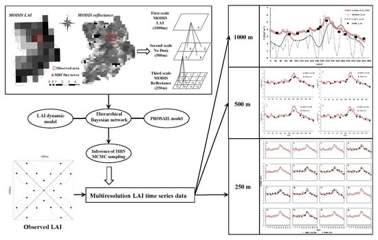
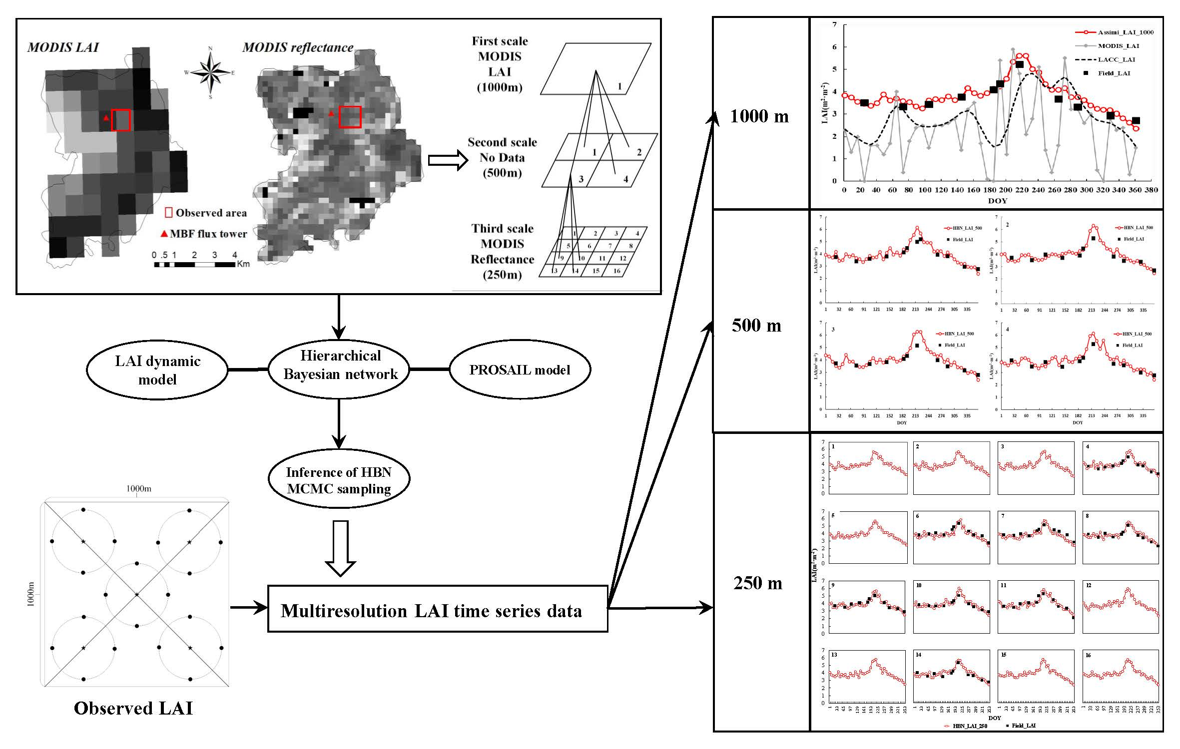
• The 1000-m-resolution MODIS LAI and the 250-m-resolution MODIS reflectance data were processed, which had been carried out in Section 2.2. Smoothed MODIS LAI data were input into the LAI dynamic model to obtain the simulated LAI.
• Based on the 250-m-resolution MODIS reflectance data, resolution-specific likelihood inference (RESL) or resolution-specific restricted-likelihood inference (RESREL) method was used to estimate the parameters in the data assimilation.
• The LAI data and simulated reflectance data at each scale were obtained using the simulated LAI, parameters in the process model of the HBN, and the PROSAIL model. Combined with MODIS reflectance data, the structure of the HBN at three resolutions (1000, 500, and 250 m) was initialized.
• An inference of HBN was used to update node (pixel) states by integrating observations with different spatial resolutions. The probability distributions of node states were updated by upward filtering from observations from the finer scale (250 m) to the coarser scale (1000 m). Then, the downward smoothing started from the coarser scale (1000 m) and ended at the finer scale (250 m) to update the posterior probability distributions of all node states according to all of the observations.
• The Markov chain Monte Carlo (MCMC) sampling method was used to sample the probability distribution. The LAI corresponding to the maximum posterior probability was the assimilation result of the three scales.
• Because of uncertainty and error in the parameter estimation of the HBN, the above process was repeated 100 times and the average value was used as the final assimilation LAI. The assimilated LAI time series data were compared with the observed LAI. The methodology of this HBN algorithm was implemented within MATLAB.

3.1. LAI Dynamic Model

In this study, the semiempirical model developed by Dickinson et al. [57] was used as a dynamic model to obtain the simulated LAI. The model and the parameters suited for MBF have been described previously in the literature [18,20,23]. The model can be expressed as in the following:

$$LA{I}_{t+1}=LA{I}_t+{{\displaystyle \int }}_t^{t+1}\frac{dL}{dt}dt-L_t·LA{I}_t,$$

(1)

$$\frac{dL}{dt}={\lambda }_0·R\left(x\right)·L_0·\left(1-\exp \left(-c·LA{I}_t\right)\right),$$

(2)

$$\frac{dL}{dt}={\lambda }_0·R\left(x\right)·L_0·\left(1-\exp \left(-c·LA{I}_t\right)\right),$$

(3)

$$\mathrm{x}=\left(\mathrm{LAI}-LA{I}_{min}\right)/\left(LA{I}_{max}-LA{I}_{min}\right),$$

(4)

where $LA{I}_{t+1}$ and $LA{I}_t$ represent the LAI at the previous time step ($t+1$) and current time step ($t$), respectively; $R\left(x\right)$ is a smoothing function; $x$ is the normalization of the LAI; $LA{I}_{max}$ and $LA{I}_{min}$ are the maximum and minimum of the LAI in a year, respectively; $L_0$ represents the max LAI; $L_t$ represents the rate of leaf litter; and $L_0$, $L_t$, ${\lambda }_0$, and $c$ are parameters determined based on experience. In this study, the value of $c$ was set as 0.5 and the initial values of the other parameters were obtained according to observed LAI fitting.

3.2. PROSAIL Model

Forest CBR is particularly sensitive to LAI [58]. Therefore, the LAI simulated by the dynamic model was used as the input for the PROSAIL model to achieve simulation of bamboo CBR. The PROSAIL model, which is a combination of the PROSPECT5 and 4SAIL models, is an advanced model for simulation of CBR spectra. The PROSPECT5 model simulates LBR [59], and the 4SAIL model simulates CBR [60]. The parameters of PROSAIL model were optimized using the measured LBR and CBR, and biochemical parameters of the observed area. The optimized parameters are shown in

Table 2. The parameters of PROSAIL model for MBF.

Model	Parameter (Unit)	Value
PROSPECT5	Leaf mesophyll structure $\mathrm{N}$	1.04
	Chlorophyll content $C_{ab}\left(\mathsf{\mu }\mathrm{g}/{\mathrm{cm}}^2\right)$	28–55
	Carotenoids content $C_{ar}\left(\mathsf{\mu }\mathrm{g}/{\mathrm{cm}}^2\right)$	10
	Water content $C_w\left(\mathrm{g}/{\mathrm{cm}}^2\right)$	0.0035
	Dry matter $C_m\left(\mathrm{g}/{\mathrm{cm}}^2\right)$	0.003
4SAIL	Leaf area index $LAI\left({\mathrm{m}}^2/{\mathrm{m}}^2\right)$	0.0–7.0
	Average leaf angle $ALA$ (°)	20.20
	Hot-spot parameter $\mathrm{H}$	0.0003
	View zenith angle ${\theta }_v$ (°)	0–90
	Solar zenith angle ${\theta }_s$ (°)	0–90
	Relative azimuth angle ${\theta }_z$ (°)	0–180

. The reader is referred to the literature for specific details of PROSAIL model and optimization methods [54,59,60,61].

3.3. Hierarchical Bayesian Network Algorithm

In this study, the HBN algorithm was used to obtain LAI time series data with different resolutions for MBF. The algorithm mainly includes the steps of construction of the HBN, inference of the HBN, and MCMC sampling. To simplify the model construction, a transition scale using given data with 500-m resolution was constructed between the MODIS LAI data with 1000-m resolution and MODIS reflectance data with 250-m resolution. This represents a dual relationship between the two datasets on adjacent scales, i.e., one parent node corresponds to four child nodes, as shown in Figure 5.

3.3.1. Construction of the HBN

The HBN include a data model, process model, and parameter model [43,44]. The data, processes, and parameters are defined as three random variables and establish conditional probability distribution models, such that the data assimilation problem is transformed into updating the posterior probability distribution of the processes and parameters under the condition of the existing data [31,45].

1. Data model

The data model defines the conditional probability distribution model between the observed data and real processes, related parameters [46]. In this study, data with three resolutions gradually increasing from top to bottom were included. The first scale considered LAI data with 1000-m resolution, the second scale had no data, and the third scale comprised reflectance data with 250-m resolution. The data model for each scale was defined based on Equations (5)–(7):

$$\mathrm{First}\mathrm{scale}{Z}_{ch\left(i,r\right)}=1Y_{ch\left(i,r\right)}+v_{ch\left(i,r\right)},$$

(5)

$$\mathrm{Second}\mathrm{scale}\hspace{1em}\mathrm{No}\mathrm{data},\mathrm{No}\mathrm{model},$$

(6)

$$\mathrm{Third}\mathrm{scale}{Z}_{ch\left(i,r\right)}=F_{ch\left(i,r\right)}{Y}_{ch\left(i,r\right)}+v_{ch\left(i,r\right)},$$

(7)

where $Z_{ch\left(i,r\right)}$ and $Y_{ch\left(i,r\right)}$ represent the observed data and real process, respectively, for all child nodes of parent node $\left(i,r\right)$, i.e., $Z_{ch\left(i,r\right)}={\left(Z_{c{h}_1\left(i,r\right)},Z_{c{h}_2\left(i,r\right)}\cdots Z_{c{h}_{m_r}\left(i,r\right)}\right)}^{\prime }$ and $Y_{ch\left(i,r\right)}={\left(Y_{c{h}_1\left(i,r\right)},Y_{c{h}_2\left(i,r\right)}\cdots Y_{c{h}_{m_r}\left(i,r\right)}\right)}^{\prime }$; $m_r$ is the number of child nodes at scale $r$; and $v_{ch\left(i,r\right)}$ represents the error of the observed data that obeys a Gaussian distribution $v_{ch\left(i,r\right)}~N\left(0,{\sigma }^2{V}_{ch\left(i,r\right)}\right)$. In this study, at the first scale, $Y$ represents the simulated LAI from the MODIS LAI (MOD15A2) and LAI dynamic model, and $Z$ represents the 1000-m-resolution LAI data with error perturbation. At the third scale, $Y$ represents the LAI with 250-m resolution transmitted from the first scale; the LAI and reflectance data are linked by the PROSAIL model represented by $F_{ch\left(i,r\right)}$, and the simulated reflectance data $Z$ combined with the 250-m-resolution MODIS reflectance data (MOD09Q1) participate in the HBN.

2. Process model

The process model describes the spatiotemporal distribution and variation of parameters, and it defines the conditional dependency between real processes at different scales [46,62]. In this study, the joint posterior probability inference of the real process was transformed into a certain-scale posterior probability inference by defining the conditional dependency between different scales [63]. The process model is defined by Equation (8):

$$Y_{ch\left(i,r\right)}=1Y_{\left(i,r\right)}+w_{ch\left(i,r\right)},$$

(8)

where $Y_{ch\left(i,r\right)}$ represents the real process of node $ch\left(i,r\right)$, which obeys the Gaussian distribution $Y_{ch\left(i,r\right)}~N\left({\mu }_{ch\left(i,r\right)},{\Sigma }_{ch\left(i,r\right)}\right)$; $Y_{\left(i,r\right)}$ is the real process of node $\left(i,r\right)$; and $w_{ch\left(i,r\right)}$ represents the error of the process model that obeys the Gaussian distribution $w_{ch\left(i,r\right)}~N\left(0,{\sigma }^2{W}_{ch\left(i,r\right)}\right)$.

The process model in Equation (8) does not have one-to-one correspondence between $Y_{ch\left(i,r\right)}$ and $\left\{Y_{\left(i,r\right)},w_{ch\left(i,r\right)}\right\}$. Here, $Y_{ch\left(i,r\right)}$ is a vector of length $m_r$, whereas $\left\{Y_{\left(i,r\right)},w_{ch\left(i,r\right)}\right\}$ has a total of $m_r+1$ elements. However, by placing a single linear constraint on the error term $w_{ch\left(i,r\right)}$, a one-to-one correspondence is achieved [64]:

$$q_{\left(i,r\right)}^{\prime }{w}_{ch\left(i,r\right)}=0.$$

(9)

To satisfy Equation (9), we let $Q_{\left(i,r\right)}$ be any $m_r\times \left(m_r-1\right)$ orthonormal matrix with columns that span the space orthogonal to $q_{\left(i,r\right)}$ ($q_{\left(i,r\right)}^{\prime }{Q}_{\left(i,r\right)}=0$ and $Q_{\left(i,r\right)}^{\prime }{Q}_{\left(i,r\right)}=I$). The matrix $Q_{\left(i,r\right)}$ can be taken as the Helmert matrix orthogonal to $q_{ch\left(i,r\right)}$ [65]. Given a $Q_{\left(i,r\right)}$ matrix, any $w_{ch\left(i,r\right)}$ that satisfies Equation (9) can be written as follows:

$$w_{ch\left(i,r\right)}=Q_{\left(i,r\right)}{w}_{\left(i,r\right)}^{\ast },$$

(10)

and then Equation (8) can be written as follows:

$$Y_{ch\left(i,r\right)}=1Y_{\left(i,r\right)}+w_{ch\left(i,r\right)}=1Y_{\left(i,r\right)}+Q_{\left(i,r\right)}{w}_{\left(i,r\right)}^{\ast },$$

(11)

where $w_{\left(i,r\right)}^{\ast }$ obeys the Gaussian distribution $w_{\left(i,r\right)}^{\ast }~N\left(0,{\sigma }^2{W}_{\left(i,r\right)}^{\ast }\right)$, and $W_{ch\left(i,r\right)}=Q_{\left(i,r\right)}{W}_{\left(i,r\right)}^{\ast }{Q}_{\left(i,r\right)}^{\prime }$. By defining $q_{\left(i,r\right)}=a_{ch\left(i,r\right)}=\left(a_{c{h}_1\left(i,r\right)},a_{c{h}_2\left(i,r\right)},\cdots ,a_{c{h}_{m_r}\left(i,r\right)}\right)\prime$, $a_{c{h}_j\left(i,r\right)}$ represents the area of the j-th child of node $\left(i,r\right)$.

3. Parameter model

The parameter model defines the prior distribution of all parameters [32,62]. In this study, the parameters in the data model and the process model included $\sigma$, $V_{ch\left(i,r\right)}$, and $W_{\left(i,r\right)}^{\ast }$. $\sigma$ was a constant, while $V_{ch\left(i,r\right)}$ and $W_{\left(i,r\right)}^{\ast }$ were parameters for Gaussian distribution of $v_{ch\left(i,r\right)}$ in Equations (5), (7) and $w_{\left(i,r\right)}^{\ast }$ in Equation (10). The value of $\sigma$ was set as 10⁻²; the values of $V_{ch\left(i,r\right)}$ in Equations (5) and (7) were calculated by covariance of MODIS LAI and reflectance data, respectively. $W_{\left(i,r\right)}^{\ast }$ was estimated based on $Q_{\left(i,r\right)}$ in Equation (10) using RESL [36] and RESREL [66]; the reader is referred to the literature for specific details [63,64].

3.3.2. Inference of the HBN

The inference of the HBN includes two steps: upward filtering and downward smoothing [67]. For upward filtering, observations information is transmitted from the finer-resolution with 250 m (the bottom scale) to the coarser-resolution with 1000 m (the top scale) to predict and update the probability distribution of nodes using finer-scale observations. Conversely, downward smoothing transmits information from the coarser scale (1000 m) to the finer scale (250 m) to update the posterior probability distributions of all node states according to all of the satellite observations [64,68]. After the above two steps, each node integrates multiple observations with different spatial resolutions, and the final posterior probability distribution is obtained; the reader is referred to the literature for specific details [63].

1. Upward filtering

The initial probability distribution of the data at the top scale is defined as $Y_{\left(i,0\right)}~N\left({\mu }_0,{\Sigma }_0\right)$. Assuming that $\sigma$, $V_{ch\left(i,r\right)}$, and $W_{\left(i,r\right)}^{\ast }$ are known, the probability distribution of all nodes is $Y_{\left(i,r\right)}~N\left({\mu }_{\left(i,r\right)},{\Sigma }_{\left(i,r\right)}\right)$, where the mean ${\mu }_{\left(i,r\right)}$ is the same for all nodes and the variance is ${\Sigma }_{\left(i,r\right)}=W_{\left(i,r\right)}^{\prime }{\Sigma }_{pa\left(i,r\right)}{W}_{\left(i,r\right)}$. The steps of upward filtering are as follows [63]:

Step 1: Calculate the probability distribution of the data at the bottom scale

If there are no observed data at the bottom scale (at the R-1 scale):

$$Y_{\left(i,R-1\right)}|Z_{\left(i,R-1\right)}~N\left({\mu }_{\left(i,R-1\right)},{\Sigma }_{\left(i,R-1\right)}\right).$$

(12)

If there are observed data at the bottom scale (at the R-1 scale):

$$Y_{\left(i,R-1\right)}|Z_{\left(i,R-1\right)}~N\left(m_{\left(i,R-1\right)},{\mathrm{C}}_{\left(i,R-1\right)}\right),$$

(13)

where $Y$ and $Z$ have different meanings at different resolutions and the specific contents are detailed in the data model (as is the same below).

Step 2: Calculate the posterior probability distribution of all nodes

$$Y_{\left(i,r\right)}|Z_{\left(i,r\right)}~N\left(m_{\left(i,r\right)},{\mathrm{C}}_{\left(i,r\right)}\right).$$

(14)

Step 3: Predict probability distribution for parent node $pa\left(i,r\right)$ whose child node is $\left(i,r\right)$

$$Y_{pa\left(i,r\right)}|Z_{pa\left(i,r\right)}^{\ast }~N\left(a_{pa\left(i,r\right)},R_{pa\left(i,r\right)}\right),$$

(15)

where $Z_{pa\left(i,r\right)}^{\ast }$ represents the observation data of the child nodes that do not contain observation data of parent node $pa\left(i,r\right)$.

Step 4: Predict probability distribution of observation of parent node $pa\left(i,r\right)$ whose child node is $\left(i,r\right)$

$$Z_{pa\left(i,r\right)}|Z_{pa\left(i,r\right)}^{\ast }~N\left(f_{pa\left(i,r\right)},{\mathrm{Q}}_{pa\left(i,r\right)}\right),$$

(16)

$$f_{pa\left(i,r\right)}=F_{pa\left(i,r\right)}{a}_{pa\left(i,r\right)},$$

(17)

$${\mathrm{Q}}_{pa\left(i,r\right)}=F_{pa\left(i,r\right)}{R}_{pa\left(i,r\right)}{F}_{pa\left(i,r\right)}^{\prime },$$

(18)

where $F_{pa\left(i,r\right)}$ represents the PROSAIL model and the specific contents are detailed in the data model.

Step 5: Calculate the posterior probability distribution by correcting the prior probability of the observation of parent node $pa\left(i,r\right)$.

Supposing $Y_{pa\left(i,r\right)}|Z_{pa\left(i,r\right)}~N\left(m_{pa\left(i,r\right)},{\mathrm{C}}_{pa\left(i,r\right)}\right)$, then:

If there are no observed data at node $pa\left(i,r\right)$:

$$m_{pa\left(i,r\right)}=f_{pa\left(i,r\right)},$$

(19)

$${\mathrm{C}}_{pa\left(i,r\right)}={\mathrm{Q}}_{pa\left(i,r\right)}.$$

(20)

If there are observed data at node $pa\left(i,r\right)$:

$$m_{pa\left(i,r\right)}=a_{pa\left(i,r\right)}+A_{pa\left(i,r\right)}{e}_{pa\left(i,r\right)},$$

(21)

$${\mathrm{C}}_{pa\left(i,r\right)}=R_{pa\left(i,r\right)}-A_{pa\left(i,r\right)}{Q}_{pa\left(i,r\right)}{A}_{pa\left(i,r\right)}^{\prime },$$

(22)

$$A_{pa\left(i,r\right)}=z_{pa\left(i,r\right)}-f_{pa\left(i,r\right)},$$

(23)

$$e_{pa\left(i,r\right)}=R_{pa\left(i,r\right)}{F}_{pa\left(i,r\right)}^{\prime }{Q}_{pa\left(i,r\right)}^{-1}.$$

(24)

Step 6: Repeat the above steps until at the top scale.

2. Downward smoothing

The posterior probability distribution at the top scale obtained from upward filtering is used as the initial probability distribution for downward smoothing. The steps of downward smoothing are as follows [63]:

Step 1: Obtain the probability distribution of the data at the top scale from upward filtering

$$Y_{\left(i,0\right)}|Z_{\left(i,0\right)}~N\left(s_{\left(i,0\right)},{\mathrm{S}}_{\left(i,0\right)}\right),$$

(25)

where $Y$ and $Z$ have different meanings at different resolutions and the specific contents are detailed in the data model (as is the same below).

Step 2: Calculate the probability distribution of all nodes

$$Y_{\left(i,r\right)}|Z_{\left(i,0\right)}~N\left(s_{\left(i,r\right)},{\mathrm{S}}_{\left(i,r\right)}\right).$$

(26)

Step 3: Calculate the prior probability distribution of any node at any scale

$$Y_{\left(i,r\right)}|Y_{pa\left(i,r\right),}{Z}_{\left(i,r\right)}~N(k_{\left(i,r\right)},K_{\left(i,r\right)},$$

(27)

$$k_{\left(i,r\right)}=K_{\left(i,r\right)}(C_{\left(i,r\right)}^{-1}{m}_{\left(i,r\right)}+W_{\left(i,r\right)}^{-1}1Y_{pa\left(i,r\right),}-{\Sigma }_{\left(i,r\right)}^{-1}{\mu }_{\left(i,r\right)}),$$

(28)

$$K_{\left(i,r\right)}=(C_{\left(i,r\right)}^{-1}+W_{\left(i,r\right)}^{-1}-{\Sigma }_{\left(i,r\right)}^{-1}).$$

(29)

Step 4: Calculate the posterior probability distribution of node $\left(i,r\right)$

$$Y_{\left(i,r\right)}|Z_{\left(i,0\right)}~N\left(s_{\left(i,r\right)},{\mathrm{S}}_{\left(i,r\right)}\right),$$

(30)

$$s_{\left(i,r\right)}=K_{\left(i,r\right)}\left[C_{\left(i,r\right)}^{-1}{m}_{\left(i,r\right)}+W_{\left(i,r\right)}^{-1}1s_{pa\left(i,r\right)}\right],$$

(31)

$${\mathrm{S}}_{\left(i,r\right)}=K_{\left(i,r\right)}+K_{\left(i,r\right)}{W}_{\left(i,r\right)}^{-1}{S}_{pa\left(i,r\right)}{1}^{\prime }{W}_{\left(i,r\right)}^{-1}{K}_{\left(i,r\right)}.$$

(32)

Step 5: Repeat the above steps until at the bottom scale.

3.3.3. MCMC Sampling

After obtaining the posterior probability distribution using the HBN algorithm, a sampling method was used to obtain the LAI value according to the probability distribution [37,41]. Currently, Markov Chain Monte Carlo (MCMC) sampling methods are widely used for such purposes [69,70] and these methods include the Metropolis–Hastings, Gibbs, and Slice sampling [44,71]. In this study, the Metropolis–Hastings method was used to sample the LAI time series data at different scales; the reader is referred to the literature for specific details [72,73,74].

3.4. Accuracy Assessment

The determination coefficient (R²), root mean square error (RMSE), and absolute bias (aBIAS) were used to evaluate the accuracy of the assimilated LAI. Generally, higher values of R² and lower values of both RMSE and aBIAS indicate better accuracy. The RMSE and aBIAS were calculated as follows:

$$\mathrm{RMSE}=\sqrt{\frac{1}{N}{\displaystyle \sum }_{i=1}^N{|y_i-y_0|}_i^2},$$

(33)

$$\mathrm{aBIAS}=\frac{1}{N}{\displaystyle \sum }_{i=1}^N{|y_i-y_0|}_i,$$

(34)

where N indicates the number of samples and it is 11 in this study because of 11 available observed LAI; $y_0$ indicate the values of observed LAI; and $y_i$ represent the values of assimilated LAI.

4. Results and Analysis

4.1. Validation of LAI Assimilation at 1000-m Resolution

The different LAI time series data of MBF at 1000-m resolution are shown in Figure 6. These LAI data include the observed LAI (Field_LAI), original MODIS LAI (MODIS_LAI), smoothed MODIS LAI by LACC (LACC_LAI), and assimilated LAI using the HBN (HBN_LAI_1000) in 2015.

The MODIS_LAI fluctuated considerably (0–6) during the growing season with frequent outliers with low value and errors. Although the LACC_LAI was smoother than MODIS_LAI and the outliers and fluctuations were obviously decreased, it was significantly different from the Field_LAI. The MBF HBN_LAI_1000 showed a trend of slow growth from 3.3 to 4.3 in spring (March–May) before reaching its annual maximum value of 5.6 in summer (June–August). It then decreased gradually from 4.3 to 3.2 in autumn (September–November) with the annual minimum value of 2.3 occurring in winter (December–February). This trend corresponded with the actual trend of MBF LAI. The HBN_LAI_1000 was correlated significantly with the Field_LAI with an R² value of 0.91 and RMSE value of 0.27. However, it was slightly higher than the Field_LAI at DOY 200–320 with a range of overestimation of 0.2–0.4. Analysis of the relationships of both the MODIS_LAI and the HBN_LAI_1000 with the Field_LAI revealed the R² of the HBN_LAI_1000 and Field_LAI was 2.7 times higher and the RMSE was 87.8% lower compared with the MODIS_LAI and Field_LAI. This indicates the assimilated LAI obtained by the HBN algorithm greatly improves the accuracy and reduces the error of the MODIS_LAI, producing better correspondence with the actual LAI data. Thus, the HBN_LAI_1000 can reflect the dynamic changes of MBF LAI over a long time series.

4.2. Validation of LAI Assimilation at 500-m Resolution

The time series data of observed LAI (Field_LAI) and assimilated LAI (HBN_LAI_500) of MBF at 500-m resolution in 2015 are shown in Figure 7. Traces 1–4 are the LAI assimilation results of the four pixels with 500-m resolution that correspond to one pixel at 1000-m resolution.

The HBN_LAI_500 of the four pixels showed a trend of growth in spring (3.3–4.1, 3.5–4.0, 3.4–4.2, 3.3–4.2) before reaching maximum values in summer (6.1, 6.3, 6.3, 6.1), decreasing in autumn (4.9–3.2, 4.5–3.2, 4.6–3.2, 4.5–3.2), and reaching minimum values in winter (2.4, 2.5, 2.4, 2.4). This trend, which corresponded with the actual trend of LAI, was consistent with the HBN_LAI_1000 in MBF; however, compared with the HBN_LAI_1000, more fluctuations were evident in the HBN_LAI_500. The HBN_LAI_500 of the four pixels correlated significantly with the Field_LAI; the R² values for pixels 1–4 were 0.89, 0.90, 0.93, and 0.87, respectively with RMSE values of < 0.50 and aBIAS values of < 0.40. However, the HBN_LAI_500 was obviously overestimated in comparison with the Field_LAI during the growing period (DOY 200–250) with overestimations of 1.2, 1.0, 1.1, and 0.8 for pixels 1–4, respectively, similar to the HBN_LAI_1000. Although the accuracy of the MBF HBN_LAI_500 is shown slightly lower than the HBN_LAI_1000, it still has reasonably high accuracy and it corresponds with the actual LAI data.

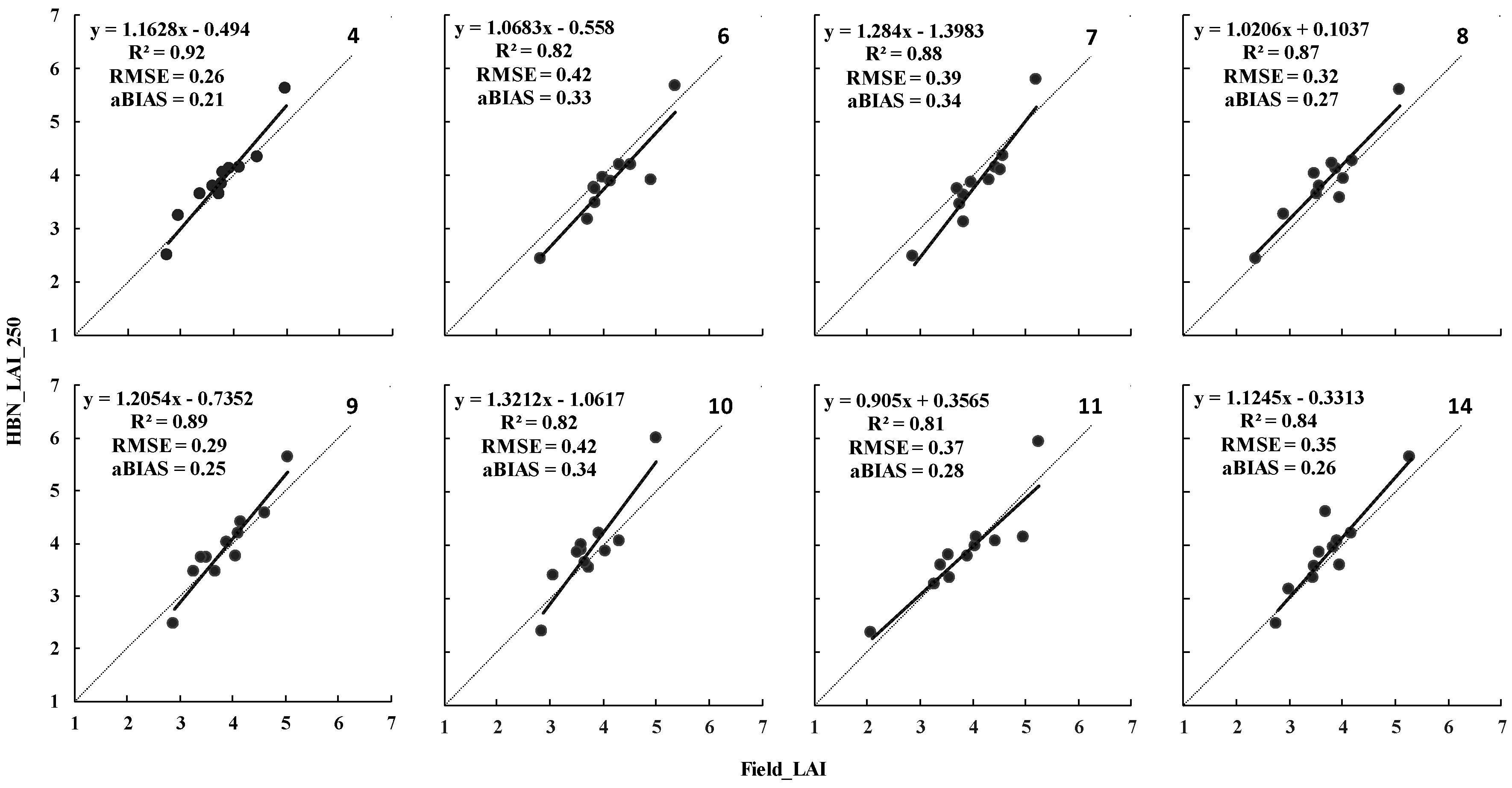
4.3. Validation of LAI Assimilation at 250-m Resolution

The time series data of observed LAI (Field_LAI) and assimilated LAI (HBN_LAI_250) of MBF at 250-m resolution in 2015, and the correlations between them, are shown in Figure 8 and Figure 9. Traces 1–16 are the LAI assimilation results of the 16 pixels with 250-m resolution that correspond to one pixel at 1000-m resolution.

The HBN_LAI_250 of the 16 pixels was consistent with the actual trend of LAI, although considerable fluctuation was evident, especially at DOY 0–200. During the growing period in summer (DOY 200–250), the HBN_LAI_250 of eight pixels (4, 6, 7, 8, 9, 10, 11, and 14) were obviously overestimated in comparison with the Field_LAI with a range of overestimation of 0.4–1.0. For the HBN_LAI_250 and Field_LAI (Figure 9), the R² values were >0.80 (the R² value for the fourth pixel was 0.92), RMSE values were <0.50, and aBIAS values were <0.40. This indicates that the HBN_LAI_250 for MBF has high accuracy and it is an effective assimilation result of multiresolution LAI using HBN algorithm.

5. Discussion and Conclusions

Several researches had achieved the acquisition of multiresolution LAI using multiresolution tree combined with a Kalman filter [28,29], and had validated the precision comparing with high-resolution LAI [30]. This study developed an HBN algorithm coupled with a LAI dynamic model and the PROSAIL model to assimilate LAI data with different resolutions (1000, 500, and 250 m) of MBF. The results showed that the multiresolution HBN_LAI corresponded with the actual trend of growth of the MBF and that it was correlated significantly with the Field_LAI (R² values reached >0.80). The R² value between the HBN_LAI and Field_LAI at 1000-m resolution was 0.91 and the RMSE value was 0.27; at 500-m resolution, the averages of the R² values and the RMSE values were 0.90 and 0.42; and at 250-m resolution, the averages of the R² values and the RMSE values were 0.86 and 0.35. The HBN_LAI at the coarsest scale (1000-m resolution) provided better accuracy, which was consistent with the finding in literature [30]. Compared with the MODIS_LAI, the R² value of the HBN_LAI_1000 increased by 2.7 times, while the RMSE value decreased by 87.8%. Compared with other researches on improving the precision of MODIS LAI products [7,18,23], this study had achieved better results. Therefore, the HBN algorithm significantly improved the accuracy and reduced the error of the MODIS LAI products, and accurate LAI at different scales could be obtained.

Analysis of the results revealed that the HBN_LAI_1000, HBN_LAI_500, and HBN_LAI_250 obviously overestimated with 7.5%, 20.0%, and 11.3%, respectively, at DOY 217. This overestimation can be explained in terms of the following three aspects.

First, differences between MODIS reflectance and the reflectance simulated by the PROSAIL model will affect the assimilation results [18,22]. As there are no MODIS reflectance data available at 1000- and 500-m resolution, the reflectance at 1000- and 500-m resolution is transmitted from the MODIS reflectance at the bottom scale of 250-m resolution, which is different from the simulated reflectance. This will have an impact on the HBN_LAI_1000 and HBN_LAI_500 and overestimation will occur. At 250-m resolution, the difference between MODIS reflectance and simulated reflectance transmitted by the process model has an influence on the HBN_LAI_250. Figure 10 shows the RED and NIR bands of MODIS reflectance and simulated reflectance of 16 pixels at 250-m resolution. The MODIS reflectance data of the 16 pixels has considerable fluctuation and some outliers (hollow circles in Figure 10), while the reflectance simulated by the PROSAIL model is more concentrated and has less fluctuation than MODIS reflectance. In the RED band, the mean value of MODIS reflectance is higher than the simulated reflectance. The maximum MODIS reflectance is up to 1.7 times that of the simulated reflectance. In contrast, in the NIR band, the mean value of simulated reflectance is higher than MODIS reflectance. The minimum MODIS reflectance is 67% of the simulated reflectance. In the hierarchical Bayesian inference, the LAI with 500- and 250-m resolution is inferred from the 1000-m-resolution LAI and the parameter $w_{ch\left(i,r\right)}$ in process model, causing an overestimation of LAI at the 500- and 250-m scale. Furthermore, there is considerable difference between the simulated reflectance and MODIS reflectance, and the HBN_LAI_250 is overestimated. Yang et al. [75], Li et al. [18] and Li et al. [22] have all highlighted that error between the simulated reflectance and MODIS reflectance is one of the primary reasons for inaccuracy in LAI estimations.

Second, the uncertainty of the estimated parameter $w_{ch\left(i,r\right)}$ in the process model will also cause errors in the assimilation results. In the HBN algorithm, RESL and RESREL used to estimate parameter $W_{\left(i,r\right)}^{\ast }$ by using MODIS reflectance data, and then parameter $w_{ch\left(i,r\right)}$ was obtained using Equation (6). In the hierarchical Bayesian inference, the LAI with 500- and 250-m resolution is inferred from the 1000-m-resolution LAI and parameter $w_{ch\left(i,r\right)}$ in the process model, uncertainty in the estimated parameter $w_{ch\left(i,r\right)}$ causes errors of LAI at 500- and 250-m resolution, which in turn affects the assimilation results. In this study, 100 iterations of the HBN were performed to reduce the errors. Figure 11 shows the mean value and standard deviation (SD) of parameter $w_{ch\left(i,r\right)}$ for MBF at the 1000–500-m and 500–250-m scales, respectively. The mean value of $w_{ch\left(i,r\right)}$ is maintained between −0.10 and 0.10 at the 1000–500-m scale, except for some nodes with outliers. However, at DOY 230–290, $w_{ch\left(i,r\right)}$ is slightly larger than that at other periods, and the SD of $w_{ch\left(i,r\right)}$ is very large, indicating that the uncertainty is substantial during this period. The SD for the first, second, and third child node is 6, 5, and 10 times greater, respectively, than the mean value. At the 500–250-m scale, considerable fluctuations are evident in both $w_{ch\left(i,r\right)}$ and its SD and the mean value of $w_{ch\left(i,r\right)}$ is maintained between −0.20 and 0.20. Similar to the 1000–500-m scale, $w_{ch\left(i,r\right)}$ at DOY 230–290 is larger than that at other periods with greater uncertainty, which could be related to the overestimation of the HBN_LAI for MBF at DOY 217.

Finally, the overestimation of the HBN_LAI_500 for MBF is most serious because of the lack of original observation data at 500-m resolution. The inference of the HBN and update of the LAI posterior probability at 500-m scale rely on MODIS LAI products with 1000-m resolution and MODIS reflectance data with 250-m resolution, in which the bidirectional accumulation of errors is unavoidable. Therefore, overestimation is more serious in the HBN_LAI_500. To avoid this phenomenon, the application of multisource remote sensing data, e.g., Landsat data, could be considered to provide multiresolution data for the HBN assimilation. Moreover, the complex structure could be taken into account to flexibly adjust the relationship between parent–child nodes in the HBN and to describe irregular shapes of geographical regions [30].

In this study, the HBN algorithm was developed to obtain high precision LAI time series data from MODIS data at different spatial resolutions (1000, 500, and 250 m). The results demonstrated that the assimilated LAI values at each spatial resolution were in good agreement with the actual trend of MBF LAI and the assimilated LAI at the coarsest scale (1000 m) provided best accuracy. The accuracy of assimilated LAI was significantly improved compared with MODIS LAI products. Therefore, the HBN algorithm applied in this study can effectively obtain highly accurate multiresolution LAI time series data for bamboo forest. This study achieved multiresolution LAI time series data using HBN algorithm at MBF flux measurement site. In the near future, we will extend the methodology to obtain multiscale LAI data on the regional scale.

References

1. Chen, J.; Black, T.A. Defining leaf area index for non-flat leaves. Plant Cell Environ. 1992, 15, 421–429. [Google Scholar] [CrossRef]
2. Sellers, P.J.; Dickinson, R.E.; Randall, D.A.; Betts, A.K.; Hall, F.G.; Berry, J.A.; Collatz, G.J.; Denning, A.S.; Mooney, H.A.; Nobre, C.A. Modeling the Exchanges of Energy, Water, and Carbon between Continents and the Atmosphere. Science 1997, 275, 502–509. [Google Scholar] [CrossRef] [PubMed]
3. Pasolli, L.; Asam, S.; Castelli, M.; Bruzzone, L.; Wohlfahrt, G.; Zebisch, M.; Notarnicola, C. Retrieval of Leaf Area Index in mountain grasslands in the Alps from MODIS satellite imagery. Remote Sens. Environ. 2015, 165, 159–174. [Google Scholar] [CrossRef]
4. Kauwe, M.G.D.; Disney, M.I.; Quaife, T.; Lewis, P.; Williams, M. An assessment of the MODIS collection 5 leaf area index product for a region of mixed coniferous forest. Remote Sens. Environ. 2011, 115, 767–780. [Google Scholar] [CrossRef]
5. Jonckheere, I.; Fleck, S.; Nackaerts, K.; Muys, B.; Coppin, P.; Weiss, M.; Baret, F. Review of methods for in situ leaf area index determination: Part I. Theories, sensors and hemispherical photography. Agric. For. Meteorol. 2004, 121, 19–35. [Google Scholar] [CrossRef]
6. Dong, T.; Liu, J.; Qian, B.; Zhao, T.; Jing, Q.; Geng, X.; Wang, J.; Huffman, T.; Shang, J. Estimating winter wheat biomass by assimilating leaf area index derived from fusion of Landsat-8 and MODIS data. Int. J. Appl. Earth Obs. Geoinf. 2016, 49, 63–74. [Google Scholar] [CrossRef]
7. Li, X.; Xiao, Z.; Wang, J.; Ying, Q.U.; Jin, H. Dual Ensemble Kalman Filter assimilation method for estimating time series LAI. J. Remote Sens. 2014, 18, 27–44. [Google Scholar] [CrossRef]
8. Gray, J.; Song, C. Mapping leaf area index using spatial, spectral, and temporal information from multiple sensors. Remote Sens. Environ. 2012, 119, 173–183. [Google Scholar] [CrossRef]
9. Myneni, R.B.; Hoffman, S.; Knyazikhin, Y.; Privette, J.L.; Glassy, J.; Tian, Y.; Wang, Y.; Song, X.; Zhang, Y.; Smith, G.R. Global products of vegetation leaf area and fraction absorbed PAR from year one of MODIS data. Remote Sens. Environ. 2002, 83, 214–231. [Google Scholar] [CrossRef] [Green Version]
10. Baret, F.; Hagolle, O.; Geiger, B.; Bicheron, P.; Miras, B.; Huc, M.; Berthelot, B.; Niño, F.; Weiss, M.; Samain, O. LAI, fAPAR and fCover CYCLOPES global products derived from VEGETATION: Part 1: Principles of the algorithm. Remote Sens. Environ. 2007, 110, 275–286. [Google Scholar] [CrossRef]
11. Deng, F.; Chen, J.M.; Plummer, S.; Chen, M.; Pisek, J. Algorithm for global leaf area index retrieval using satellite imagery. IEEE Trans. Geosci. Remote Sens. 2006, 44, 2219–2229. [Google Scholar] [CrossRef] [Green Version]
12. Masson, V.; Champeaux, J.L.; Chauvin, F.; Meriguet, C.; Lacaze, R. A Global Database of Land Surface Parameters at 1-km Resolution in Meteorological and Climate Models. J. Clim. 2003, 16, 1231–1281. [Google Scholar] [CrossRef]
13. Gao, F.; Morisette, J.T.; Wolfe, R.E.; Ederer, G.; Pedelty, J.; Masuoka, E.; Myneni, R.; Tan, B.; Nightingale, J. An Algorithm to Produce Temporally and Spatially Continuous MODIS-LAI Time Series. IEEE Geosci. Remote Sens. Lett. 2008, 5, 60–64. [Google Scholar] [CrossRef]
14. Fang, H.; Liang, S.; Townshend, J.R.; Dickinson, R.E. Spatially and temporally continuous LAI data sets based on an integrated filtering method: Examples from North America. Remote Sens. Environ. 2013, 112, 75–93. [Google Scholar] [CrossRef]
15. Borak, J.S.; Jasinski, M.F. Effective interpolation of incomplete satellite-derived leaf-area index time series for the continental United States. Agric. For. Meteorol. 2008, 149, 320–332. [Google Scholar] [CrossRef]
16. Ma, J.; Qin, S. Recent Advances and Development of Data Assimilation Algorithms. Adv. Earth Sci. 2012, 27, 747–757. [Google Scholar] [CrossRef]
17. Mclaughlin, D.; Miller, C.T.; Parlange, M.B.; Hassanizadeh, S.M. An integrated approach to hydrologic data assimilation: Interpolation, smoothing, and filtering. Adv. Water Resour. 2002, 25, 1275–1286. [Google Scholar] [CrossRef]
18. Li, X.; Mao, F.; Du, H.; Zhou, G.; Xu, X.; Han, N.; Sun, S.; Gao, G.; Chen, L. Assimilating leaf area index of three typical types of subtropical forest in China from MODIS time series data based on the integrated ensemble Kalman filter and PROSAIL model. ISPRS J. Photogramm. Remote Sens. 2017, 126, 68–78. [Google Scholar] [CrossRef]
19. Zhao, Y.; Chen, S.; Shen, S. Assimilating remote sensing information with crop model using Ensemble Kalman Filter for improving LAI monitoring and yield estimation. Ecol. Model. 2013, 270, 30–42. [Google Scholar] [CrossRef]
20. Mao, F.; Li, X.; Du, H.; Zhou, G.; Han, N.; Xu, X.; Liu, Y.; Chen, L.; Cui, L. Comparison of Two Data Assimilation Methods for Improving MODIS LAI Time Series for Bamboo Forests. Remote Sens. 2017, 9, 401. [Google Scholar] [CrossRef]
21. Li, H.; Chen, Z.; Wu, W.; Jiang, Z.; Liu, B.; Hasi, T. Crop model data assimilation with particle filter for yield prediction using leaf area index of different temporal scales. In Proceedings of the Fourth International Conference on Agro-Geoinformatics, Istanbul, Turkey, 20–24 July 2015; pp. 401–406. [Google Scholar]
22. Li, X.; Du, H.; Mao, F.; Zhou, G.; Chen, L.; Xing, L.; Fan, W.; Xu, X.; Liu, Y.; Cui, L. Estimating bamboo forest aboveground biomass using EnKF-assimilated MODIS LAI spatiotemporal data and machine learning algorithms. Agric. For. Meteorol. 2018, 256–257, 445–457. [Google Scholar] [CrossRef]
23. Li, X.; Mao, F.; Du, H.; Zhou, G.; Xu, X.; Li, P.; Liu, Y.; Cui, L. Simulating of carbon fluxes in bamboo forest ecosystem using BEPS model based on the LAI assimilated with Dual Ensemble Kalman Filter. Chin. J. Appl. Ecol. 2016. [Google Scholar] [CrossRef]
24. Li, X.; Lu, H.; Yu, L.; Yang, K. Comparison of the Spatial Characteristics of Four Remotely Sensed Leaf Area Index Products over China: Direct Validation and Relative Uncertainties. Remote Sens. 2018, 10, 148. [Google Scholar] [CrossRef]
25. Yuan, H.; Dai, Y.; Xiao, Z.; Ji, D.; Shangguan, W. Reprocessing the MODIS Leaf Area Index products for land surface and climate modelling. Remote Sens. Environ. 2011, 115, 1171–1187. [Google Scholar] [CrossRef]
26. Jinsheng, H. Carbon cycling of Chinese forests: From carbon storage, dynamics to models. Sci. China Life Sci. 2012, 55, 188–190. [Google Scholar] [CrossRef] [Green Version]
27. Cao, M.; Yu, G.; Liu, J.; Li, K. Multi-scale observation and cross-scale mechanistic modeling on terrestrial ecosystem carbon cycle. Sci. China 2005, 48, 17–32. [Google Scholar] [CrossRef]
28. Xiao, Z.; Wang, J.; Wan, H. Multiscale approach for fusing leaf area index estimates from multiple sensors. Proc. SPIE 2007, 6790, 679013. [Google Scholar] [CrossRef]
29. Wang, D.; Liang, S. Using multiresolution tree to integrate MODIS and MISR-L3 LAI products. In Proceedings of the IEEE International Geoscience & Remote Sensing Symposium, Honolulu, HI, USA, 25–30 July 2010; Volume 38, pp. 1027–1030. [Google Scholar] [CrossRef]
30. Jiang, J.; Xiao, Z.; Wang, J.; Song, J. Multiscale Estimation of Leaf Area Index from Satellite Observations Based on an Ensemble Multiscale Filter. Remote Sens. 2016, 8, 229. [Google Scholar] [CrossRef]
31. Smith, A.F.M.; Berliner, L.M.; Royle, J.A.; Wikle, C.K.; Milliff, R.F. Bayesian Methods in the Atmospheric Sciences; Oxford University Press: Oxford, UK, 1998. [Google Scholar]
32. Wikle, C.K.; Anderson, C.J. Climatological analysis of tornado report counts using a hierarchical Bayesian spatiotemporal model. J. Geophys. Res. Atmos. 2003, 108. [Google Scholar] [CrossRef] [Green Version]
33. Wikle, C.K.; Berliner, L.M.; Cressie, N. Hierarchical Bayesian space-time models. Environ. Ecol. Stat. 1998, 5, 117–154. [Google Scholar] [CrossRef]
34. Berliner, L.M. Hierarchical Bayesian Time Series Models; Springer: Dordrecht, The Netherlands, 1996; pp. 15–22. [Google Scholar]
35. Wikle, C.K.; Berliner, M.L. Combining Information Across Spatial Scales. Technometrics 2005, 47, 80–91. [Google Scholar] [CrossRef]
36. Kolaczyk, E.D.; Huang, H. Multiscale Statistical Models for Hierarchical Spatial Aggregation. Geogr. Anal. 2010, 33, 95–118. [Google Scholar] [CrossRef] [Green Version]
37. Berrocal, V.J.; Gelfand, A.E.; Holland, D.M. A Spatio-Temporal Downscaler for Output From Numerical Models. J. Agric. Biol. Environ. Stat. 2010, 15, 176–197. [Google Scholar] [CrossRef] [PubMed] [Green Version]
38. Sahu, S.K.; Yip, S.; Holland, D.M. Improved space–time forecasting of next day ozone concentrations in the eastern US. Atmos. Environ. 2009, 43, 494–501. [Google Scholar] [CrossRef]
39. Sahu, S.K.; Gelfand, A.E.; Holland, D.M. High Resolution Space-Time Ozone Modeling for Assessing Trends. J. Am. Stat. Assoc. 2007, 102, 1221. [Google Scholar] [CrossRef] [PubMed]
40. Berliner, L.M.; Milliff, R.F.; Wikle, C.K. Bayesian hierarchical modeling of air-sea interaction. J. Geophys. Res. Oceans 2003, 108, 303–307. [Google Scholar] [CrossRef]
41. Mcmillan, N.J.; Holland, D.M.; Morara, M.; Feng, J. Combining numerical model output and particulate data using Bayesian space-time modeling. Environmetrics 2010, 21, 48–65. [Google Scholar] [CrossRef]
42. Fuentes, M.; Raftery, A.E. Model evaluation and spatial interpolation by Bayesian combination of observations with outputs from numerical models. Biometrics 2005, 61, 36. [Google Scholar] [CrossRef]
43. Cocchi, D.; Greco, F.; Trivisano, C. Hierarchical space-time modelling of PM pollution. Atmos. Environ. 2007, 41, 532–542. [Google Scholar] [CrossRef]
44. Gelfand, A.E.; Sahu, S.K. Combining monitoring data and computer model output in assessing environmental exposure. In Oxford Handbook of Applied Bayesian Analysis; Oxford University Press: Oxford, UK, 2010; pp. 482–510. [Google Scholar]
45. Qin, S.; Ma, J.; Wang, X. Construction and Experiment of Hierarchical Bayesian Network in Data Assimilation. IEEE J. Sel. Top. Appl. Earth Obs. Remote Sens. 2013, 6, 1036–1047. [Google Scholar] [CrossRef]
46. Qin, S.; Ma, J.; Wang, X. Development of a hierarchical Bayesian network algorithm for land surface data assimilation. Int. J. Remote Sens. 2013, 34, 1905–1927. [Google Scholar] [CrossRef]
47. Du, H.; Zhou, G.; Xu, X. Quantitative Methods Using Remote Sensing in Estimating Biomass and Carbon Storage Bamboo Forest; Science Press: Beijing, China, 2012. [Google Scholar]
48. Zhou, G.; Jiang, P.; Du, H.; Shi, Y. Technology for the Measurement and Enhancement Carbon Sinks in Bamboo Forest Ecosystems; Science Press: Beijing, China, 2017. [Google Scholar]
49. Han, N.; Du, H.; Zhou, G.; Xu, X.; Cui, R.; Gu, C. Spatiotemporal heterogeneity of Moso bamboo aboveground carbon storage with Landsat Thematic Mapper images: A case study from Anji County, China. Int. J. Remote Sens. 2013, 34, 4917–4932. [Google Scholar] [CrossRef]
50. Du, H.; Zhou, G.; Ge, H.; Fan, W.; Xu, X.; Fan, W.; Shi, Y. Satellite-based carbon stock estimation for bamboo forest with a non-linear partial least square regression technique. Int. J. Remote Sens. 2012, 33, 1917–1933. [Google Scholar] [CrossRef]
51. Zhou, G.; Xu, X.; Du, H.; Ge, H.; Shi, Y.; Zhou, Y. Estimating Aboveground Carbon of Moso Bamboo Forests Using the k Nearest Neighbors Technique and Satellite Imagery. Photogramm. Eng. Remote Sens. 2011, 77, 1123–1131. [Google Scholar] [CrossRef]
52. Chen, J.M.; Deng, F.; Chen, M. Locally adjusted cubic-spline capping for reconstructing seasonal trajectories of a satellite-derived surface parameter. IEEE Trans. Geosci. Remote Sens. 2006, 44, 2230–2238. [Google Scholar] [CrossRef]
53. Xiao, Z.; Liang, S.; Wang, J.; Jiang, B.; Li, X. Real-time retrieval of Leaf Area Index from MODIS time series data. Remote Sens. Environ. 2011, 115, 97–106. [Google Scholar] [CrossRef]
54. Li, X. Assimilation of MODIS LAI Time Series in Bamboo Forest and Its Application in Carbon Flux Simulation; Zhejiang A&F University: Hangzhou, China, 2017. [Google Scholar]
55. Sun, S.; Du, H.; Li, P.; Zhou, G.; Xu, X.; Gao, G.; Li, X. Retrieval of leaf net photosynthetic rate of moso bamboo forests using hyperspectral remote sen-sing based on wavelet transform. Chin. J. Appl. Ecol. 2016, 27, 49–58. [Google Scholar] [CrossRef]
56. Lu, G.; Du, H.; Zhou, G.; Lv, Y.; Gu, C.; Shang, Z. Dynamic change of Phyllostachys edulis forest canopy parameters and their relationships with photosynthetic active radiation in the bamboo shooting growth phase. J. Zhejiang A F Univ. 2012, 29, 844–850. [Google Scholar] [CrossRef]
57. Dickinson, R.E.; Tian, Y.; Liu, Q.; Zhou, L. Dynamics of leaf area for climate and weather models. J. Geophys. Res. Atmos. 2008, 113. [Google Scholar] [CrossRef] [Green Version]
58. Jacquemoud, S.; Verhoef, W.; Baret, F.; Bacour, C.; Zarcotejada, P.J.; Asner, G.P.; François, C.; Ustin, S.L.; Ustin, S.L.; Schaepman, M.E. PROSPECT+SAIL models: A review of use for vegetation characterization. Remote Sens. Environ. 2009, 113, S56–S66. [Google Scholar] [CrossRef]
59. Feret, J.B.; François, C.; Asner, G.P.; Gitelson, A.A.; Martin, R.E.; Bidel, L.P.R.; Ustin, S.L.; Maire, G.L.; Jacquemoud, S. PROSPECT-4 and 5: Advances in the leaf optical properties model separating photosynthetic pigments. Remote Sens. Environ. 2008, 112, 3030–3043. [Google Scholar] [CrossRef]
60. Verhoef, W.; Bach, H. Coupled soil–leaf-canopy and atmosphere radiative transfer modeling to simulate hyperspectral multi-angular surface reflectance and TOA radiance data. Remote Sens. Environ. 2007, 109, 166–182. [Google Scholar] [CrossRef]
61. Gu, C.; Du, H.; Zhou, G.; Han, N.; Xu, X.; Zhao, X.; Sun, X. Retrieval of leaf area index of moso bamboo forest with Landsat Thematic Mapper image based on PROSAIL canopy radiative transfer model. Chin. J. Appl. Ecol. 2013, 24, 2248–2256. [Google Scholar] [CrossRef]
62. Wikle, C.K.; Berliner, L.M. A Bayesian tutorial for data assimilation. Phys. D Nonlinear Phenom. 2007, 230, 1–16. [Google Scholar] [CrossRef]
63. Ma, J. Data Assimilation Algorithm Development and Experiment; Science Press: Beijing, China, 2013. [Google Scholar]
64. Gybels, J.; Martin, P. Multi-Resolution Statistical Modeling in Space and Time with Application to Remote Sensing of the Environment; Ohio State University: Columbus, OH, USA, 2003. [Google Scholar]
65. Harville, D.A. Matrix Algebra From a Statistician’s Perspective; Springer: New York, NY, USA, 1997. [Google Scholar]
66. Mcculloch, C.E.; Searle, S.R. Generalized, Linear, and Mixed Models; Wiley: Hoboken, NJ, USA, 2008. [Google Scholar]
67. Ferreira, M.A.R.; Lee, H.K.H. Multiscale Modeling: A Bayesian Perspective; Springer: Berlin/Heidelberg, Germany, 2007. [Google Scholar]
68. Huang, H.C.; Cressie, N.; Gabrosek, J. Fast, Resolution-Consistent Spatial Prediction of Global Processes From Satellite Data. J. Comput. Graph. Stat. 2002. [Google Scholar] [CrossRef]
69. Geweke, J. Bayesian Inference in Econometric Models Using Monte Carlo Integration. Econometrica 1989, 57, 1317–1339. [Google Scholar] [CrossRef]
70. Hastings, W.K. Monte Carlo Sampling Methods Using Markov Chains and Their Applications. Biometrika 1970, 57, 97–109. [Google Scholar] [CrossRef]
71. Smith, A.F.M.; Roberts, G.O. Bayesian Computation Via the Gibbs Sampler and Related Markov Chain Monte Carlo Methods. J. R. Stat. Soc. 1993, 55, 3–23. [Google Scholar] [CrossRef]
72. Flötteröd, G.; Bierlaire, M. Metropolis–Hastings sampling of paths. Transp. Res. Part B 2013, 48, 53–66. [Google Scholar] [CrossRef]
73. Geweke, J.; Tanizaki, H. Bayesian estimation of state-space models using the Metropolis–Hastings algorithm within Gibbs sampling. Comput. Stat. Data Anal. 2001, 37, 151–170. [Google Scholar] [CrossRef] [Green Version]
74. Chib, S.; Greenberg, E. Understanding the Metropolis-Hastings Algorithm. Am. Stat. 1995, 49, 327–335. [Google Scholar] [CrossRef] [Green Version]
75. Yang, W.; Tan, B.; Huang, D.; Rautiainen, M.; Shabanov, N.V.; Wang, Y.; Privette, J.L.; Huemmrich, K.F.; Fensholt, R.; Sandholt, I. MODIS leaf area index products: From validation to algorithm improvement. IEEE Trans. Geosci. Remote Sens. 2006, 44, 1885–1898. [Google Scholar] [CrossRef]
Figure 1. (a) Anji county in northwest Zhejiang province and land use types; (b) Shanchuan town in southeast Anji county and Moso bamboo forest distribution; (c) MODIS LAI product for the Shanchuan town at DOY 225 in 2015 and spatial location of MBF flux measurement site and observed area.
Remotesensing 11 00056 g001
Figure 2. NDVI time series envelope and outliers.
Remotesensing 11 00056 g002
Figure 3. (a) Image of MBF using digital camera with fisheye lens; and (b) analysis of corresponding LAI using LAI (2000G)-LogCI algorithm in the WinSCANOPY v2009a program.
Remotesensing 11 00056 g003
Figure 4. Plot design of observed LAI in observed area of 1 × 1 km (Stars represent observation center, and dots indicate observation points).
Remotesensing 11 00056 g004
Figure 5. Flow chart of process for estimation of LAI using the hierarchical Bayesian network (HBN) algorithm with multiresolution data (LACC respects locally adjusted cubic-spline capping for processing of MODIS LAI; SG respects Savitzky-Golay smooth for processing of MODIS reflectance; MCMC means Markov Chain Monte Carlo sampling method; HBN_LAI_1000, HBN_LAI_500, and HBN_LAI_250 indicate the assimilated LAI by using HBN algorithm at 1000 m, 500 m, and 250 m resolution, respectively; and Field_LAI_1000, Field_LAI_500, and Field_LAI_250 indicate observed LAI at 1000 m, 500 m, and 250 m resolution, respectively).
Remotesensing 11 00056 g005
Figure 6. Time series of Field_LAI, MODIS_LAI, LACC_LAI, and HBN_LAI_1000 of MBF at 1000-m resolution in 2015; and comparison between Field_LAI and MODIS_LAI, HBN_LAI_1000 (The number of samples (N) is 11).
Remotesensing 11 00056 g006
Figure 7. Time series of Field_LAI and HBN_LAI_500 for four pixels of MBF at 500-m resolution in 2015; and comparison between Field_LAI and HBN_LAI_500 of four pixels (N = 11).
Remotesensing 11 00056 g007
Figure 8. Time series of Field_LAI and HBN_LAI_250 for sixteen pixels of MBF at 250-m resolution in 2015.
Remotesensing 11 00056 g008
Figure 9. Comparison between the Field_LAI and HBN_LAI_250 of eight pixels (N = 11).
Remotesensing 11 00056 g009
Figure 10. Comparison of MODIS reflectance and canopy reflectance simulated by the PROSAIL model for MBF (The boxplot represents the statistical characteristics of MODIS reflectance; the dot indicates the average of a certain pixel and the hollow circle indicates outlier for the entire year. The red line represents the average reflectance simulated by the PROSAIL model and the region colored light red is the interval of simulated reflectance).
Remotesensing 11 00056 g010
Figure 11. Mean value and uncertainty of w c h ( i , r ) of the process model for MBF.
Remotesensing 11 00056 g011