Assessing the Potential Benefits of the Geostationary Vantage Point for Generating Daily Chlorophyll-a Maps in the Baltic Sea

Abstract

Currently, observations from low-Earth orbit (LEO) ocean color sensors represent one of the most used tools to study surface optical and biogeochemical properties of the ocean. LEO observations are available at daily temporal resolution, and are often combined into weekly, monthly, seasonal, and annual averages in order to obtain sufficient spatial coverage. Indeed, daily satellite maps of the main oceanic variables (e.g., surface phytoplankton chlorophyll-a) generally have many data gaps, mainly due to clouds, which can be filled using either Optimal Interpolation or the Empirical Orthogonal Functions approach. Such interpolations, however, may introduce large uncertainties in the final product. Here, our goal is to quantify the potential benefits of having high-temporal resolution observations from a geostationary (GEO) ocean color sensor to reduce interpolation errors in the reconstructed hourly and daily chlorophyll-a products. To this aim, we used modeled chlorophyll-a fields from the Copernicus Marine Environment Monitoring Service’s (CMEMS) Baltic Monitoring and Forecasting Centre (BAL MFC) and satellite cloud observations from the Spinning Enhanced Visible and Infrared Imager (SEVIRI) sensor (on board the geostationary satellite METEOSAT). The sampling of a GEO was thus simulated by combining the hourly chlorophyll fields and clouds masks, then hourly and daily chlorophyll-a products were generated after interpolation from neighboring valid data using the Multi-Channel Singular Spectral Analysis (M-SSA). Two cases are discussed: (i) A reconstruction based on the typical sampling of a LEO and, (ii) a simulation of a GEO sampling with hourly observations. The results show that the root mean square and interpolation bias errors are significantly reduced using hourly observations.

1. Introduction

Currently, accurate knowledge of biogeochemical parameters is extremely important for many marine environmental applications. Indeed, these variables are generally used to describe the evolution of marine ecosystems in relation to climate change [1,2]. An essential parameter, widely used to estimate ocean productivity, is chlorophyll-a concentration (Chl). A variety of methods allow the in situ determination of Chl with optical sensors deployed on autonomous platforms such as Biogeochemical (BGC)-Argo floats [3,4] and fixed moorings (e.g., BOUSSOLE) [5,6], or through laboratory analysis after water sample collection during oceanographic cruises (e.g., High-Performance Liquid Chromatography, HPLC, analysis) [7]. None of these approaches ensure global and synoptic coverage, and often the duration of measurements is limited in time. Today, satellite Chl data are mainly available at a daily scale from low-Earth orbit (LEO) sensors, whereas the most widely used products are at weekly, monthly, seasonal, and annual resolutions. The daily Chl, when available, is derived from a limited number of satellite passes that depend on latitude, and can be affected by the presence of clouds. Missing data in daily Chl can be reconstructed with statistical methods such as optimal interpolation or Empirical Orthogonal Functions (EOFs) [8]. Recently it has been demonstrated, either in coastal or open ocean waters, how the diel variability of bio-optical properties is a fundamental time scale to be evaluated and studied, in the context of ocean productivity [9,10,11,12,13,14,15,16,17,18]. However, any kind of investigation on diurnal variability of bio-optical parameters remains out of reach of LEO ocean color data due to the insufficient revisit capability [19]. The situation can be improved by observing the Earth from a geostationary (GEO) orbit, thus providing high revisit capabilities, and a chance to remedy the chronic under-sampling of the ocean. In combination with existing and planned LEO satellite missions (e.g., the Visible Infrared Imaging Radiometer Suite (VIIRS) on the Suomi National Polar-orbing Partnership (SNPP) and NOAA-20, the Ocean and Land Colour Instrument (OLCI) on the Sentinel-3A and Sentinel-3B), which would ensure, simultaneously, a continuous assessment of ocean color at regional scales and would lead to a new range of scientific questions to be addressed and new applications to be developed, in particular for coastal zones (i.e., interaction of tides and productivity at diurnal scale). In general, there are many advantages to a GEO orbit for ocean color studies: (i) Better temporal coverage; (ii) capability to dramatically improve spatial coverage, with a higher probability to have at least one observation of good quality per day in many areas (this is fundamental for all operational applications, from data assimilation into coupled biological-physical three-dimensional (3-D) models to services in coastal zones); (iii) the possibility to follow episodic events at the scale of hours (e.g., red tides, sediment transport, river outflows); (iv) improvement of the match between the temporal scales of satellite observations and those of models. Other potential applications include examining the daily cycle of ocean properties (e.g., the diel cycle of phytoplankton Chl and biomass, particulate pool, optical properties), reducing the effects of clouds on ocean-color derived products, and improving observations of the effects of planetary waves. At a minimum, data processing for individual pixels may benefit from knowledge of marine or atmospheric parameters estimated from data acquired in the previously obtained image, now only tens of minutes away [20]. The benefits of a GEO orbit for ocean studies has been already demonstrated in the case of Sea Surface Temperature (SST) that, currently, is routinely retrieved at hourly time resolution [21,22,23,24,25]. At present, the operational GEO ocean color observations are solely provided by the Geostationary Ocean Color Imager (GOCI). With its six visible bands centered at the wavelengths of 412, 443, 490, 555, 660, and 680 nm and two near-infrared (NIR) bands at wavelengths of 745 and 865 nm, GOCI can monitor the marine environment and provide a variety of ocean optical, biological, and biogeochemical property products for an area of about 2500 × 2500 km² around the Korean Peninsula [26,27,28,29,30,31].

In this paper, our goal is to quantify the potential benefits of having hourly and daytime observations from a GEO ocean color sensor to assess daily maps of Chl. To this aim, we have compared initial and reconstructed (i.e., interpolating data voids) Chl fields at hourly and daily temporal scales. The initial hourly Chl fields were obtained from numerical simulations using a three-dimensional coupled physical-biogeochemical model. The reconstructed fields are the initial fields that were: (i) Degraded by applying hourly cloud masks obtained from a GEO meteorological satellite and; (ii) reconstructed by filling the gaps using the M-SSA statistical interpolation method. A similar approach has been used to simulate observations by a LEO sensor. As expected, the results show a strong increase of spatial–temporal coverage using a GEO instead of a LEO sensor, enabling the possibility to retrieve the diel Chl evolution. In addition, the bias and root mean square (RMS) error of reconstructed Chl fields at hourly temporal scale were limited, demonstrating the accuracy of the M-SSA technique for interpolation. This study provides a quantitative analysis of the potential benefits of a GEO sensor to increase the spatial and temporal coverages with respect to a LEO sensor.

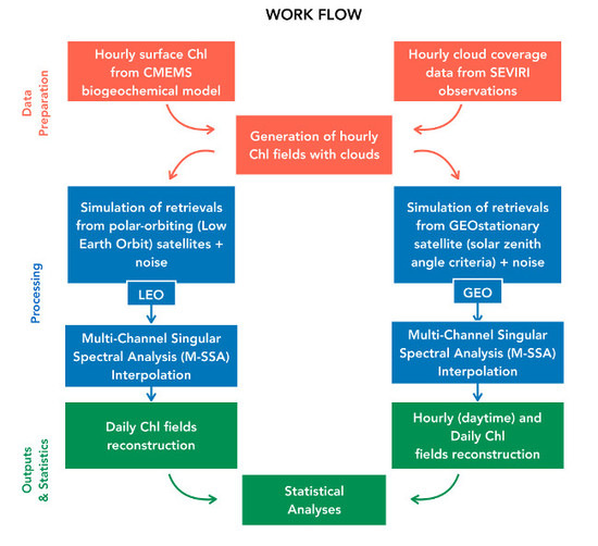
2. Materials and Methods

The approach developed here (the flowchart is illustrated in Figure 1) uses hourly Chl fields generated by numerical simulations and actual cloud distributions derived from the Spinning Enhanced Visible and Infrared Imager (SEVIRI) data. The area of study is located in the Baltic Sea (approximately 11° E to 24° E and 54° N to 60° N, Figure 2), for which modeled hourly Chl maps are distributed by the Copernicus Marine Environment Monitoring Service’s (CMEMS) Baltic Monitoring and Forecasting Centre (BAL MFC). SEVIRI data were used to create hourly cloud masks to be overlapped with the simulated Chl distributions to mimic observations from GEO and LEO sensors. Cloudy grid points were then interpolated using Multi-Channel Singular Spectral Analysis (M-SSA) [32,33] and interpolation errors were estimated comparing original modeled data masked using SEVIRI clouds with interpolated values in cases of hourly and daily fields. One could argue that the Baltic Sea is not optimally observed by a GEO sensor (because at these latitudes, the sun’s zenith angle would be very large and, for the most part, the view angle is greater compared to the tropical area). This issue is not critical because the Baltic Sea is used here as a case study. The main point is the use of realistic Chl distribution and hourly dynamics, provided by the model, and real cloud distributions, provided by SEVIRI.

A more detailed description of the different steps of the work is given below:

• Data preparation:

  ○

  Hourly surface Chl data of the biogeochemical model were extracted together with the hourly SEVIRI cloud masks.

  ○

  The Chl hourly fields were re-mapped on the SEVIRI observation grid.

  ○

  The hourly cloud masks were then overlaid on the hourly surface Chl fields.

• Processing:

  ○

  Simulation of a GEO sensor using the solar zenith angle criteria (see Section 2.3).

  ○

  Simulation of a LEO ocean color sensor, using the expected sampling time of the Sentinel-3A satellite over the study area. For simplicity, we have provided an over-sampling of a real LEO observations as we have included all the modelled Chl data that could potentially be beyond the swath of the sensor.

  ○

  A Gaussian noise was added on each single Chl data.

• Outputs and statistics:

  ○

  Reconstruction of hourly and daily Chl gap-free fields using the M-SSA technique [32,33].

  ○

  Estimation of bias and root mean square error between the reconstructed and original data fields.

2.1. Hourly Chl Simulated Data

We used one month (May 2016) of hourly simulated Chl data from the HIROMB BOOS biogeochemical Model (HBM) from the Copernicus Marine Environment Monitoring Service (CMEMS; BALTICSEA_ANALYSIS_FORECAST_BIO_003_007). For more details about the quality of the dataset, we refer the reader to the product user manual (http://marine.copernicus.eu/documents/PUM/CMEMS-BAL-PUM-003-007.pdf and the quality information document (http://marine.copernicus.eu/documents/QUID/CMEMS-BAL-QUID-003-007.pdf).

2.2. Hourly Clouds Data

Firstly, we applied real clouds to the modeled hourly surface Chl. Such clouds were obtained from the SEVIRI sensor on board METEOSAT. Data was downloaded from the IFREMER ftp server in GHRSST compliant L3C NetCDF4 format (ftp://eftp.ifremer.fr/cersat-rt/project/osi-saf). In this way, the result was similar to what we might get from satellite observations, in the visible band. Both datasets (i.e., Chl high frequency observations and clouds) were re-mapped over the SEVIRI observations grid.

2.3. Simulating GEO and LEO Retrievals

It was borne in mind that, due to atmospheric correction algorithm limits, only ocean color data with a solar zenith angle less than 70° is permitted [34,35] and that 70° is the maximum angle for which atmospheric correction algorithms based on plane–parallel radiative transfer calculations have been developed. Thus, the interpolation of data voids was conservatively limited to areas where the absolute value of the sun’s zenith angle was below 70°, excluding polar night conditions. Following this idea, we simulated observations from a GEO ocean color sensor selecting only daytime Chl observations (i.e., from approximately 07:00 to 16:00 local time; see Section 2). On the other hand, to simulate a single LEO sensor, only hourly fields of 12:00 and 13:00 local time were selected. Such time intervals include the typical polar satellite passes (i.e., 2 times per day in the case of a two-satellite configuration; see also https://sentinel.esa.int/web/sentinel/user-guides/sentinel-3-olci/coverage; see Section 2). Furthermore, a normally distributed noise (i.e., Gaussian noise) was added to each Chl field to obtain more realistic simulations of satellite Chl retrievals (see Section 2) [36], and references therein.

2.4. Multi-Channel Singular Spectral Analysis (M-SSA)

The M-SSA was used to fill gaps due to cloud coverage in the hourly data of the model-derived Chl [32,33]. The M-SSA technique is a non-parametric method relying on data only; i.e., it is not based on a priori parametrized family of probability distribution. The method uses both temporal and spatial correlation to fill in the missing data and represents a generalization of the [37] spatial empirical orthogonal functions-(EOFs) based reconstruction. It is particularly useful for datasets that exhibit gaps both in space and time, as is the case of satellite Chl retrievals. Kondrashov and Ghil (2006) demonstrated that an increased number of gaps yields the same effect as an increase of the noise in the measurements.

Two different inputs are required to apply M-SSA for field reconstruction: Window-length (W) and components (M). Both depend on the characteristics of the time series, and need to be accurately defined to avoid any bias in the reconstructed fields. The W represents the length of the sliding W-points window used in the M-SSA in order to identify the leading components of the time-series [32,33]. Diversely, M is the number of eigen-functions used for signal reconstruction.

Here, we applied the M-SSA to different cases: (i) Hourly Chl data for diel evolution reconstruction; and (ii) mean daytime Chl data for daily field reconstruction. In the first case, the M-SSA was applied on hourly GEO simulations using specific W (i.e., W = 48 h) and M components (i.e., M = 1 up to 6, that explains more than 95.0% of the variance) following the recommendations listed in [32,33]. These settings are compatible with the properties of the time series hereby analyzed, taking into account hourly variations. This method was not applied on the LEO simulations because of the limited spatial–temporal coverage (i.e., maximum two simulated images per day; see Section 3.2). In the second case, the M-SSA was used on Chl daily composites (i.e., for a total of 31 maps) for both GEO and LEO simulations using specific W and M components (i.e., W = 3 days and M = 1 up to 3, that explains more than 95.0% of the variance). For more details about the mathematical equations and theoretical principles at the base of the M-SSA method, see [32,33].

2.5. Statistical Indicators

The following statistical indicators have been used to quantify the differences between the LEO and GEO simulations, after the reconstruction that uses the M-SSA technique at hourly and daily scales:

(i)

The number of available simulations for the entire month for each pixel. This index directly allows us to quantify the potential observations as captured using a LEO versus GEO ocean color sensors;

(ii)

the bias and root mean square error between the original Chl and the gap-free reconstructed fields (in both the LEO and GEO cases) for diel Chl reconstructions and mean Chl daytime fields:

$$RMS=\sqrt{\frac{1}{N}{{\displaystyle \sum }}_{i=1}^N{\left(\frac{reconstructed-original}{original}\right)}^2}$$

$$BIAS=\frac{1}{N}{\displaystyle {{\displaystyle \sum }}_{i=1}^N}\left(reconstructed-original\right)$$

3. Results and Discussion

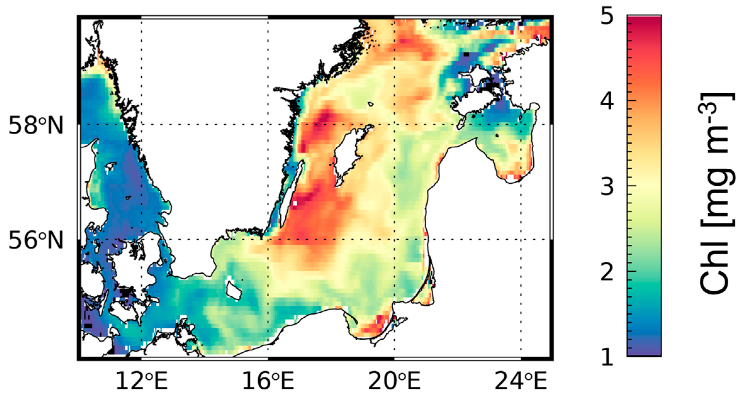
3.1. Chl Spatial–Temporal Distribution

The mean daytime reconstructed Chl field for May 2016 is shown in Figure 3. Chl concentrations ranged from 0.1 to 5 mg Chl m⁻³, consistent with the typical spring to summer values for this basin This period is between two distinct Chl maxima that typically occur at the end of April and in mid-July [38,39,40,41]. Higher values were located mostly at the center of the area of study (greater than 2 mg Chl m⁻³), while the lower Chl concentrations were distributed primarily at the southern and western parts of the basin (lower than 2 mg Chl m⁻³).

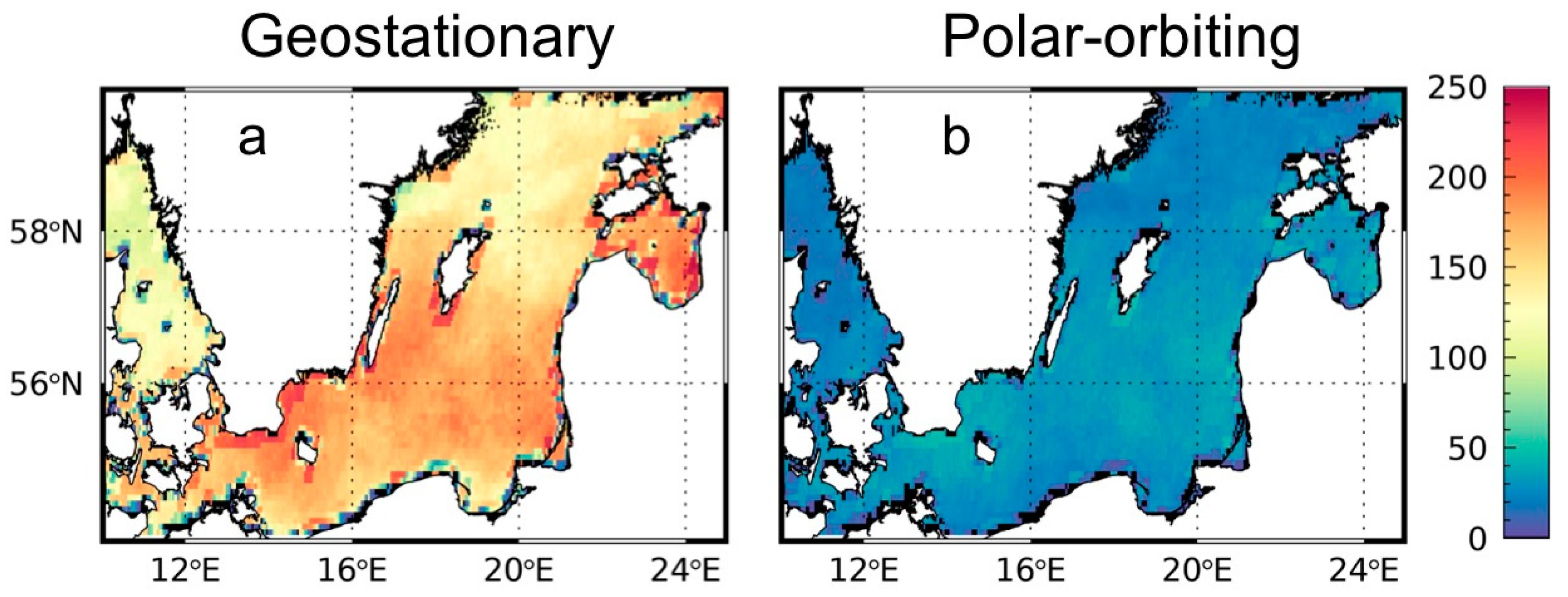
3.2. Spatial-Temporal Coverage

Figure 4 shows the ratio of valid pixels between GEO and LEO simulated daily maps for May 2016. As expected, the overall ratio was always greater than 1 and ranged between 1.1 (May 11th) and 4.1 on May 17th. It means that the GEO supported a better spatial coverage at daily scale. Daily maps derived from GEO had, on average, nearly twice the number of valid pixels with respect to daily maps in case of LEO (Figure 4).

Figure 5 shows the number of valid observations using high frequency data for May 2016 taking into account the real clouds on the area of study. At the eastern part of the basin, the number of hourly valid observations by GEO was around 100 per month per pixel, while in the central part of the area of study, the number of hourly GEO valid observations for each pixel was larger than 150 per month. Consequently, in the case of a LEO sensor, the number of observations for each pixel was always lower than 62 per month due to the limited number of retrievals (i.e., maximum two per day) and the cloud impact.

3.3. Hourly Reconstruction

Figure 6 shows the behavior of Chl daytime fields as a function of solar zenith angles. Individual Chl values were binned by intervals of solar zenith angles for three different cases: (i) Cloudy Chl fields reconstructed via M-SSA; (ii) the original gap-free modelled Chl fields and (iii) the modelled Chl with cloudy pixels, not reconstructed. In the first and second case, the number of data used to compute the average, in each interval, was the same and equal to the maximum number of possible observations in the absence of clouds. In the third case, the data used for the average, in each single interval, varied according to the cloud coverage. The correlation between the reconstructed and the original model fields was excellent and the differences were limited, as also shown in Figure 7. There was a clear Chl increase from 1.9 mg m⁻³ to 2.65 mg m⁻³ (maximum value) when the solar zenith angle increased from 30° to 45°. Chl remained in a steady state, and then decreased again for angles greater than 65°. Observing from space, these results can be achieved solely by using a GEO sensor, while, conversely, with the LEO, only a few points can be retrieved due to limited temporal coverage, and thus such evolution cannot be detected. Figure 6 also shows how less accurate Chl estimates can be obtained using model-gapped fields, i.e., with less observations, average computations are limited due to clouds.

Figure 7 represents the RMS and bias between reconstructed Chl and original modeled hourly fields in the case of a GEO sensor. The RMS map shows values greater than 1 mg m⁻³ at the northern border (latitude greater than 58°) of the area of study. The average value is 0.21 mg m⁻³ (Figure 7a). In the central and southern parts of the basin, the RMS was generally lower than ~0.2 mg Chl m⁻³.

The bias map shows an efficient estimation of hourly Chl fields after the reconstruction, which in a few limited areas reached values of ~0.2 to 0.4 mg Chl m⁻³. In addition, the northern part of the study area shows negative biases larger than −0.2 mg Chl m⁻³, in correspondence with the highest RMS values. However, most of the values ranged from −0.1 to +0.1 mg Chl m⁻³. Indeed, the bias had a positive value close to 0. Concerning the RMS and bias errors, the M-SSA interpolation method exhibited the best performance at lower and middle latitudes and open ocean water.

3.4. Mean Daytime Reconstruction

Figure 8a,b represent the RMS error between the reconstructed and the original daily Chl fields estimated in cases of LEO and GEO sensors, respectively, for the series of 31 Chl maps in May 2016. It means that in the first case, (Figure 8a) each of the 31 daily means was derived from a maximum of two observations per day; in the second case (Figure 8b), each daily mean was derived from several hourly observations. For consistency, the M-SSA was applied on the daily mean, and not on each hourly average as in the Section 3.3. The RMS had average values of 0.18 mg Chl m⁻³ and 0.26 mg Chl m⁻³, respectively for the GEO and LEO sensors. These interpolation errors were half with respect to the RMS evaluated for the current CMEMS satellite Chl product in the Baltic Sea (0.4 to 0.5 mg Chl m⁻³; see Table 7 in http://cmems-resources.cls.fr/documents/QUID/CMEMS-OC-QUID-009-048-049.pdf). The order of magnitude was, however, similar. In the northern part, the RMS was close to 0.4 mg Chl m⁻³ for the GEO sensor, but still strongly reduced with respect to the LEO sensor (0.7 mg Chl m⁻³). Thus, the main result is that there was a potential decrease of around 50% of the RMS for a GEO sensor in the area of highest errors for a LEO sensor. Using more observations and for the daily Chl map, the reconstruction enabled us to reproduce the original field with fewer errors: The daily Chl field was close to reproducing the model-derived field. Increasing the number of observations can be of great value in the case of data assimilation models, especially with regards to the quality of biogeochemical daily products. Figure 8c shows how, at higher latitudes, the relative differences tended to be larger than 60%, whereas in the southern part of the basin, the relative differences were generally between 1% and 10%, reflecting the distribution of clouds.

4. Conclusions and Final Remarks

The main goal of the study was to quantify the benefits of having high-temporal resolution observations from space in order to reduce errors in the reconstructed surface hourly and daily Chl fields in the Baltic Sea. To this aim, we have developed a new method to simulate satellite-derived observations by combining outputs from a biogeochemical numerical model with real cloud distributions. As a first step, we have imitated geostationary satellite measurements using hourly data from one biogeochemical model available in the Baltic Sea (i.e., HIROMB BOOS Model from Copernicus Marine Environment Monitoring Service). The hourly cloud masks obtained from SEVIRI were overlapped to all Chl simulations. Following this, the Multi-Channel Singular Spectral Analysis (M-SSA) was applied to fill in the data gaps caused by the cloud distributions, finally obtaining gap-free Chl hourly maps. Specifically, two cases are discussed: (i) The simulation of observations from one LEO ocean color sensor and (ii) the simulation of observations from one GEO satellite sensor with hourly acquisitions for acceptable solar zenith angles. Results show that a GEO sensor enabled us to detect the diel Chl evolution (Figure 6) with reduced and acceptable RMS and bias interpolation errors (Figure 7). The LEO sensor cannot do this due to the limited spatial and temporal coverages and the limited number of possible observations (Figure 4 and Figure 5). In addition, considering the daily Chl field, the RMS and bias decreased significantly using GEO-based simulations with respect to a single LEO counterpart. In detail, in some areas (Figure 8a,b), the spatial RMS error was reduced by more than 50% using a GEO instead of a LEO sensor. Such analysis highlights the importance of high-frequency observations to capture and weigh the information that, otherwise, may be lost using only a few ocean color satellite observations per day. Future research will focus on: (i) The use of a longer time-series (i.e., from months to years) in order to take into account the Chl seasonal and annual cycles in the M-SSA interpolation method; (ii) the application of the method on the tropics and mid-latitudes, in order to test the results under higher solar altitudes and (iii) the application of the present method to real ocean color geostationary data (i.e., GOCI-I) in comparison with a real LEO ocean color satellite dataset over the same study area.

References

1. Martinez, E.; Antoine, D.; D’Ortenzio, F.; Gentili, B. Climate-driven basin-scale decadal oscillations of oceanic phytoplankton. Science 2009, 326, 1253–1256. [Google Scholar] [CrossRef] [PubMed]
2. Behrenfeld, M.J.; O’Malley, R.T.; Boss, E.S.; Westberry, T.K.; Graff, J.R.; Halsey, K.H.; Milligan, A.J.; Siegel, D.A.; Brown, M.B. Revaluating ocean warming impacts on global phytoplankton. Nat. Clim. Chang. 2016, 6, 323. [Google Scholar] [CrossRef]
3. Organelli, E.; Claustre, H.; Bricaud, A.; Schmechtig, C.; Poteau, A.; Xing, X.; Prieur, L.; D’Ortenzio, F.; Dall’Olmo, G.; Vellucci, V. A novel near-real-time quality-control procedure for radiometric profiles measured by Bio-Argo floats: Protocols and performances. J. Atmos. Ocean. Technol. 2016, 33, 937–951. [Google Scholar] [CrossRef]
4. Barbieux, M.; Uitz, J.; Bricaud, A.; Organelli, E.; Poteau, A.; Schmechtig, C.; Gentili, B.; Obolensky, G.; Leymarie, E.; Penkerc’h, C.; D’Ortenzio, F. Assessing the Variability in the Relationship between the Particulate Backscattering Coefficient and the Chlorophyll a Concentration from a Global Biogeochemical-Argo Database. J. Geophys. Res. Oceans 2018, 123, 1229–1250. [Google Scholar] [CrossRef]
5. Antoine, D.; D’Ortenzio, F.; Hooker, S.B.; Becu, G.; Gentili, B.; Tailliez, D.; Scott, A.J. Assessment of uncertainty in the ocean reflectance determined by three satellite ocean color sensors (MERIS, SeaWiFS and MODIS-A) at an offshore site in the Mediterranean Sea (BOUSSOLE project). J. Geophys. Res. 2008, 113, C07013. [Google Scholar] [CrossRef]
6. Antoine, D.; Guevel, P.; Deste, J.F.; Becu, G.; Louis, F.; Scott, A.J.; Bardey, P. The ‘‘BOUSSOLE’’ buoy—A new transparent-to-swell taut mooring dedicated to marine optics: Design, tests, and performance at sea. J. Atmos. Oceanic Technol. 2008, 25, 968–989. [Google Scholar] [CrossRef]
7. Antoine, D.; Siegel, D.A.; Kostadinov, T.; Maritorena, S.; Nelson, N.B.; Gentili, B.; Vellucci, V.; Guillocheau, N. Variability in optical particle backscattering in contrasting bio-optical oceanic regimes. Limnol. Oceanogr. 2011, 56, 955–973. [Google Scholar] [CrossRef] [Green Version]
8. Volpe, G.; Nardelli, B.B.; Colella, S.; Santoleri, R. An Operational Interpolated Ocean Colour Product in the Mediterranean Sea. In GODAE Oceanview International School in “New Frontiers in Operational Oceanography”; Chassignet, E.P., Pascual, A., Tintore, J., Verron, J., Eds.; GODAE OceanView, 2018; pp. 227–244. [Google Scholar] [CrossRef]
9. Neveux, J.; Dupouy, C.; Blanchot, J.; Le Bouteiller, A.; Landry, M.R.; Brown, S.L. Diel dynamics of chlorophylls in high-nutrient, low-chlorophyll waters of the equatorial Pacific (180°): Interactions of growth, grazing, physiological responses, and mixing. J. Geophys. Res. Oceans 2003, 108. [Google Scholar] [CrossRef] [Green Version]
10. Oubelkheir, K.; Sciandra, A. Diel variations in particle stocks in the oligotrophic waters of the Ionian Sea (Mediterranean). J. Mar. Syst. 2008, 74, 364–371. [Google Scholar] [CrossRef]
11. Dall’Olmo, G.; Boss, E.; Behrenfeld, M.J.; Westberry, T.K.; Courties, C.; Prieur, L.; Pujo-Pay, M.; Hardman-Mountford, N.; Moutin, T. Inferring phytoplankton carbon and eco-physiological rates from diel cycles of spectral particulate beam-attenuation coefficient. Biogeosciences 2011, 8, 3423–3439. [Google Scholar] [CrossRef]
12. Loisel, H.; Vantrepotte, V.; Norkvist, K.; Meriaux, X.; Kheireddine, M.; Ras, J.; Pujo-Pay, M.; Combet, Y.; Leblanc, K.; Dall’Olmo, G.; et al. Characterization of the bio-optical anomaly and diurnal variability of particulate matter, as seen from scattering and backscattering coefficients, in ultra-oligotrophic eddies of the Mediterranean Sea. Biogeosciences 2011, 8, 3295–3317. [Google Scholar] [CrossRef] [Green Version]
13. Gernez, P.; Antoine, D.; Huot, Y. Diel cycles of the particulate beam attenuation coefficient under varying trophic conditions in the northwestern Mediterranean Sea: Observations and modeling. Limnol. Oceanogr. 2011, 56, 17–36. [Google Scholar] [CrossRef]
14. Barnes, M.; Antoine, D. Proxies of community production derived from the diel variability of particulate attenuation and backscattering coefficients in the northwest Mediterranean Sea. Limnol. Oceanogr. 2014, 59, 2133–2149. [Google Scholar] [CrossRef]
15. Kheireddine, M.; Antoine, D. Diel variability of the beam attenuation and backscattering coefficients in the northwestern Mediterranean Sea (BOUSSOLE site). J. Geophys. Res. Oceans 2014, 119, 5465–5482. [Google Scholar] [CrossRef] [Green Version]
16. Poulin, C.; Antoine, D.; Huot, Y. Diurnal variations of the optical properties of phytoplankton in a laboratory experiment and their implication for using inherent optical properties to measure biomass. Opt. Express 2018, 26, 711–729. [Google Scholar] [CrossRef]
17. Constantin, S.; Doxaran, D.; Derkacheva, A.; Novoa, S.; Lavigne, H. Multi-temporal dynamics of suspended particulate matter in a macro-tidal river Plume (the Gironde) as observed by satellite data. Estuar. Coast. Shelf Sci. 2018, 202, 172–184. [Google Scholar] [CrossRef]
18. Stramska, M.; Dickey, T.D. Variability of bio-optical properties of the upper ocean associated with diel cycles in phytoplankton population. J. Geophys. Res. 1992, 97, 17873–17887. [Google Scholar] [CrossRef]
19. Arnone, R.A.; Vandermeulen, R.A.; Soto, I.M.; Ladner, S.D.; Ondrusek, M.E.; Yang, H. Diurnal changes in ocean color sensed in satellite imagery. J. Appl. Remote Sens. 2017, 11, 032406. [Google Scholar] [CrossRef] [Green Version]
20. IOCCG. Ocean-Colour Observations from a Geostationary Orbit. In Reports of the International Ocean-Colour Coordinating Group; Antoine, D., Ed.; No. 12; IOCCG: Dartmouth, NS, Canada, 2012. [Google Scholar]
21. Neukermans, G.; Ruddick, K.G.; Greenwood, N. Diurnal variability of turbidity and light attenuation in the southern North Sea from the SEVIRI geostationary sensor. Remote Sens. Environ. 2012, 124, 564–580. [Google Scholar] [CrossRef]
22. Ruddick, K.; Neukermans, G.; Vanhellemont, Q.; Jolivet, D. Challenges and opportunities for geostationary ocean colour remote sensing of regional seas: A review of recent results. Remote Sens. Environ. 2014, 146, 63–76. [Google Scholar] [CrossRef]
23. Marullo, S.; Santoleri, R.; Banzon, V.; Evans, R.H.; Guarracino, M. A diurnal-cycle resolving sea surface temperature product for the tropical Atlantic. J. Geophys. Res. Oceans 2010, 115. [Google Scholar] [CrossRef] [Green Version]
24. Marullo, S.; Santoleri, R.; Ciani, D.; Le Borgne, P.; Péré, S.; Pinardi, N.; Tonani, M.; Nardone, G. Combining model and geostationary satellite data to reconstruct hourly SST field over the Mediterranean Sea. Remote Sens. Environ. 2014, 146, 11–23. [Google Scholar] [CrossRef]
25. Marullo, S.; Minnett, P.J.; Santoleri, R.; Tonani, M. The diurnal cycle of sea-surface temperature and estimation of the heat budget of the Mediterranean Sea. J. Geophys. Res. Oceans 2016, 121, 8351–8367. [Google Scholar] [CrossRef]
26. Lamquin, N.; Mazeran, C.; Doxaran, D.; Ryu, J.H.; Park, Y.J. Assessment of GOCI radiometric products using MERIS, MODIS and field measurements. Ocean Sci. J. 2012, 47, 287–311. [Google Scholar] [CrossRef]
27. Wang, M.; Ahn, J.H.; Jiang, L.; Shi, W.; Son, S.; Park, Y.J.; Ryu, J.H. Ocean color products from the Korean geostationary ocean color imager (GOCI). Opt. Express 2013, 21, 3835–3849. [Google Scholar] [CrossRef] [PubMed]
28. Lou, X.; Hu, C. Diurnal changes of a harmful algal bloom in the East China Sea: Observations from GOCI. Remote Sens. Environ. 2014, 140, 562–572. [Google Scholar] [CrossRef]
29. Choi, J.K.; Park, Y.J.; Lee, B.R.; Eom, J.; Moon, J.E.; Ryu, J.H. Application of the Geostationary Ocean Color Imager (GOCI) to mapping the temporal dynamics of coastal water turbidity. Remote Sens. Environ. 2014, 146, 24–35. [Google Scholar] [CrossRef]
30. Amin, R.; Lewis, M.D.; Lawson, A.; Gould Jr, R.W.; Martinolich, P.; Li, R.R.; Ladner, S.; Gallegos, S. Comparative Analysis of GOCI Ocean Color Products. Sensors 2015, 15, 25703–25715. [Google Scholar] [CrossRef] [Green Version]
31. Jiang, L.; Wang, M. Diurnal Currents in the Bohai Sea Derived from the Korean Geostationary Ocean Color Imager. IEEE Trans. Geosci. Remote Sens. 2017, 55, 1437–1450. [Google Scholar] [CrossRef]
32. Ghil, M.; Allen, M.R.; Dettinger, M.D.; Ide, K.; Kondrashov, D.; Mann, M.E.; Robertson, A.W.; Saunders, A.; Tian, Y.; Varadi, F.; et al. Advanced spectral methods for climatic time series. Rev. Geophys. 2002, 40, 3-1–3-41. [Google Scholar] [CrossRef] [Green Version]
33. Kondrashov, D.; Ghil, M. Spatio-temporal filling of missing points in geophysical data sets. Nonlinear Processes Geophys. 2006, 13, 151–159. [Google Scholar] [CrossRef] [Green Version]
34. Wang, M.; Gordon, H.R. Calibration of ocean color scanners: How much error is acceptable in the near infrared? Remote Sens. Environ. 2002, 82, 497–504. [Google Scholar] [CrossRef]
35. Gregg, W.W.; Casey, N.W. Sampling biases in MODIS and SeaWiFS ocean chlorophyll data. Remote Sens. Environ. 2007, 111, 25–35. [Google Scholar] [CrossRef] [Green Version]
36. Barbu, T. Variational image denoising approach with diffusion porous media flow. In Abstract and Applied Analysis; Hindawi: Cairo, Egypt, 2013. [Google Scholar]
37. Beckers, J.M.; Rixen, M. EOF calculations and data filling from incomplete oceanographic datasets. J. Atmos. Ocean. Technol. 2003, 20, 1839–1856. [Google Scholar] [CrossRef]
38. Wan, Z.; Jonasson, L.; Bi, H. N/P ratio of nutrient uptake in the Baltic Sea. Ocean Sci. 2011, 7, 693–704. [Google Scholar] [CrossRef] [Green Version]
39. Pitarch, J.; Volpe, G.; Colella, S.; Krasemann, H.; Santoleri, R. Remote sensing of chlorophyll in the Baltic Sea at basin scale from 1997 to 2012 using merged multi-sensor data. Ocean Sci. 2016, 12, 379–389. [Google Scholar] [CrossRef]
40. Schneider, B.; Kaitala, S.; Maunula, P. Identification and quantification of plankton bloom events in the Baltic Sea by continuous pCO2 and chlorophyll-a measurements on a cargo ship. J. Mar. Syst. 2006, 59, 238–248. [Google Scholar] [CrossRef]
41. Reissmann, J.H.; Burchard, H.; Feistel, R.; Hagen, E.; Lass, H.U.; Mohrholz, V.; Nausch, G.; Umlauf, L.; Wieczorek, G. Vertical mixing in the Baltic Sea and consequences for eutrophication—A review. Prog. Oceanogr. 2009, 82, 47–80. [Google Scholar] [CrossRef]
Figure 1. Flowchart diagram of the method developed in this paper. Orange represents dataset preparation, blue represents the processing of data, and green represents the outputs and statistical analyses.
Remotesensing 10 01944 g001
Figure 2. Example chlorophyll-a concentration (Chl) maps: (a) As obtained from the HBM HBO model for the 1 May 2016 at 12:00 local time; and (b) after the application of cloud masks (in white) by SEVIRI imager at the same hour.
Remotesensing 10 01944 g002
Figure 3. The mean daytime Chl field for May 2016 from the biogeochemical model after reconstruction of gaps with the Multi-Channel Singular Spectral Analysis (M-SSA) method using observations from a geostationary (GEO) simulation.
Remotesensing 10 01944 g003
Figure 4. Ratio between the number of valid pixels, in each daily Chl map, derived from GEO and low-Earth orbit (LEO) sensors from May 2016. A valid pixel is defined as a pixel where, at least, a daily Chl mean value has been estimated.
Remotesensing 10 01944 g004
Figure 5. Number of valid observations in case of GEO (a) and LEO (b) in May 2016. Observations with solar zenith angles greater than 70° were excluded.
Remotesensing 10 01944 g005
Figure 6. Chl variability as a function of the solar zenith angle (in degrees) using mean Chl GEO retrievals after reconstruction with M-SSA (in yellow) in comparison to the original modeled Chl fields (in cyan) and the model Chl with clouds over-imposed (in grey).
Remotesensing 10 01944 g006
Figure 7. RMS and bias reconstruction errors using the entire time-series of daylight hourly observations with respect to the original hourly fields, in a GEO context.
Remotesensing 10 01944 g007
Figure 8. RMS reconstruction error for daily Chl field in case of LEO (a) and GEO (b) sensors. Panel (c) represents the relative differences between RMS of LEO and GEO.
Remotesensing 10 01944 g008