Uncertainties in the Geostationary Ocean Color Imager (GOCI) Remote Sensing Reflectance for Assessing Diurnal Variability of Biogeochemical Processes


Abstract
1. Introduction
2. Data and Sensor Characteristics
2.1. GOCI Data
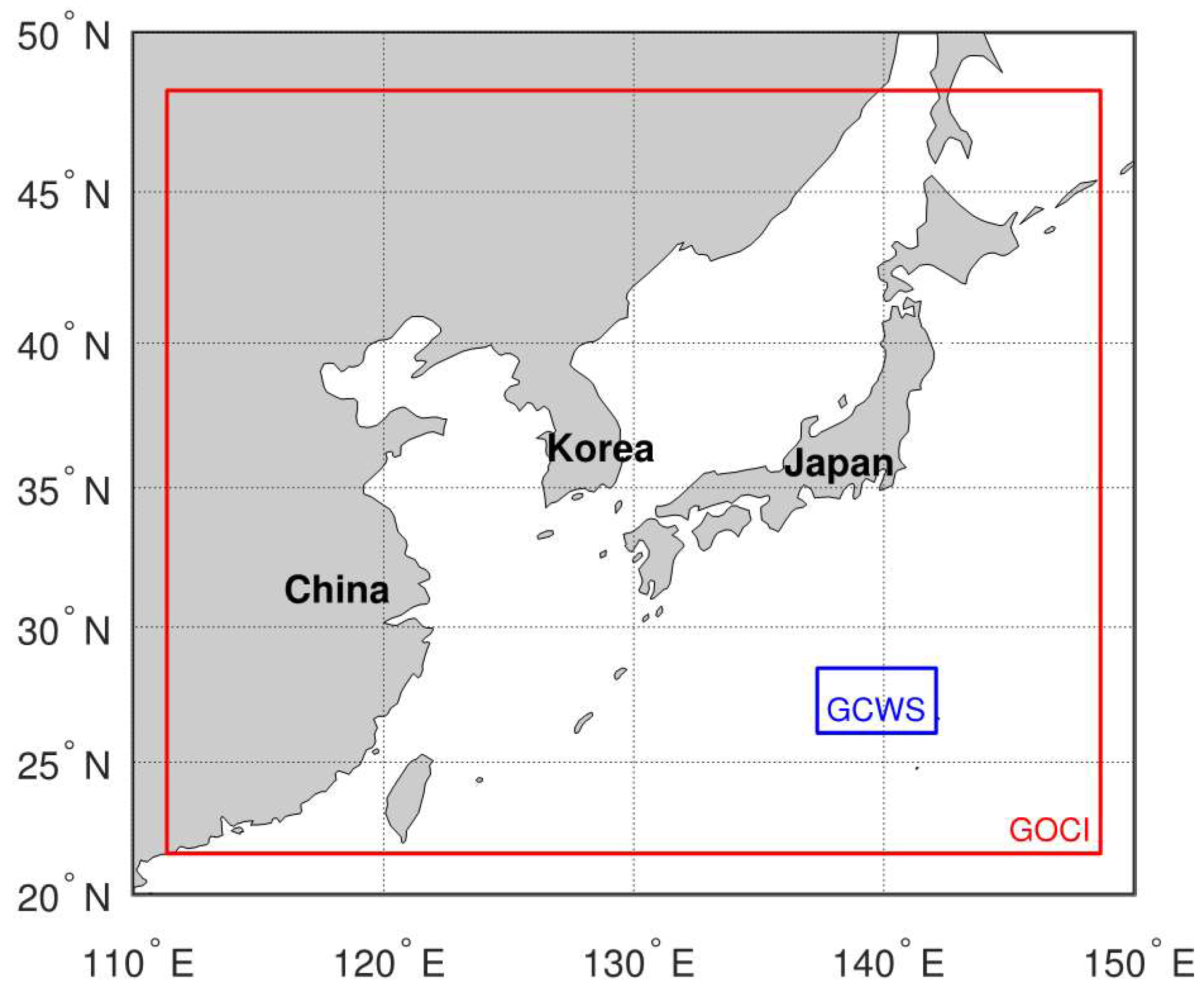
2.2. Area of Study
3. Processing Approach
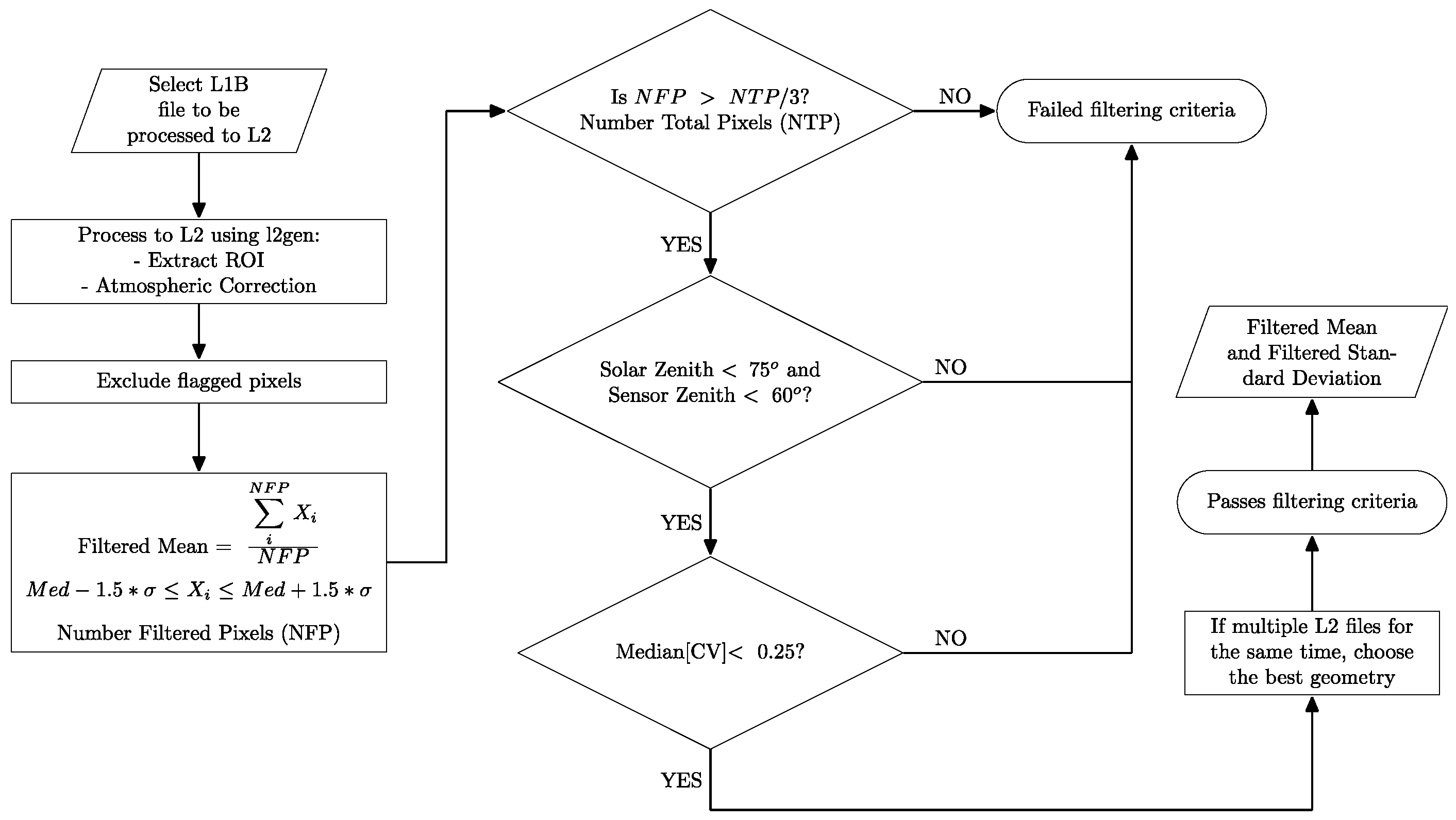
3.1. Conversion to Level 2
3.2. Data Screening
3.3. Bio-Optical Algorithms
3.3.1. Chlorophyll-a Concentration (Chl-a)
3.3.2. Particulate Organic Carbon (POC)
3.3.3. Chromophoric Dissolved Organic Matter Absorption Coefficient at 412 nm (ag(412))
4. Results and Discussion
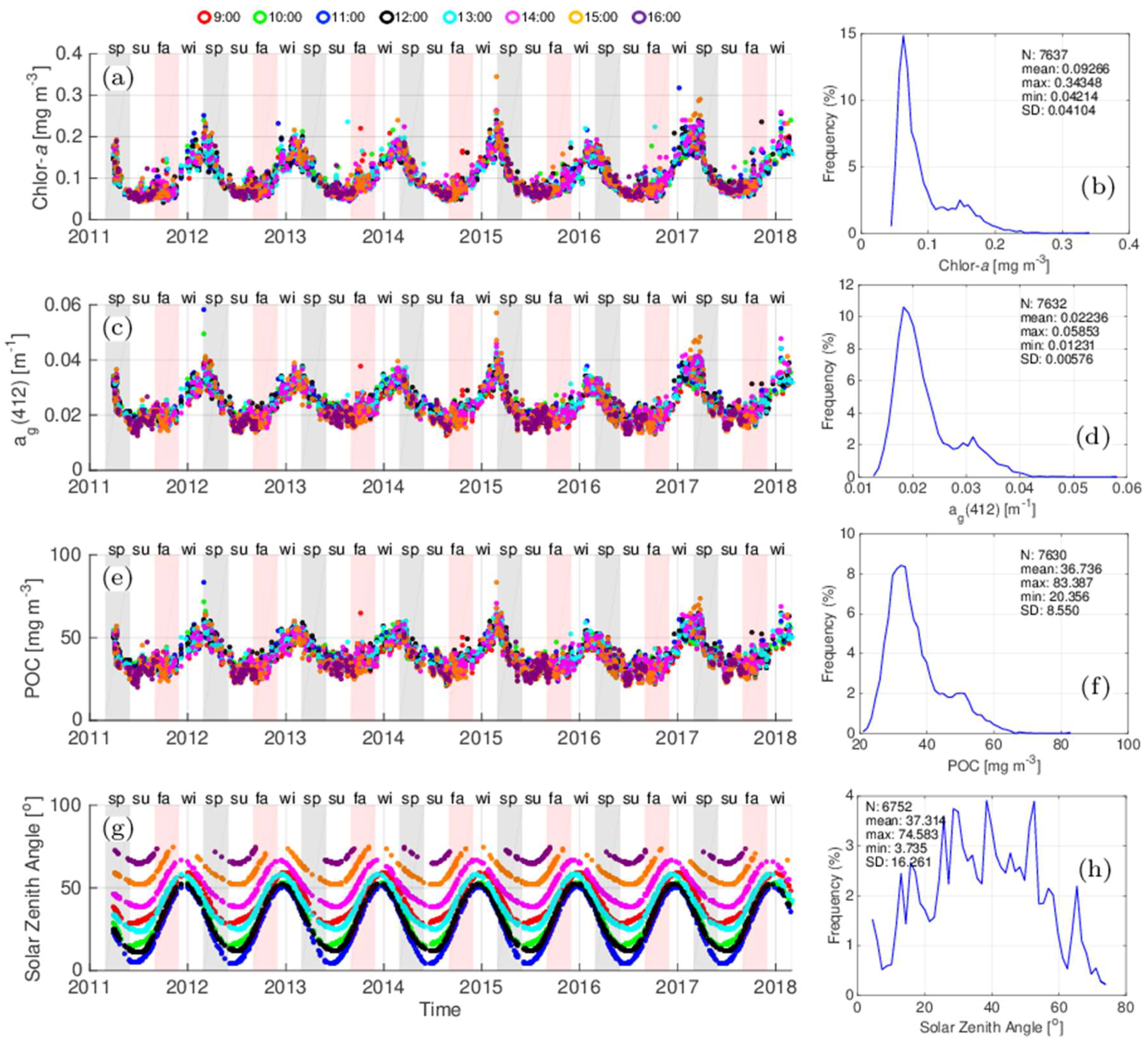
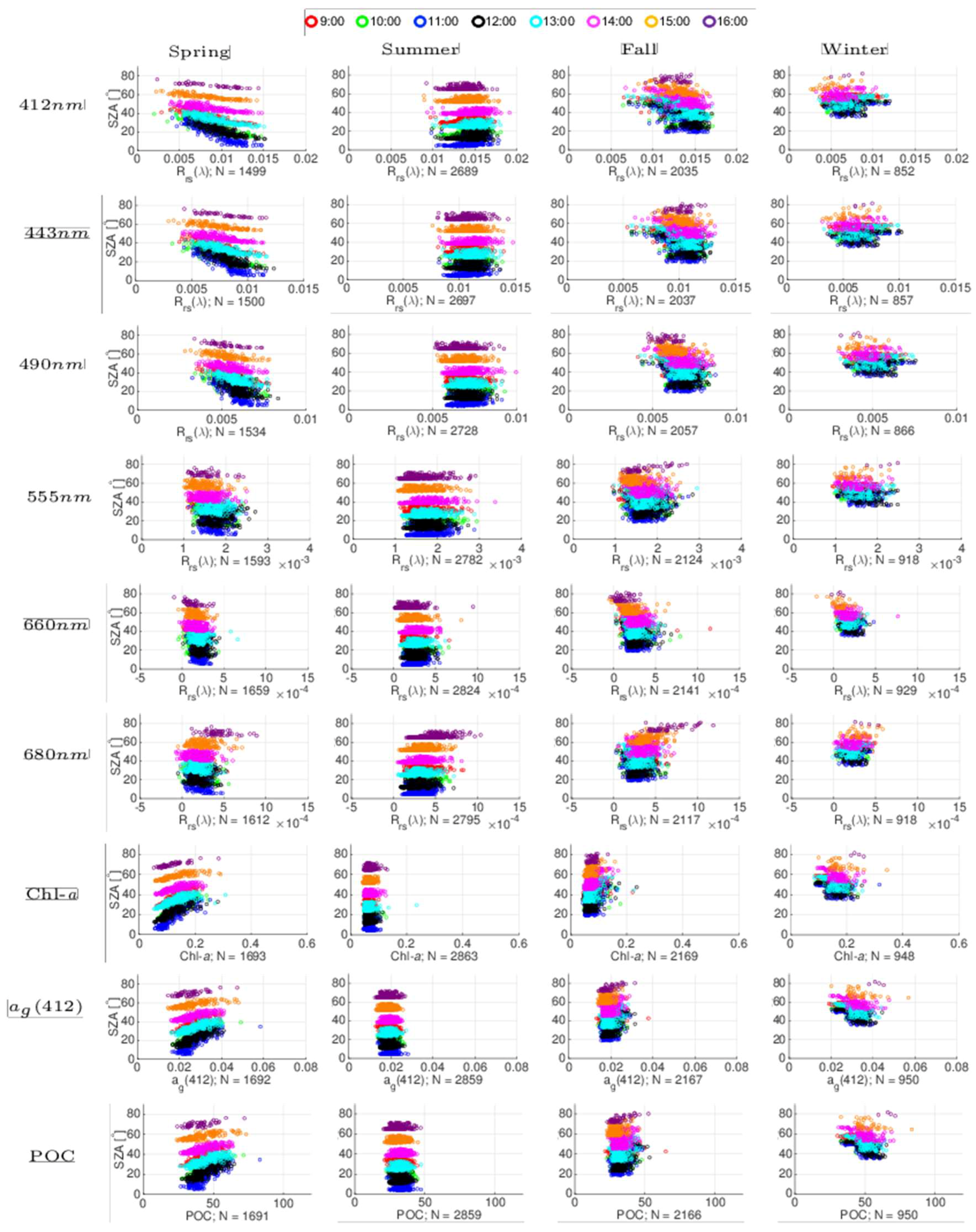
4.1. Seasonality
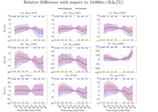
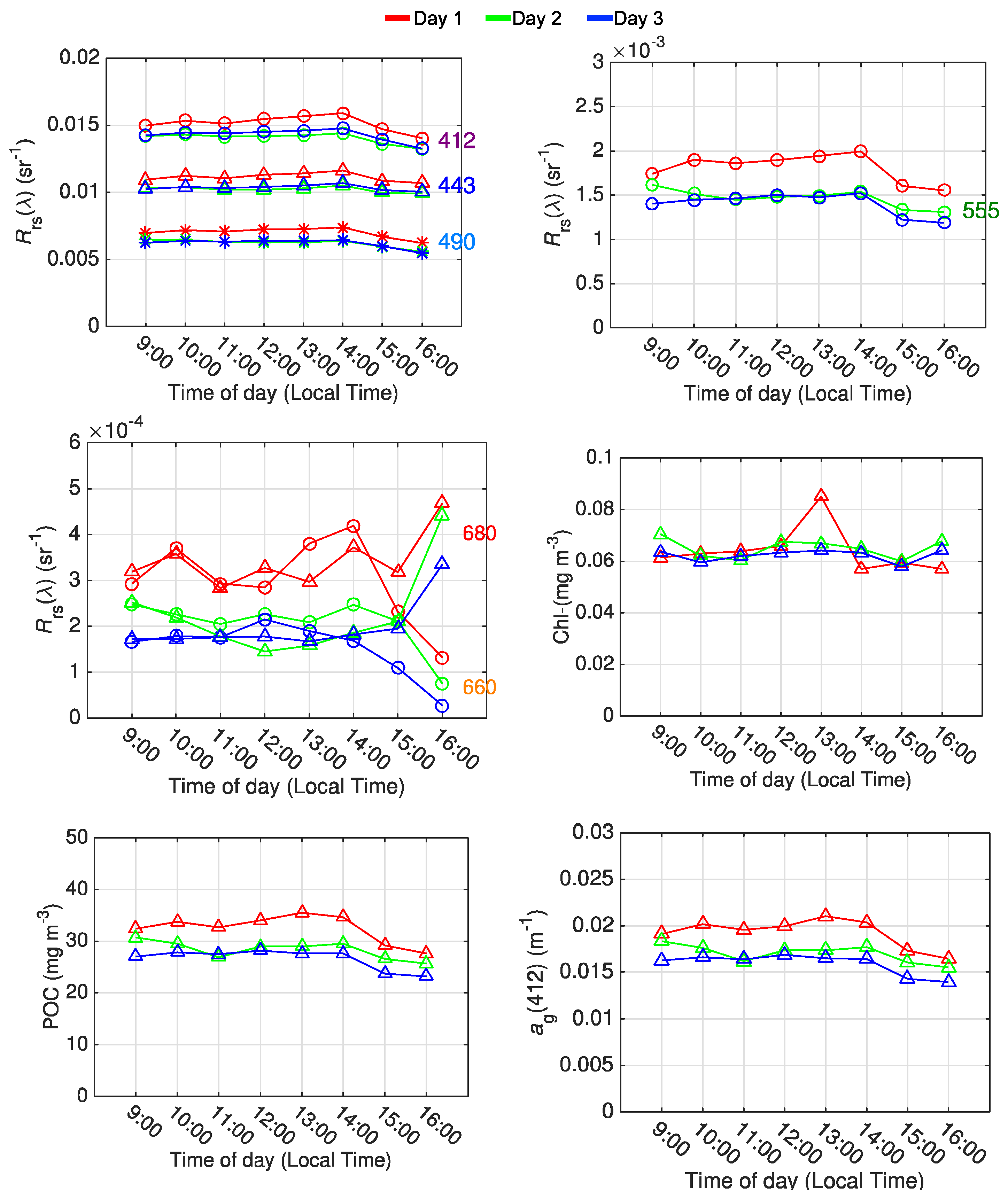
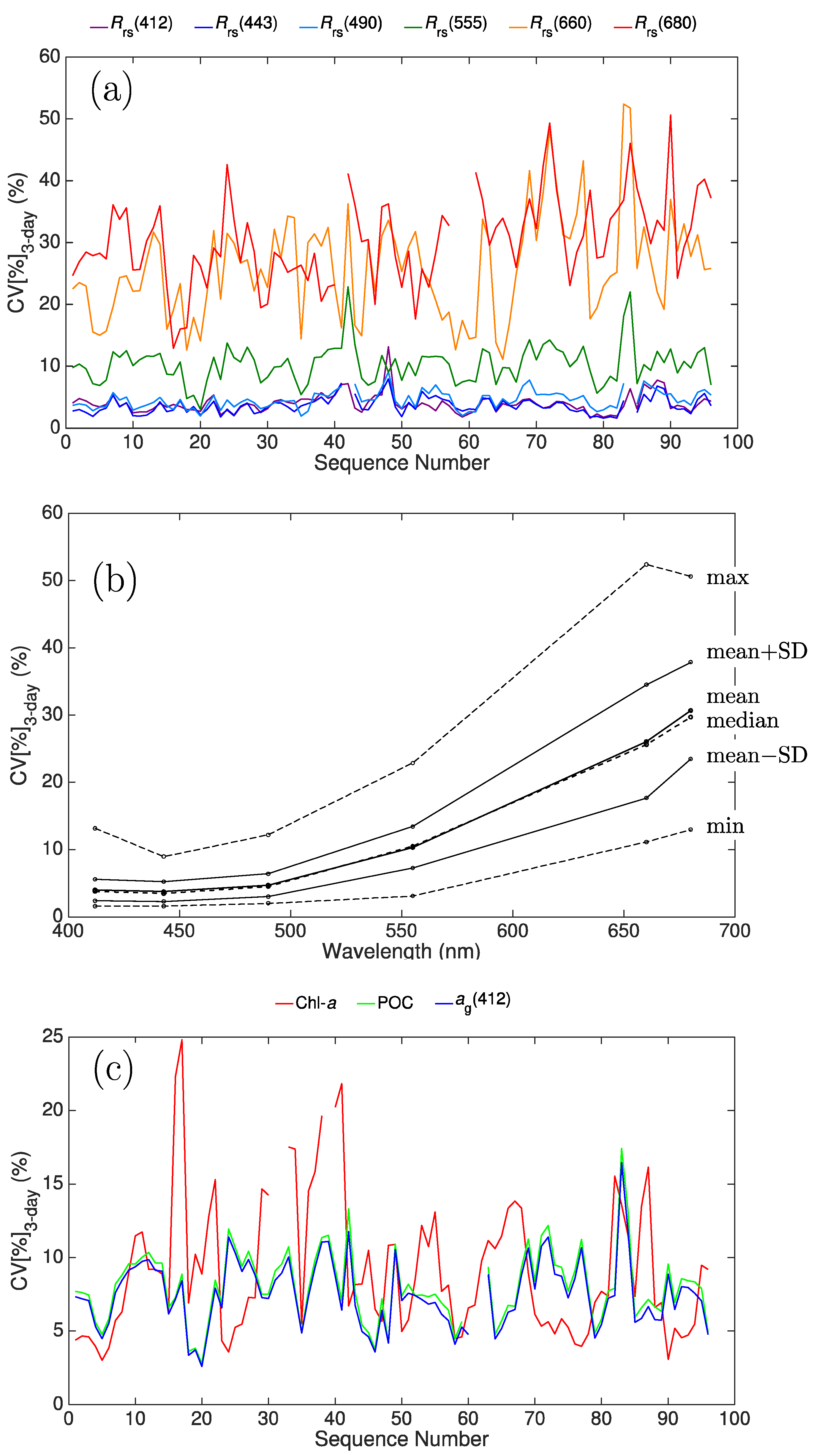
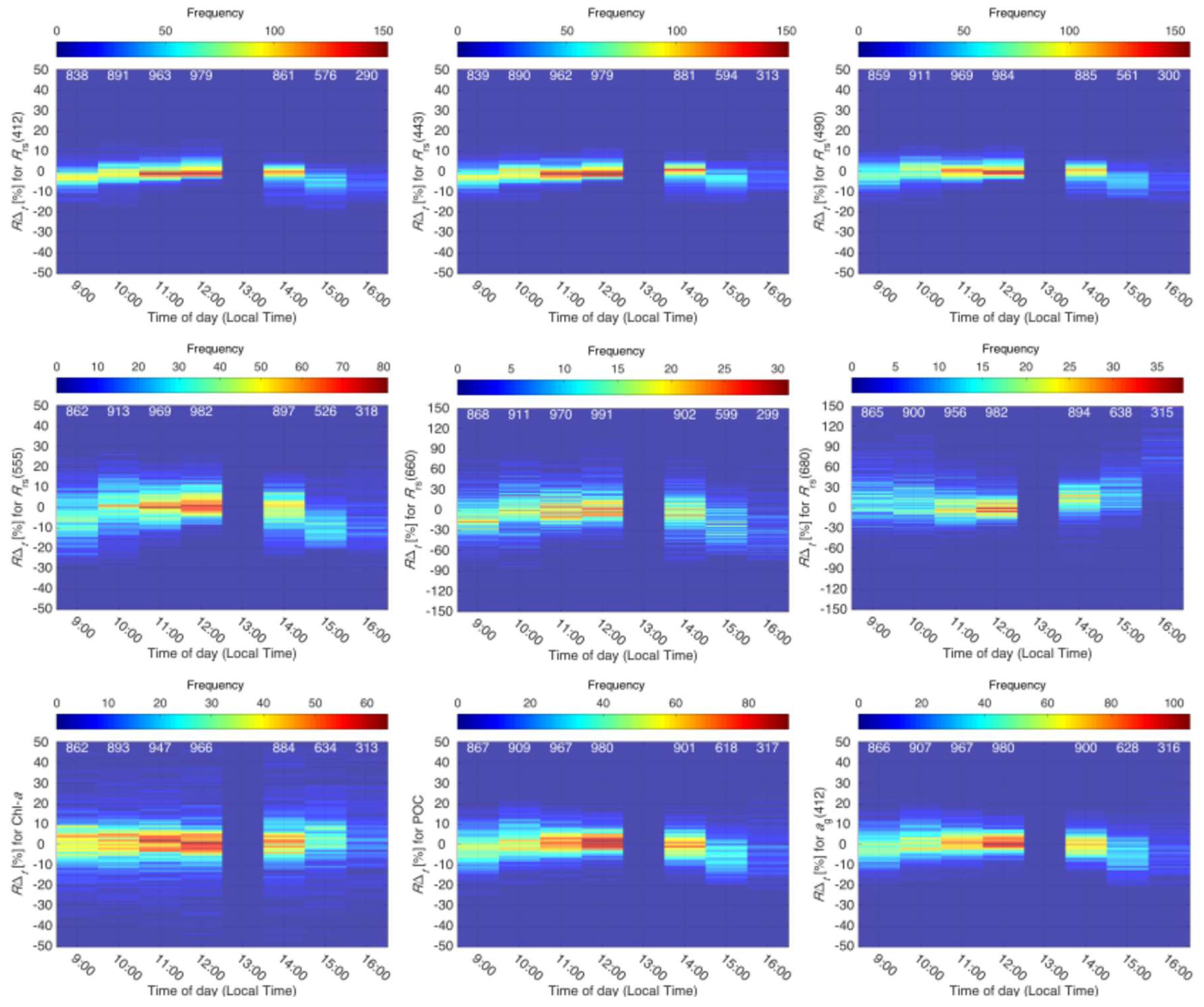
4.2. Diurnal and Day-to-Day Variability
5. Summary and Conclusions
Author Contributions
Funding
Acknowledgments
Conflicts of Interest
References
- McClain, C.R. A Decade of Satellite Ocean Color Observations. Annu. Rev. Mar. Sci. 2009, 1, 19–42. [Google Scholar] [CrossRef] [PubMed]
- Lee, Z.; Shang, S.; Hu, C.; Lewis, M.; Arnone, R.; Li, Y.; Lubac, B. Time series of bio-optical properties in a subtropical gyre: Implications for the evaluation of interannual trends of biogeochemical properties. J. Geophys. Res. Oceans 2010, 115. [Google Scholar] [CrossRef]
- Behrenfeld, M.J.; O’Malley, R.T.; Boss, E.S.; Westberry, T.K.; Graff, J.R.; Halsey, K.H.; Milligan, A.J.; Siegel, D.A.; Brown, M.B. Revaluating ocean warming impacts on global phytoplankton. Nat. Clim. Chang. 2016, 6, 323–330. [Google Scholar] [CrossRef]
- Mélin, F.; Sclep, G.; Jackson, T.; Sathyendranath, S. Uncertainty estimates of remote sensing reflectance derived from comparison of ocean color satellite data sets. Remote Sens. Environ. 2016, 177, 107–124. [Google Scholar] [CrossRef]
- Hooker, S.B.; Esaias, W.E.; Feldman, G.C.; Gregg, W.W.; McClain, C.R. An Overview of SeaWiFS and Ocean Color; SeaWiFS Technical Report Series, Volume 1 NASA Tech. Memo. 104566; NASA Goddard Space Flight Center: Greenbelt, MD, USA, 1992. [Google Scholar]
- Esaias, W.; Abbott, M.; Barton, I.; Brown, O.B.; Campbell, J.; Carder, K.; Clark, D.; Evans, R.; Hoge, F.E.; Gordon, H.; et al. An overview of MODIS capabilities for ocean science observations. IEEE Trans. Geosci. Remote Sens. 1998, 36, 1250–1265. [Google Scholar] [CrossRef]
- Goldberg, M.D.; Kilcoyne, H.; Cikanek, H.; Mehta, A. Joint Polar Satellite System: The United States next generation civilian polar-orbiting environmental satellite system. J. Geophys. Res. Atmos. 2013, 118, 13463–13475. [Google Scholar] [CrossRef]
- Loisel, H.; Vantrepotte, V.; Norkvist, K.; Mériaux, X.; Kheireddine, M.; Ras, J.; Pujo-Pay, M.; Combet, Y.; Leblanc, K.; Dall’Olmo, G.; et al. Characterization of the bio-optical anomaly and diurnal variability of particulate matter, as seen from scattering and backscattering coefficients, in ultra-oligotrophic eddies of the Mediterranean Sea. Biogeosciences 2011, 8, 3295–3317. [Google Scholar] [CrossRef]
- Ruddick, K.; Neukermans, G.; Vanhellemont, Q.; Jolivet, D. Challenges and opportunities for geostationary ocean colour remote sensing of regional seas: A review of recent results. Remote Sens. Environ. 2014, 146, 63–76. [Google Scholar] [CrossRef]
- Ryu, J.H.; Han, H.J.; Cho, S.; Park, Y.J.; Ahn, Y.H. Overview of geostationary ocean color imager (GOCI) and GOCI data processing system (GDPS). Ocean Sci. J. 2012, 47, 223–233. [Google Scholar] [CrossRef]
- Ryu, J.H.; Choi, J.K.; Ahn, J.H. Temporal variation in Korean coastal waters using Geostationary Ocean Color Imager. J. Coast. Res. 2011, 64, 1731–1735. [Google Scholar]
- Kim, W.; Moon, J.E.; Park, Y.J.; Ishizaka, J. Evaluation of chlorophyll retrievals from Geostationary Ocean Color Imager (GOCI) for the North-East Asian region. Remote Sens. Environ. 2016, 184, 482–495. [Google Scholar] [CrossRef]
- He, X.; Bai, Y.; Pan, D.; Huang, N.; Dong, X.; Chen, J.; Chen, C.T.A.; Cui, Q. Using geostationary satellite ocean color data to map the diurnal dynamics of suspended particulate matter in coastal waters. Remote Sens. Environ. 2013, 133, 225–239. [Google Scholar] [CrossRef]
- Hu, Z.; Pan, D.; He, X.; Bai, Y. Diurnal Variability of Turbidity Fronts Observed by Geostationary Satellite Ocean Color Remote Sensing. Remote Sens. 2016, 8, 147. [Google Scholar] [CrossRef]
- Kim, H.; Son, Y.B.; Jo, Y.H. Hourly Observed Internal Waves by Geostationary Ocean Color Imagery in the East/Japan Sea. J. Atmos. Ocean. Technol. 2018, 35, 609–617. [Google Scholar] [CrossRef]
- Noh, J.H.; Kim, W.; Son, S.H.; Ahn, J.H.; Park, Y.J. Remote quantification of Cochlodinium polykrikoides blooms occurring in the East Sea using geostationary ocean color imager (GOCI). Harmful Algae 2018, 73, 129–137. [Google Scholar] [CrossRef]
- Son, Y.B.; Choi, B.J.; Kim, Y.H.; Park, Y.G. Tracing floating green algae blooms in the Yellow Sea and the East China Sea using GOCI satellite data and Lagrangian transport simulations. Remote Sens. Environ. 2015, 156, 21–33. [Google Scholar] [CrossRef]
- Claustre, H.; Morel, A.; Babin, M.; Cailliau, C.; Marie, D.; Marty, J.C.; Tailliez, D.; Vaulot, D. Variability in particle attenuation and chlorophyll fluorescence in the tropical Pacific: Scales, patterns, and biogeochemical implications. J. Geophys. Res. Oceans 1999, 104, 3401–3422. [Google Scholar] [CrossRef]
- Claustre, H.; Bricaud, A.; Babin, M.; Bruyant, F.; Guillou, L.; Le Gall, F.; Marie, D.; Partensky, F. Diel variations in Prochlorococcus optical properties. Limnol. Oceanogr. 2002, 47, 1637–1647. [Google Scholar] [CrossRef]
- Ribalet, F.; Swalwell, J.; Clayton, S.; Jiménez, V.; Sudek, S.; Lin, Y.; Johnson, Z.I.; Worden, A.Z.; Armbrust, E.V. Light-driven synchrony of Prochlorococcus growth and mortality in the subtropical Pacific gyre. Proc. Natl. Acad. Sci. USA 2015, 112, 8008–8012. [Google Scholar] [CrossRef]
- Karl, D.M.; Church, M.J. Ecosystem Structure and Dynamics in the North Pacific Subtropical Gyre: NewViews of an Old Ocean. Ecosystems 2017, 20, 433–457. [Google Scholar] [CrossRef]
- Stramski, D.; Reynolds, R.A. Diel variations in the optical properties of a marine diatom. Limnol. Oceanogr. 1993, 38, 1347–1364. [Google Scholar] [CrossRef]
- Stramski, D.; Shalapyonok, A.; Reynolds, R.A. Optical characterization of the oceanic unicellular cyanobacterium Synechococcus grown under a day-night cycle in natural irradiance. J. Geophys. Res. Oceans 1995, 100, 13295–13307. [Google Scholar] [CrossRef]
- Zinser, E.R.; Lindell, D.; Johnson, Z.I.; Futschik, M.E.; Steglich, C.; Coleman, M.L.; Wright, M.A.; Rector, T.; Steen, R.; McNulty, N.; et al. Choreography of the Transcriptome, Photophysiology, and Cell Cycle of a Minimal Photoautotroph, Prochlorococcus. PLoS ONE 2009, 4, e5135. [Google Scholar] [CrossRef] [PubMed]
- Siegel, D.A.; Dickey, T.; Washburn, L.; Hamilton, M.K.; Mitchell, B. Optical determination of particulate abundance and production variations in the oligotrophic ocean. Deep Sea Res. Part A Oceanogr. Res. Pap. 1989, 36, 211–222. [Google Scholar] [CrossRef]
- Gardner, W.D.; Chung, S.P.; Richardson, M.J.; Walsh, I.D. The oceanic mixed-layer pump. Deep Sea Res. Part II Top. Stud. Oceanogr. 1995, 42, 757–775. [Google Scholar] [CrossRef]
- Walsh, I.D.; Chung, S.P.; Richardson, M.J.; Gardner, W.D. The diel cycle in the integrated particle load in the equatorial Pacific: A comparison with primary production. Deep Sea Res. Part II Top. Stud. Oceanogr. 1995, 42, 465–477. [Google Scholar] [CrossRef]
- Twardowski, M.S.; Claustre, H.; Freeman, S.A.; Stramski, D.; Huot, Y. Optical backscattering properties of the ‘clearest’ natural waters. Biogeosciences 2007, 4, 1041–1058. [Google Scholar] [CrossRef]
- Claustre, H.; Huot, Y.; Obernosterer, I.; Gentili, B.; Tailliez, D.; Lewis, M. Gross community production and metabolic balance in the South Pacific Gyre, using a non intrusive bio-optical method. Biogeosciences 2008, 5, 463–474. [Google Scholar] [CrossRef]
- Evers-King, H.; Martinez-Vicente, V.; Brewin, R.J.W.; Dall’Olmo, G.; Hickman, A.E.; Jackson, T.; Kostadinov, T.S.; Krasemann, H.; Loisel, H.; Röttgers, R.; et al. Validation and Intercomparison of Ocean Color Algorithms for Estimating Particulate Organic Carbon in the Oceans. Front. Mar. Sci. 2017, 4, 251. [Google Scholar] [CrossRef]
- Mobley, C.; Werdell, P.; Franz, B.; Ahmad, Z.; Bailey, S. Atmospheric Correction for Satellite Ocean Color Radiometry; Technical Report NASA/TM-2016-217551; NASA Goddard Space Flight Center: Greenbelt, MD, USA, 2016. [Google Scholar]
- Kang, G.; Coste, P.; Youn, H.; Faure, F.; Choi, S. An In-Orbit Radiometric Calibration Method of the Geostationary Ocean Color Imager. IEEE Trans. Geosci. Remote Sens. 2010, 48, 4322–4328. [Google Scholar] [CrossRef]
- Qiu, B. Kuroshio and Oyashio Currents. In Encyclopedia of Ocean Sciences; Steele, J.H., Ed.; Academic Press: Oxford, UK, 2001; pp. 1413–1425. [Google Scholar]
- McClain, C.R.; Signorini, S.R.; Christian, J.R. Subtropical gyre variability observed by ocean-color satellites. Deep Sea Res. Part II Top. Stud. Oceanogr. 2004, 51, 281–301. [Google Scholar] [CrossRef]
- Signorini, S.R.; Franz, B.A.; McClain, C.R. Chlorophyll variability in the oligotrophic gyres: Mechanisms, seasonality and trends. Front. Mar. Sci. 2015, 2, 1. [Google Scholar] [CrossRef]
- Concha, J.; Mannino, A.; Franz, B.; Bailey, S.; Kim, W. Vicarious Calibration of GOCI for the SeaDAS Ocean Color Retrieval. Int. J. Remote Sens. 2019. [Google Scholar] [CrossRef]
- Kim, W.; Ahn, J.H.; Park, Y.J. Correction of Stray-Light-Driven Interslot Radiometric Discrepancy (ISRD) Present in Radiometric Products of Geostationary Ocean Color Imager (GOCI). IEEE Trans. Geosci. Remote Sens. 2015, 53, 5458–5472. [Google Scholar] [CrossRef]
- Kim, W.; Moon, J.E.; Ahn, J.H.; Park, Y.J. Evaluation of Stray Light Correction for GOCI Remote Sensing Reflectance Using in Situ Measurements. Remote Sens. 2016, 8. [Google Scholar] [CrossRef]
- Bailey, S.W.; Werdell, P.J. A multi-sensor approach for the on-orbit validation of ocean color satellite data products. Remote Sens. Environ. 2006, 102, 12–23. [Google Scholar] [CrossRef]
- Gordon, H.R.; Wang, M. Retrieval of water-leaving radiance and aerosol optical thickness over the oceans with SeaWiFS: A preliminary algorithm. Appl. Opt. 1994, 33, 443–452. [Google Scholar] [CrossRef] [PubMed]
- Bailey, S.W.; Franz, B.A.; Werdell, P.J. Estimation of near-infrared water-leaving reflectance for satellite ocean color data processing. Opt. Express 2010, 18, 7521–7527. [Google Scholar] [CrossRef]
- Ahmad, Z.; Franz, B.A.; McClain, C.R.; Kwiatkowska, E.J.; Werdell, J.; Shettle, E.P.; Holben, B.N. New aerosol models for the retrieval of aerosol optical thickness and normalized water-leaving radiances from the SeaWiFS and MODIS sensors over coastal regions and open oceans. Appl. Opt. 2010, 49, 5545–5560. [Google Scholar] [CrossRef]
- Morel, A.; Antoine, D.; Gentili, B. Bidirectional reflectance of oceanic waters: Accounting for Raman emission and varying particle scattering phase function. Appl. Opt. 2002, 41, 6289–6306. [Google Scholar] [CrossRef]
- O’Reilly, J.; Maritorena, S.; Mitchell, B.; Siegel, D.; Carder, K.; Garver, S.; Kahru, M.; McClain, C. Ocean color chlorophyll algorithms for SeaWiFS. J. Geophys. Res. Oceans 1998, 103, 24937–24953. [Google Scholar] [CrossRef]
- Hu, C.; Lee, Z.; Franz, B. Chlorophyll-a algorithms for oligotrophic oceans: A novel approach based on three-band reflectance difference. J. Geophys. Res. 2012, 117. [Google Scholar] [CrossRef]
- Stramski, D.; Reynolds, R.A.; Babin, M.; Kaczmarek, S.; Lewis, M.R.; Röttgers, R.; Sciandra, A.; Stramska, M.; Twardowski, M.S.; Franz, B.A.; et al. Relationships between the surface concentration of particulate organic carbon and optical properties in the eastern South Pacific and eastern Atlantic Oceans. Biogeosciences 2008, 5, 171–201. [Google Scholar] [CrossRef]
- Mannino, A.; Novak, M.G.; Hooker, S.B.; Hyde, K.; Aurin, D. Algorithm development and validation of {CDOM} properties for estuarine and continental shelf waters along the northeastern U.S. coast. Remote Sens. Environ. 2014, 152, 576–602. [Google Scholar] [CrossRef]
- O’Malley, R.T.; Behrenfeld, M.J.; Westberry, T.K.; Milligan, A.J.; Shang, S.; Yan, J. Geostationary satellite observations of dynamic phytoplankton photophysiology. Geophys. Res. Lett. 2014, 41, 5052–5059. [Google Scholar] [CrossRef]


| Product | min. | max. | mean | median | SD | N |
|---|---|---|---|---|---|---|
| Chl-a | 3.01 | 24.80 | 9.17 | 7.72 | 4.74 | 93 |
| POC | 2.79 | 17.42 | 8.01 | 7.73 | 2.43 | 93 |
| ag(412) | 2.59 | 16.45 | 7.51 | 7.32 | 2.30 | 94 |
| All Seasons | Summer | AERONET-OC | |||||
|---|---|---|---|---|---|---|---|
| Product | N | N | RMSE * | ||||
| Rrs(412) | 1.08 × 10⁻³ | 3.90 | 1160 | 8.05 × 10⁻⁴ | 2.60 | 403 | 2.2 × 10⁻³ |
| Rrs(443) | 7.10 × 10⁻⁴ | 3.32 | 1160 | 5.49 × 10⁻⁴ | 2.32 | 403 | 1.8 × 10⁻³ |
| Rrs(490) | 5.40 × 10⁻⁴ | 3.85 | 1160 | 4.48 × 10⁻⁴ | 2.98 | 403 | 2.1 × 10⁻³ |
| Rrs(555) | 2.77 × 10⁻⁴ | 7.57 | 1160 | 2.51 × 10⁻⁴ | 6.72 | 403 | 2.3 × 10⁻³ |
| Rrs(660) | 9.68 × 10⁻⁵ | 20.19 | 1159 | 8.83 × 10⁻⁵ | 16.85 | 403 | 5.0 × 10⁻⁴ |
| Rrs(680) | 1.08 × 10⁻⁴ | 17.63 | 1159 | 1.36 × 10⁻⁴ | 20.40 | 403 | N/A |
| Chl-a | 1.57 × 10⁻² | 6.15 | 1155 | 1.09 × 10⁻² | 5.71 | 401 | N/A |
| ag(412) | 2.26 × 10⁻³ | 4.52 | 1159 | 2.09 × 10⁻³ | 5.12 | 402 | N/A |
| POC | 4.03 | 4.91 | 1159 | 3.70 | 5.37 | 402 | N/A |
© 2019 by the authors. Licensee MDPI, Basel, Switzerland. This article is an open access article distributed under the terms and conditions of the Creative Commons Attribution (CC BY) license (http://creativecommons.org/licenses/by/4.0/).
Share and Cite
Concha, J.; Mannino, A.; Franz, B.; Kim, W. Uncertainties in the Geostationary Ocean Color Imager (GOCI) Remote Sensing Reflectance for Assessing Diurnal Variability of Biogeochemical Processes. Remote Sens. 2019, 11, 295. https://doi.org/10.3390/rs11030295
Concha J, Mannino A, Franz B, Kim W. Uncertainties in the Geostationary Ocean Color Imager (GOCI) Remote Sensing Reflectance for Assessing Diurnal Variability of Biogeochemical Processes. Remote Sensing. 2019; 11(3):295. https://doi.org/10.3390/rs11030295
Chicago/Turabian StyleConcha, Javier, Antonio Mannino, Bryan Franz, and Wonkook Kim. 2019. "Uncertainties in the Geostationary Ocean Color Imager (GOCI) Remote Sensing Reflectance for Assessing Diurnal Variability of Biogeochemical Processes" Remote Sensing 11, no. 3: 295. https://doi.org/10.3390/rs11030295
APA StyleConcha, J., Mannino, A., Franz, B., & Kim, W. (2019). Uncertainties in the Geostationary Ocean Color Imager (GOCI) Remote Sensing Reflectance for Assessing Diurnal Variability of Biogeochemical Processes. Remote Sensing, 11(3), 295. https://doi.org/10.3390/rs11030295