Improvement of Downward Continuation Values of Airborne Gravity Data in Taiwan

Abstract

An airborne gravity survey was carried out to fill gaps in the gravity data for the mountainous areas of Taiwan. However, the downward continuation error of airborne gravity data is a major issue, especially in regions with complex terrain, such as Taiwan. The root mean square (RMS) of the difference between the downward continuation values and land gravity was approximately 20 mGal. To improve the results of downward continuation we investigated the inverse Poisson’s integral, the semi-parametric method combined with regularization (SPR) and the least-squares collocation (LSC) in this paper. The numerically simulated experiments are conducted in the Tibetan Plateau, which is also a mountainous area. The results show that as a valuable supplement to the inverse Poisson’s integral, the SPR is a useful approach to estimate systematic errors and to suppress random errors. While the LSC approach generates the best results in the Tibetan Plateau in terms of the RMS of the downward continuation errors. Thus, the LSC approach with a terrain correction (TC) is applied to the downward continuation of real airborne gravity data in Taiwan. The statistical results show that the RMS of the differences between the downward continuation values and land gravity data reduced to 11.7 mGal, which shows that an improvement of 40% is obtained.

1. Introduction

There are many regions in the world where airborne gravity surveys have been carried out [1,2,3,4,5,6,7,8,9,10,11,12,13,14]. The Taiwan airborne gravimetry project was conducted over many hills and high mountains. In order to generate the best results, many issues were identified in data processing, such as kinematic positioning error, error models of measurement system, downward continuation error, etc., by Hwang et al. [3]. Among those issues, the downward continuation error is the biggest factor affecting the geodetic and geophysical applications of airborne gravimetry. In airborne gravimetry, gravity anomalies are collected above the mean sea level and commonly downward continuation to the earth surface before exploiting it in geodesy and geophysics is needed [15,16,17,18,19,20,21,22,23,24]. Without a proper method, downward continued gravity data will contain false gravity signals that would lead to erroneous geophysical interpretations [1].

Several downward continuation methods were studied in the literature [15,16,17]. On the one hand, the inverse Poisson’s integral is a classical way of downward continuation [17]. The grid spacing and downward continuation height are critical factors in applying such an approach [1]. A direct approach, based on band limitation, was proposed by Novak and Heck [18] because band limitation has a significant positive impact on the stability of numerical evaluation of downward continuation values. Numerically, downward continuation methods can be classified into space-domain and frequency-domain modes. Almost all of these methods are derived from the Poisson’s integral. In addition, the LSC method has been applied to the downward continuation of airborne gravimetry by Forsberg et al. [2]. The comparison of Alberts and Klees [15] using synthetic data showed that the LSC method performs slightly better than the Poisson’s integral-based approaches in terms of RMS errors. The terrain effect always should be considered as the main error impacting the downward continuation in mountainous areas [4,5]. The residual terrain modeling (RTM) method is a classical approach for TC in the downward continuation [4,5]. In total, all the mentioned problems compose the contemporary issue of downward continuation of airborne gravity. The RMS of the differences between the downward continuation values and land gravity in Taiwan is about 20 mGal [3]. It should be noted that the main research objective in Hwang et al. [3] is not the downward continuation. The RMS given by Hsiao and Hwang [23] is 18.4 mGal by the Fourier transform method, with removal of the topographic gravity effect. Therefore, the downward continuation of airborne gravity in Taiwan deserves further study.

In this paper, we aim to improve the downward continuation of airborne gravity data in Taiwan. We investigated the inverse Poisson’s integral, SPR and LSC methods based on synthetic data in the Tibetan Plateau. The Tibetan Plateau experiments reduce the synthesized gravity anomalies at 5500 m to gravity anomalies at sea level, which is similar to the downward continuation height of 5156 m in Taiwan. The outline of this paper is as follows. In Section 2, the 3 approaches are formulated and the function model is defined. Section 3 shows and analyzes the numerical results from the Tibetan Plateau and Taiwan. Section 4 discusses the findings of this research and Section 5 contains the main conclusions.

2. Methods

In Section 1, we showed with the literature that the inverse Poisson’s integral, the LSC, and the SPR methods all perform well for downward continuation. Therefore, we chose the three methods for our study. The basic principles of these methods will be described in the following.

2.1. The Inverse Poisson’s Integral Method

Downward continuation can be viewed as the inverse operation of the Poisson’s integral. In the spherical approximation, the upward continuation Poisson’s integral yields [17,19]:

$$\Delta g^{air}(r,\phi ,\lambda )=\frac{R^2(r^2-R^2)}{4\pi r}{\displaystyle \underset{{\phi }^{\prime }=-\frac{\pi }{2}}{\overset{\frac{\pi }{2}}{\int }}{\displaystyle \underset{{\lambda }^{\prime }=0}{\overset{2\pi }{\int }}\frac{\Delta g^{\mathrm{g}}(R,{\phi }^{\prime },{\lambda }^{\prime })}{l^3(r,\phi ,\lambda ;R,{\phi }^{\prime },{\lambda }^{\prime })}}\cos {\phi }^{\prime }d{\phi }^{\prime }d{\lambda }^{\prime }}$$

(1)

where $\Delta g^{air}(r,\phi ,\lambda )$ is the gravity anomaly at a field point, r, $\phi$, $\lambda$ are the spherical coordinates of the computation point, $r=R+h$, h is the height of upward continuation, and R is the integration radius. $\Delta g^{\mathrm{g}}(R,{\phi }^{\prime },{\lambda }^{\prime })$ is the gravity anomaly at the variable integration point on the geoid. $l(r,\phi ,\lambda ;R,{\phi }^{\prime },{\lambda }^{\prime })$ is the Euclidean distance between the fixed field point and the variable integration point.

The distance $l$ between the field point and the source point is calculated by $l=\sqrt{r^2+R^2-2rR\cos \psi }$, where $\psi$ is the spherical distance between the two points on the surface of a unit sphere, represented by ($\phi$,$\lambda$), and (${\phi }^{\prime }$,${\lambda }^{\prime }$), so that

$$\cos \psi =\sin \phi \sin {\phi }^{\prime }+\cos \phi \cos {\phi }^{\prime }\cos (\lambda -{\lambda }^{\prime })$$

(2)

Equation (1) is called the Poisson’s integral formula. Normally, the discrete Poisson’s integration is used for the downward continuation. We use the matrix-vector notation for a grid representation of the Poisson’s integral model which can be written as follows:

$$\Delta g^{air}=B\Delta g^g$$

(3)

where $\Delta g^{air}$ is a vector of dimension M of the gravity anomalies measured in the air. $\Delta g^g$ is a vector of length N of the gravity anomalies, and the $M\times N$ matrix $B$ consists of elements $b_{ij}$ explained below.

The diagonal entries of $B$ are given by:

$$b_{ii}=\frac{R}{4\pi r_i}\{2\pi [\frac{r_i+R}{r_i}(1-\frac{r_i-R}{l(r_i,{\psi }_0,R)})]-{\displaystyle \sum _{j=1}^{i-1}R\frac{(r^2-R^2)}{l^3(r,\psi ,R)}\Delta {\sigma }_j-{\displaystyle \sum _{j=i-1}^{N_c}R\frac{(r^2-R^2)}{l^3(r,\psi ,R)}\Delta {\sigma }_j}}\}$$

(4)

where $\Delta {\sigma }_j$ is the surface element centered at the block ${\sigma }_j$. $N_C$ is the number of data within the spherical cap of radius 1°, ${\psi }_0$ is the radius of the inner zone.

The off-diagonal elements of $B$ are given as follows:

$$b_{ij}=\{\begin{array}{cc}\frac{R^2}{4\pi r_i}\frac{(r^2-R^2)}{l^3(r,\psi ,R)}\Delta {\sigma }_j& {\psi }_{ij}\le {\psi }_0\\ 0& {\psi }_{ij}>{\psi }_0\end{array}$$

(5)

2.2. The SPR Method

Based on the inverse Poisson’s integral, a regularization parameter is added to suppress high-frequency errors. Additionally, the SPR has been developed to estimate the systematic error during the downward continuation process [1].

The parametric model only has parameters, but the semi-parametric model has two parts: the parameters are modeled using empirical or mathematical equations; and the nonparametric parts, whose relationship with observations is unknown, are handled by the nonparametric method [25,26,27,28,29,30,31,32,33,34].

The nonparametric relation becomes:

$$L_i=b_i^{}X+s(t_i)+{\Delta }_i\hspace{1em}\hspace{1em}i=1,\cdots ,M$$

(6)

where $L_i$ is the observation including the error. b_i is the ith row elements of matrix $B$. $X$ is the estimated value. $s(t_i)$ is a systematic error which is the nonparametric function. ${\Delta }_i$ is a random error vector. We consider as $s(t)$, and as an approximation to the original systematic error function, the cubic smoothing spline, which for a given ${\alpha }_S\ge 0$, minimizes the following relationship.

$$\frac{1}{n}{\displaystyle \sum _{i=1}^n{P}_i{(L_i-b_i^{}X-s(t_i))}^2+{\alpha }_S{\displaystyle \underset{t_1}{\overset{t_n}{\int }}{(s″(t))}^{2}dt}}=\min$$

(7)

$s^{″}(t)$ is the second order derivative of $s(t)$. We call this the semi-parametric regression model or the “penalized likelihood” estimation. The first term of Equation (7) penalizes the lack of goodness of fit of the function to the data, and the second term penalizes the lack of smoothness of the approximating function. The solution to Equation (7) is unique at every data point $t_i$. More importantly, the semi-parametric model can estimate the systematic error without the need for external data (such as upward continuation of surface gravity data [3]), because the “penalized likelihood” estimation allows the data “to speak for itself” without any a priori knowledge. The key point is to use ${\alpha }_S$ to balance the two terms relative to each other. By adjusting the parameter ${\alpha }_S$, the smoothness of $s(t)$ is varied. At the extremes, when ${\alpha }_S$ goes to infinity, the left-hand side of Equation (8) is forced to be linear over the whole range of $t$ values and becomes the best least squares line through the data. When ${\alpha }_S$ goes to infinity, $y$ tends to be an interpolating function for the data, fitting every data point exactly. The generalized cross validation (GCV) method of the semi-parametric model is used to calculate the smoothing parameter ${\alpha }_S$.

Based on Equations (6) and (7), the formulas are derived as follows:

$$\hat{X}={(B^{T}P(I-M)B)}^{-1}(B^{T}P(I-M)L)$$

(8)

$$\widehat{s}={(P+{\alpha }_S{R}_s)}^{-1}(PL-B^{T}P\hat{X})$$

(9)

where $M={(P+{\alpha }_S{R}_s)}^{-1}P$. $R_s$ is a semi-parametric matrix as in [1].

The Tikhonov regularization is a classic regularization method. Minimizing the Tikhonov cost function for the downward continuation yields:

$$\Delta g_{dwc}={(B^{T}PB+{\alpha }_{R}I)}^{-1}{B}^{T}PL$$

(10)

where ${\alpha }_R$ is the regularization parameter and $I$ is the unit matrix. The regularization parameter in this study is determined by GCV.

For the purposes of dealing with the systematic and random errors, we combine the two methods for the downward continuation: The semi-parametric model is used to estimate the systematic errors; then, we apply the regularization method to suppress the random errors.

The final equation is as follows. See Zhao [1] for more details.

$$\Delta g^{\mathrm{g}}(R,{\phi }^{\prime },{\lambda }^{\prime })={(B^{T}PB+{\alpha }_{R}I)}^{-1}{B}^{T}P(\delta g^{air}(r,\phi ,\lambda )-\widehat{s})$$

(11)

where $R\le r$.

The major processing steps are as follows:

(1)

$R_s$ is generated by the natural cubic splines;

(2)

$R_s$ and the initial value of ${\alpha }_S$ are used to calculate ${\alpha }_S$;

(3)

$R_s$ and ${\alpha }_S$ are used to estimate the systematic error $\widehat{s}$;

(4)

The airborne gravity anomalies without the systematic errors can be obtained by subtracting $\widehat{s}$ from the airborne gravity anomalies $\delta g^{air}$;

(5)

The airborne gravity anomalies without the systematic errors are used to calculate ${\alpha }_R$;

(6)

Finally, the ground gravity anomalies are obtained.

2.3. The LSC Model

The classical methods of downward continuation also include the LSC model [2,4]. Provided that the auto-covariance function of gravity anomalies is known, the classical collocation formula is

$$\widehat{\mathrm{s}}=C_{SX}{\left[C_{XX}+D\right]}^{-1}x$$

(12)

where $\widehat{\mathrm{s}}$ is the signal to be determined and x is the vector of observations. In this case, the signal is the disturbing potential at ground level, and the measurements are the gravity anomalies at flight level. $C_{XX}$ and $C_{SX}$ are the signal auto-covariances and signal cross-covariances, respectively, which are taken from an analytical covariance model. The matrix D describes the error covariances, which can be computed by using the prior noise information [15].

The LSC downward continuation model is expressed as

$$\Delta g_0=C_{0h}{\left(C_{hh}+D_{nn}\right)}^{-1}\Delta g_h$$

(13)

where $D_{nn}$ is the (diagonal) noise matrix. The $C_{hh}$ is the covariance matrix following Kaula’s rule. $\Delta g_h$ is the air gravity anomaly. $\Delta g_0$ is the ground gravity anomaly.

The covariance model used in this study is the attenuated planar logarithmic covariance model of Forsberg [35], which was designed for airborne gravimetry. The auto-covariance function for gravity anomalies at points P and Q at flight level h is given as

$$\begin{array}{l}C(x_P-x_Q,y_P-y_Q,z_P+z_Q)\\ =\frac{C_h}{{\displaystyle {\sum }_{i=0}^3{\alpha }_i\log (2D_i+4h)}}{\displaystyle \sum _{i=0}^3{\alpha }_i\log (z_i+r_i)}\end{array}$$

(14)

where $C_h$ is the variance of gravity anomalies at flight level h. The parameters $a_i$, $z_i$ and $r_i$ are given as

$$a_0=0,a_1=-3, a_2=3, a_3=-1$$

$$z_i=z_1+z_2+D_i$$

$$r_i=\sqrt{{(x_P-x_Q)}^2+{(y_P-y_Q)}^2+D_i^2}$$

$$D_i=D+iT$$

where $D_i$ is the high-frequency attenuation parameter and $T$ is the low-frequency attenuation parameter. See [35] for more details.

3. Downward Continuation Experiment and Results

3.1. Experiment Data

3.1.1. Simulation Data in Tibetan Plateau

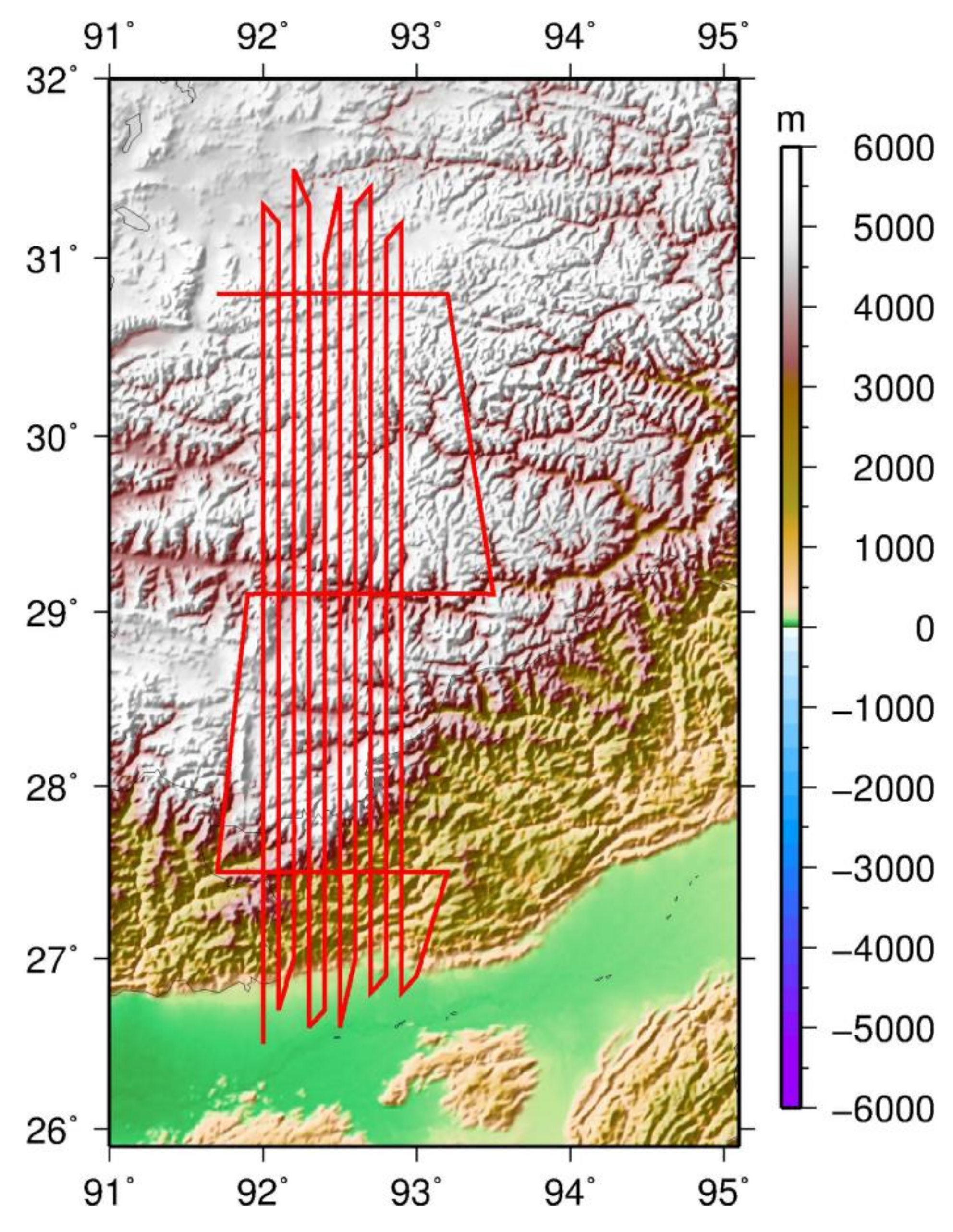
To test the performance of three methods above, a simulation study on the Tibetan Plateau was carried out using gravity data simulated from the global geo-potential model (GGM) EGM2008 [36]. The test area is located from 27°N to 31°N latitude and from 92°E to 93°E longitude. For the study area, where surface gravity data are not available, the airborne gravity anomalies and the ground gravity anomalies were obtained using the EGM2008 from degree/order 360 to 2160. This was enough to roughly approximate the true field, which, nevertheless, was consistent both with the topography and at the flight height. EGM2008 is, of course, not a perfect approximation of the true field for the test region. Gravity anomalies were simulated at 5.5 km and 0 km (sea level) altitudes. Figure 1 shows the distribution of airborne gravimetry lines in the Tibetan Plateau. The simulated error data consist of random and systematic errors. The standard deviation (STD) of the former is 2 mGal, and the latter contains a 3 mGal bias, drift and periodic errors, the rate of drift is 0.002 mGal/s. The frequency of the periodic error is 0.003 Hz, and the amplitude is 6 mGal. The sine function is used to represent the periodic error. The errors in airborne gravimetric surveys can adequately be described as a linear combination of the random error, the bias, the linear drift, and the periodic error. These parameters are obtained based on an analysis of the relationship between the gravity measurement system and systematic errors.

3.1.2. Real Airborne Gravity Data in Taiwan

The Taiwan airborne gravity data was acquired by the National Chiao Tung University [3]. The Taiwan airborne gravimetry was conducted over Taiwan using a LaCoste and Romberg (LCR) System II air-sea gravimeter equipped with a with global positioning system (GPS) data sampled at 1 Hz [3]. This gravimeter has a nominal resolution of 0.01 mGal and an accuracy of better than 1 mGal for the gravity observations. There are four different survey lines with respect to four directions (e.g., north–south, east–west, northeast–southwest, and northwest–southeast), which are shown in Figure 2 (provided by Cheinway Hwang through private contact), the limits of which are from 21.7°N to 25.5°N in latitude and from 119.5°E to 122°E in longitude. The numbers of survey lines in the four directions are 64, 22, 10, and 6, respectively. The cross-line spacing is 4.5 km for all survey lines, except the west–east lines, which were spaced at 20 km. The west–east lines were used mainly for crossover analyses, which reduces the mis-fitting of the observed gravity signal that could be mistakenly considered as colored noise [24]. The cross-line spacing of 4.5 km equals to the theoretical resolvable wavelength of the gravity anomaly at the flight altitude, which was approximately 5156 m. The RMS of crossover differences was 2.88 mGal, corresponding to a 2 mGal STD error in terms of the gravity anomaly.

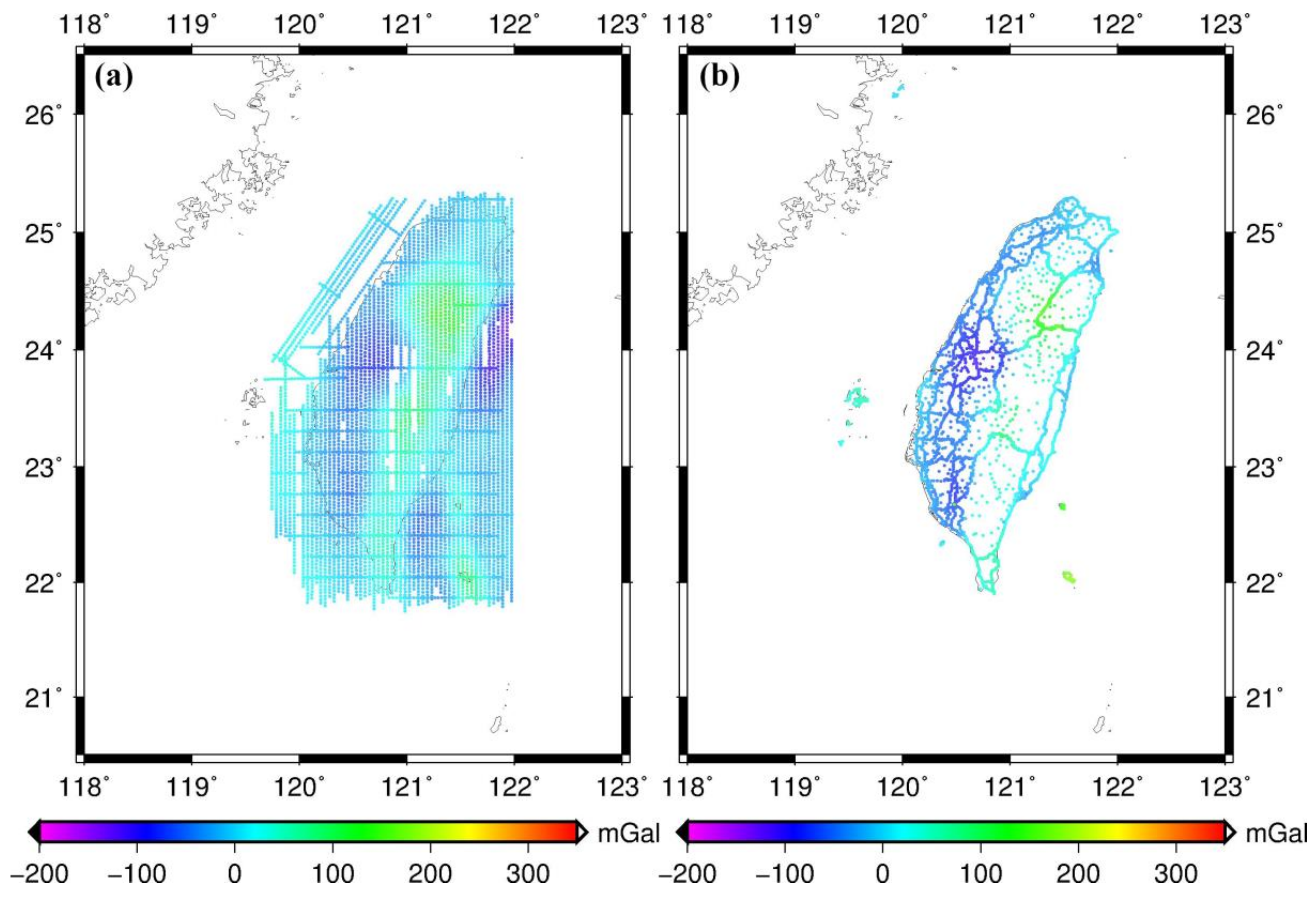
Figure 3 shows the airborne gravity anomalies and land gravity anomalies in Taiwan. The land gravity anomalies were used to validate the airborne downward continuation values. The background of Figure 3 is the topography of Taiwan. According to Figure 3, the maximum values of gravity anomalies are located over the high mountain area. The minimum values are located in the east trench of Taiwan. Visually, the spatial distribution in Figure 3a shows that there is a good fit between the airborne gravity anomalies and the topography of Taiwan. The details of the statistics of airborne gravity anomalies and land gravity anomalies in Taiwan are given in

Table 1. Statistics of airborne gravity anomalies and land gravity anomalies in Taiwan (mGal).

Data Sets	Max	Min	Mean	STD
Airborne gravity anomalies	257.8	−161.1	33.9	64.3
Land gravity anomalies	326.8	−62.6	26.8	67.1

. According to Table 1, the STD of airborne gravity anomalies and land gravity anomalies are 64.3 mGal and 67.1 mGal, respectively, which means that airborne gravity anomalies are smoother than land gravity anomalies.

3.2. Numerical Simulation Test in Tibetan Plateau

In the experiments, we downward continue the gravity anomalies from approximately 5.5 km to 0 km (sea level) based on the three methods described in Section 2. Before LSC is used, the parameters of the covariance function must be estimated. The parameters of LSC in the Tibetan Plateau are determined by GPFIT of GRAVSOFT [27]. For the SPR method, the smoothing parameter is 1.007, and the regularization parameter is 0.504. These parameters are generated by GCV method. The differences between downward continuation values and gravity anomalies are shown in

Table 2. Differences of downward continuation values and gravity anomalies (mGal).

Method	Max	Min	Mean	RMS
The inverse Poisson’s integral	59.8	−44.1	4.4	16.6
The SPR method	56.8	−47.5	−0.1	15.6
The LSC method	50.9	−30.1	4.8	13.2

.

According to Table 2, the inverse Poisson’s integral method yields downward continued gravity anomalies containing larger random and systematic errors because the corresponding STD is the largest one and the mean value is 4.4 mGal. The SPR method is more efficient than the inverse Poisson’s integral. The mean value 4.8 mGal illustrates that the results from LSC are impacted by systematic errors. However, the LSC generates the best result in terms of RMS.

3.3. Downward Continuation of Airborne Gravity Data in Taiwan

The LSC approach can generate the best results in the Tibetan Plateau. The topography of the Tibetan Plateau is as rough as it is in Taiwan. In addition, the inverse Poisson’s integral and the SPR methods are usually applied in grid mode, not in a point-to-point mode [3]. The LSC can downward continue values in point-to-point mode. Therefore, we chose LSC for the downward continuation of airborne gravity in Taiwan. Before the LSC was used, the parameters of the covariance function had to be estimated. The parameters in Taiwan were set according to the parameters fixed by GPFIT from GRAVSOFT [37]. The Satellite only model GO_CONS_GCF_2_DIR_R5 (DIR_R5) [38] was used to remove-restore the long wavelength information in airborne gravity and surface gravity.

To reduce the downward continuation error, we also remove the TC effects in gravity anomalies. According to Forsberg [5], only the short wavelength variations of TC effects is taken into account, which is done by choosing a smooth mean elevation surface, and computationally remove masses above this surface and fill up valleys. This is called the RTM terrain reduction method [5], which is used to compute the short wavelength part of the TC effects in this paper by using the prism integration, and assuming a constant density of 2.67 g/cm³ for all topographic masses. Considering the task of the computations, RTM terrain effects were performed in 0.5° blocks and expanded with 0.3° overlaps. The 30″ × 30″ Shuttle Radar Topography Mission (SRTM) data is used here, and the data processing is same to the one used in [4,6]. After this step, the downward continuation values of airborne gravity in Taiwan are estimated by GPCOL1 in GRAVSOFT [35,37].

The differences between downward continued values and land gravity data are shown in

Table 3. Differences between downward continuation values and land gravity (mGal).

Method	Max	Min	Mean	RMS
The Fourier transform method in [3]	124.7	−146.9	−2.8	19.5
The Fourier transform method removed topographic gravity effect [23]	117.9	−98.1	1.5	18.4
The LSC without TC	84.0	−191.1	−9.6	27.9
The LSC with TC	67.5	−64.0	−1.9	11.7

. The RMS of the differences corresponding to the LSC without TC is 27.881 mGal, and is reduced to 11.653 mGal when TC was applied. Hwang et al. [3] studied the downward continuation using Fourier transform and LSC, and reported that the Fourier transform method delivered the optimal results, which are also shown in the Table 3. The RMS is 18.4 mGal when applying Fourier transform method, which removed the topographic gravity effect [23].

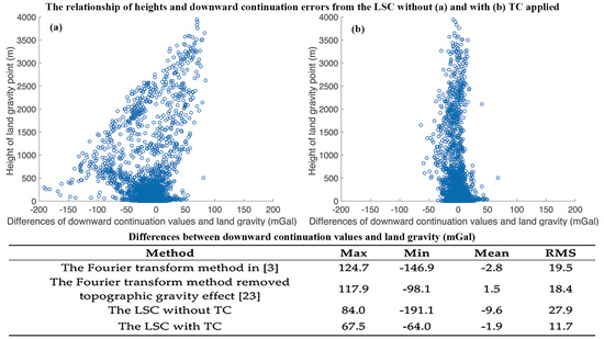
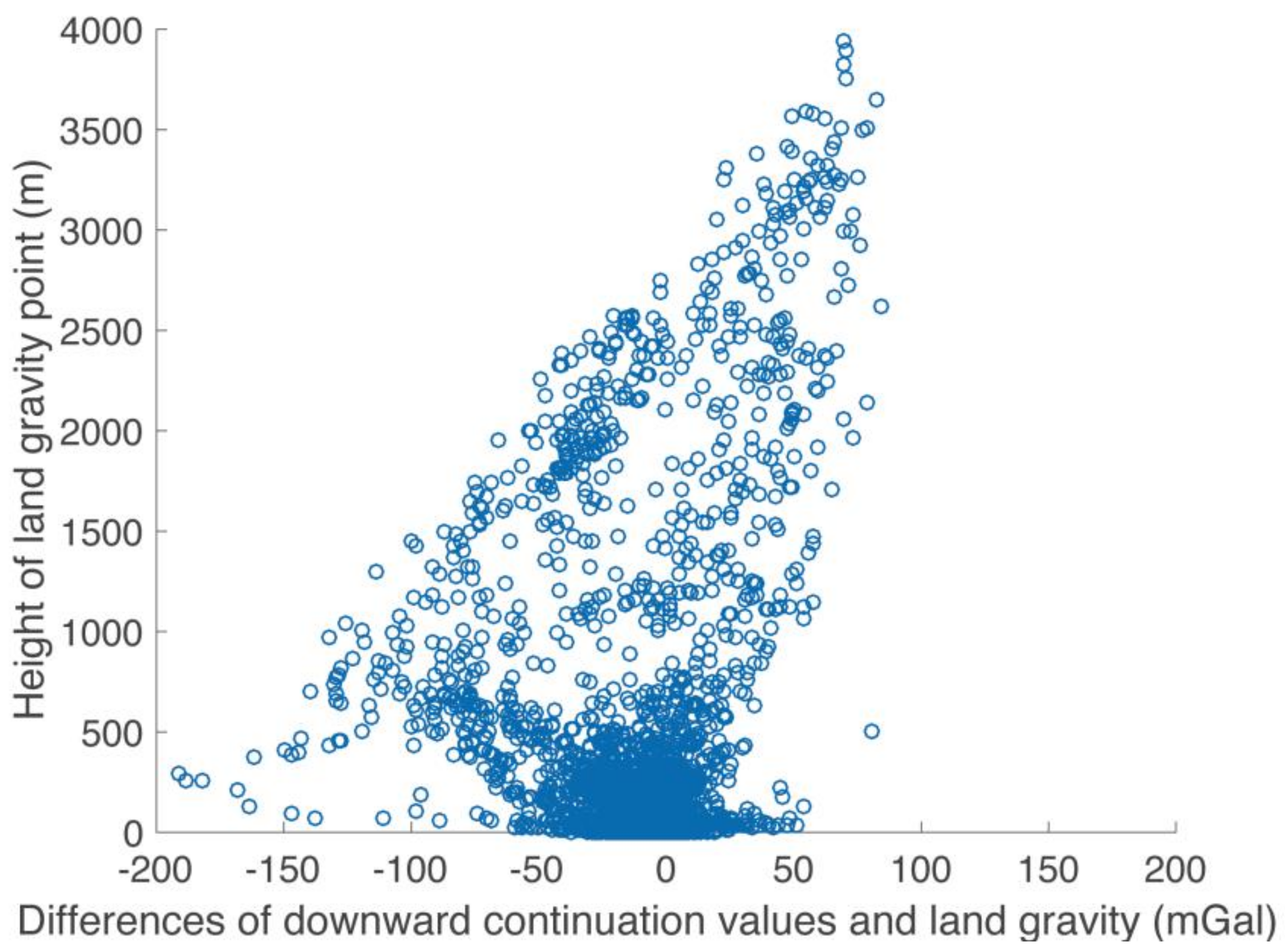
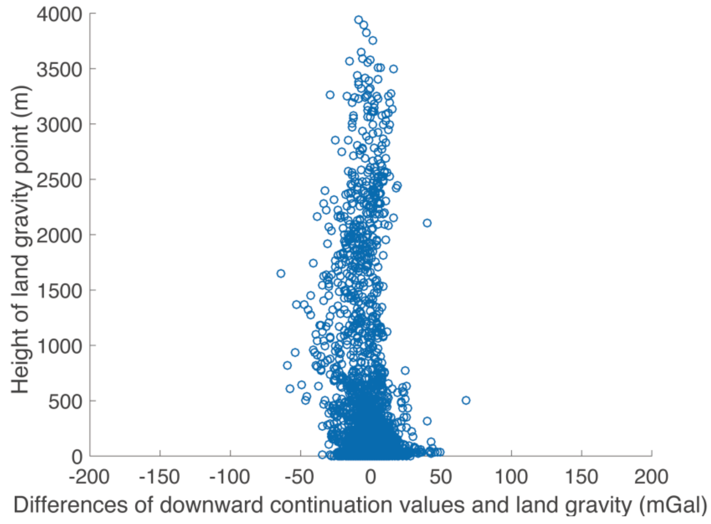
According to Table 3, the improvement of the downward continuation results from LSC is mainly related to the TC effects. Therefore, we analyze the relationship between the heights of land gravity points and the downward continuation errors from the LSC approach with and without the TC applied (see Figure 4 and Figure 5). Figure 4 and Figure 5 reveal the significant changes in the distribution of the points with the help of TC.

3.4. TC Analysis

To illustrate why the TC helps downward continuation, the statistical results of both the airborne gravity anomalies and land gravity anomalies after removing the DIR_R5 model up to d/o 220 degree [38] and the TC effects are reported in

Table 4. Statistics of free-air airborne gravity data and land gravity data after removing GGM and TC (mGal).

Data Sets	Processing Strategies	Max	Min	Mean	STD
Airborne gravity anomalies	Removing GGM	165.7	−131.4	−0.4	44.2
	Removing GGM and TC	137.8	−128.1	−0.7	39.0
Land gravity anomalies	Removing GGM	234.2	−141.7	−21.7	59.6
	Removing GGM and TC	187.5	−122.3	−6.1	53.7

and shown Figure 6. According to Table 4, the Max/Min/Mean/STD values before and after removing the effects of the GGM and TC are of the same order of magnitude but lower in value. Compared with the values in Table 1, after removing GGM, the STD of the free-air airborne and land gravity anomalies reduced from 64.3 mGal and 67.1 mGal to 59.6 mGal and 44.2 mGal, respectively. After removing GGM and TC, the STD of the free-air airborne and land gravity anomalies reduce to 39.0 mGal and 53.7 mGal, respectively. Because the high frequency contribution from the residual terrain can be removed in the remove-compute-restore procedure by RTM method, the STD of airborne gravity anomalies reduces from 44.2 to 39.0 mGal after removing TC [2,4,5]. According to Figure 6, the spatial pattern of free-air anomalies after removing GGM and TC is smoother than that in Figure 3. Figure 7 shows the terrain and bathymetry around Taiwan.

4. Discussion

According to Table 3, the RMS of the LSC method is reduced by more than one half after removing the TC effects computed by RTM method. Compared with Figure 5, the distribution of the points in Figure 4 is more dispersed and shows a tilted feature, especially for the points with heights higher than 500 m. The most significant improvement is that the maximum error reduces from 191.1 mGal in Figure 4 to 67.5 mGal in Figure 5. The big improvement shows that removing TC effects in the complex terrain region is very effective for the LSC method on the one hand, and about 3/4 of downward continuation errors are caused by residual terrain effects on the other hand. Moreover, the LSC method with TC improves the accuracy of downward continuation by approximately 40% compared with the optimal method in [3,23]. Additionally, the improvement indicated in Table 3 and Figure 5 also shows that using the RTM method to compute terrain effects is very effective [2,4,5,6].

Generally, TC effects in the mountainous areas are larger than those in the low elevation areas. Therefore, after removing the TC effects, the spatial pattern of gravity anomalies will become smoother than before. According to Table 4, the airborne gravity anomalies are nicely smoothed by removing the GGM and the TC. Over 75% of Taiwan’s topography is hills and high mountains. The variation of topography over Taiwan and its adjacent ocean area is large, ranging from approximately −6000 m in the trench east of Taiwan to approximately 4000 m in the Central Range of Taiwan. Because the complex topography contributes greatly to the high-frequency part of the gravity anomalies [4,5,6], after removing the TC, the spatial pattern of gravity anomalies in Taiwan in Figure 6 is smoother than the one in Figure 3. The smoother gravity anomalies are more suitable for executing reliable gravity functional computations [26] in general, and for performing a better downward continuation of gravity anomaly signals based on the LSC method [2,4,5,6].

5. Conclusions

To obtain the optimal results of downward continuation in Taiwan, we analyzed the theoretical equations of the three downward continuation methods explained in Section 2. In the experiment step, we conducted comparison tests in the Tibetan Plateau, which showed that the least-squares collocation method generates the best results compared to the inverse Poisson’s integral and the semi-parametric method combined with the regularization method.

We applied the least-squares collocation method with a terrain correction to the downward continuation of real airborne gravity data in Taiwan. The terrain correction was accounted for by the residual terrain modeling approach. The downward continuation results show that, with the help of terrain correction, the RMS of the differences between downward continuation values and land gravity values is 11.7 mGal in this paper. An improvement of approximately 40% was gained compared with the results given by Hwang et al. [3] and Hsiao and Hwang [23]. For the airborne gravity data in the region with complex topography, the terrain correction must be considered in the downward continuation. After removing the terrain correction effects, the magnitude of gravity anomalies decreases and its spatial pattern becomes smoother, which contribute greatly to reducing error in downward continuation. In the future, for further improvement in the downward continuation of airborne gravity, the influences of underwater topography, and more accurate and high-resolution topography data should be considered in data processing. Moreover, some new methods could be tested, such as radial basis functions, machine learning, and etc.

References

- Zhao, Q.; Strykowski, G.; Li, J.; Pan, X.; Xu, X. Evaluation and Comparison of the Processing Methods of Airborne Gravimetry Concerning the Errors Effects on Downward Continuation Results: Case Studies in Louisiana (USA) and the Tibetan Plateau (China). Sensors 2017, 17, 1205. [Google Scholar] [CrossRef] [PubMed]
- Forsberg, R.; Olesen, A.V.; Alshamsi, A.; Gidskehaug, A.; Ses, S.; Kadir, M.; Peter, B. Airborne Gravimetry Survey for the Marine Area of the United Arab Emirates. Mar. Geod. 2012, 35, 221–232. [Google Scholar] [CrossRef]
- Hwang, C.; Hsiao, Y.S.; Shih, H.C.; Yang, M.; Chen, K.H.; Forsberg, R.; Olesen, A.V. Geodetic and geophysical results from a Taiwan airborne gravity survey: Data reduction and accuracy assessment. J. Geophys. Res. Solid Earth. 2007, 112, B04407. [Google Scholar] [CrossRef]
- Forsberg, R.; Olesen, A.; Munkhtsetseg, D.; Amarzaya, B. Downward Continuation and Geoid Determination in Mongolia from Airborne and Surface Gravimetry and SRTM Topography. In Proceedings of the 2007 International Forum on Strategic Technology, Ulaanbaatar, Mongolia, 3–6 October 2007; pp. 470–475. [Google Scholar]
- Forsberg, R. A Study of Terrain Reductions, Density Anomalies and Geophysical Inversion Methods in Gravity Field Modelling; Report 355; Department of Geodetic Science and Surveying, The Ohio State University: Columbus, OH, USA, 1984. [Google Scholar]
- Forsberg, R.; Olesen, A.; Bastos, L.; Gidskehaug, A.; Meyer, U.; Timmen, L. Airborne geoid determination. Earth Planets Space 2000, 52, 863–866. [Google Scholar] [CrossRef] [Green Version]
- Wei, M.; Schwarz, K.P. Flight test results from a strapdown airborne gravity system. J. Geod. 1998, 72, 323–332. [Google Scholar] [CrossRef]
- Bell, R.E.; Blankenship, D.D.; Finn, C.A.; Morse, D.L.; Scambos, T.A.; Brozena, J.M.; Hodge, S.M. Influence of subglacial geology on the onset of a West Antarctic ice stream from aerogeophysical observations. Nature 1998, 394, 58–62. [Google Scholar] [CrossRef]
- Schwarz, K.; Li, Y.C. What can airborne gravimetry contribute to geoid determination? J. Geophys. Res. Solid Earth 1996, 101, 17873–17881. [Google Scholar] [CrossRef]
- Brozena, J.M. A Preliminary-Analysis of the Nrl Airborne Gravimetry System. Geophysics 1984, 49, 1060–1069. [Google Scholar] [CrossRef]
- Barzaghi, R.; Albertella, A.; Carrion, D.; Barthelmes, F.; Petrovic, S.; Scheinert, M. Testing Airborne Gravity Data in the Large-Scale Area of Italy and Adjacent Seas. Acta Oto-laryngol. Suppl. 2015, 532, 77–82. [Google Scholar]
- Wang, Y.M.; Becker, C.; Mader, G.; Martin, D.; Li, X.; Jiang, T.; Breidenbach, S.; Geoghegan, C.; Winester, D.; Guillaume, S.; et al. The geoid slope validation survey 2014 and grav-d airborne gravity enhanced geoid comparison results in iowa. J. Geod. 2017, 91, 1261–1276. [Google Scholar] [CrossRef]
- Mccubbine, J.C.; Amos, M.J.; Tontini, F.C.; Smith, E.; Winefied, R.; Stagpoole, V.; Featherstone, W.E. The new zealand gravimetric quasigeoid model 2017 that incorporates nationwide airborne gravimetry. J. Geod. 2017, 92, 923–937. [Google Scholar] [CrossRef]
- Lu, B.; Barthelmes, F.; Petrovic, S.; Förste, C.; Flechtner, F.; Luo, Z.; He, K.; Li, M. Airborne gravimetry of geohalo mission: Data processing and gravity field modeling. J. Geophys. Res. Solid Earth 2017, 122, 10586–10604. [Google Scholar] [CrossRef]
- Alberts, B.; Klees, R. A comparison of methods for the inversion of airborne gravity data. J. Geod. 2004, 78, 55–65. [Google Scholar] [CrossRef]
- Novak, P.; Kern, M.; Schwarz, K.P. Numerical studies on the harmonic downward continuation of band-limited airborne gravity. Stud. Geophys. Geod. 2001, 45, 327–345. [Google Scholar] [CrossRef]
- Martinec, Z. Stability investigations of a discrete downward continuation problem for geoid determination in the Canadian Rocky Mountains. J. Geod. 1996, 70, 805–828. [Google Scholar] [CrossRef]
- Novak, P.; Heck, B. Downward continuation and geoid determination based on band-limited airborne gravity data. J. Geod. 2002, 76, 269–278. [Google Scholar] [CrossRef]
- Hofmann-Wellenhof, B.; Moritz, H. Physical Geodesy; Springer Science & Business Media: Berlin, Germany, 2006. [Google Scholar]
- Bell, R.E.; Childers, V.A.; Arko, R.A.; Blankenship, D.D.; Brozena, J.M. Airborne gravity and precise positioning for geologic applications. J. Geophys. Res. Solid Earth 1999, 104, 15281–15292. [Google Scholar] [CrossRef] [Green Version]
- Vaníček, P.; Novák, P.; Sheng, M.; Kingdon, R.; Janák, J.; Foroughi, I.; Martinec, Z.; Santos, M. Does poisson’s downward continuation give physically meaningful results? Stud. Geophys. Geod. 2017, 61, 412–428. [Google Scholar] [CrossRef]
- Zhang, C.; Lü, Q.; Yan, J.; Qi, G. Numerical solutions of the mean-value theorem: New methods for downward continuation of potential fields. Geophys. Res. Lett. 2018, 45, 3461–3470. [Google Scholar] [CrossRef]
- Hsiao, Y.; Hwang, C. Topography-assisted downward continuation of airborne gravity: An application for geoid determination in Taiwan. Terr. Atmos. Ocean. 2010, 21, 627–637. [Google Scholar] [CrossRef]
- Braitenberg, C.; Sampietro, D.; Pivetta, T.; Zuliani, D.; Barbagallo, A.; Fabris, P.; Rossi, L.; Fabbri, J.; Mansi, A.H. Gravity for Detecting Caves: Airborne and Terrestrial Simulations Based on a Comprehensive Karstic Cave Benchmark. Pure Appl. Geophys. 2016, 173, 1–22. [Google Scholar] [CrossRef]
- Fessler, J.A. Nonparametric Fixed-Interval Smoothing of Nonlinear Vector-Valued Measurements. IEEE Trans. Signal Proces. 1991, 39, 907–913. [Google Scholar] [CrossRef]
- Fessler, J.A. Nonparametric Fixed-Interval Smoothing with Vector Splines. IEEE Trans. Signal Proces. 1991, 39, 852–859. [Google Scholar] [CrossRef]
- Green, P.J. Penalized likelihood for general semi-parametric regression models. Int. Stat. Rev. 1987, 245–259. [Google Scholar] [CrossRef]
- Engle, R.F.; Granger, C.W.J.; Rice, J.; Weiss, A. Semiparametric Estimates of the Relation between Weather and Electricity Sales. J. Am. Stat. Assoc. 1986, 81, 310–320. [Google Scholar] [CrossRef]
- Rice, J.; Rosenblatt, M. Smoothing splines: Regression, derivatives and deconvolution. Ann. Stat. 1983, 141–156. [Google Scholar] [CrossRef]
- Rice, J.; Rosenblatt, M. Integrated mean squared error of a smoothing spline. J. Approx. Theory 1981, 33, 353–369. [Google Scholar] [CrossRef]
- Wahba, G. Smoothing noisy data with spline functions. Numer. Math. 1975, 24, 383–393. [Google Scholar] [CrossRef]
- Reinsch, C.H. Smoothing by spline functions. Numer. Math. 1967, 10, 177–183. [Google Scholar] [CrossRef]
- Schoenberg, I.J. Spline functions and the problem of graduation. Proc. Natl. Acad. Sci. USA 1964, 52, 947–950. [Google Scholar] [CrossRef] [PubMed]
- Whittaker, E.T. On a new method of graduation. Proc. Edinb. Math. Soc. 1922, 41, 63–75. [Google Scholar]
- Forsberg, R. A new covariance model for inertial gravimetry and gradiometry. J. Geophys. Res. Solid Earth 1987, 92, 1305–1310. [Google Scholar] [CrossRef]
- Pavlis, N.K.; Holmes, S.A.; Kenyon, S.C.; Factor, J.K. The development and evaluation of the Earth Gravitational Model 2008 (EGM2008). J. Geophys. Res. Solid Earth 2012, 117, B04406. [Google Scholar] [CrossRef]
- Forsberg, R.; Tscherning, C.C. An overview manual for the GRAVSOFT Geodetic Gravity Field Modelling Programs. Available online: https://www.academia.edu/9206363/An_overview_manual_for_the_ GRAVSOFT_Geodetic_Gravity_Field _Modelling_Programs?auto=download (accessed on 10 July 2018).
- Bruinsma, S.L.; Förste, C.; Abrikosov, O.; Lemoine, J.; Marty, J.; Mulet, S.; Rio, M.; Bonvalot, S. ESA’s satellite-only gravity field model via the direct approach based on all GOCE data. Geophys. Res. Lett. 2014, 41, 7508–7514. [Google Scholar] [CrossRef]
Figure 1.
Airborne gravimetry lines (red lines) projected on a topographic map of the Tibetan Plateau.
Figure 2.
Taiwan airborne gravimetry lines at a 5156 m flight altitude.
Figure 3.
(a) Airborne gravity anomalies and (b) land gravity anomalies in Taiwan.
Figure 4.
The relationship of heights and downward continuation errors from the LSC without TC applied.
Figure 5.
The relationship of heights and downward continuation errors from the LSC with TC applied.
Figure 6.
Free-air gravity anomalies after removing GGM and TC in Taiwan. (a) Airborne gravity at a height of 5156 m; (b) land gravity on the ground (unit: mGal).
Figure 7.
Terrain and bathymetry around Taiwan.