Defining a Trade-off Between Spatial and Temporal Resolution of a Geosynchronous SAR Mission for Soil Moisture Monitoring


1
Department of Information Engineering, Electronics and Telecommunications, Sapienza University of Rome, 00184 Rome, Italy
2
CIMA Research Foundation, 17100 Savona, Italy
3
Department of Informatics, Bioengineering, Robotics and Systems Engineering, University of Genoa, 16145 Genoa, Italy
*
Author to whom correspondence should be addressed.
Remote Sens. 2018, 10(12), 1950; https://doi.org/10.3390/rs10121950
Submission received: 6 October 2018
/
Revised: 27 November 2018
/
Accepted: 30 November 2018
/
Published: 4 December 2018
(This article belongs to the Special Issue Soil Moisture Remote Sensing Across Scales)
Abstract
:The next generation of synthetic aperture radar (SAR) systems could foresee satellite missions based on a geosynchronous orbit (GEO SAR). These systems are able to provide radar images with an unprecedented combination of spatial (≤1 km) and temporal (≤12 h) resolutions. This paper investigates the GEO SAR potentialities for soil moisture (SM) mapping finalized to hydrological applications, and defines the best compromise, in terms of image spatio-temporal resolution, for SM monitoring. A synthetic soil moisture–data assimilation (SM-DA) experiment was thus set up to evaluate the impact of the hydrological assimilation of different GEO SAR-like SM products, characterized by diverse spatio-temporal resolutions. The experiment was also designed to understand if GEO SAR-like SM maps could provide an added value with respect to SM products retrieved from SAR images acquired from satellites flying on a quasi-polar orbit, like Sentinel-1 (POLAR SAR). Findings showed that GEO SAR systems provide a valuable contribution for hydrological applications, especially if the possibility to generate many sub-daily observations is sacrificed in favor of higher spatial resolution. In the experiment, it was found that the assimilation of two GEO SAR-like observations a day, with a spatial resolution of 100 m, maximized the performances of the hydrological predictions, for both streamflow and SM state forecasts. Such improvements of the model performances were found to be 45% higher than the ones obtained by assimilating POLAR SAR-like SM maps.
1. Introduction
Within the Earth system science framework, soil moisture (SM) represents a key variable because it directly controls water and energy fluxes between the atmosphere and the land surface [1,2,3]. For this reason, its accurate monitoring is fundamental to a plethora of applications, such as meteorology, agriculture (e.g., irrigation management), hydrology and weather-related risk assessment and forecasting (e.g., floods, landslide, drought) [2,3,4,5,6]. From this list, the focus of this paper is on hydrological applications (e.g., hydrological modelling and discharge prediction).
The challenge of SM monitoring comes from its high variability, both in space and in time [3]. Such variability depends on the complex interaction of different environmental factors (e.g., soil properties such as texture and structure, topography, vegetation, radiation, precipitation, evapotranspiration, groundwater) that also change in space and in time [2,3,7]. Concerning hydrological applications, the scientific community pointed out the need for a more accurate strategy for SM monitoring at higher spatio-temporal resolutions [3,8].
Amongst the different techniques for SM monitoring, networks of in situ monitoring stations are able to provide accurate and continuous data at different soil depths. Therefore, they are particularly suitable for characterizing temporal trends. However, such networks are often scarce and not fairly distributed, and are not fully representative of SM spatial patterns [1,9,10,11,12]. This can be a strong limitation for operational applications where SM data are required, for instance those related to operational hydrology.
Synoptic, large-scale surface SM estimates are provided by remotely sensed data, such as those acquired by Earth Observation (EO) spacecraft. Although optical and thermal sensors can be used for such purposes, microwave remote sensing is particularly suitable for monitoring SM because it exploits the direct relationship between water content and the soil dielectric constant. In any case, sensors and satellite mission characteristics constrain the spatio-temporal sampling of SM products. Moreover, SM retrievals from microwave sensors refer to the subsurface soil layer (<10 cm), because the penetration depth is inversely related to the sensor’s frequency [5,8,10,12]. Most of the microwave space missions currently used for SM monitoring exploit scatterometer (the advanced scatterometer—ASCAT: C-band) and radiometer sensor data (advanced microwave scanning radiometer 2—AMSR2: C and X-band, soil moisture and ocean salinity—SMOS: L-band, soil moisture active passive—SMAP: L-band). Their observations are characterized by low spatial resolution (SpR) —about 25-50 km—and high temporal resolution (TeR)—approximately 1–3 days [3]. Since the launch of the Sentinel 1 (S1) constellation (2014), composed of two satellites (S1-A and S1-B) which carry a C-band synthetic aperture radar (SAR) sensor, the scientific community has begun to investigate the potential for operational SM monitoring at high SpR (0.1–1 km) and moderate TeR (≤6 days) [13,14,15,16];also for hydrological applications [17,18,19,20,21,22]. Hence, with current technologies, there is a lack of satellite-derived SM observations with sub-daily revisit time and high SpR. For these reasons, efforts have been made by the scientific community to combine different satellite-based SM estimates and develop enhanced downscaling techniques for improving SpR, or methods for merging different datasets to increase the TeR [2,23,24]. In this respect, a SAR sensor aboard a satellite platform placed on a geosynchronous orbit—so called geosynchronous synthetic aperture radar (GEO SAR)—can combine the short revisit time of the platform and the high SpR of the radar sensor. The feasibility of such a mission was demonstrated by previous studies [25,26,27], and this paper was intended to assess its impact on hydrological applications [28].
SM can also be evaluated by numerical (e.g., hydrological or land surface) models, which are able to represent the catchment state at a desired (e.g., high) spatial and temporal resolution. Furthermore, they are able to model SM at different depths, according to the physical processes they implement. However, modelling errors (e.g., model initialization, parameterization, approximations in the representation of the physical processes, uncertainties in the meteorological inputs, etc.) may reduce the quality of such estimates [5,29]. In addition, some relevant processes have anthropic origin, such as irrigation or dam interception, and are difficult to parameterize [8].
A method able to obtain SM estimates with higher level of accuracy is via data assimilation (DA). These techniques allow to optimally combine external observations (e.g., satellite-based SM estimates) with numerical models (e.g., hydrological models) with different spatio-temporal resolutions, by properly accounting for their uncertainties [29,30,31]. Several studies have been carried out in recent years to show the potential of soil moisture data assimilation (SM-DA), including References [17,18,19,20,21,32,33,34,35,36,37,38,39] amongst others. Nonetheless, SM-DA is not a trivial concept and encompasses different aspects. As such, it has been studied and analyzed according to different perspectives. The main issues concern the choice of the best sensor/space mission (e.g., their frequency, revisit time, SpR, operation mode) [10,40], the choice of SM retrieval algorithm [10,12,41,42,43], and the definition of the DA algorithm [29,30,31,44]. However, there exist other problems, related to the different nature of the observed and modelled data, that must be handled in a SM-DA system [10,35,45,46,47]. In particular, as already described, microwave radiometers and scatterometers have spatial resolutions too coarse for catchment scale applications, and refer to the near-surface soil layer, with a depth in the order of few centimeters, while the moisture of the soil layer mostly used for hydrological applications is that of the root zone (RZ), with a depth of up to 1–2 m [48]. These differences may produce systematic errors (biases) between modelled and observed data, and must be removed when assimilation strategies aim at correcting zero-mean random errors [10,46,49,50,51,52,53]. Despite noteworthy efforts that have been made to develop bias correction techniques [45,46,47,54], systematic errors are unlikely to be fully removed and their effects can be observed in the SM-DA final product [53]. Finally, the issue of error characterization of both modelled and observed data must also be addressed in a SM-DA system [35].
Bearing in mind the above-mentioned framework, the research presented in this work aimed at investigating the potential of a GEO SAR satellite mission concept for hydrological applications [25,27]. In particular, it assessed the potential utility of simulated GEO SAR SM data in a SM-DA system. For this purpose, different GEO SAR observation configurations, in terms of spatial and temporal resolution, were explored. Moreover, this utility was evaluated in comparison to that of currently operating SAR instruments carried by satellites flying on a quasi-polar orbit (POLAR SAR).
A GEO SAR mission named Geosynchronous—Continental Land-Atmosphere Sensing System (G-CLASS) has been recently proposed to the European Space Agency (ESA), in response to the call for a future Earth Explorer satellites (EE-10). Unlike the satellite missions currently used for SM monitoring (which fly on a quasi-polar orbit), the geosynchronous orbit of a GEO SAR platform could observe SM dynamics with both high SpR (≤1 km) and high TeR (≤12 h). Such spatio-temporal resolutions are actually not achievable by means of existing satellites, which are not able to fully capture SM dynamics either in the spatial or the temporal domain [24]. The spatio-temporal resolution of the GEO SAR sensor is achieved thanks to a geosynchronous elliptic orbit, which enables the system to move eastward and then westward with respect to the Earth during the day, and thus to build up a synthetic antenna. According to the length of the antenna focused on the ground, images can be generated with different time sampling and, accordingly, different SpR. C-band is presently envisaged as a compromise between SM detection capability and system performances for the G-CLASS mission, but this is not relevant for the purpose of this study, where the focus is on the spatio-temporal resolution of SM observations [28]. As GEO SAR SM maps could be produced with diverse SpR and TeR, the objective of this work was to define which combinations could be most useful for hydrological applications. Although previous studies have been carried out to define the requirements of a global near-surface soil moisture satellite mission in terms of accuracy, repeat time, SpR [40], and specifying quantitative user requirements for different applications (including hydrology) [55], in literature there is a lack of similar studies specifically designed for a GEO SAR sensor.
In this study, the above-mentioned investigation was carried out by setting up a synthetic twin SM-DA experiment, where a ‘reference’ model simulation (the outcome of which is assumed to be the ’truth’) was compared against a set of perturbed model simulations, obtained in a SM-DA framework, that represent a realistic context of hydrological simulations. In the experiment, SM observations characterized by diverse spatio-temporal resolutions and accuracy, compliant with the one potentially achievable by the GEO SAR sensor (and thus hereinafter defined, for the sake of the simplicity, as GEO SAR-like SM products), were produced, starting from the SM maps of the ‘reference’ model simulation. The latter were then assimilated into the perturbed SM-DA modelling framework, to observe the impact on streamflow simulations and modelled SM state estimates. Since the methodological approach that was developed did not address the issue of SM retrieval from GEO SAR images, this paper does not implement and discuss any simulation of the acquisition chain of the instruments. Instead, it aims at identifying the best compromise between the spatial and the temporal resolution of SM products potentially delivered by a SAR sensor, including the GEO SAR.
To understand if GEO SAR-like SM products can provide an added value with respect to the SM products derived from existing SARs (such as S1) in the SM-DA framework, the experiment was complemented by an analogous investigation in which the SM observations were simulated (always starting from the SM maps of the ‘reference’ model simulation) as they were produced by a POLAR SAR system, like the S1 constellation. Such observations (that will be hereinafter defined POLAR SAR-like SM products) were produced to have a TeR equal to S1 data, and a SpR equal to that of the GEO SAR. POLAR SAR-like SM products were then assimilated in the previous SM-DA system, and the results compared against those obtained with the GEO SAR synthetic products.
The paper is organized as follows: the study area is described in paragraph 2.1, whereas the data and the hydrological model that were used in the experiment are depicted in paragraph 2.2 (Section 2). In Section 3, the description of the assimilation algorithm (paragraph 3.1) and the explanation of the experiment design (paragraph 3.2) are presented. The results of the experiment are then shown in Section 4 and discussed in Section 5. Finally, the conclusions of the study are drawn in Section 6. A table summarizing the acronyms used in the paper can be found in the back matter.
2. Study Area and Materials
2.1. Study Area
In order to carry out the synthetic experiment in a realistic scenario, the SM-DA system was implemented at catchment scale in a real basin: the Cervaro River Catchment (Southern Italy). The selected hydrological basin has a surface area of ca. 760 km2 and the river length is ca. 100 km. The catchment includes areas of the provinces of Avellino (Campania Region) and Foggia (Puglia Region), stretching from south-west to north-east. The river originates from the Subappennino Dauno, crosses the Tavoliere delle Puglie plain, and flows into the Adriatic Sea (Figure 1). The basin has a semi-arid Mediterranean climate, characterized by short temperate winters, where the majority of rainy events occur, and hot, dry summers. Average annual temperature ranges between 15 °C and 17 °C. The rainfall pattern is variable: it is higher in the upstream portion of the basin (average annual precipitation ca. 1000 mm), whereas it is lower in the downstream portion of the catchment (average annual precipitation ca. 400 mm) [56]. The basin was selected because it has optimal conditions for SM retrieval from SAR acquisitions, i.e., predominant flat topography, low percentage of areas covered by urban settlements and forests [20] (Figure 2).
2.2. Data and Hydrological Model
The numerical model exploited for the experiments was Continuum, which is a time-continuous, spatially-distributed and physically-based hydrological model [58,59]. The model is currently used in Italy by the Italian Civil Protection Department (DPC) for civil protection applications (e.g., flood/flash flood forecasts), both at national and regional scale. Continuum has six parameters that must be calibrated: two for the surface flow (friction coefficient in channels: Uc; flow motion coefficient in hillslopes: Uh), two for the sub-surface flow (mean field capacity: Ct; infiltration capacity at saturation: Cf), and two for deep flow and the water table (maximum water capacity of the aquifer on the whole investigated area: VWmax; anisotropy between the vertical and horizontal saturated conductivity and soil porosity: Rf). For the ‘reference’ run of the synthetic SM-DA experiment, the calibration parameters operatively used in Italy by DPC for the national implementation of the model were used (Uc = 20; Uh = 0.6; Ct = 0.47; Cf = 0.052; VWmax = 1000; Rf = 5). The latter were obtained by adopting a standard calibration approach aimed at minimizing the differences between modelled and observed discharge data (although a study describing the calibration of the model at national scale has not been published, the reader can refer to Reference [58] for an exemplifying description of such a calibration strategy exploited for Continuum).
For the purposes of the present study, it is important to describe how the SM is modelled by Continuum. In the model configuration, the SM state variable is expressed in term of saturation degree (SD), and refers to the RZ (RZ-SD). More precisely, in Continuum the RZ-SD corresponds to the ratio between the actual soil water content of each cell ( [mm], computed every time-step t) and its maximum storage capacity ( [mm], the average value of which is 155 mm at catchment scale). Therefore, RZ-SD is a dimensionless variable [-], which can have values ranging between 0 and 1. For a detailed description of the model, please refer to References [58,59].
In this experiment, all the model realizations were run with a SpR of 100 m and a TeR of 1 h. The time period investigated in the experiment ranged from 1 October 2016 00:00 to 31 January 2017 23:00 (corresponding to a total of 2952 h). This period was selected as representative of winter months in which—in the selected study areas—rainy events that can potentially generate floods/flash floods are likely to occur. Additionally, it is important to highlight that, for the selected period, there were available S1 data acquired by the two satellites composing the S1 constellation: S1-A and S1-B. The acquisition times of both satellites were used to define the TeR of the simulated POLAR SAR-like SM products (see paragraph 3.2 for further details).
The network of in situ meteorological stations of the Regional Functional Centre for Civil Protection activities of Puglia Region provided the meteorological inputs required by the model: precipitation, temperature, air humidity, electromagnetic radiation (shortwave infrared), and wind speed. All these data, except precipitation, were spatially interpolated to produce hourly maps of meteorological forcing. The interpolation algorithms were: inverse distance weighting (IDW), corrected with a linear regression for accounting the height effect for air temperature, and IDW for the other parameters. Concerning precipitation, rainfall data were not directly interpolated. To produce more realistic precipitation maps, the recorded rainfall volume was exploited to simulate a new precipitation field at high resolution (SpR 100 m; TeR 1 h), to be used in the ‘reference’ run of the experiment. These maps were obtained by means of the Rainfall Filtered Autoregressive Model (RainFARM), which is a model able to downscale a rainfall precipitation field to a finer scale by preserving the original statistical properties [60]. Therefore, the newly generated RainFARM precipitation field preserved, in each (hourly) time step, the original rainfall volume recorded by the pluviometers. However, the volume of rain was randomly redistributed in space, in order to simulate the spatial structure of possible ‘realistic’ precipitation events that may have generated it.
3. Method
3.1. Assimilation Algorithm
The assimilation algorithm used in the SM-DA experiment was the Nudging (Equation (1), [29,44]). In the Nudging (or Newtonian Relaxation) approach, a term is added to the prognostic model equations to gradually relax the solution towards the observations. The nnovation is defined as the difference between the observation (XOBS) and the model forecast (XMOD). The latter is updated every time step (t) an observation is available.
In Equation (1), the superscripts ‘−’ and ‘+’ refer to the time before and after the update, respectively. H is the observation operator that maps the observations into the model space. G is the gain, which acts as a weighting factor for the innovation. The gain depends on the error of the modelled and observed data. In its scalar form, G ranges from 0 to 1. If G is equal to 0, the observation is not taken into account during the analysis step (open loop—OL—mode); if G = 1 the observation replaces the model forecast (direct insertion—DI—mode). Different approaches can be exploited to quantify G, however, normally it is a constant value in both space and time. In this exercise, different G values, ranging from 0 (OL) to 1 (DI) with step of 0.2, were used during the SM-DA experiment to carry out a sensitivity analysis for the G parameter [20,32]. Due to its formulation, the Nudging is an efficient (i.e., computationally inexpensive) assimilation algorithm, useful for operational applications. This is the reason why it was selected for the SM-DA experiments, as well as the fact that several research studies have proven its effectiveness for SM-DA applications (e.g., References [5,20,32,33,38,61] amongst others). It is also important to say that, during the SM-DA experiment, the assimilation was not carried out in river channels, urban areas, and when the modelled land surface temperature (LST) was lower than 0 °C. This temperature can be associated with frozen soil conditions, which are likely to produce inaccurate SM estimates from the radar [62].
3.2. Experiment Design
As previously explained, the objective of this paper was to evaluate the potential and the best configuration (in terms of spatio-temporal resolution) of GEO SAR SM observations for hydrological applications. To this end, a synthetic SM-DA experiment was set up. In the experiment, a ‘reference’ model simulation was compared with a set of perturbed model simulations obtained in a SM-DA system. The ‘reference’ model simulation was assumed to represent the ‘truth’, and hereinafter it is denoted as the TRUTH run. The perturbed simulations (denoted as PERTURBED runs), instead represent how the ‘truth’ is modelled, in a realistic situation, by means of a hydrological model in which satellite SM data are assimilated (GEO SAR-like and POLAR SAR-like, in this case). The experiment is based on the assumption that any attempt to model the truth is imperfect (i.e., affected by different kinds of errors). Thus, the PERTURBED runs were obtained by perturbing the TRUTH run in order to replicate the errors that are common in hydrological modelling. The latter are represented by the error induced by the wrong representation of the precipitation field and the error generated by an incorrect representation of the physical processes. The ‘true’ precipitation field and calibration parameters were thus perturbed, as it will be detailed later on, in order to generate the PERTURBED runs. Please note that when the PERTURBED run of the model does not consider any SM assimilation, it is defined as OL run because, in a Nudging-based assimilation scheme, it corresponds to a run in which the G value is equal to 0.
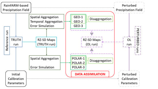
The GEO SAR and the POLAR SAR synthetic SM products were generated by exploiting the SM data obtained from the TRUTH run. To this aim, the latter were impaired by the expected retrieval errors and actual sensor resolutions. Subsequently, they were assimilated in the Nudging-based SM-DA system of the PERTURBED runs to observe the impact of the assimilation on the discharge and SM state variable predictions. In few words, the purpose of the SM-DA experiment was to evaluate if, and to what extent, the assimilation of the GEO SAR-like and the POLAR SAR-like SM products allowed the outputs of the PERTURBED runs to better reproduce the outputs of TRUTH run, with respect to the OL case. A schematic representation of the synthetic SM-DA experiment is shown in Figure 3. A detailed description of the different steps implemented during the experiment is reported hereunder.
- (1)
- Initially, a ‘reference’ model simulation was produced by running the Continuum model using the RainFARM-based high-resolution precipitation field as one of the inputs (this is the TRUTH run). The model calibration parameters were those operatively used by DPC in the national implementation of the Continuum model, and the results were assumed as the ‘truth’.
- (2)
- The TRUTH model settings were then modified (leading to the so-called PERTURBED runs) by using perturbed precipitation fields and calibration parameters. Rainfall data were perturbed by simulating a network of synthetic pluviometers that were randomly and uniformly distributed in the catchment (Figure 4a). The RainFARM-based precipitation field was sampled at the rain gauges location, and the samples were then interpolated using the Kriging algorithm. This approach was adopted to generate a realistic precipitation field, affected by the same errors that very likely occur when interpolating data collected by pluviometers. This often produces an incorrect estimation of rainfall volume (most of the time, the precipitation field is underestimated), as well as an incorrect spatial distribution of the precipitation patterns. Figure 4b shows how the first error was actually simulated in the perturbed precipitation field. In the figure, the time series of the catchment average value of the RainFARM-based precipitation field is compared against the time series of the catchment average value of the perturbed one. In Figure 4c,d, instead, the maps that compare the mean and the maximum values of the two precipitation fields are reported. In addition to the underestimation error (already discussed), these maps show the different rainfall spatial pattern. Since hydrological simulations are also affected by modelling errors, the PERTURBED runs were also executed with a set of slightly different calibration parameters (with respect to the TRUTH run). The latter were obtained by randomly perturbing the two sub-surface flow calibration parameters of Continuum model (i.e., the parameters that are likely to be mostly affected by SM-DA) within their physically admissible range (perturbed calibration parameters: Uc = 20; Uh = 0.6; Ct = 0.42; Cf = 0.057; VWmax = 1000; Rf = 5).
- (3)
- Afterwards, the RZ-SD maps generated by the TRUTH run (hereinafter defined TRUTH SM Maps, and characterized by a SpR of 100 m a TeR of 1 h) were used to simulate the observations collected by the GEO SAR and the POLAR SAR systems.
- (a)
- In order to generate the GEO SAR-like SM products, the TRUTH SM Maps were spatially and temporally aggregated according to the GEO SAR products specifications reported in Table 1. It must be considered that a GEO SAR system is expected to acquire data through two time windows per day of 8 h each, preceded and followed by 2 h without acquisitions. This is because the relative speed of the satellite and the Earth surface is very small at the extreme of the synthetic antenna length, when the satellite goes back to acquire another image. For each time-window, eight GEO-1 images, four GEO-2 images and one GEO-3 image are produced. GEO-1 and GEO-2 were obtained by averaging over 4 × 4 and 8 × 8 pixels of the RZ-SD maps of the TRUTH run (that has a SpR of 100 m), respectively. The results were then divided by the average of the values, computed over the same block of pixels, to obtain the final RZ-SD maps at the desired resolution. This spatial filter was not required to produce GEO-3, which has the same SpR of TRUTH SM maps. Concerning the temporal aggregation, to account for the time required to collect the synthetic antenna, GEO-2 and GEO-3 were obtained by averaging in the temporal domain the values produced by the TRUTH run over a time interval of, respectively, 2 and 8 h. This temporal filter was not required to produce GEO-1, which has the same TeR as the TRUTH SM Maps. After the spatio-temporal aggregation, the three GEO SAR products were perturbed by adding a white Gaussian noise to simulate the expected instrumental/retrieval error [40]. Considering that an error standard deviation of SM in the order of 0.06–0.09 m3/m3 [13,14] is generally expected for SAR retrieval over sparsely vegetated areas, a standard deviation of 0.07 m3/m3 was used in our synthetic experiment. Since the soil of the study area is classified as clay and sandy clay loam [63], an average (and constant) value of porosity equal to 0.45 was used for the whole catchment [64]. Therefore, the SM error of 0.07 m3/m3 translated into a value of 0.156 in terms of SD. Afterwards, the portions of the catchment where the retrieval from a SAR sensor was not feasible were masked out to simulate the actual retrieval capability of a SAR system. The mask was derived by combining the information from the 2012 Corine Land Cover and the SRTM DEM. Following Reference [20], masked pixels correspond to urban areas, forests, water bodies and pixels whose slope is >15°.It must be considered that, amongst the synthetic observations, only the GEO-3 product has a SpR coincident with the one of the Continuum model and, therefore, could be assimilated without further data processing. Concerning the other observations (i.e., the GEO-1, GEO-2, products) a simple disaggregation strategy, based on the proportion shown in Equation (2), was applied to disaggregate them to 100 m before carrying out the assimilation. This step was required for enabling the assimilation of the observations over the model grid space.where represents the SD disaggregated (SpR 100 m) value of each pixel of a GEO SAR map, at a given instant of time ; represents the SD value of each aggregated (SpR 400 m and 800 m) pixel of a GEO SAR map, at a given time instant ; and represent the mean SD values, computed over the investigated period, for each pixel of the OL run with a SpR of, respectively, 100 m, 400 m and 800 m. The maps of the OL run at coarser SpR were generated by applying the same algorithms of spatial aggregation previously described.Example of GEO SAR-like SM maps, before and after the disaggregation process, are shown in Figure 5, as opposed to the corresponding maps of the TRUTH and the OL runs. From the figure it can be observed that, on the one hand, during the generation of the GEO-1 and GEO-2 products, the process of spatial averaging blurred the details of the hydrological network. On the other hand, such details were re-emphasized by the disaggregation process.
- (b)
- Concerning the POLAR SAR-like SM products (hereinafter defined POLAR-1, POLAR-2 and POLAR-3), they were initially produced with a SpR equal to the one of the GEO SAR simulated data (i.e., 800 m, 400 m, 100 m), and a TeR equal to the one of Sentinel 1 constellation. In line with this aim, the real acquisition times of S1-A and S1-B over the Cervaro River Catchment were used to set the TeR of the POLAR SAR observations (Table 2 and Table 3). The hourly TRUTH SM Maps corresponding to the acquisition time of S1 images were thus used for generating the POLAR SAR-like SM products, by applying the same approach used to generate the GEO SAR observations. The only difference was that the temporal aggregation step was not needed (i.e., S1 acquisition can be considered almost ‘instantaneous’), and so the TRUTH SM Maps were only averaged in space and perturbed (with an error standard deviation of 0.07 m3/m3) in order to simulate the instrumental/retrieval error.Subsequently, the POLAR-1 and the POLAR-2 products were disaggregated to 100 m to match the same SpR of the model grid by using the proportion shown in Equation (2).
- (4)
- Finally, the GEO SAR and the POLAR SAR-like SM products (at 100 m SpR) were assimilated into the PERTURBED runs of the Continuum model by using the Nudging assimilation algorithm (Equation (1)). In each time window of 8 h, when the GEO SAR sensor is expected to acquire data, GEO-1 Disaggregated products were assimilated with hourly frequency, whereas GEO-2 Disaggregated and GEO-3 products were assimilated in the middle of the temporal window used for averaging data over time (i.e., 1 h and 4 h after window start for GEO-2 and GEO-3, respectively). The POLAR-1 Disaggregated, POLAR-2 Disaggregated and POLAR-3 products were instead assimilated at the time of the S1 overpass.
It is important to point out that since the SAR-like SM products were simulated directly from the SM of the TRUTH run, they are expressed in terms of SD and are referred to the RZ. In reality, this condition is not feasible because, as explained in the introduction, satellite-based SM observations are only able to monitor the SM of the near-surface soil layer. Moreover, they are usually affected by systematic errors (biases) that must be corrected before the assimilation. In order to understand the impact of only the spatio-temporal resolution of the products in the SM-DA experiment, it was decided to remove from the analysis the uncertainties that would have been derived by simulating near-surface SM observations, i.e., the SAR-like SM products were produced as if they were already bias-corrected.
It is also noteworthy to observe that, as previously explained in the introduction, in real SM-DA system, bias effects are unavoidable and its correction is often not fully successful. Therefore, the slightly different average values (i.e., systematic error) between the TRUTH run, the GEO-1 Disaggregated, GEO-2 Disaggregated and GEO-3 (or POLAR-1 Disaggregated, POLAR-2 Disaggregated and POLAR-3) products, as opposed to the OL run, that can be observed in Figure 6 must be considered as a feature intrinsic to the nature of DA, which is likely to be present in a real SM-DA system. In the experiment, such ‘residual’, uncorrected bias was mostly due to the different precipitation fields used in the OL and TRUTH model simulations (Figure 4). In fact, the interpolated precipitation field used in the OL run (characterized by an underestimation error with respect to the RainFARM precipitation field) generated average RZ-SD values lower (i.e., drier) than the ones of the TRUTH SM Maps. Since the GEO SAR-like SM products were produced from the TRUTH SM Maps, the average RZ-SD values of the OL run are also lower than the average values computed from the GEO SAR data. Following Reference [40] we decided to take advantage of this realistic condition of observations slightly affected by a ‘residual’ bias to study its effect in a SM-DA system.
By observing the Figure 6, it is difficult to understand the differences amongst the different mean satellite-based RZ-SD maps. For this reason, it is worth referring also to Figure 7, which shows the differences between the mean RZ-SD maps of the disaggregated SM products (i.e., GEO-1 Disaggregated, GEO-2 Disaggregated and POLAR-1 Disaggregated, POLAR-2 Disaggregated) and the mean RZ-SD maps of the GEO-3 and POLAR-3 products. From Figure 7 it can be observed that the finer scale products show higher SM values, especially in the areas located nearby the river network where the topography allows higher runoff values.
4. Results
Results of the synthetic experiment were evaluated using two approaches:
- Indirect: by analyzing the impact of the assimilation on model discharge predictions.
- Direct: by analyzing the impact of the assimilation on modelled SM state estimates.
In this context, the adjective ‘indirect’ refers to the evaluation of the effect of the assimilation of the SM maps on another model variable (i.e., discharge predictions). On the other hand, the adjective ‘direct’ refers to the evaluation of the effect of assimilation of the SM maps on the same model variable (i.e., SM state estimates). Although the interpretation of an indirect validation can be complicated by the nonlinear relationships existing between the components of the hydrological cycle, such an approach is commonly used in literature for evaluating the impact of SM-DA (e.g., References [5,20,32,35,37,38] amongst others). This is mostly due to two reasons. On the one hand, there is a higher availability of discharge data with respect to SM measurements. In fact, as previously explained in the introduction, it is difficult to have distributed network stations able to provide accurate in situ SM measurements. Therefore, direct validation strategies can be put in place only in selected areas that—very often—do not correspond to the whole extent of the catchment. On the other hand, developing tools and methods for making more accurate discharge predictions represents a fundamental objective in hydrological applications, e.g., floods and flash floods predictions. Within this framework, comparing the two strategies for assessing the results of the synthetic SM-DA experiments brings an added value in the domain of SM-DA validation.
To validate the results according to the aforementioned approaches, the hourly streamflow forecasts and the RZ-SD values of the PERTURBED model runs before (G = 0, corresponding to the OL run) and after (0 < G ≤ 1), the assimilation were compared against the hourly discharge and the hourly RZ-SD estimates produced by the TRUTH run. Discharge data were evaluated at the Incoronata station (Figure 1), whereas RZ-SD values were evaluated in a distributed way using the RZ-SD maps produced by the model simulations.
Three different performance indexes were used to quantitatively assess the results of the analysis related to streamflow simulations: the Nash-Sutcliffe (NS [-]) efficiency coefficient [65], the efficiency (Eff [%]) of assimilation [35] and the Normalized Error Reduction (NER [%]) [66].
NS (Equation (3)) ranges from −∞ to 1 and the higher its value, the better is the result, i.e., the closer the OL run is to the TRUTH run after SM-DA. Negative values of NS imply that the model is performing worse than using the mean of the observed time series (climatology) as reference for forecasts. A NS value equal to 0, instead, means that the model does not add any information to the climatology. In order to represent NS values in terms of improvement or worsening of the model runs after SM-DA (NSDA) with respect to the OL run (NSOL), NS values were defined in relative terms with respect to the OL run (ΔNS [-]), as in Equation (4). Following Equation (4), positive ΔNS values show an improvement of the model run after SM-DA, whereas negative ΔNS values show a model worsening after SM-DA. It must be pointed out that NS has been widely used in hydrology to evaluate models’ performances, because it is an index useful to assess the overall level of agreement between observed and modelled data. However, because of its formulation, it has some drawbacks: it is biased towards higher flows and insensitive to low(er) values. Furthermore, it is not sensitive to systematic (positive or negative) errors, and it is likely to produce optimistic results if the hydrological regime under investigation shows marked seasonal variations. Therefore, NS interpretation could be difficult to interpret [67,68]. For these reasons, and to avoid ambiguities when interpreting discharge results, two further indexes were used to evaluate them: Eff and NER. Eff (Equation (5)) ranges from −∞ to 100, and represents the percentage of model worsening (Eff < 0) or improvements (Eff > 0) after SM-DA. An Eff value equal to 0 represents neither improvement nor worsening. NER (Equation (6)) is a dimensionless value, ranging between −∞ and 100, representing the percentage of root mean squared error (RMSE [m3 s−1] reduction (or increment) after SM-DA, as indicated in Equation (7). The higher the NER value, the higher the RMSE reduction. Results related to the analysis carried out on discharge prediction are reported in Figure 8, for both GEO SAR and POLAR SAR products.
where:
- -
- Qs is a generic term representing the simulated discharges (QDA represents those simulated by means of DA techniques, whereas QOL represents those simulated by means of the OL runs)
- -
- QO is the discharge simulated by the TRUTH run
- -
- is the mean of the discharge simulated by the TRUTH run
- -
- ‘n’ is the number of model time steps (1 h) in the simulation period
Concerning the analysis carried out on the modelled SM variable, the NERSM [-] coefficient (Equation (8)) was computed to quantify the RZ-SD RMSE (Equation (9)) improvement (positive values) or worsening (negative values) after SM-DA. Results related to the analysis carried out on SM values are reported in Figure 9, for both GEO SAR and POLAR SAR products. Importantly, in order to have a better understanding of the assimilation effect, the NERSM was computed only in pixels where assimilation was carried out (i.e., the RMSE was not computed in pixels that were masked out during generation of the observations).
where:
- -
- RZSDs is a generic term representing the simulated RZ-SD values for the runs with (SM-DA) and without (OL) the assimilation.
- -
- RZSDO are the RZ-SD values simulated by the TRUTH run
- -
- ‘n’ is the number of model time steps (1 h) in the simulation period
Results of the indirect (i.e., based on discharge data; Figure 8) and direct (i.e., based on RZ-SD values; Figure 9) validation showed that the assimilation of all the GEO SAR and POLAR SAR like products improved the hydrological predictions of the model. In both cases, the products with the highest SpR (GEO-3 and POLAR-3) provided the best results. Concerning streamflow simulations, the highest values of the performance indexes were obtained by assimilating the GEO-3 product with a G value equal or higher than 0.2, and by assimilating the POLAR-3 product with a G value equal to 1. Concerning the SM state modelling, the highest values of the performance index were obtained by assimilating the GEO-3 and the POLAR-3 products with a G value equal to 0.2. If GEO SAR and POLAR SAR results are jointly considered, it can be said that the assimilation of the GEO-3 product with a G value equal to 0.2 maximized the performances of the hydrological model for both discharge and SM predictions. A thorough discussion of the abovementioned results can be found in the next section.
5. Discussion
Results displayed in Figure 8 (left column), related to hourly discharge values, suggest that the assimilation of all the GEO SAR products improved the model performances, thus showing the potential of GEO SAR data for hydrological applications. Amongst the different GEO SAR products, GEO-3 (SpR 100 m; TeR 8 h) outperformed GEO-2 (SpR 400 m, TeR 2 h) and GEO-2 outperformed GEO-1 (SpR 800 m, TeR 1 h) in all the indexes that were computed. Referring to the main objectives of this work, results suggest that for sub-daily SM observations—as those that could be potentially achieved by means of GEO SAR—the SpR requirements are more important than the TeR (i.e., the higher the SpR, the higher the positive impact of GEO SAR-like SM products on the model performances after SM-DA). This is probably due to two reasons: on the one hand, the experiment showed that two observations at day (as the one provided by the GEO-3 products, thus averaged over of two time periods of 8 h) are sufficient to monitor the temporal dynamic of the RZ (which is characterised by lower variability with respect to the sub-surface SM, that is in turn more affected by atmospheric forcing [40,69]). On the other hand, the non-linear nature of the infiltration process (which strongly depends on the SM conditions) allows the discharge predictions of the hydrological model to be more accurate when the higher SpR of the GEO-3 is exploited during the SM-DA experiment (rather than when average values computed over bigger areas are used, as in the case of the GEO-1 and GEO-2 products). These considerations are also reinforced by the maps shown in Figure 7 (first row), where it can be observed that the higher differences between the GEO-3 product and the GEO-1 and GEO-2 products are located in the areas situated near the river network, which in turn are expected to have a stronger effect on the streamflow simulations. These findings, which highlight the importance of satisfying the SpR requirements for the production of SM maps from a GEO SAR sensor, are supported by the outcome of the previous work of Reference [40], where a synthetic SM-DA experiment was carried out for investigating the accuracy, TeR, and SpR requirements of a global near-surface SM satellite mission. With their analysis, Reference [40] showed that—in terms of requirements—the TeR of SM observations is less important than their SpR. Although there exist methodological differences between the above-mentioned study and the one presented in this paper, we believe that—to a great extent—findings can be compared, because both studies carried out a synthetic SM-DA experiment to answer similar research questions. However, other researchers highlighted that in a SM-DA system, the TeR can be more important than the SpR [20]. Nevertheless, it must be noticed that their analysis was carried out comparing the impact of the assimilation of S1-A derived SM products (SpR 500 m, TeR 12 days) against an ASCAT-derived SM product (H08/SM-OBS-2: Spr-1 km, generated by disaggregating the ASCAT-derived global-scale SM product of 25 km resolution to 1-km sampling; TeR 36 h). Such a comparison was characterized by a great difference between revisit time of the observations (i.e., from 12 days to 36 h), very different from the sub-daily range considered in the present study. These considerations also show that on the one hand, it is very important to carry out SM-DA analysis in different experimental conditions to have a deeper understanding of the matter; on the other hand, it is also fundamental to take into account the methodological differences and the specific experimental conditions when comparing results and drawing general conclusive statements.
Concerning the assimilation of the POLAR SAR products (Figure 8, right column), it can also be observed in this case that: (i) the assimilation of all the POLAR SAR-like SM products improved the model performances; (ii) the improvements increased as the SpR of the observations increased (i.e., the POLAR-3 product provided the best performances).
When comparing GEO SAR and POLAR SAR results, it is interesting to note that different GEO SAR-like SM products provided improvements of different magnitude, i.e., the improvements obtained by assimilating GEO-3 are clearly higher than the ones obtained by assimilating GEO-1 and GEO-2. Conversely, when POLAR SAR-like SM products are assimilated, the magnitude of their improvements is almost the same (although it is observed that the improvements slightly increase as the SpR is enhanced). This suggests that for SM products derived from a POLAR SAR sensor (like S1, with a SpR ≤ 6 day), variations of SpR within the 1 km range may not significantly affect the impact of the results when assimilated (Figure 8, right column). However, if sub-daily observations can be achieved, for instance by means of a GEO SAR sensor, it becomes more important to preserve the SpR at the expenses of further improvements in TeR (Figure 8, left column).
If GEO SAR and POLAR SAR results are compared (Figure 8), it is important to understand the role of the G factor within the SM-DA system and to define which G value is sub-optimal to use as reference. This can be achieved by observing the outcome of the sensitivity analysis in Figure 8, which shows how the impact of the assimilation changed according to the different G values that were used in the experiment. Concerning the sensitivity analysis, it can be noticed that the assimilation of GEO SAR and POLAR SAR products produced different results. In the GEO SAR case, for GEO-3 all the indexes showed a first positive peak for a G value equal to 0.2. By increasing the G value, the magnitude of the improvements slightly increased, although not significantly. For GEO-2 and GEO-1, the positive peak of the indexes also corresponded to a G value equal to 0.2. In increasing the G values, instead, the indexes value decreased (still remaining higher than zero). In the POLAR SAR case, the assimilation of POLAR-1, POLAR-2 and POLAR-3 produced an improvement on the model discharge prediction. In all the POLAR SAR cases, the improvements increased as the G value increased (i.e., the highest improvement corresponded to a G value equal to 1 for all products).
If we take into account the GEO SAR and the POLAR SAR products that produced the best model performances, i.e., GEO-3 and POLAR-3, it is also interesting to note that the maximum magnitude of the improvements (i.e., the maximum value reached by the indexes) that was achieved by assimilating GEO SAR and POLAR SAR products is similar. However, as previously explained, it was achieved for a G value equal to 0.2 in the GEO SAR case and for a G value equal to 1 in the POLAR SAR case. In a SM-DA perspective it is important to highlight this difference, because it implies that sub-daily GEO SAR-like SM observations with a SpR of 100 m and a TeR of 8 h are able to improve model performances in terms of discharge predictions, even with a lower weight assigned to the observations. On the other hand, a G value equal to 1 implies that the modelled data are replaced by the observations (DI: G = 1). We must now consider that occasionally poor-quality SM observations can be retrieved from SAR data. If such poor-quality observations are assimilated with lower G values, the impact of these potential errors is reduced with respect to the DI case. Therefore, although the maximum improvements are comparable, the GEO SAR assimilation is more reliable. Such errors can be systematic and/or random, and can occur, for instance, in areas with complex topography, when frozen soil conditions occurs and they are not masked out, if soil roughness is not correctly modelled during the SM retrieval (e.g., when agricultural practices are carries out), if the correction of the vegetation on the radar signal is not accurately carried out (e.g., when persistent cloud conditions do not allow estimation of vegetation parameters for a long time period from optical images), etc. Moreover, giving higher weight to the observations, ‘residual’ bias effects can be more relevant in the DI case (i.e., G = 1).
Results shown in Figure 9, related to the impact of the assimilation on the hourly RZ-SD values, indicate that maximum improvements for all GEO SAR and POLAR SAR products are achieved with a G value equal to 0.2. After that, the NERSM decreases, reaching negative values for higher G values. For this analysis, GEO-3 and POLAR-3 outperformed, respectively, GEO-2 and POLAR-2; GEO-2 and POLAR-2 outperformed, respectively, GEO-1 and POLAR-1. Again, these results show that the highest performances were obtained by assimilating the products that retain the highest SpR. Concerning the magnitude of the improvements, for a G value equal to 0.2 the GEO-3 product clearly provided the highest RMSE reduction with respect to the other products, including POLAR SAR data.
If results related to hourly discharge data and hourly RZ-SD values are jointly considered, it is clear that the assimilation of the GEO SAR product GEO-3 with a G value equal to 0.2 provided the highest improvements both on streamflow and SM predictions. This is a demonstration of the potential added value that can be provided by using GEO SAR-like SM products with higher SpR (100 m) and sub-daily TeR (8 h) for hydrological applications. The joint analysis also shows that an improvement on streamflow predictions does not necessarily correspond to improvements of SM predictions. In this regard refer, for instance, to the contradictory results provided by the assimilation of the GEO-3 product that: on the one hand, showed an almost constant rate of improvement of the modelled discharge prediction for G values higher than 0.2 (Figure 8, left column); on the other hand, led to a worsening of the model performances, in terms of modelled SM, for G values higher than 0.2 (Figure 9).
To gain a better understanding of this contradictory result, the hydrographs produced by the assimilation of the GEO SAR and the POLAR SAR products, for the G values equal to 0.2 and 1, were compared against the hydrograph produced by the TRUTH and the OL runs in Figure 10 and Figure 11, respectively. Moreover, the RMSE mean maps computed for the same products and the same G values were compared against the RMSE map of the OL run in Figure 12 for GEO SAR products, and in Figure 13 for POLAR SAR products.
By observing Figure 10 and Figure 11, it can be deduced that the main error of the OL model is the underestimation of the discharge values with respect to the TRUTH run. The nature of the underestimation, and the methodology used for obtaining the interpolated precipitation field, suggest that the problem is probably related to the wrong representation of precipitation introduced on purpose in the experiment (as shown in Figure 4). Such problems are common in hydrology, when precipitation input data obtained by interpolating pluviometric records are used. The missing volume of water that was not provided to the model as precipitation input cannot be totally recovered by assimilating satellite-based SM data. In fact, Figure 10 and Figure 11 show an almost systematic underestimation of the discharge predictions during hydrographs peaks (i.e., higher flows). Although the entity of the underestimation is reduced after SM-DA, the error cannot be fully compensated by the SM state update. Therefore, this experiment shows an important limitation of SM-DA, which cannot fully resolve errors of such a nature. Despite this, the assimilation experiment partially compensated this error. This is true for both GEO SAR and POLAR SAR data. From Figure 10 and Figure 11 it is evident that for higher G values, higher discharge values were produced, thus reducing the above-mentioned underestimation error. However, this also generated a positive bias in the model simulation. The bias effects were particularly evident in lower flow conditions and increased proportionally to the G value.
Coherently with these considerations, by looking at Figure 12 and Figure 13 it can be observed that the highest G value (1) corresponded to the worst model performances, in terms of RMSE computed on hourly RZ-SD values. Figure 12 and Figure 13 also provided evidence that, in a SM-DA system, the use of a G value equal to 1 can produce marked differences between pixels in which the assimilation was carried out, and pixels that were masked out during the DA. In fact, the RMSE maps with G = 1 showed lower RMSE values in the area in which the observations were not assimilated (e.g., urban, forests) with respect to the others. Such differences were not present in the RMSE maps with G = 0.2. Therefore, if we compare the impact of the assimilation of the GEO-3 and the POLAR-3 products with a G value equal to 0.2—which was thus chosen a sub-optimal G value—all the indexes that were analysed (Figure 8 and Figure 9) showed that the performances of GEO SAR were ca. 45% higher than the performances of POLAR SAR. This value, expressed as percent variation (PV), was computed by following Equation (10):
where is the number of the indexes used for the assessing results (i.e., 4: ΔNS, Eff, NER, NERSM); and are the values of the indexes obtained assimilating the GEO-3 and the POLAR-3 products with a G value equal to 0.2 (GEO-3: ΔNS = 0.09 [-], Eff = 37%, NER = 21%, NERSM = 29%; POLAR-3: ΔNS = 0.05 [-], Eff = 21%, NER = 11%, NERSM = 16%).
This conclusion provides evidences about the added value of GEO SAR derived SM products with respect to the one that can be retrieved from POLAR SAR acquisitions, responding to another main issue posed at the beginning of the paper.
The results presented in this paper offer an innovative and relevant contribution to tackling the well-known issue raised by the hydrological community about the need for SM observations at higher spatio-temporal resolution [3,8]. Although the recent developments of satellite-derived SM products at high SpR derived from S1 acquisitions [13,14,15,16] allow accurate descriptions of SM variations in space, its moderate TeR prevents maximization of the performances of hydrological models when POLAR SAR-derived SM products are assimilated. This is due to the fact that they are not able to fully capture temporal SM variations (e.g., induced by rainfall events) [24]. For this reason, the scientific community is currently working towards producing enhanced SM products at high spatio-temporal resolution by exploiting S1 data. The latter are used for disaggregating higher SpR SM products produced by radiometers or scatterometers (e.g., SMAP or ASCAT), thus characterised by higher TeR with respect to S1 data (e.g., [24,70]). However, the spatio-temporal resolutions that can be achieved by these products is worse than those that can be achieved by the GEO SAR sensor, in both the spatial and temporal domains.
Within this framework, it must be also pointed out that, recently, the efforts of the scientific community have been also oriented towards the exploitation of satellite-derived SM products to correct precipitation products [71,72,73,74]. These studies compared the impact of using a corrected-precipitation field as input for hydrological simulations against the impact of assimilating into the model’s SM observations via state update techniques. Results showed that rainfall correction allowed a more accurate predictions of higher flows, whereas SM state update provided small advantages for lower flows [74]. Although the evaluation of the potential of GEO SAR-like SM products for rainfall correction is outside the scope of this paper (which, instead, is to define the trade-off between spatial and temporal resolution of a GEO SAR for SM monitoring), the (almost) systematic underestimation of the discharge predictions during higher flows (i.e., hydrographs peaks) shown in Figure 10 and Figure 11 suggests that there could be additional room for improvement of model performance if SM maps derived from GEO SAR acquisitions are used for correcting precipitation forcing. Supplementary analyses are thus envisaged to address this topic, as opposed to the SM state update.
Finally, it must be also highlighted that the potential applications of the GEO SAR sensor for environmental purposes are countless, and not limited to only the one presented in this paper. For instance, GEO SAR data can be used for improving the following applications: flooding (inundation mapping and monitoring), numerical weather prediction (e.g., tropospheric path delay mapping), agriculture (precise farming), cryosphere (glacier motion, snow cover and mass estimation), earthquake risk (intra-seismic strain, response and aftermath), volcanic risk (e.g., intra-eruption deformation), landslide risk (triggering, inventory and motion), subsidence monitoring [75]. Further studies similar to the one presented in this paper, but finalised to the aforementioned list of applications, are thus envisaged.
6. Conclusions
In this paper, a study carried out for evaluating the potential of the data provided by a geosynchronous SAR (GEO SAR) sensor for hydrological applications was presented. Since the GEO SAR instrument can acquire daily images with different spatio-temporal resolutions (depending on the data processing), this study aimed at defining the best trade-off for SM monitoring. This was achieved by means of a twin synthetic experiment of soil moisture data assimilation (SM-DA). The latter was also implemented in order to evaluate the added value of GEO SAR-like SM products, with respect to the products that can be retrieved by SAR sensors carried aboard satellites flying on a quasi-polar orbit, such as Sentinel 1 (POLAR SAR). The experiment consisted of the assimilation of synthetic SM products with different spatial and temporal resolution, as well as realistic thematic SM accuracy (0.07 m3 m−3), according to what was expected from a GEO SAR and a POLAR SAR.
The work demonstrated that the assimilation of all GEO SAR-like SM products improved the model performances, both in terms of discharge predictions and in terms of SM state modelling.
Amongst the different GEO SAR observations that were assimilated, the products retaining the higher spatial resolution (100 m) and capable of providing two daily observations (intended as averages of two time periods of 8 h) provided the highest improvements on the model performances. For sub-daily observations, as those that can be retrieved from GEO SAR acquisitions, the spatial resolution requirement was shown to be more important than the temporal one.
The comparison between the assimilation of GEO SAR-like SM products, and the one produced with a spatio-temporal resolution compliant with the one of a POLAR SAR sensor, showed that the performances of the former can reach an improvement that is almost 45% higher than the performances of the latter for a gain (G) value equal to 0.2. Such G value maximized the positive impact of the assimilation on both discharge and SM predictions.
The sensitivity analysis that was carried out for defining the most reliable G parameter (G = 0.2) provided useful insights on the SM-DA methodology. A low G value reduced the ‘residual’ bias effect on discharge predictions, and was proven to be more reliable when the assimilated SM maps do not fully cover the simulation domain and/or may be occasionally affected by errors.
The outcomes of the present study represent a valuable contribution in support of the design of a GEO SAR space mission, specifying its spatial-temporal requirements for SM mapping and showing its utility for hydrological applications. Although we referred our analysis to a C-band system, results can be extended to any GEO SAR-derived SM product independently from the operating frequency.
Given the relevance of SM for many environmental applications, the above-mentioned findings should be investigated also in different experimental conditions and for other GEO SAR uses, such as operational meteorology, landslides, drought risk management, and agriculture.
Author Contributions
Conceptualization, L.C., L.P., G.B. and N.P.; Funding acquisition, N.P.; Investigation, L.C.; Methodology L.C., L.P., G.B. and N.P.; Project administration, N.P.; Supervision, L.P., G.B. and N.P.; Writing—original draft, L.C.; Writing—review & editing, L.C., L.P., G.B. and N.P.
Funding
This work has been carried out in the frame of the Synthetic aperture Instrument for Novel Earth Remote-sensed metereoloGy and hydrologY (SINERGY) project co-founded by the Italian Space Agency (ASI).
Acknowledgments
The authors acknowledge the Regional Functional Centre for Civil Protection activities of the Puglia Region for providing meteorological data. Luca Cenci acknowledges: Alessandro Masoero for the help in implementing the Continuum model on the Cervaro River Catchment; Flavio Pignone for producing the synthetic precipitation field by means of RainFARM; Valerio Basso for the help in adapting the data assimilation algorithm to the experiment; Simone Gabellani for the valuable suggestions provided during the execution of the experiment.
Conflicts of Interest
The authors declare no conflict of interest.
Acronyms
| AMSR2 | Advanced Microwave Scanning Radiometer 2 |
| ASCAT | Advanced SCATterometer |
| DA | Data Assimilation |
| DEM | Digital Elevation Model |
| DI | Direct Insertion |
| DPC | Italian Civil Protection Department |
| EE | Earth Explorer |
| Eff | Efficiency of assimilation |
| EO | Earth Observation |
| ESA | European Space Agency |
| G | Gain |
| G-CLASS | Geosynchronous—Continental Land-Atmosphere Sensing System |
| GEO SAR | Geosynchronous Synthetic Aperture Radar |
| IDW | Inverse Distance Weighting |
| ISPRA | Istituto Superiore per la Protezione e la Ricerca Ambientale |
| LST | Land Surface Temperature |
| NER | Normalized Error Reduction (computed for discharge values) |
| NERSM | Normalized Error Reduction (computed for soil moisture values) |
| NS | Nash-Sutcliffe efficiency coefficient |
| OL | Open Loop |
| POLAR SAR | Synthetic Aperture Radar Sensor Carried by a Satellite Flying on a Quasi-Polar Orbit |
| PV | Percent Variation |
| RainFARM | Rainfall Filtered Autoregressive Model |
| RMSE | Root Mean Squared Error |
| RZ | Root Zone |
| RZ-SD | Root Zone Saturation Degree |
| S1 | Sentinel 1 |
| SAR | Synthetic Aperture Radar |
| SD | Saturation Degree |
| SM | Soil Moisture |
| SMAP | Soil Moisture Active Passive |
| SM-DA | Soil Moisture Data Assimilation |
| SMOS | Soil Moisture and Ocean Salinity |
| SpR | Spatial Resolution |
| SRTM | Soil Moisture and Ocean Salinity |
| TeR | Temporal Resolution |
References
- Seneviratne, S.I.; Corti, T.; Davin, E.L.; Hirschi, M.; Jaeger, E.B.; Lehner, I.; Orlowsky, B.; Teuling, A.J. Investigating soil moisture-climate interactions in a changing climate: A review. Earth-Sci. Rev. 2010, 99, 125–161. [Google Scholar] [CrossRef]
- Peng, J.; Loew, A.; Merlin, O.; Verhoest, N.E.C. A review of spatial downscaling of satellite remotely sensed soil moisture. Rev. Geophys. 2017, 55, 341–366. [Google Scholar] [CrossRef] [Green Version]
- Brocca, L.; Ciabatta, L.; Massari, C.; Camici, S.; Tarpanelli, A. Soil Moisture for Hydrological Applications: Open Questions and New Opportunities. Water 2017, 9, 140. [Google Scholar] [CrossRef]
- Entekhabi, B.D.; Njoku, E.G.; Neill, P.E.O.; Kellogg, K.H.; Crow, W.T.; Edelstein, W.N.; Entin, J.K.; Goodman, S.D.; Jackson, T.J.; Johnson, J.; et al. The Soil Moisture Active Passive (SMAP) Mission. Proc. IEEE 2010, 98, 704–716. [Google Scholar] [CrossRef]
- Cenci, L.; Laiolo, P.; Gabellani, S.; Campo, L.; Silvestro, F.; Delogu, F.; Boni, G.; Rudari, R. Assimilation of H-SAF Soil Moisture Products for Flash Flood Early Warning Systems. Case Study: Mediterranean Catchments. IEEE J. Sel. Top. Appl. Earth Obs. Remote Sens. 2016, 9, 5634–5646. [Google Scholar] [CrossRef]
- He, L.; Chen, J.M.; Liu, J.; Bélair, S.; Luo, X. Assessment of SMAP soil moisture for global simulation of gross primary production. J. Geophys. Res. Biogeosci. 2017, 122, 1549–1563. [Google Scholar] [CrossRef]
- Rosenbaum, U.; Bogena, H.R.; Herbst, M.; Huisman, J.A.; Peterson, T.J.; Weuthen, A.; Western, A.W.; Vereecken, H. Seasonal and event dynamics of spatial soil moisture patterns at the small catchment scale. Water Resour. Res. 2012, 48, 1–22. [Google Scholar] [CrossRef]
- Brocca, L.; Crow, W.T.; Ciabatta, L.; Massari, C.; de Rosnay, P.; Enenkel, M.; Hahn, S.; Amarnath, G.; Camici, S.; Tarpanelli, A.; et al. A Review of the Applications of ASCAT Soil Moisture Products. IEEE J. Sel. Top. Appl. Earth Obs. Remote Sens. 2017, 10, 2285–2306. [Google Scholar] [CrossRef]
- Dingman, S.L. Physical Hydrology, 2nd ed.; Waveland Press, Inc.: Long Grove, IL, USA, 2002. [Google Scholar]
- Wagner, W.; Blöschl, G.; Pampaloni, P.; Calvet, J.-C.; Bizzarri, B.; Wigneron, J.-P.; Kerr, Y. Operational readiness of microwave remote sensing of soil moisture for hydrologic applications. Nord. Hydrol. 2007, 38, 1. [Google Scholar] [CrossRef]
- Davie, T. Fundamentals of Hydrology, 2nd ed.; Routledge, Taylor & Francis e-Library: Abingdon, UK, 2008; Volume 298, ISBN 0203933664. [Google Scholar]
- Petropoulos, G.P.; Ireland, G.; Barrett, B. Surface soil moisture retrievals from remote sensing: Current status, products & future trends. Phys. Chem. Earth 2015, 83–84, 36–56. [Google Scholar] [CrossRef]
- Gao, Q.; Zribi, M.; Escorihuela, M.J.; Baghdadi, N. Synergetic use of sentinel-1 and sentinel-2 data for soil moisture mapping at 100 m resolution. Sensors 2017, 17, 1966. [Google Scholar] [CrossRef] [PubMed]
- Pulvirenti, L.; Squicciarino, G.; Cenci, L.; Boni, G.; Pierdicca, N.; Chini, M.; Versace, C.; Campanella, P. A surface soil moisture mapping service at national (Italian) scale based on Sentinel-1 data. Environ. Model. Softw. 2018, 102, 13–28. [Google Scholar] [CrossRef]
- Hajj, M.; Baghdadi, N.; Zribi, M.; Bazzi, H. Synergic Use of Sentinel-1 and Sentinel-2 Images for Operational Soil Moisture Mapping at High Spatial Resolution over Agricultural Areas. Remote Sens. 2017, 9, 1292. [Google Scholar] [CrossRef]
- Bauer-Marschallinger, B.; Freeman, V.; Cao, S.; Paulik, C.; Schaufler, S.; Stachl, T.; Modanesi, S.; Massari, C.; Ciabatta, L.; Brocca, L.; et al. Toward Global Soil Moisture Monitoring with Sentinel-1: Harnessing Assets and Overcoming Obstacles. IEEE Trans. Geosci. Remote Sens. 2018, PP, 1–20. [Google Scholar] [CrossRef]
- Cenci, L. Soil Moisture-Data Assimilation for Improving Flash Flood Predictions in Mediterranean Catchments. Case Study: ASCAT and Sentinel 1 Derived Products. Ph.D. Thesis, Scuola Universitaria Superiore IUSS Pavia, Pavia, Italy, 2016; p. 123. [Google Scholar]
- Cenci, L.; Pulvirenti, L.; Boni, G.; Chini, M.; Matgen, P.; Gabellani, S.; Campo, L.; Silvestro, F.; Versace, C.; Campanella, P.; et al. Satellite soil moisture assimilation: Preliminary assessment of the sentinel 1 potentialities. In Proceedings of the 2016 IEEE Geoscience and Remote Sensing Symposium (IGARSS), Beijing, China, 10–15 July 2016; pp. 3098–3101. [Google Scholar] [CrossRef]
- Cenci, L.; Pulvirenti, L.; Boni, G.; Chini, M.; Matgen, P.; Gabellani, S.; Squicciarino, G.; Basso, V.; Pignone, F.; Pierdicca, N. Exploiting Sentinel 1 data for improving (flash) flood modelling via data assimilation techniques. In Proceedings of the 2017 IEEE Geoscience and Remote Sensing Symposium (IGARSS), Fort Worth, TX, USA, 23–28 July 2017; pp. 4939–4942. [Google Scholar] [CrossRef]
- Cenci, L.; Pulvirenti, L.; Boni, G.; Chini, M.; Matgen, P.; Gabellani, S.; Squicciarino, G.; Pierdicca, N. An evaluation of the potential of Sentinel 1 for improving flash flood predictions via soil moisture–data assimilation. Adv. Geosci. 2017, 44, 89–100. [Google Scholar] [CrossRef] [Green Version]
- Lievens, H.; Reichle, R.H.; Liu, Q.; De Lannoy, G.J.M.; Dunbar, R.S.; Kim, S.B.; Das, N.N.; Cosh, M.; Walker, J.P.; Wagner, W. Joint Sentinel-1 and SMAP data assimilation to improve soil moisture estimates. Geophys. Res. Lett. 2017, 6145–6153. [Google Scholar] [CrossRef]
- Alexakis, D.D.; Mexis, F.D.K.; Vozinaki, A.E.K.; Daliakopoulos, I.N.; Tsanis, I.K. Soil moisture content estimation based on Sentinel-1 and auxiliary earth observation products. A hydrological approach. Sensors 2017, 17, 1455. [Google Scholar] [CrossRef]
- Dorigo, W.; Wagner, W.; Albergel, C.; Albrecht, F.; Balsamo, G.; Brocca, L.; Chung, D.; Ertl, M.; Forkel, M.; Gruber, A.; et al. ESA CCI Soil Moisture for improved Earth system understanding: State-of-the art and future directions. Remote Sens. Environ. 2017, 203, 185–215. [Google Scholar] [CrossRef]
- Bauer-Marschallinger, B.; Paulik, C.; Hochstöger, S.; Mistelbauer, T.; Modanesi, S.; Ciabatta, L.; Massari, C.; Brocca, L.; Wagner, W. Soil moisture from fusion of scatterometer and SAR: Closing the scale gap with temporal filtering. Remote Sens. 2018, 10, 1030. [Google Scholar] [CrossRef]
- Hobbs, S.; Mitchell, C.; Forte, B.; Holley, R.; Snapir, B.; Whittaker, P. System design for geosynchronous synthetic aperture radar missions. IEEE Trans. Geosci. Remote Sens. 2014, 52, 7750–7763. [Google Scholar] [CrossRef]
- Hobbs, S.; Guarnieri, A.M.; Wadge, G.; Schulz, D. GeoSTARe initial mission design. In Proceedings of the 2014 IEEE Geoscience and Remote Sensing Symposium (IGARSS), Quebec City, QC, Canada, 13–18 July 2014; pp. 92–95. [Google Scholar] [CrossRef]
- Li, Y.; Guarnieri, A.M.; Hu, C.; Rocca, F. Performance and requirements of GEO SAR systems in the presence of Radio Frequency Interferences. Remote Sens. 2018, 10, 82. [Google Scholar] [CrossRef]
- Cenci, L.; Boni, G.; Pulvirenti, L.; Pignone, F.; Masoero, A.; Basso, V.; Gabellani, S.; Pierdicca, N. Spatio-temporal requirements of a geosynchronous SAR soil moisture product for hydrological applications. In Proceedings of the 2018 IEEE Geoscience and Remote Sensing Symposium (IGARSS), Valencia, Spain, 22–27 July 2018; pp. 5521–5524. [Google Scholar] [CrossRef]
- Walker, J.P.; Houser, P.R. Hydrologic Data Assimilation. In Advances in Water Science Methodologies; Aswathanarayana, U., Ed.; CRC Press, Taylor & Francis Group: Boca Raton, FL, USA, 2005. [Google Scholar] [Green Version]
- Liu, Y.; Weerts, A.H.; Clark, M.; Hendricks Franssen, H.J.; Kumar, S.; Moradkhani, H.; Seo, D.J.; Schwanenberg, D.; Smith, P.; Van Dijk, A.I.J.M.; et al. Advancing data assimilation in operational hydrologic forecasting: Progresses, challenges, and emerging opportunities. Hydrol. Earth Syst. Sci. 2012, 16, 3863–3887. [Google Scholar] [CrossRef] [Green Version]
- Lahoz, W.A.; Schneider, P. Data assimilation: Making sense of Earth Observation. Front. Environ. Sci. 2014, 2, 1–28. [Google Scholar] [CrossRef] [Green Version]
- Brocca, L.; Melone, F.; Moramarco, T.; Wagner, W.; Naeimi, V.; Bartalis, Z.; Hasenauer, S. Improving runoff prediction through the assimilation of the ASCAT soil moisture product. Hydrol. Earth Syst. Sci. 2010, 14, 1881–1893. [Google Scholar] [CrossRef] [Green Version]
- Dharssi, I.; Bovis, K.J.; Macpherson, B.; Jones, C.P. Operational assimilation of ASCAT surface soil wetness at the Met Office. Hydrol. Earth Syst. Sci. 2011, 15, 2729–2746. [Google Scholar] [CrossRef] [Green Version]
- Brocca, L.; Moramarco, T.; Melone, F.; Wagner, W.; Hasenauer, S.; Hahn, S. Assimilation of Surface- and Root-Zone ASCAT Soil Moisture Products Into Rainfall—Runoff Modeling. IEEE Trans. Geosci. Remote Sens. 2012, 50, 2542–2555. [Google Scholar] [CrossRef]
- Massari, C.; Brocca, L.; Tarpanelli, A.; Moramarco, T. Data Assimilation of Satellite Soil Moisture into Rainfall-Runoff Modelling: A Complex Recipe? Remote Sens. 2015, 7, 11403–11433. [Google Scholar] [CrossRef] [Green Version]
- Massari, C.; Brocca, L.; Ciabatta, L.; Moramarco, T.; Gabellani, S.; Albergel, C.; De Rosnay, P.; Puca, S.; Wagner, W. The Use of H-SAF Soil Moisture Products for Operational Hydrology: Flood Modelling over Italy. Hydrology 2015, 2, 2–22. [Google Scholar] [CrossRef] [Green Version]
- Matgen, P.; Fenicia, F.; Heitz, S.; Plaza, D.; de Keyser, R.; Pauwels, V.R.N.; Wagner, W.; Savenije, H. Can ASCAT-derived soil wetness indices reduce predictive uncertainty in well-gauged areas? A comparison with in situ observed soil moisture in an assimilation application. Adv. Water Resour. 2012, 44, 49–65. [Google Scholar] [CrossRef]
- Laiolo, P.; Gabellani, S.; Campo, L.; Silvestro, F.; Delogu, F.; Rudari, R.; Pulvirenti, L.; Boni, G.; Fascetti, F.; Pierdicca, N.; et al. Impact of different satellite soil moisture products on the predictions of a continuous distributed hydrological model. Int. J. Appl. Earth Obs. Geoinf. 2015, 48, 131–145. [Google Scholar] [CrossRef]
- Laiolo, P.; Gabellani, S.; Campo, L.; Cenci, L.; Silvestro, F.; Delogu, F.; Boni, G.; Rudari, R.; Puca, S.; Pisani, A.R. Assimilation of remote sensing observations into a continuous distributed hydrological model: Impacts on the hydrologic cycle. In Proceedings of the 2015 IEEE Geoscience and Remote Sensing Symposium (IGARSS), Milan, Italy, 26–31 July 2015; pp. 1308–1311. [Google Scholar] [CrossRef]
- Walker, J.P.; Houser, P.R. Requirements of a global near-surface soil moisture satellite mission: Accuracy, repeat time, and spatial resolution. Adv. Water Resour. 2004, 27, 785–801. [Google Scholar] [CrossRef]
- Schmugge, T.J.; Kustas, W.P.; Ritchie, J.C.; Jackson, T.J.; Rango, A. Remote Sensing in Hydrology. Adv. Water Resour. 2002, 25, 1367–1385. [Google Scholar] [CrossRef]
- Jackson, T.J. Estimation of surface soil moisture using microwave sensors. Encycl. Hydrol. Sci. 2006, 799–810. [Google Scholar] [CrossRef]
- Barrett, B.W.; Dwyer, E.; Whelan, P. Soil moisture retrieval from active spaceborne microwave observations: An evaluation of current techniques. Remote Sens. 2009, 1, 210–242. [Google Scholar] [CrossRef]
- Houser, P.R.; De Lannoy, G.J.M.; Walker, J.P. Hydrologic Data Assimilation. In Approaches to Managing Disaster—Assessing Hazards, Emergencies and Disaster Impacts; Tiefenbacher, J., Ed.; InTech: Rijeka, Croatia, 2012; pp. 41–64. ISBN 978-953-51-0294-6. [Google Scholar]
- Brocca, L.; Melone, F.; Moramarco, T.; Wagner, W.; Albergel, C. Scaling and Filtering Approaches for the Use of Satellite Soil Moisture Observations. In Remote Sensing of Energy Fluxes and Soil Moisture Content; Petropoulos, G.P., Ed.; CRC Press: Boca Raton, FL, USA, 2013; pp. 415–430. ISBN 978-1-4665-0578-0. [Google Scholar]
- Drusch, M. Observation operators for the direct assimilation of TRMM microwave imager retrieved soil moisture. Geophys. Res. Lett. 2005, 32, L15403. [Google Scholar] [CrossRef]
- Yilmaz, M.T.; Crow, W.T. The Optimality of Potential Rescaling Approaches in Land Data Assimilation. J. Hydrometeorol. 2013, 14, 650–660. [Google Scholar] [CrossRef]
- Wei, M.Y. Soil Moisture: Report of a Workshop held in Tiburon, California 25–27 January 1994; NASA Conference Publication 3319; NASA: Washington, DC, USA, November 1995. [Google Scholar]
- Wagner, W.; Lemoine, G.; Rott, H. A method for estimating soil moisture from ERS Scatterometer and soil data. Remote Sens. Environ. 1999, 70, 191–207. [Google Scholar] [CrossRef]
- Ragab, R. Towards a continuous operational system to estimate the root-zone soil moisture from intermittent remotely sensed surface moisture. J. Hydrol. 1995, 173, 1–25. [Google Scholar] [CrossRef]
- Albergel, C.; Rüdiger, C.; Pellarin, T.; Calvet, J.-C.; Fritz, N.; Froissard, F.; Suquia, D.; Petitpa, A.; Piguet, B.; Martin, E. From near-surface to root-zone soil moisture using an exponential filter: An assessment of the method based on in-situ observations and model simulations. Hydrol. Earth Syst. Sci. 2008, 12, 1323–1337. [Google Scholar] [CrossRef]
- Manfreda, S.; Brocca, L.; Moramarco, T.; Melone, F.; Sheffield, J. A physically based approach for the estimation of root-zone soil moisture from surface measurements. Hydrol. Earth Syst. Sci. 2014, 18, 1199–1212. [Google Scholar] [CrossRef] [Green Version]
- Dee, D.P. Bias and data assimilation. Q. J. R. Meteorol. Soc. 2006, 131, 3323–3343. [Google Scholar] [CrossRef]
- Reichle, R.H.; Koster, R.D. Bias reduction in short records of satellite soil moisture. Geophys. Res. Lett. 2004, 31. [Google Scholar] [CrossRef] [Green Version]
- WMO Observing Systems Capability Analysis and Review Tool (OSCAR)—World Meteorological Organization. Available online: https://www.wmo-sat.info/oscar/ (accessed on 11 August 2018).
- Apollonio, C.; Balacco, G.; Novelli, A.; Tarantino, E.; Piccinni, A. Land Use Change Impact on Flooding Areas: The Case Study of Cervaro Basin (Italy). Sustainability 2016, 8, 996. [Google Scholar] [CrossRef]
- ISPRA Catchments. Available online: http://www.sinanet.isprambiente.it/it/sia-ispra/download-mais/bacini-idrografici-principali-1-250.000/view (accessed on 24 August 2018).
- Silvestro, F.; Gabellani, S.; Delogu, F.; Rudari, R.; Boni, G. Exploiting remote sensing land surface temperature in distributed hydrological modelling: The example of the Continuum model. Hydrol. Earth Syst. Sci. 2013, 17, 39–62. [Google Scholar] [CrossRef]
- Silvestro, F.; Gabellani, S.; Rudari, R.; Delogu, F.; Laiolo, P.; Boni, G. Uncertainty reduction and parameters estimation of a distributed hydrological model with ground and remote sensing data. Hydrol. Earth Syst. Sci. 2015, 19, 1727–1751. [Google Scholar] [CrossRef]
- Rebora, N.; Ferraris, L.; von Hardenberg, J.; Provenzale, A. RainFARM: Rainfall Downscaling by a Filtered Autoregressive Model. J. Hydrometeorol. 2006, 7, 724–738. [Google Scholar] [CrossRef]
- Scipal, K.; Drusch, M.; Wagner, W. Assimilation of a ERS scatterometer derived soil moisture index in the ECMWF numerical weather prediction system. Adv. Water Resour. 2008, 31, 1101–1112. [Google Scholar] [CrossRef]
- Wagner, W.; Hahn, S.; Kidd, R.; Melzer, T.; Bartalis, Z.; Hasenauer, S.; Figa-Saldaña, J.; De Rosnay, P.; Jann, A.; Schneider, S.; et al. The ASCAT soil moisture product: A review of its specifications, validation results, and emerging applications. Meteorol. Z. 2013, 22, 5–33. [Google Scholar] [CrossRef]
- Balenzano, A.; Satalino, G.; Lovergine, F.; Rinaldi, M.; Iacobellis, V.; Mastronardi, N.; Mattia, F. On the use of temporal series of L- and X-band SAR data for soil moisture retrieval. Capitanata plain case study. Eur. J. Remote Sens. 2013, 46, 721–737. [Google Scholar] [CrossRef]
- Dingman, S.L. Physical Hydrology, 3rd ed.; Waveland Press, Inc.: Long Grove, IL, USA, 2015. [Google Scholar]
- Nash, J.E.; Sutcliffe, J.V. River Flow Forecasting Through Conceptual Models Part I-a Discussion of Principles. J. Hydrol. 1970, 10, 282–290. [Google Scholar] [CrossRef]
- Chen, F.; Crow, W.T.; Starks, P.J.; Moriasi, D.N. Improving hydrologic predictions of a catchment model via assimilation of surface soil moisture. Adv. Water Resour. 2011, 34, 526–536. [Google Scholar] [CrossRef]
- Ritter, A.; Muñoz-Carpena, R. Performance evaluation of hydrological models: Statistical significance for reducing subjectivity in goodness-of-fit assessments. J. Hydrol. 2013, 480, 33–45. [Google Scholar] [CrossRef]
- Dawson, C.W.; Abrahart, R.J.; See, L.M. HydroTest: A web-based toolbox of evaluation metrics for the standardised assessment of hydrological forecasts. Environ. Model. Softw. 2007, 22, 1034–1052. [Google Scholar] [CrossRef] [Green Version]
- Paris Anguela, T.; Zribi, M.; Hasenauer, S.; Habets, F.; Loumagne, C. Analysis of surface and root-zone soil moisture dynamics with ERS scatterometer and the hydrometeorological model SAFRAN-ISBA-MODCOU at Grand Morin watershed (France). Hydrol. Earth Syst. Sci. 2008, 12, 1415–1424. [Google Scholar] [CrossRef] [Green Version]
- Das, N.N.; Entekhabi, D.; Kim, S.; Jagdhuber, T.; Dunbar, S.; Yueh, S.; Colliander, A. High-resolution enhanced product based on SMAP active-passive approach using sentinel IA and IB SAR data. In Proceedings of the 2017 IEEE Geoscience and Remote Sensing Symposium (IGARSS), Fort Worth, TX, USA, 23–28 July 2017; pp. 2493–2494. [Google Scholar] [CrossRef]
- Crow, W.T.; Ryu, D. A new data assimilation approach for improving runoff prediction using remotely-sensed soil moisture retrievals. Hydrol. Earth Syst. Sci. 2009, 13, 1–16. [Google Scholar] [CrossRef] [Green Version]
- Chen, F.; Crow, W.T.; Ryu, D. Dual Forcing and State Correction via Soil Moisture Assimilation for Improved Rainfall–Runoff Modeling. J. Hydrometeorol. 2014, 15, 1832–1848. [Google Scholar] [CrossRef]
- Alvarez-Garreton, C.; Ryu, D.; Western, A.W.; Crow, W.T.; Su, C.-H.; Robertson, D.R. Dual assimilation of satellite soil moisture to improve streamflow prediction in data-scarce catchments. Water Resour. Res. 2016, 52, 5357–5375. [Google Scholar] [CrossRef]
- Massari, C.; Camici, S.; Ciabatta, L.; Brocca, L. Exploiting satellite-based surface soil moisture for flood forecasting in the Mediterranean area: State update versus rainfall correction. Remote Sens. 2018, 10, 292. [Google Scholar] [CrossRef]
- Wadge, G.; Guarnieri, A.M.; Hobbs, S.E.; Schulz, D. Potential atmospheric and terrestrial applications of a geosyncronous radar. In Proceedings of the 2014 IEEE Geoscience and Remote Sensing Symposium (IGARSS), Quebec City, QC, Canada, 13–18 July 2014; Volume 4, pp. 946–949. [Google Scholar]
Figure 1.
Geographic location of the Cervaro River Catchment. The red box gives a detailed representation of the Cervaro River Catchment, in which the hydrological network and the reference hydrometric station (Incoronata station) are also shown. Catchment boundaries and river network were provided by Istituto Superiore per la Protezione e la Ricerca Ambientale (ISPRA) [57].

Figure 2.
Left panel: topography of the Cervaro Basin represented by means of the Shuttle Radar Topography Mission (SRTM) Digital Elevation Model (DEM), SpR: 30 m; right panel: land cover map (Corine Land Cover 2012).
Figure 2.
Left panel: topography of the Cervaro Basin represented by means of the Shuttle Radar Topography Mission (SRTM) Digital Elevation Model (DEM), SpR: 30 m; right panel: land cover map (Corine Land Cover 2012).

Figure 3.
Workflow representing the synthetic SM-DA experiment. Left: the ‘reference’ TRUTH run is based on calibration parameters and rain field assumed as the ‘truth’, and thus provides the reference discharge and SM maps. Right: set of ‘PERTURBED’ runs based on perturbed precipitation data (to account for the sampling by a rain gauge network) and slightly wrong calibration parameters (i.e., perturbed on purpose). The OL run represents the PERTURBED run in which the SM-DA is not carried out (that in turn, in a SM-DA framework, corresponds to a run where the G parameter is set to zero, i.e., the innovation is not taken into account). Middle left: the GEO SAR or POLAR SAR-like SM products are simulated according to different spatio-temporal resolution (GEO-1,2,3 and POLAR-1,2,3), starting from the RZ-SD maps obtained as output of the TRUTH run. The ‘true’ SM maps are aggregated in space and time according to the spatio-temporal resolution of the radar, and then perturbed with a random noise to simulate retrieval errors. The middle-right red box represents the SM-DA system in which the SM synthetic observations are assimilated by using different values for the G parameter (0.2, 0.4, 0.6, 0.8 and 1) to carry out a sensitivity analysis.

Figure 4.
(a) Pluviometric network used in the synthetic experiment. (b) Time series of precipitation values: RainFARM-precipitation field and interpolated precipitation field. (c) Mean (left) and hourly maxima (right) values of the RainFARM precipitation fields. (d) Mean (left) and hourly maxima (right) values of the interpolated precipitation field. Note that the shape of the Cervaro River Catchment shown in Figure 4c,d (and in the following one) is slightly different from the shape shown in Figure 1, Figure 2 and Figure 4a. This difference is due to the hydrological conditioning of the SRTM DEM used in the model simulation, which slightly changed the watershed boundaries.

Figure 5.
Comparison of the GEO SAR-like SM products, before (second row) and after (third row) the disaggregation process, against the corresponding maps of the TRUTH and OL model runs (first row). The maps must be considered as produced within the time-windows of eight hours in which the GEO SAR is expected to acquire data. The GEO-1 map, the TRUTH map and the OL maps refer to the same instant of time, generally defined t1. The GEO-2 map refers to the instants of time t1 and t2. The GEO-3 map was instead generated by accounting the time instant ranging from t1 to t8. Note that the white pixels in the maps correspond to the areas masked out to simulate the actual retrieval capability of a SAR system.

Figure 6.
Comparison between the mean RZ-SD value of GEO SAR-like SM products (second row: GEO-1 Disaggregated, GEO-2 Disaggregated and GEO-3) and the mean RZ-SD value of POLAR SAR-like SM products (third row: POLAR-1 Disaggregated, POLAR-2 Disaggregated and POLAR-3), as opposed to the average of the TRUTH and the OL runs (first row).

Figure 7.
The figure shows the different maps obtained by subtracting the mean RZ-SD maps of the GEO-3 and POLAR-3 products from the mean RZ-SD maps of the SM disaggregated products, respectively GEO-1 Disaggregated, GEO-2 Disaggregated in the first row; POLAR-1 Disaggregated, POLAR-2 Disaggregated in the second row.

Figure 8.
Synthetic experiment: impact on model discharge predictions after SM-DA of GEO SAR (left column) and POLAR SAR (right column) products. OL values (i.e., gain equal to zero) in term of NS and RMSE are, respectively, 0.76 [-] and 18 [m3 s−1].
Figure 8.
Synthetic experiment: impact on model discharge predictions after SM-DA of GEO SAR (left column) and POLAR SAR (right column) products. OL values (i.e., gain equal to zero) in term of NS and RMSE are, respectively, 0.76 [-] and 18 [m3 s−1].

Figure 9.
Synthetic experiment: impact of SM-DA of GEO SAR and POLAR SAR products on hourly RZ-SD data. OL value, in terms of RMSE, is 0.079 [-]. The RMSE was computed only in areas where SM data could be retrieved from SAR acquisitions.
Figure 9.
Synthetic experiment: impact of SM-DA of GEO SAR and POLAR SAR products on hourly RZ-SD data. OL value, in terms of RMSE, is 0.079 [-]. The RMSE was computed only in areas where SM data could be retrieved from SAR acquisitions.

Figure 10.
Comparison of discharge data generated by the OL run (i.e., G = 0) and the data generated by assimilating GEO SAR-like SM products with G values equal to 0.2 and 1. The figure also highlights: (i) the error produced by the missing precipitation volume (which originates an underestimation of the streamflow simulation with respect to that produced by the TRUTH run); (ii) the bias affecting the discharge obtained by the model after SM-DA with G = 1.

Figure 11.
Comparison of discharge data generated by the OL run (i.e., G = 0), and the data generated by assimilating POLAR SAR-like SM products with G values equal to 0.2 and 1. The figure also highlights: (i) the error produced by the missing precipitation volume (which originates an underestimation of the streamflow simulation with respect to that produced by the TRUTH run); (ii) the bias affecting the discharge obtained by the model after SM-DA with G = 1.

Figure 12.
Comparison of RMSE maps generated by the OL run (i.e., G = 0) and the one generated by assimilating GEO SAR-like SM products, with G values equal to 0.2 and 1.
Figure 12.
Comparison of RMSE maps generated by the OL run (i.e., G = 0) and the one generated by assimilating GEO SAR-like SM products, with G values equal to 0.2 and 1.

Figure 13.
Comparison of RMSE maps generated by the OL run and the ones generated by assimilating POLAR SAR-like SM products, with G values equal to 0.2 and 1.
Figure 13.
Comparison of RMSE maps generated by the OL run and the ones generated by assimilating POLAR SAR-like SM products, with G values equal to 0.2 and 1.


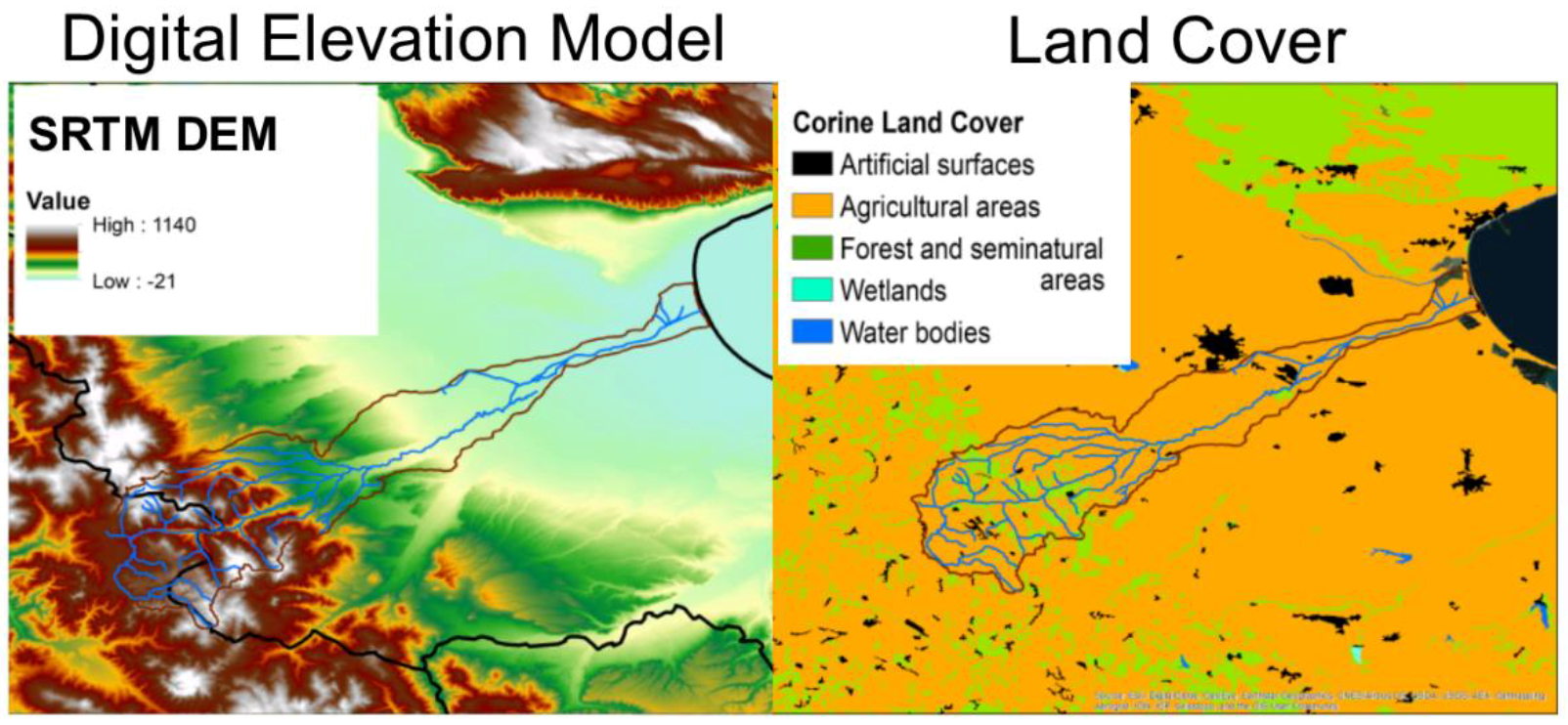
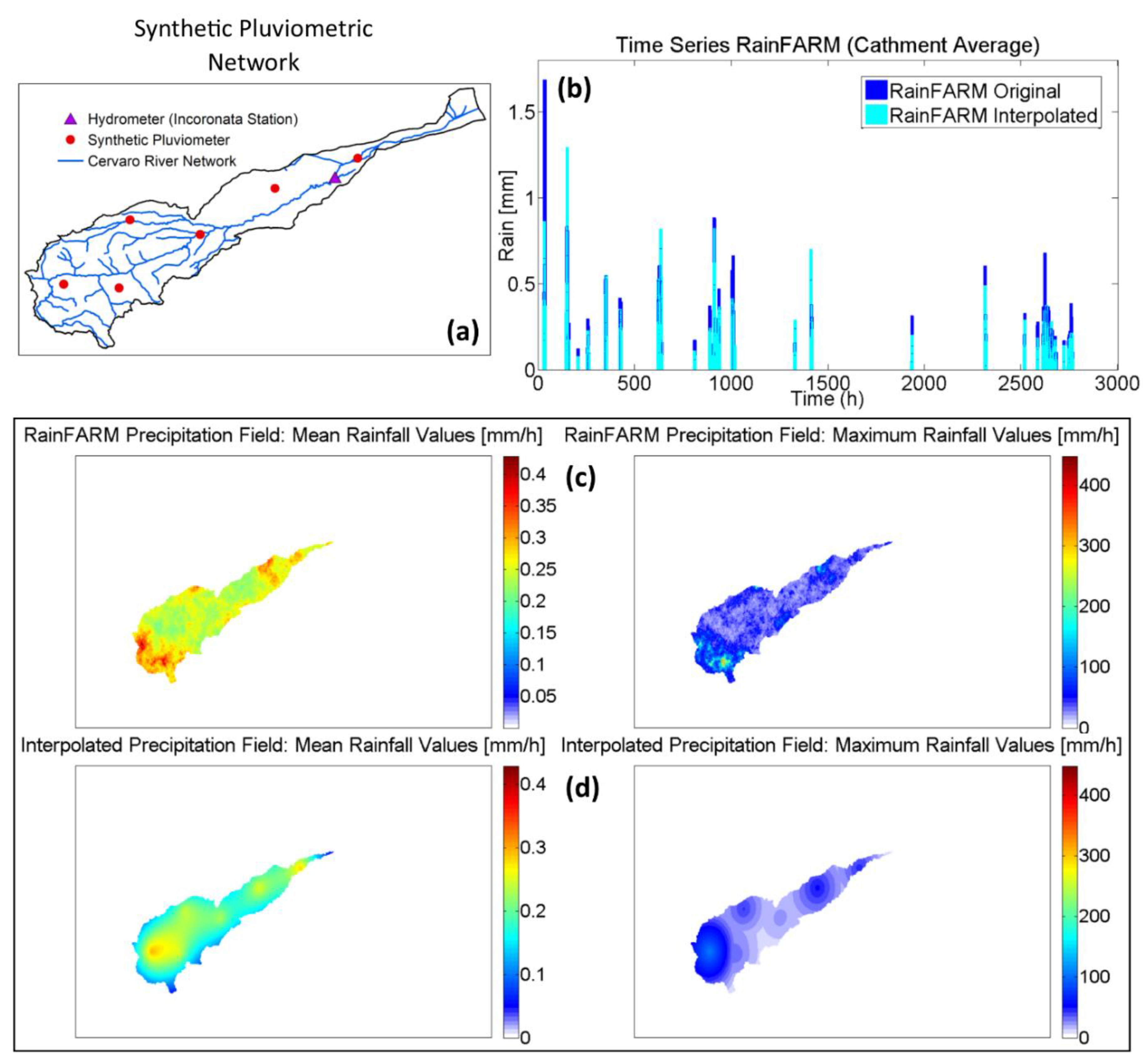
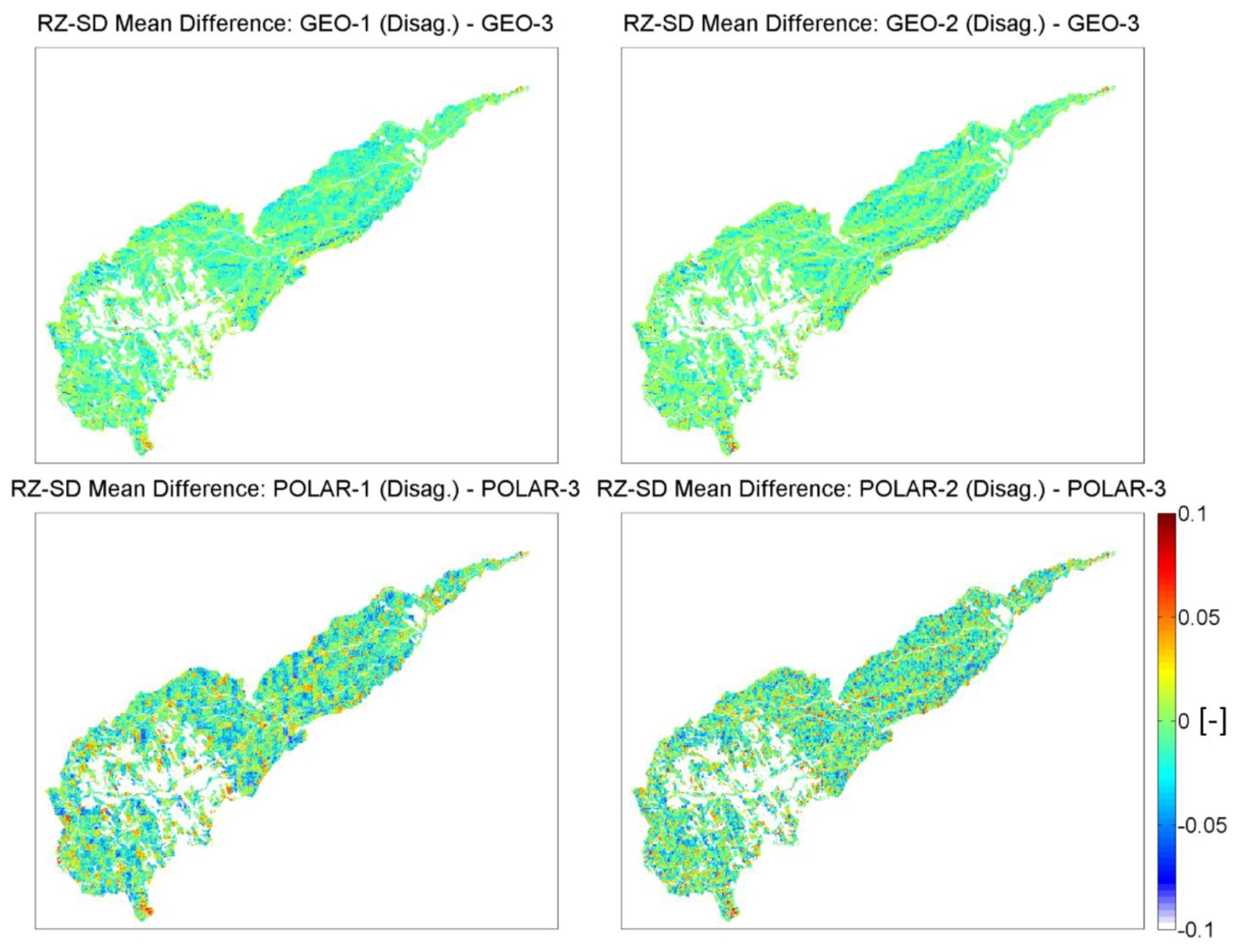
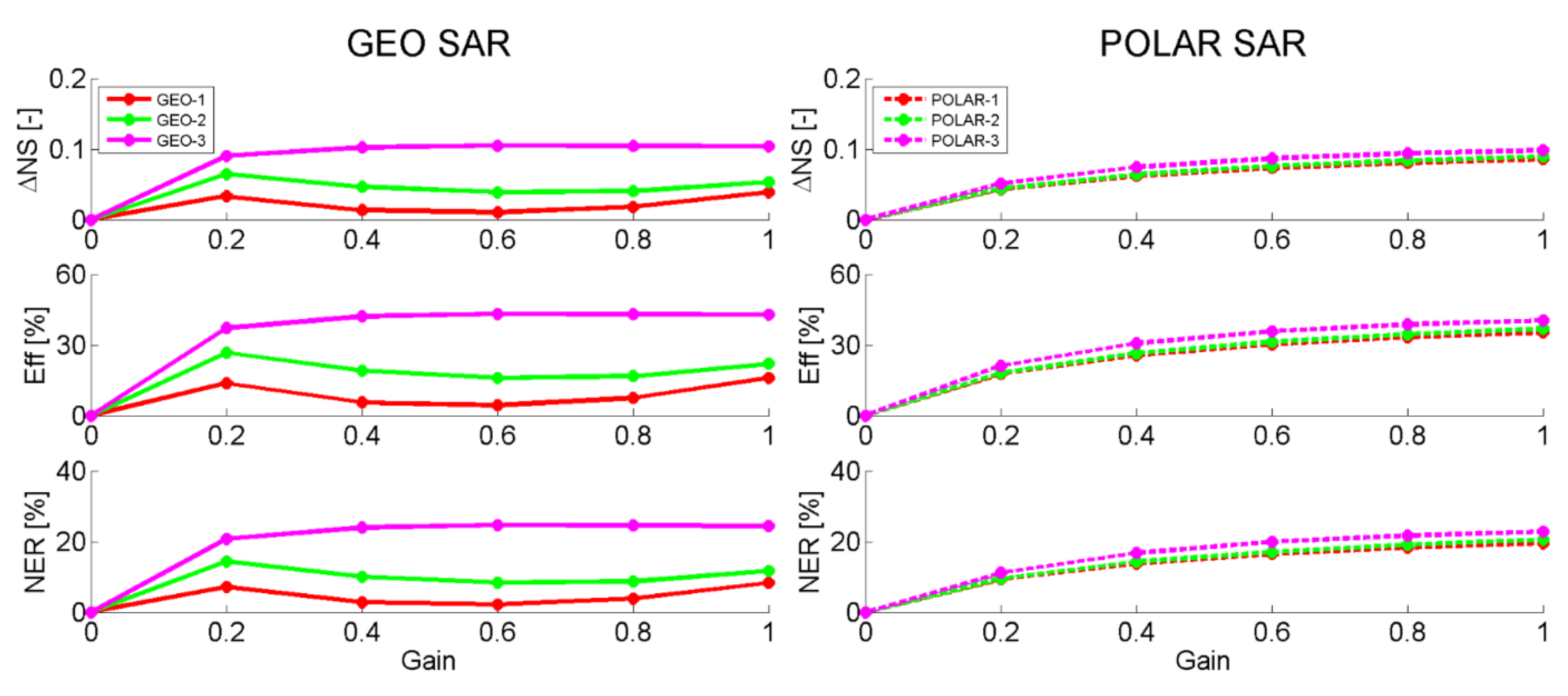
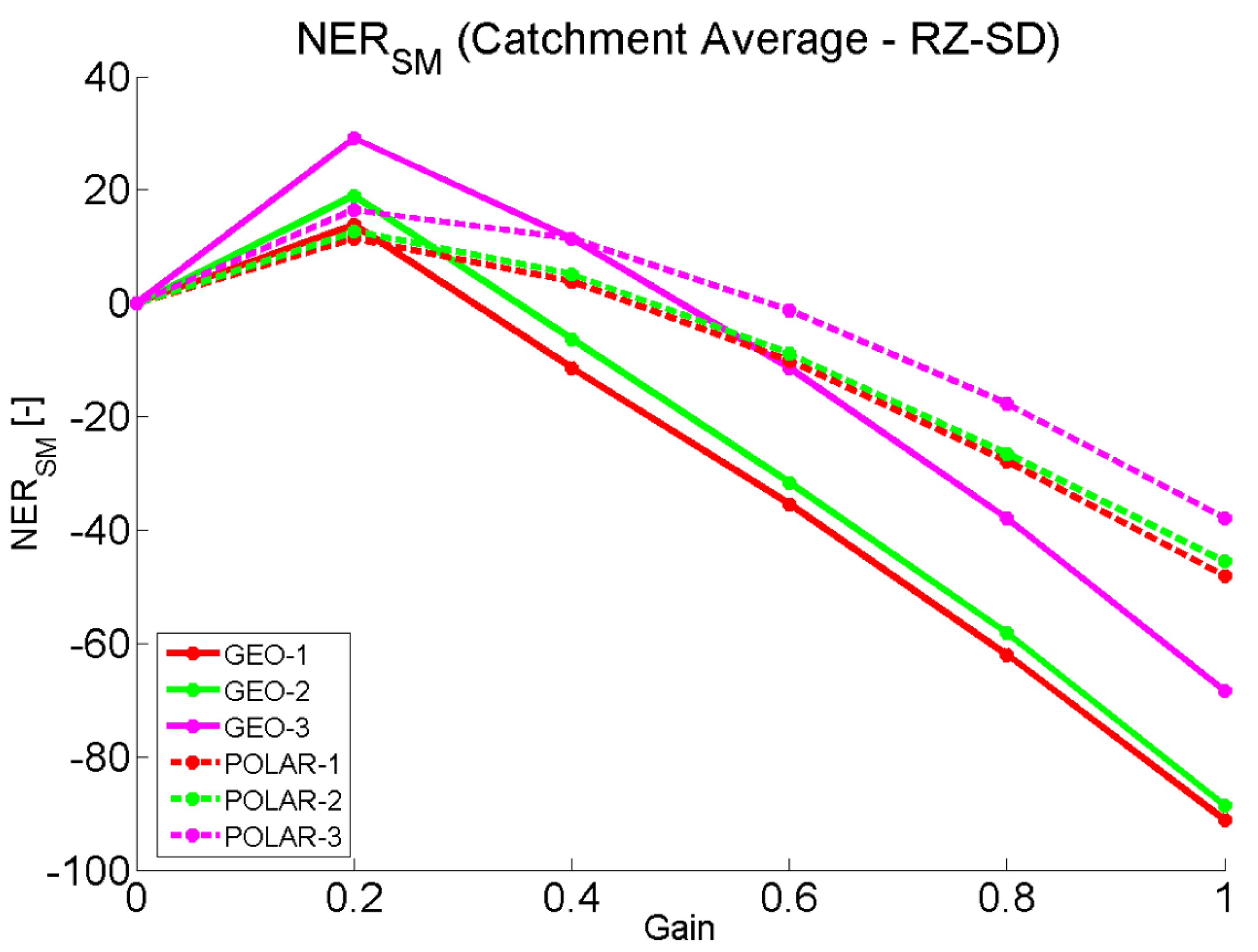
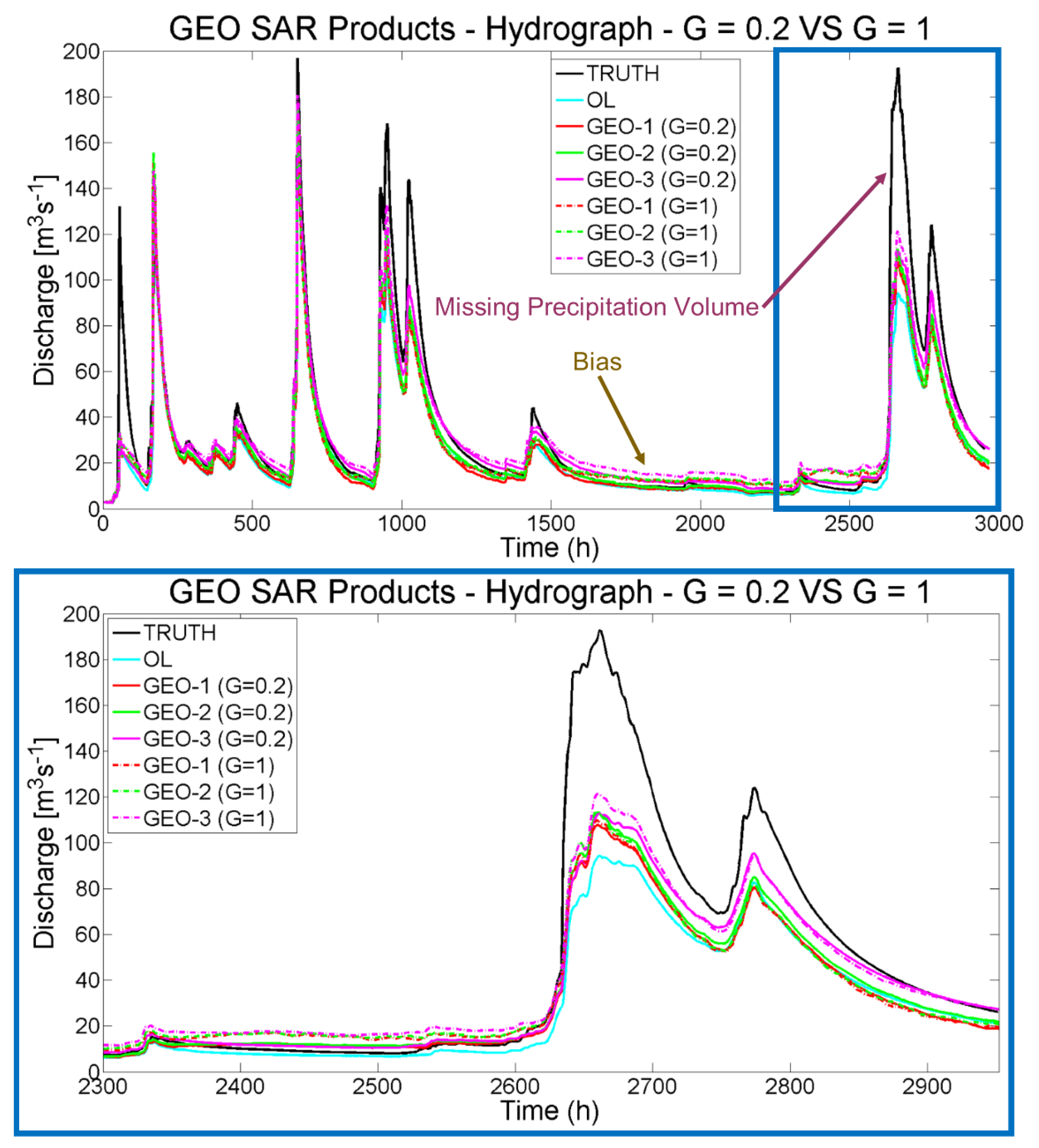
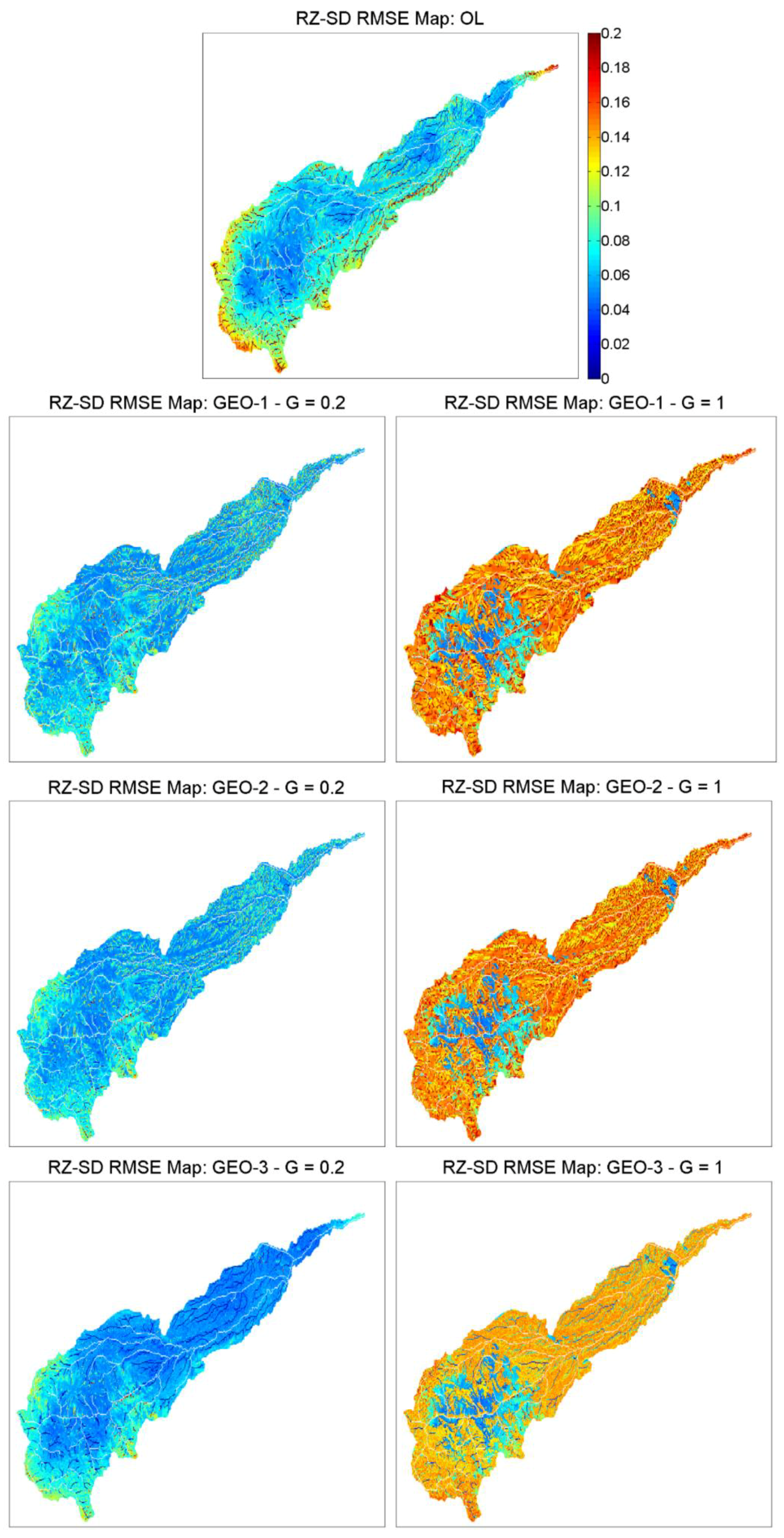
Table 1.
GEO SAR product specifications considered in the SM-DA exercises, and total number of GEO SAR-like observations that were assimilated in the whole model domain. The total number of the hourly time steps (i.e., TRUTH SM Maps) that composed the TRUTH and all the PERTURBED runs (including the OL) is 2952 (which corresponds to the number of hours in the time period ranging from 1 October 2016 00:00 to 31 January 2017 23:00).
| GEO SAR PRODUCT | SpR | TeR | Number of Observations |
|---|---|---|---|
| GEO-1 | 800 m | 1 h | 1968 |
| GEO-2 | 400 m | 2 h (average value) | 984 |
| GEO-3 | 100 m | 8 h (average value) | 246 |
Table 2.
S1 data considered to simulate the POLAR SAR SM assimilation. The total number of S1 images that were acquired over the Cervaro River Catchment in the time period under investigation and used in the SM-AD exercise were 58.
Table 2.
S1 data considered to simulate the POLAR SAR SM assimilation. The total number of S1 images that were acquired over the Cervaro River Catchment in the time period under investigation and used in the SM-AD exercise were 58.
| Relative Orbit Number | Pass Direction | Acquisition Time |
|---|---|---|
| 124 | Descending | 05:03 |
| 44 | Ascending | 16:57 |
| 146 | Ascending | 16:49 |
Table 3.
POLAR SAR product specifications considered in the SM-DA exercises, and total number of POLAR SAR-like observations that were assimilated.
Table 3.
POLAR SAR product specifications considered in the SM-DA exercises, and total number of POLAR SAR-like observations that were assimilated.
| POLAR SAR PRODUCT | SpR | TeR | Number of Observations |
|---|---|---|---|
| POLAR-1 | 800 m | Same as S1 | 58 |
| POLAR-2 | 400 m | Same as S1 | 58 |
| POLAR-3 | 100 m | Same as S1 | 58 |
© 2018 by the authors. Licensee MDPI, Basel, Switzerland. This article is an open access article distributed under the terms and conditions of the Creative Commons Attribution (CC BY) license (http://creativecommons.org/licenses/by/4.0/).
Share and Cite
MDPI and ACS Style
Cenci, L.; Pulvirenti, L.; Boni, G.; Pierdicca, N. Defining a Trade-off Between Spatial and Temporal Resolution of a Geosynchronous SAR Mission for Soil Moisture Monitoring. Remote Sens. 2018, 10, 1950. https://doi.org/10.3390/rs10121950
AMA Style
Cenci L, Pulvirenti L, Boni G, Pierdicca N. Defining a Trade-off Between Spatial and Temporal Resolution of a Geosynchronous SAR Mission for Soil Moisture Monitoring. Remote Sensing. 2018; 10(12):1950. https://doi.org/10.3390/rs10121950
Chicago/Turabian StyleCenci, Luca, Luca Pulvirenti, Giorgio Boni, and Nazzareno Pierdicca. 2018. "Defining a Trade-off Between Spatial and Temporal Resolution of a Geosynchronous SAR Mission for Soil Moisture Monitoring" Remote Sensing 10, no. 12: 1950. https://doi.org/10.3390/rs10121950
Note that from the first issue of 2016, this journal uses article numbers instead of page numbers. See further details here.