Compressive Sensing for Ground Based Synthetic Aperture Radar


Department of Information Engineering, University of Florence, via Santa Marta, 3, 50139 Firenze, Italy
*
Author to whom correspondence should be addressed.
Remote Sens. 2018, 10(12), 1960; https://doi.org/10.3390/rs10121960
Submission received: 10 October 2018
/
Revised: 30 November 2018
/
Accepted: 2 December 2018
/
Published: 5 December 2018
(This article belongs to the Special Issue Advances in Real Aperture and Synthetic Aperture Ground-Based Interferometry)
Abstract
:Compressive sensing (CS) is a recent technique that promises to dramatically speed up the radar acquisition. Previous works have already tested CS for ground-based synthetic aperture radar (GBSAR) performing preliminary simulations or carrying out measurements in controlled environments. The aim of this article is a systematic study on the effective applicability of CS for GBSAR with data acquired in real scenarios: an urban environment (a seven-storey building), an open-pit mine, and a natural slope (a glacier in the Italian Alps). The authors tested the most popular sets of orthogonal functions (the so-called ‘basis’) and three different recovery methods (l1-minimization, l2-minimization, orthogonal pursuit matching). They found that Haar wavelets as orthogonal basis is a reasonable choice in most scenarios. Furthermore, they found that, for any tested basis and recovery method, the quality of images is very poor with less than 30% of data. They also found that the peak signal–noise ratio (PSNR) of the recovered images increases linearly of 2.4 dB for each 10% increase of data.
1. Introduction
Ground-based synthetic aperture radar (GBSAR) systems are popular remote sensing instruments for short-term [1] and long-term [2] monitoring of landslides, glaciers [3], and mines [4] as well as for detecting small displacements of bridges [5] and dams [6].
The working principle of GBSAR is based on dense spatial sampling (steps smaller than a quarter of wavelength) along the synthetic aperture (usually a linear mechanical guide).
Compressive sensing (CS) is a recent sampling paradigm [7,8] which asserts one can recover certain signals from far fewer samples or measurements than traditional methods use. Its basic idea relies on the ‘sparsity’ of the signals of interest (the radar signals typically have this property [9]), and the incoherence of the sensing modality. The latter property is obtained through random sampling.
Generally speaking, CS can be applied in frequency domain (for reducing the number of transmitted frequencies) or in spatial domain (for reducing the number of spatial steps along the synthetic aperture).
In 2010, Huang et al. [10] applied CS to step-frequency through-wall radar that scanned along a horizontal mechanical guide. In 2011, Karlina and Sato [11] proposed to apply CS to GBSAR and they performed simulations, as well as Zonno in 2014 [12]. Yigit [13] extended CS to GB-SAR/ISAR acquisition modality and performed measurements in controlled environment. The interferometric properties of CS-GBSAR have been demonstrated by Giordano el al. [14] in 2015.
At the state of the art, CS techniques appear very promising for GBSAR applications, but all the cited works are relative to radar acquisitions in controlled environments (anechoic chamber or short-range experiments with controlled targets). Therefore, the crucial question is if these techniques are effectively applicable with data acquired in real scenarios, like GBSAR images of large buildings, landslides, open-pit mines, and glaciers.
Furthermore, a few specific questions about the CS methods have to be addressed. The first one is how to choose the orthogonal set of functions (the basis) that are used for recovering the signal. The possible bases are countless. The possible recovery algorithms are many as well. Therefore, a general selection criterion is necessary both for basis selection and recovery method. Another question is: what is an acceptable compression with real data. The claims declared in works that use simulated data or acquisitions performed in very cooperative scenarios are probably too optimistic.
Finally, we noticed that in previous papers [12,14] the ϕ matrix (see next chapter for his definition) is built by under-sampling the complete set of data acquired along a single scan. It means that each line could use a different set of positions along the scan. In this article, the ϕ matrix is built using the same reduced set of data for all the lines. This could reduce the incoherence of sampling (and so the quality of reconstruction), but it is a solution that could be easily implemented with a physical array or with a MIMO (multiple input multiple output), such as in [15,16,17].
2. Materials and Methods
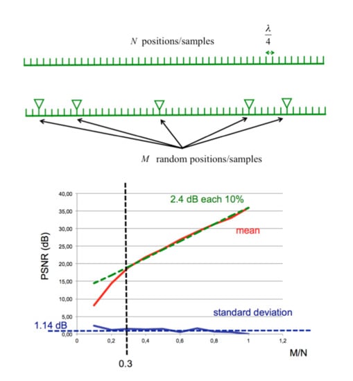
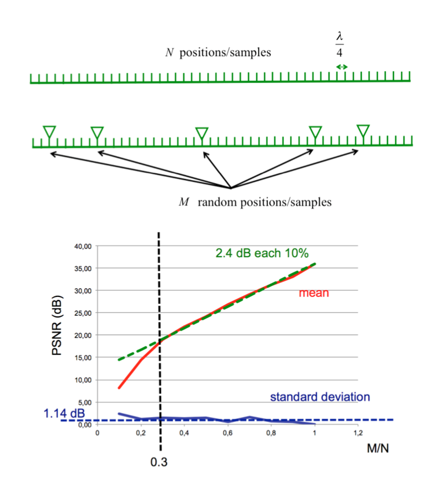
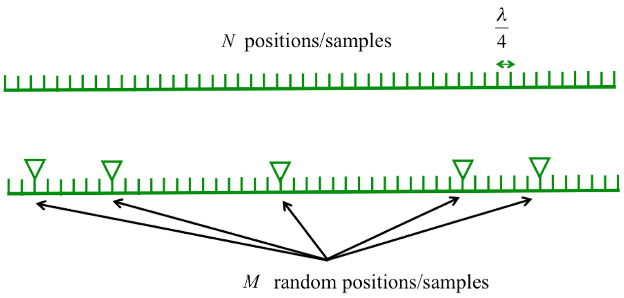
Compressive sensing theory states a sparse signal can be recovered by fewer samples than what is required by the Nyquist theorem. With reference to Figure 1, a standard GBSAR transmits and receives at N positions along a linear mechanical guide. The Nyquist theorem requires that the spatial step has to be smaller than a quarter of wavelength (λ/4) for omnidirectional antennas (this constraint is a bit more relaxed for directional antennas, but it is not essential in the discussion that follows). Let E be the vector of the N samples acquired according the Nyquist theorem. A subset of M random positions is selected between the N positions. These M positions are the effective points where the radar-head performs the measurements that will be used for recovering the complete set of N samples.
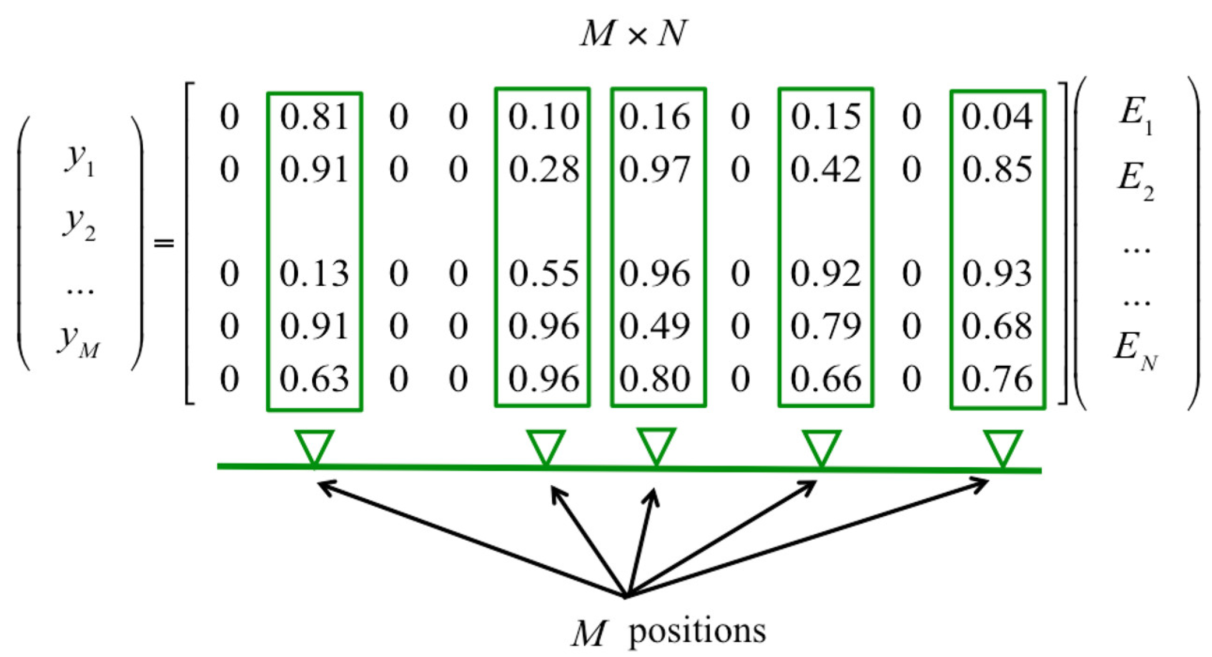
The next step is to define M variables (ym) as random linear combinations of the N samples using only the M positions as sketched in Figure 2.
The vector y of the M variables can be written as
with ϕ matrix M × N as defined in Figure 2. It should be noted that the vector y is a measurable quantity, as it can be calculated from the NA measurements.
A radar signal is often sparse in a suitable set of functions. As an example, an ideal scenario with a single point-target in far field appears as a single peak in the domain of spatial frequencies. Inspired by this idea, we can write the vector E as
where
and where b is the vector of the coefficients of spatial Fast Fourier Transform (FFT) of the signal. If the signal is sparse, many coefficient bn are almost null.
The FFT or the DCT (discrete cosine transform) should be able to effectively represent ideal point targets, but they could be a too rough approximation for more realistic distributed targets. Wavelets transforms give better results with distributed targets [18]. The possible complete sets of wavelets are countless, so we have limited this study to the most popular sets [18,19,20,21] specifically: Haar wavelets, Daubechies wavelets, biorthogonal wavelet, coiflets, symlets, LeGall wavelets, and discrete Meyer wavelets.
By substituting Equaiton (2), in Equaiton (1), the vector y can be expressed as
with θ = ϕΨ. This matrix is the so-called ‘dictionary’. Equaiton (4) is a linear system with many more variables than equations. It is an ill-posed problem, but it can be solved with a suitable recovery method. The most popular are: l1-minimization [22], l2-minimization [23], and orthogonal matching pursuit [24]. Using one of these methods, the vector b is recovered, so the E vector of N samples is obtained by Equation (2).
The procedure described above has to be repeated for each frequency for obtaining the matrix Ek,i, with k-index ranging from 1 to Nf (number of frequencies) and i-index ranging from 1 to N.
The next step is to focus the matrix Ek,i using a back-propagation algorithm that takes into account of the phase history of each contribution relative to one specific position and one frequency.
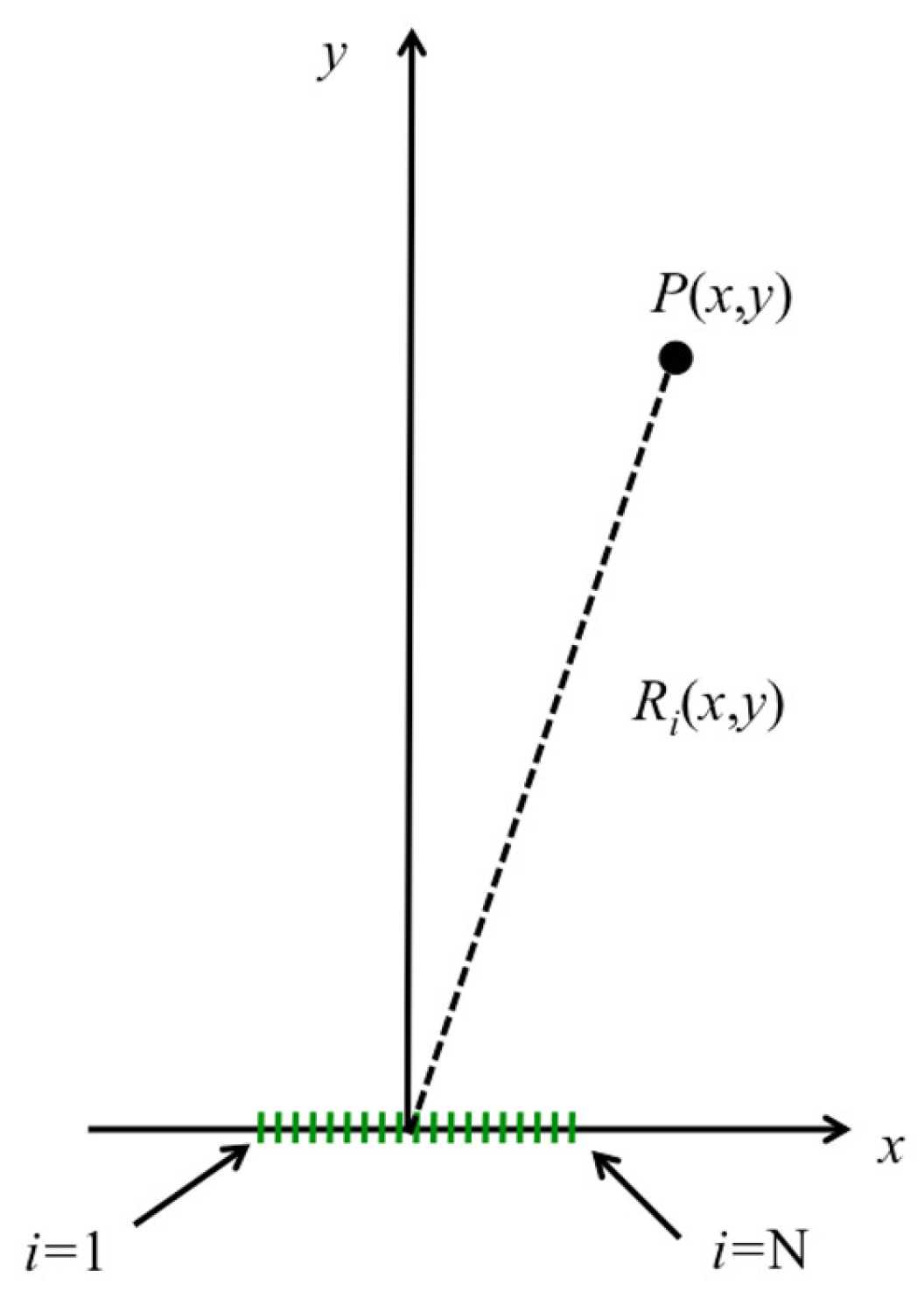
With reference to Figure 3, the image value I(x,y) in a generic image point P(x,y) can be calculated as
where c is the speed of light. This formula is correct but computationally very inefficient. More efficient algorithms make use of FFT and interpolation (see for example: [25]).
Since I(x,y) is a complex number, it provides the phase information too. This can be exploited for generating differential interferograms. Displacement maps can be obtained from differential interferograms using the well-known relationship [5]
where Δr(x,y) is the displacement in the point P(x,y), Δϕ(x,y) is the differential phase in the point P(x,y), and λ is the wavelength at the central frequency.
3. Results
3.1. Simulations
The CS algorithms have been preliminary tested with the simulation of a single target at 150 m distance in front of radar. The used parameters were: initial frequency f1 = 9.915 GHz, final frequency f2 = 10.075 GHz, number of frequencies Nf = 801, length of the mechanical scan L = 1 m, number of samples (according to Nyquist theorem) N = 100.
The quality of the recovered images were estimated with the peak signal–noise ratio (PSNR) calculated as
where Ri,j is the reference GBSAR image obtained from the data sampled according to Nyquist theorem without application of CS techniques; Ii,j is the image obtained using the CS techniques. Both images are complex matrix m × n. As rule of thumb, images with PSNR lower than 20–25 dB appear of low quality, with features hardly recognizable [26].
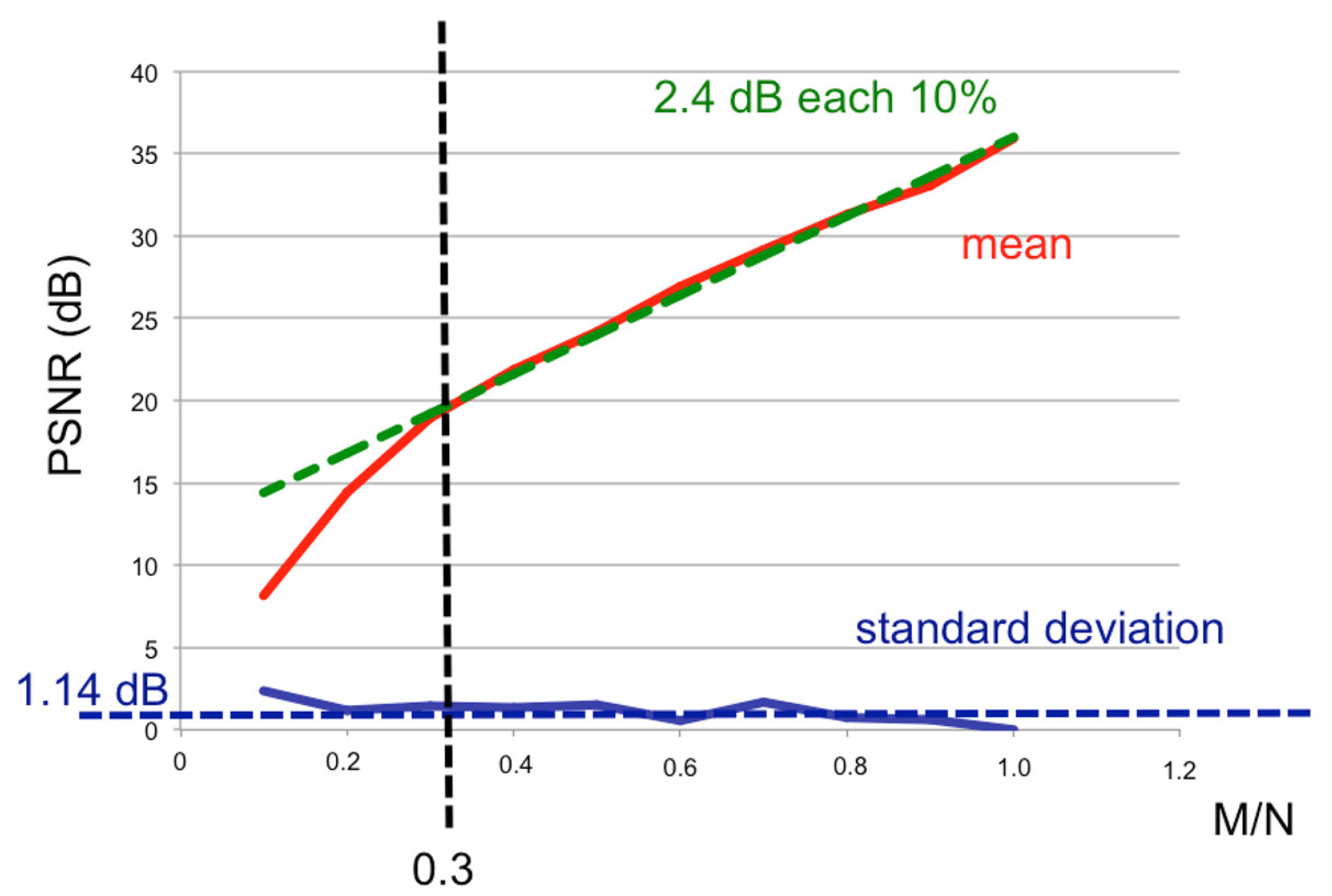
The used basis was the Haar wavelets, the recovery method was l2–minimization (this choice of Haar wavelets will be motivated in the experimental section, l2–minimization has been selected because it works even with a number of variable smaller than the number of equations, nevertheless the choice of both basis and recovery method is not essential for the discussion that follows). The PSNR has been calculated for an image 200 × 200 in polar coordinates. The range limits were 100 m and 200 m. The azimuth limits were −30 deg and +30 deg.
Figure 4 shows the plots of PSNR versus M/N. Each PSNR was calculated as the average of 25 random iterations and the standard deviation of each value is reported in the plot (blue line). It is interesting to note that for M/N > 0.3, PSNR increases linearly of 2.4 dB for each 10% increase of M/N. This is a notable result that we found also true for simulations of more complex scenarios (several targets), using different measurement parameters, different dictionaries, and different recovery methods, and in experimental data too. Note that PSNR does not tend to infinity for M = N, but it stops at about 37dB. The reason of it is related to the limited size of the φ matrix. As it is known, the CS reconstruction relies on the incoherence of both random sensing and the random coefficients of the matrix φ. When M = N, the sensing is no longer incoherent, but the incoherence of the ϕ coefficients persists and limits the quality of reconstruction. The φ coefficients are uniformly distributed random numbers between 0 and 1. When M = N, the number of elements is N × N = 100 × 100 = 10,000, the sum of 10,000 uniformly distributed random numbers between 0 and 1 gives exactly 37.0 dB, that is just the maximum PSNR obtained in Figure 4.
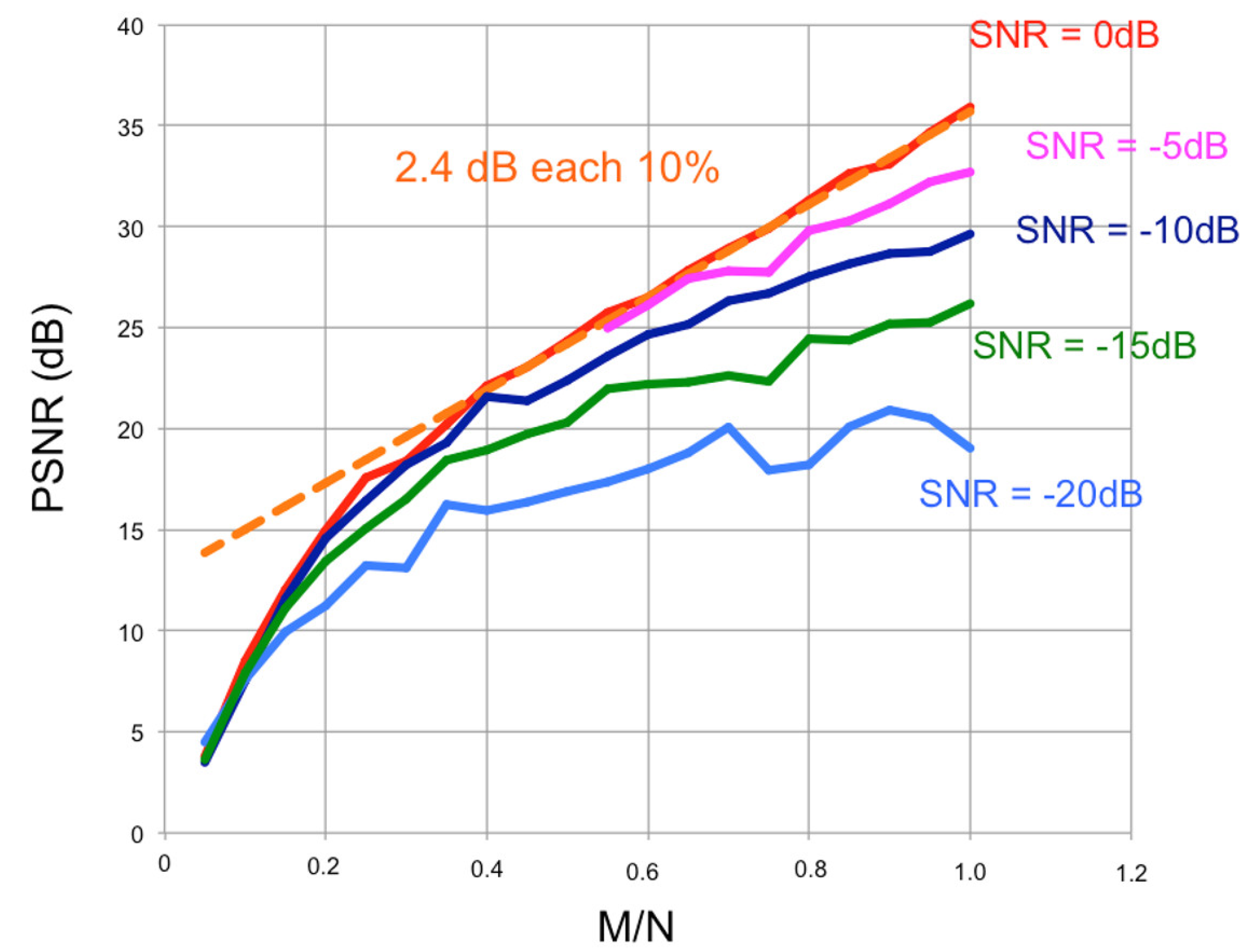
The noise can affect both PSNR and displacement retrieved by interferometry. In order to verify/evaluate it, we have repeated the simulations reported above with controlled Gaussian noise. Figure 5 shows the PSNR versus M/N calculated with different SNR values (the SNR reported in the plots is relative to one single measurement specified by one single frequency and one single position along the mechanical guide). Each PSNR value of the plots in Figure 6 is calculated as the average of 12 random iterations. As expected, by reducing the SNR the PSNR decreases. When the SNR of a single measurement is >0, the PSNR is practically equal to the PSNR without noise calculated in the previous chapter.
As mentioned above, the noise can give an error in the displacement retrieved by interferometry. In order to verify/evaluate it, we have estimated the phase error (Δϕ) and we have converted it in displacement error (ΔR) using the well-known relationship [5]:
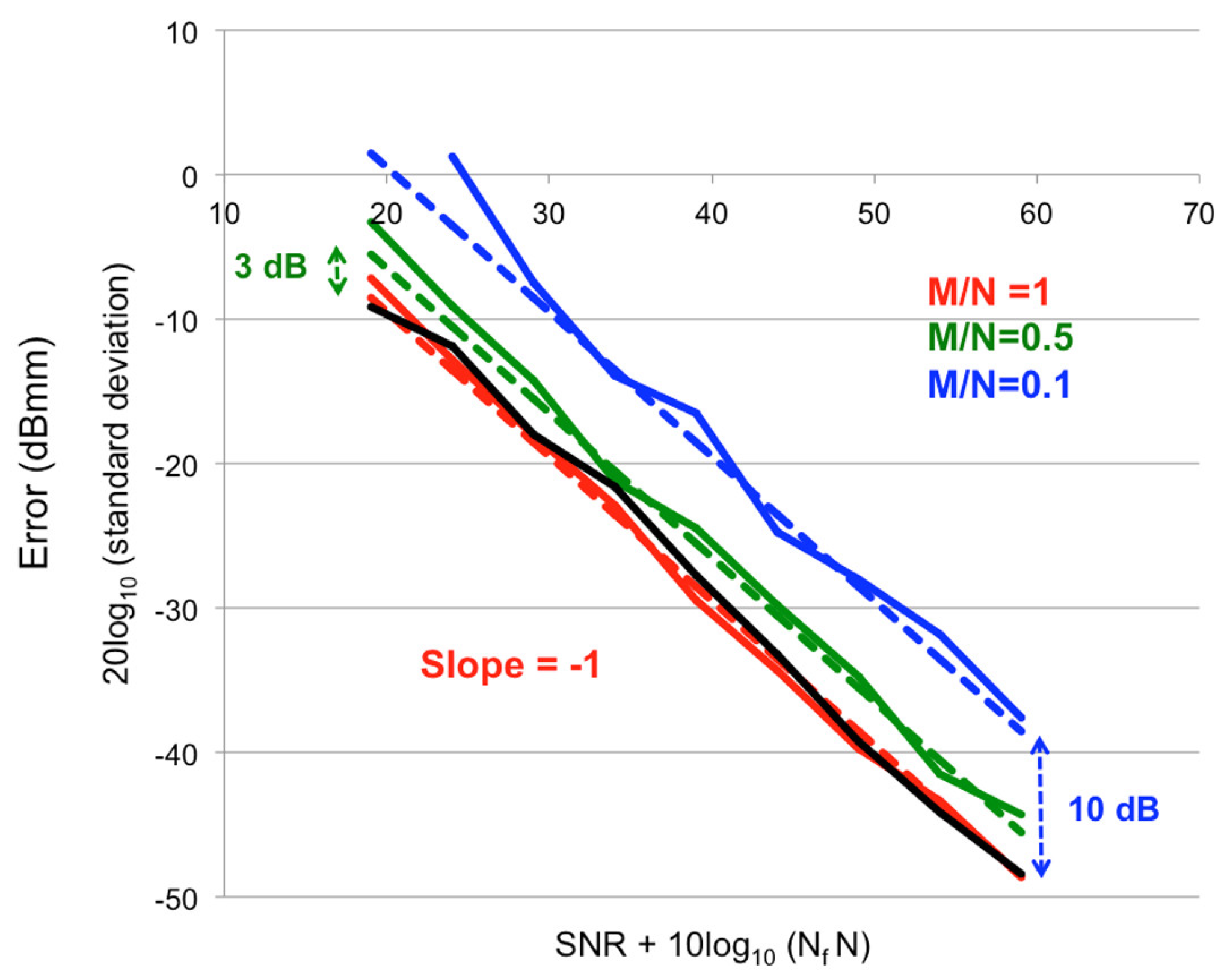
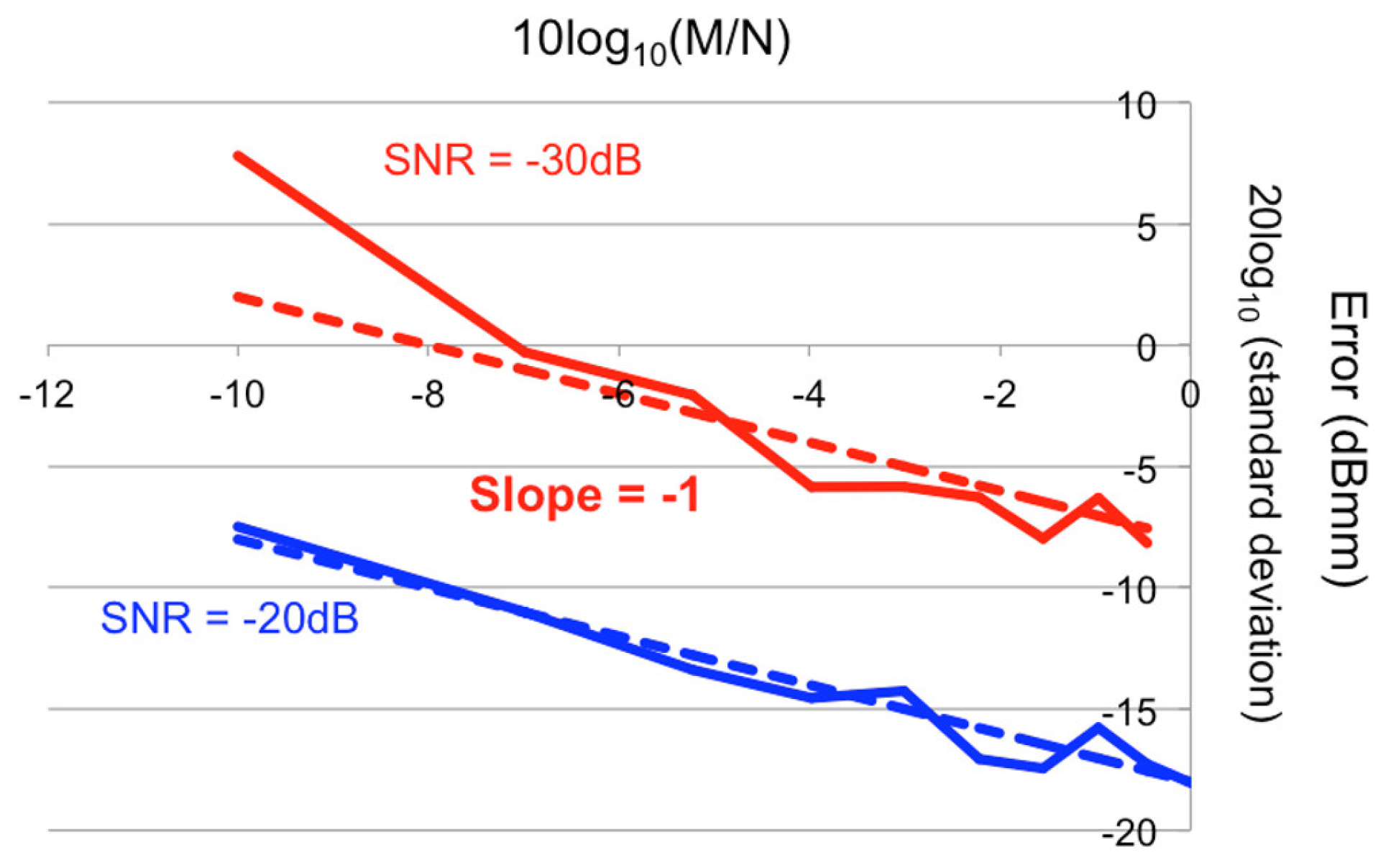
Figure 6 shows the estimated error in function of SNR. Each PSNR value is calculated as the average of 40 random iterations. For NA/N = 1 the error plot in function of SNR overlaps perfectly the plot of the error calculated without CS that, in log scale, is a straight line with slope −1. As expected, for M/N = 0.5 the error increases of 3dB and for M/N = 0.1 the error increases of 10 dB.
When M/N increases, the number of samples increases too. So the error should decrease. This intuitive idea has been verified with a simulation. Figure 7 shows how the error decreases increasing M/N, for two different values of the SNR. Both the plots are approximately straight lines with slope −1.
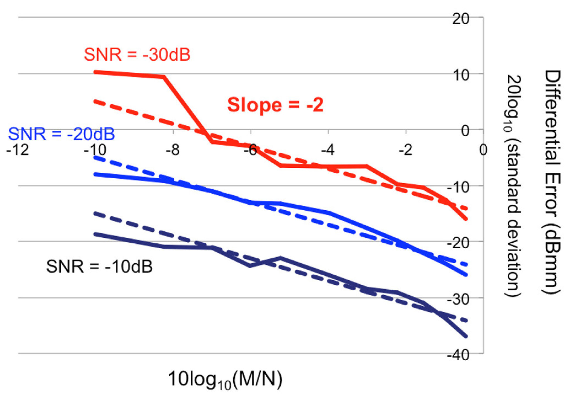
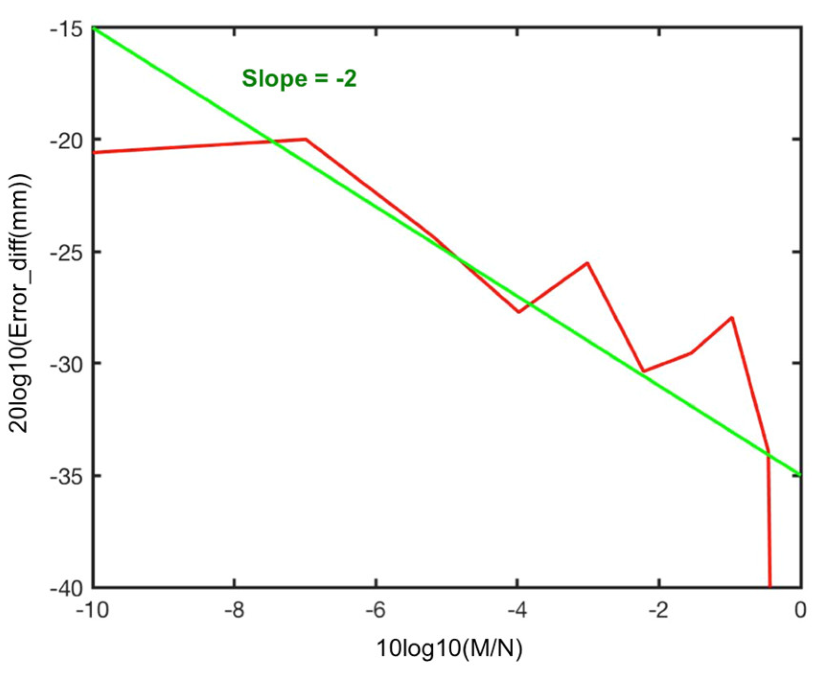
Generally speaking, the interferometric error could not depend only on Gaussian noise (i.e., on thermal noise). In that case, calculating the error in function of M/N does not make much sense, as it could be hard to obtain a straight line. On the contrary, the differential error (i.e., the error with respect to the image obtained using the CS with 100% of the samples) is expected to have a linear behavior (in log scale). Figure 8 shows the differential displacement in function of M/N for three different SNR. It is evident that the plots can be approximated as straight lines with a slope of −2.
3.2. Experimental Test Site “Campus”
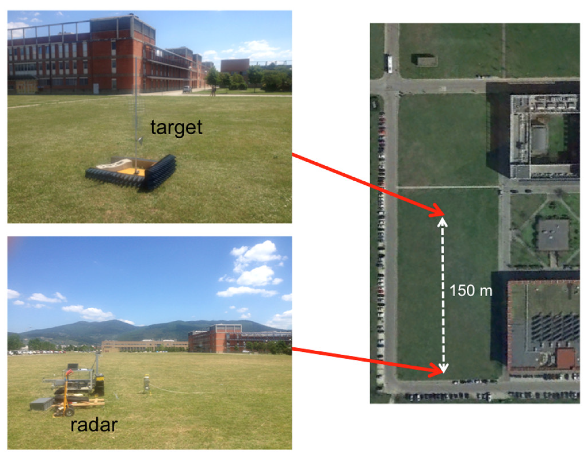
The CS techniques have been tested in a controlled experimental test site at the University of Florence (named “Campus”). A single metallic target, provided with a micrometric linear translator, has been positioned in front of the radar equipment at 150 m distance in a large flat garden, as shown in the pictures in Figure 9.
The measurement parameters were the same used in the simulations. The acquired experimental data have been used for testing the most popular bases and recovery methods. Specifically we used discrete cosine transform (dct), fast Fourier transform (fft), the Haar wavelts (haar), the Daubechies wavelets from order 2 to order 10 (db2–db10), seven biorthogonal wavelets (bior1.3, bior2.2, bior2.6, bior3.1, bior3.5, bior3.9, bior5.5), the “coiflets” from order 1 to 5 (coif1–coif5), the “simlets” from order 2 to 8 (sim2–sim8), LeGall wavelets (legal5.3), the discrete Meyer wavelets (dmey). As recovery methods, we used l1-minimization (L1), l2-minimization (L2), and orthogonal matching pursuit (OMP).
Table 1 reports the obtained PSNR for M/N = 0.5 and M/N = 0.33. The PSNR has been calculated for an image 200 × 200 in polar coordinates. The range limits were 100 m and 200 m. The azimuth limits were −30 deg and +30 deg.
In the table, we have highlighted the highest (in bold) and the lowest (in red bold) values. Using 50% of data, PSNR varies between 26.01 dB (Haar wavelets, OMP) and 21.89 dB (FFT, OMP). Using 30% of data, PSNR varies between 20.03 dB (Haar wavelets, OMP) and 15.87 dB (Bior3.1 wavelets, OMP).
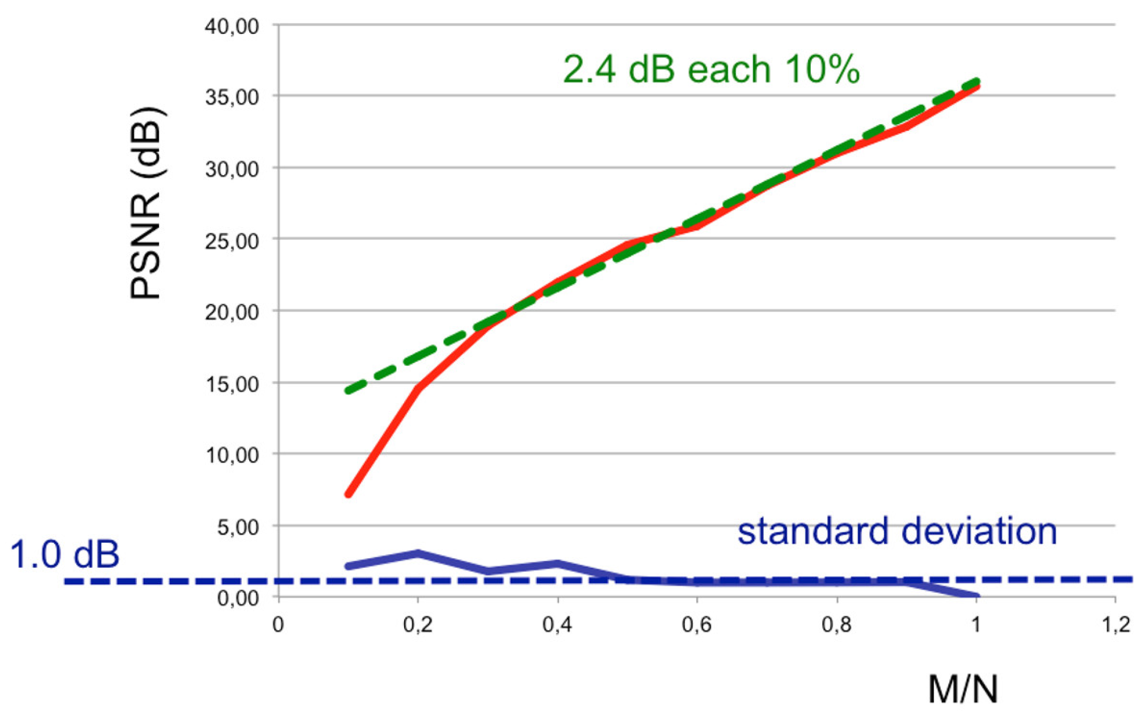
In simulated data, we have noted that PSNR increases linearly of 2.4 dB for each 10% increase of M/N. This relationship is perfectly confirmed also for these experimental data as shown in Figure 10.
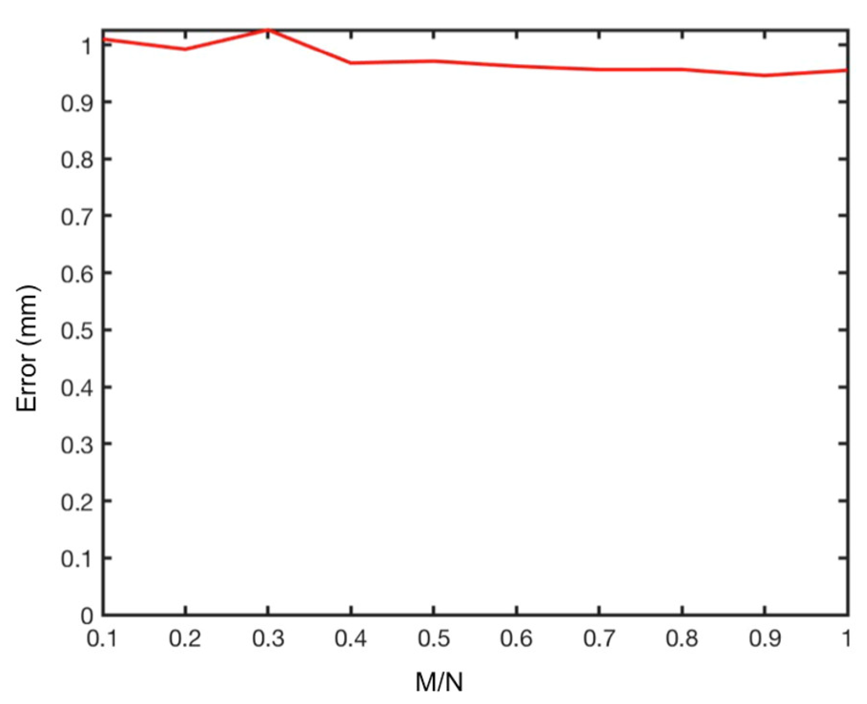
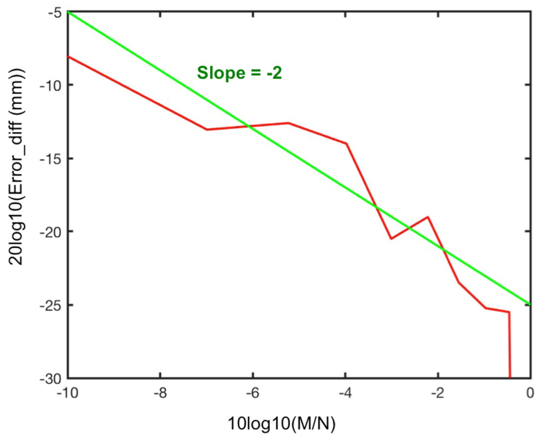
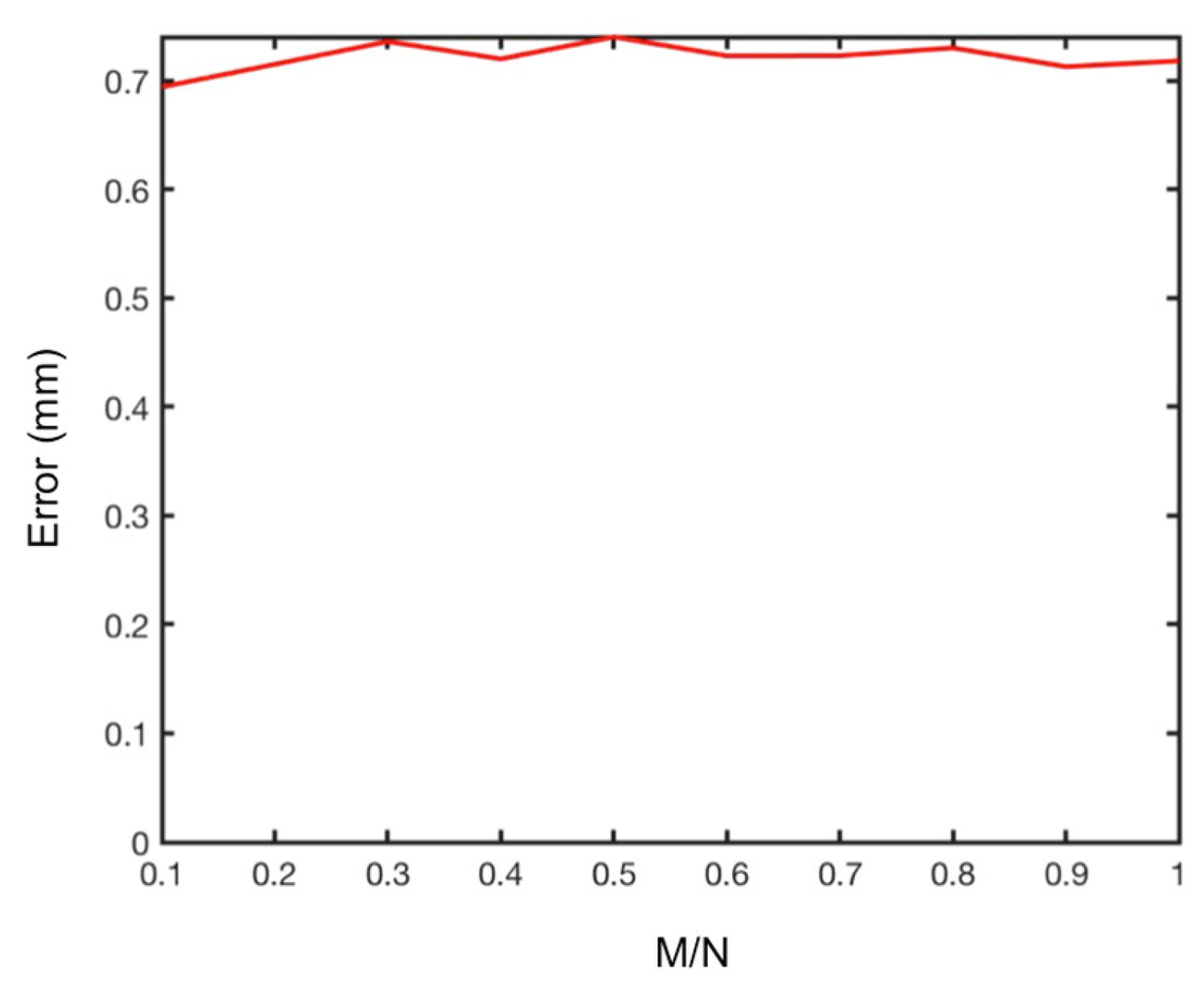
For evaluating the interferometric error we acquired 100 measurements in 96 h. By considering one pixel associated to a stable point of one building at about 200 m in the background, we evaluated the standard deviation of the displacement retrieved by interferometry. Figure 11 shows the obtained values varying M/N. The error is rather constant. It means that thermal (Gaussian) noise is not the main source of error. The effective contribution of thermal noise is more evident in the plot of the differential error (Figure 12) that confirms the error (in log scale) linearly decreases with slope −2, increasing the M/N (in log scale), as predicted by simulation.
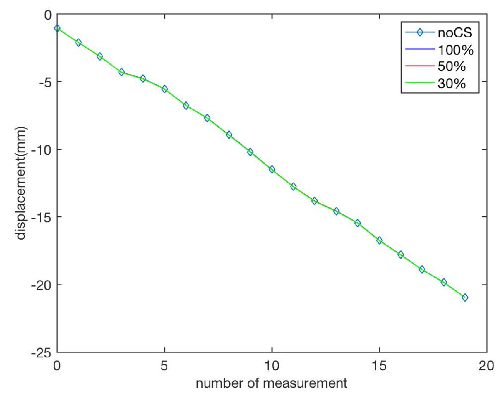
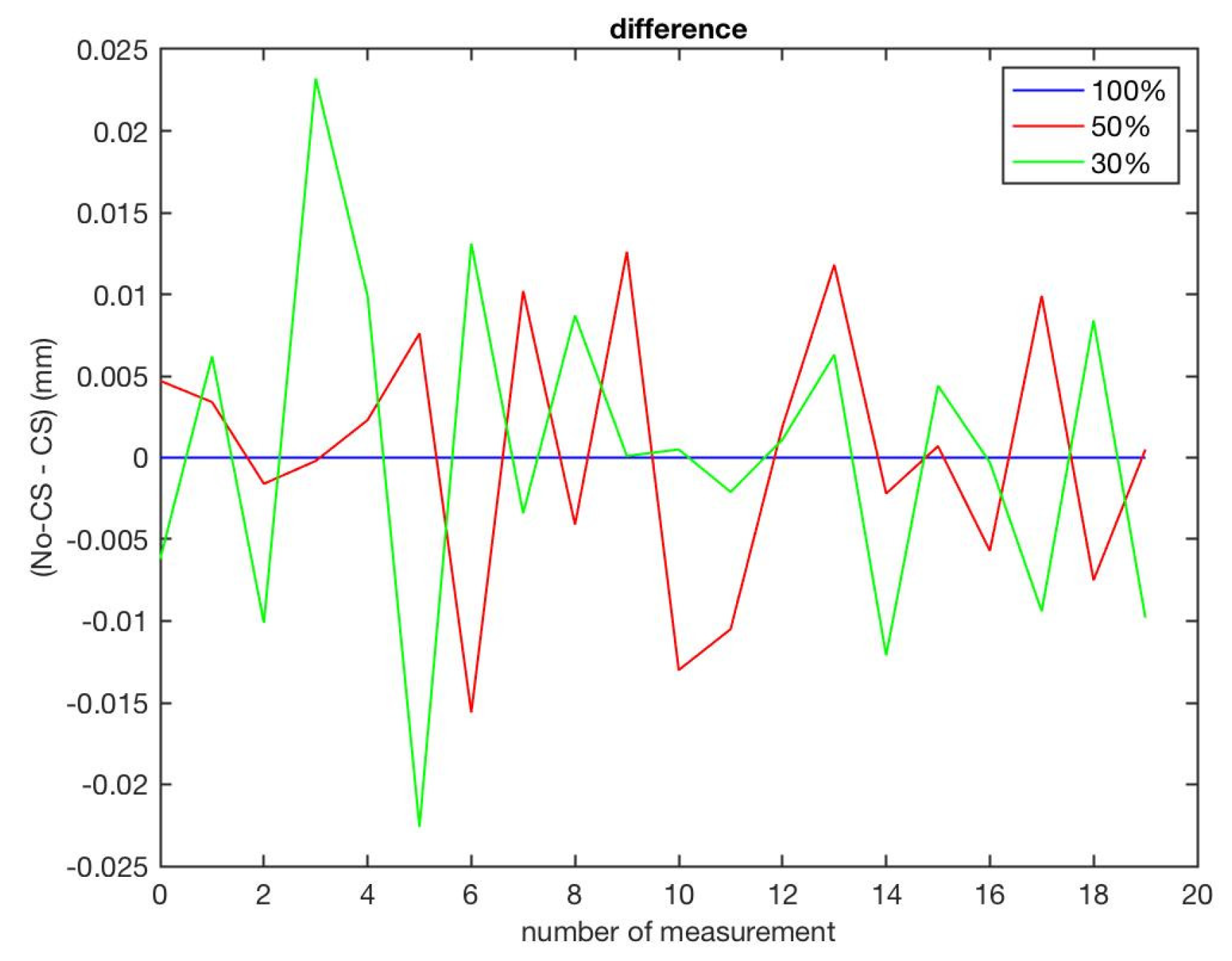
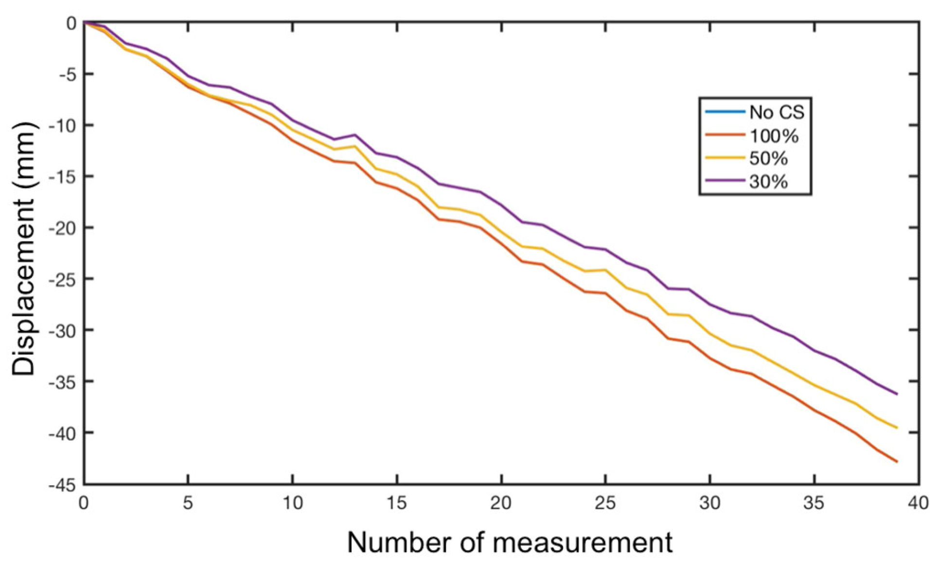
The metallic target in the middle of the grass was provided with a micrometric positioner able to translate it with a nominal accuracy of 0.1 mm. So, we performed 20 radar acquisitions by moving the target of 1 mm forward the radar after each acquisition. Figure 13 shows the cumulative displacement detected by interferometry using 100% of data without CS, using 100% of data with CS, using 50% of data with CS, and using 30% of data with CS. The four plots are practically overlapping. Figure 14 shows the plots of the differences. In the worst case (CS with 30% of data) the error is lower than 25 μm.
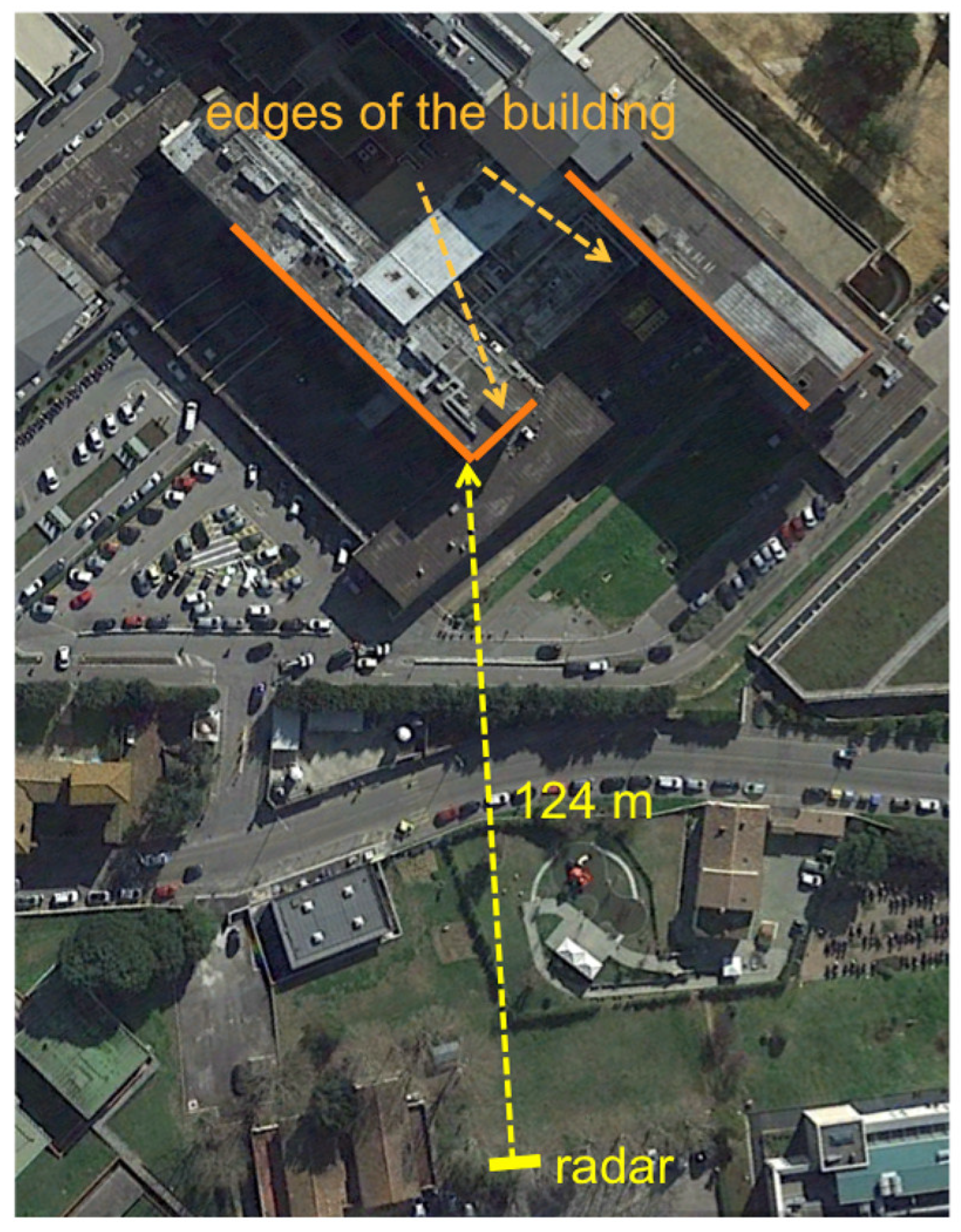
3.3. A Seven-Storey Building
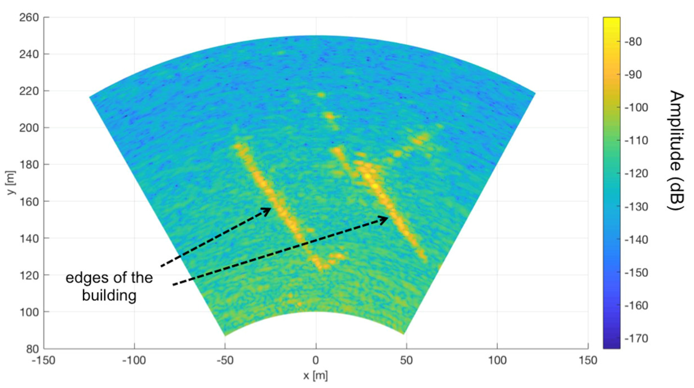
In order to test the application of CS techniques in an operative scenario representative of an urban environment, we performed radar measurements using as target the seven-storey building shown in Figure 15.
The measurement parameters were: initial frequency f1 = 9.915 GHz, final frequency f2 = 10.075 GHz, number of frequencies Nf = 801, length of the mechanical scan L = 1.8 m, number of samples (according to Nyquist theorem) N = 180. The obtained radar image (without application of CS techniques) is shown in Figure 16.
As well as for simulated data, and for the experimental data acquired at the “Campus” test site, we verified that PSNR increases linearly of 2.4 dB for each 10% increase of M/N and this relationship has been perfectly confirmed also for these experimental data (we do not report the graph for sake of brevity).
Table 2 reports the obtained PSNR for M/N = 0.5 and M/N = 0.3. We have highlighted the highest (in bold) and the lowest (in red bold) values. Using 50% of data, PSNR varies from 22.78 dB (db2 wavelets, OMP) to 8.19 dB (dct, OMP). Using 30% of data, the PSNR ranges between 19.12 dB (db5 wavelets or sym2 wavelets, OMP) and 1.80 dB (fft, OMP).
3.4. An Open-Pit Copper Mine
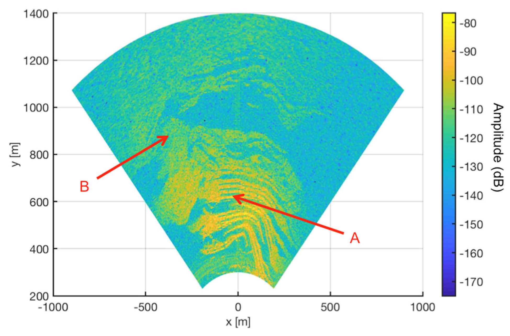
The most popular use of the GBSAR systems is the monitoring of open-pit mines. Therefore, we tested the application of the CS techniques to a representative case study of a copper mine in South America. The measurement parameters were: initial frequency f1 = 17.1 GHz, final frequency f2 = 17.3 GHz, number of frequencies Nf = 5333, length of the mechanical scan L = 1.275 m, number of samples (according to Nyquist theorem) N = 256. The obtained radar image (without application of CS techniques) is shown in Figure 17.
As well as for previous data, we verified that PSNR increases linearly of 2.4 dB for each 10% increase of M/N and this relationship has been perfectly confirmed also for these experimental data (we do not report the graph for sake of brevity).
Table 3 reports the obtained PSNR for M/N = 0.5 and M/N = 0.3. Using 50% of data, PSNR varies from 29.95 dB (Haar wavelets, OMP) to 17.25 dB (FFT, L2). Using 30%, the PSNR ranges between 29.44 dB (Haar wavelets, OMP) and 9.33 dB (FFT, OMP).
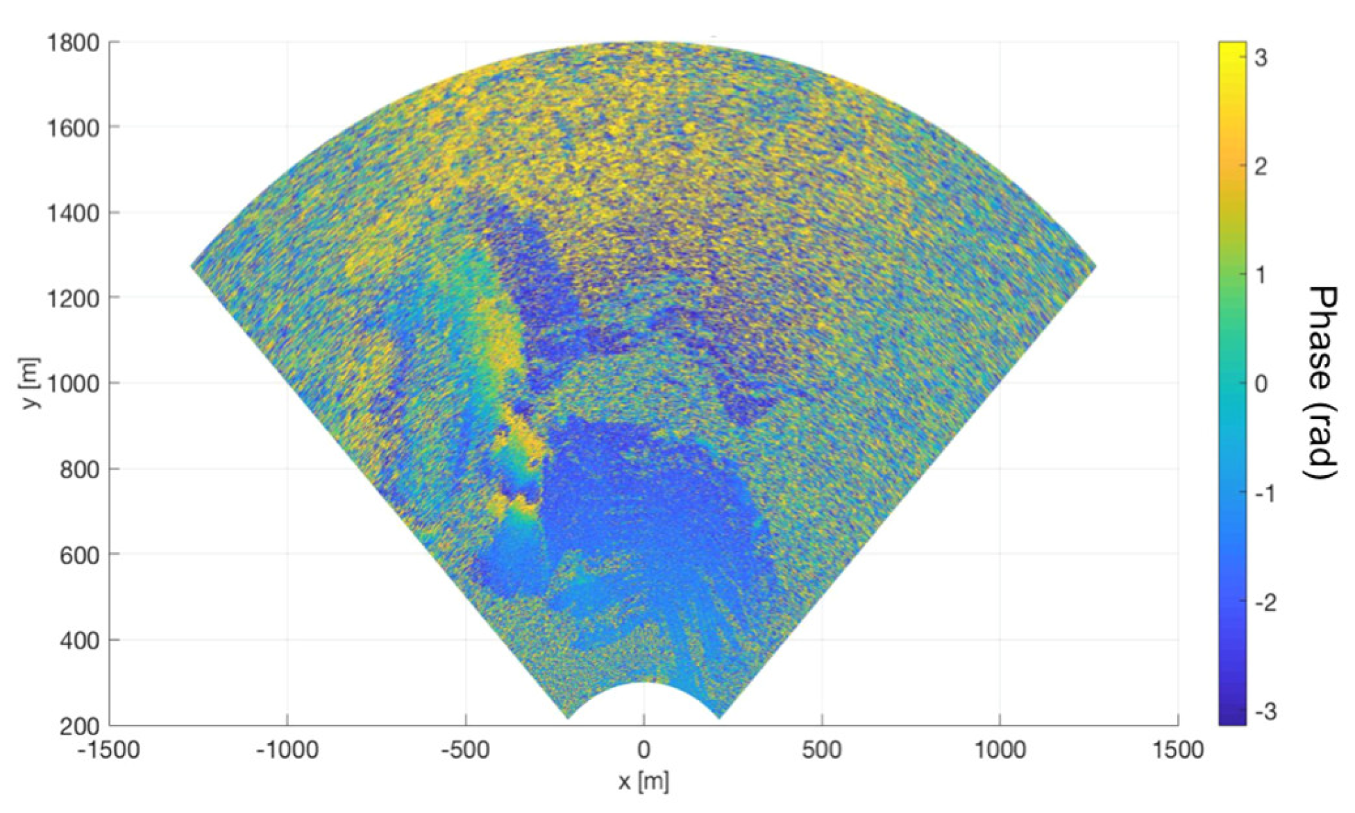
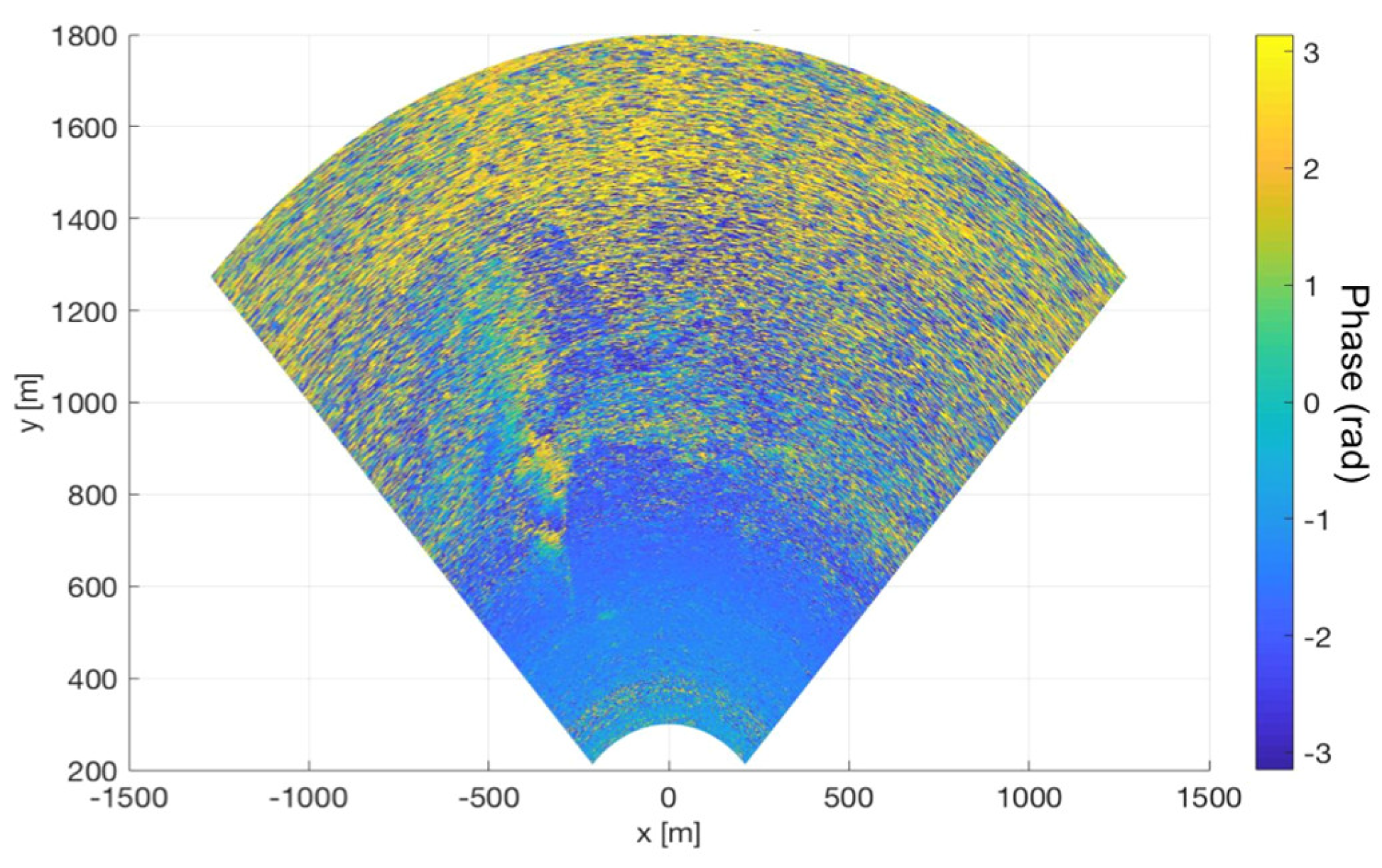
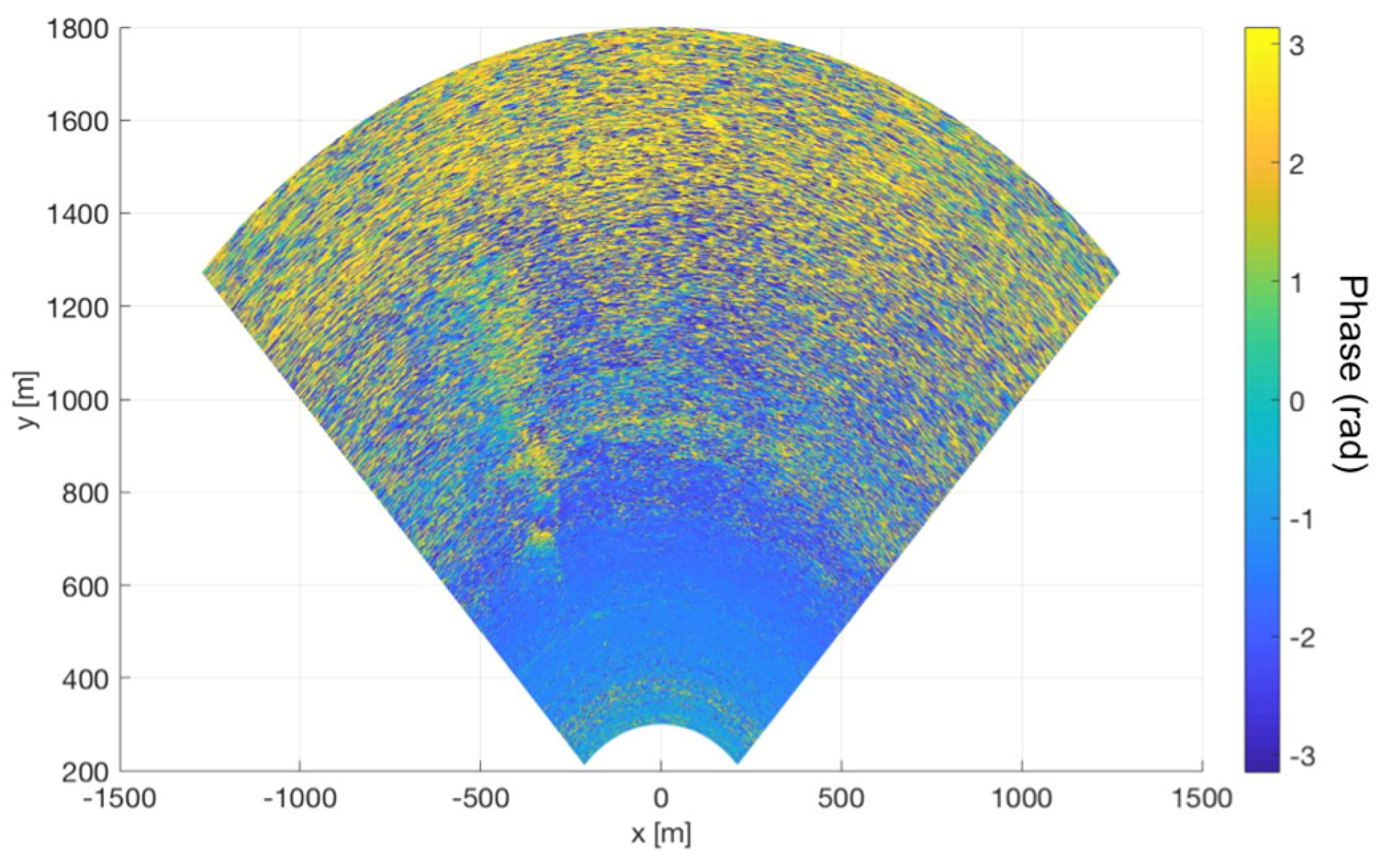
Figure 18 shows an interferogram between two images (focused without application of CS techniques) taken at different time. It shows a clear movement on the left side of the slope. In order to test the capability of the CS techniques to reconstruct interferograms, we applied them to 50% of data (Figure 19) and to 33% of data (Figure 20) using Haar wavelets and OMP.
In order to evaluate the interferometric error, we have processed 41 measurements acquired in 4 h and 20 min. By considering one pixel associated to one stable point (without visible fringes), we have evaluated the standard deviation of the displacement retrieved by interferometry. The point is labeled with letter A in Figure 17. Figure 21 shows the error (calculated as standard deviation) of the displacement at the stable point A varying M/N. The error is rather constant. It means that thermal (Gaussian) noise is not the main source of error. The effective contribution of thermal noise is more evident in the plot of the differential error (Figure 22). It confirms that the error linearly decreases (in log scale) with slope −2, increasing the M/N (in log scale), as predicted by simulation.
In order to verify the capability of CS to detect a cumulative displacement, we have taken into account the point B in Figure 18 where several fringes are evident in the interferograms (see Figure 19). Figure 23 shows the plot obtained without CS and the plot obtained with CS applied to 100% of data are perfectly overlapping. The CS plots with 50% and 30% of data tend to underestimate the displacement.
3.5. A Glacier
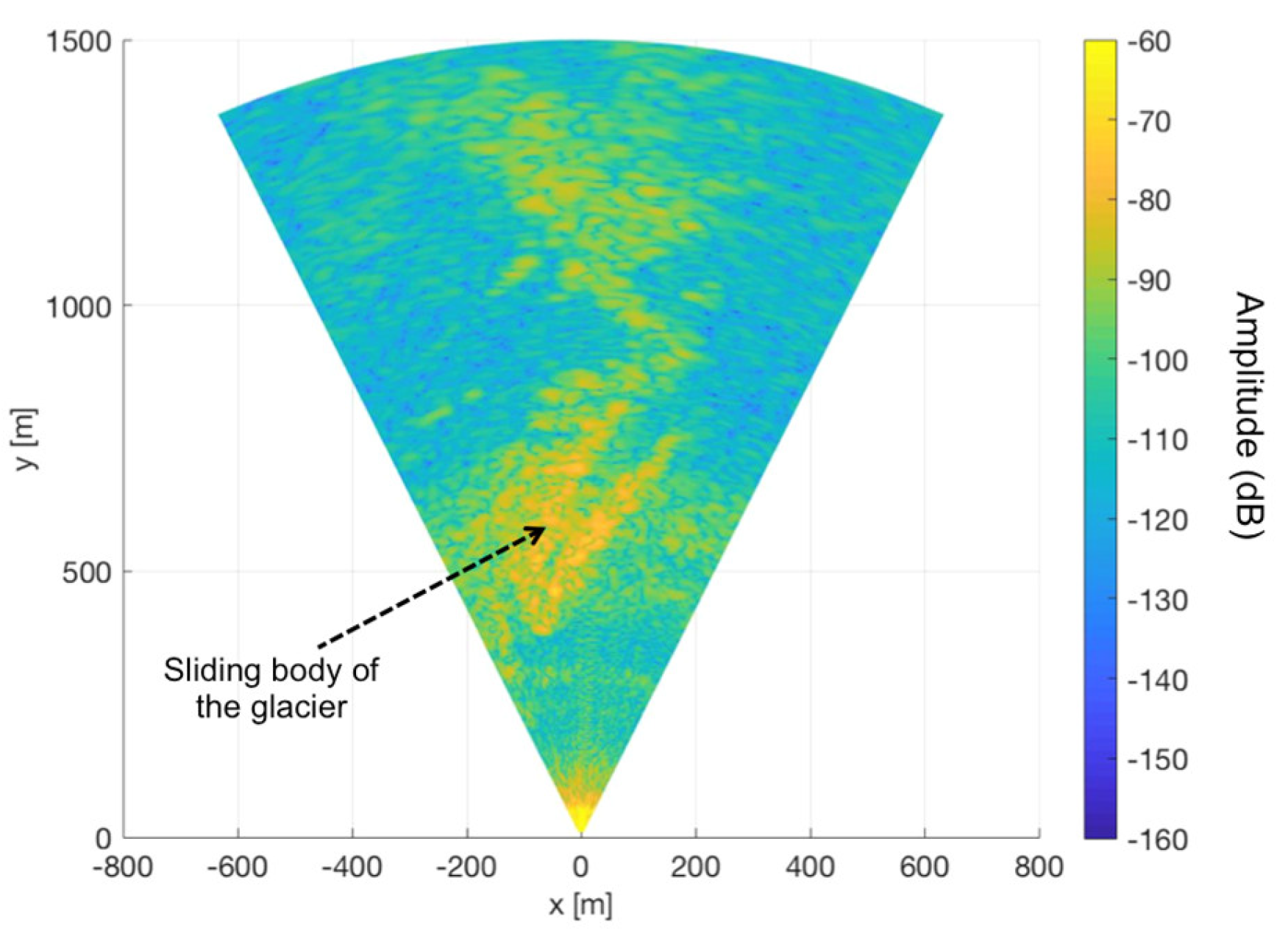
As test-site representative of a natural scenario we considered the “Belvedere” glacier in the Italian Alps. The data was acquired during a measurement campaign in 2006, whose details are reported in [3,27,28]. The measurement parameters were: f1 = 5.97 GHz, f2 = 5.99 GHz, Nf = 801, L = 1.71 m, N = 141. The obtained radar image (without application of CS techniques) is shown in Figure 24.
As well as for previous data, we verified that PSNR increases linearly of 2.4 dB for each 10% increase of M/N and this relationship has been perfectly confirmed also for these experimental data (we do not report the graph for sake of brevity).
Table 4 reports the obtained PSNR for M/N = 0.5 and M/N = 0.3. The PSNR has been calculated for an image 200 × 200 in polar coordinates. The range limits were 350 m and 1000 m. The azimuth limits were −25 deg and +25 deg. Using 50% of data, PSNR varies from 21.16 dB (Haar wavelets, OMP) to −3.50 dB (DCT, L2). Using 30%, the PSNR ranges between 16.52 dB (Haar wavelets, OMP) and −5.09 dB (FFT, L1).
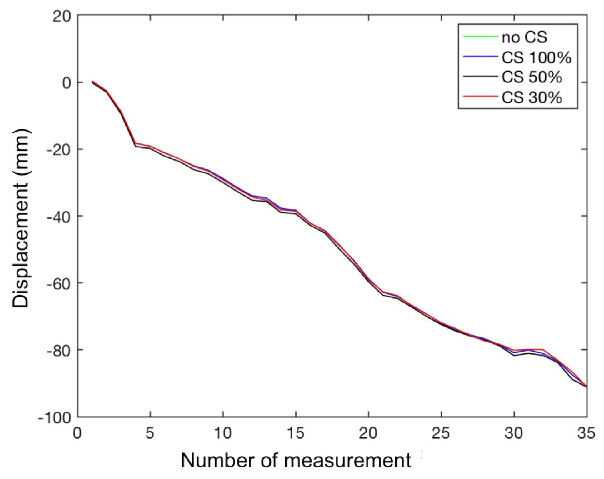
In order to verify the capability of CS to detect a cumulative displacement, we have taken into account a pixel inside the sliding body of the glacier. Figure 25 shows the plots obtained without CS and with CS applied to 100, 50, and 30% of data. The plots are almost perfectly overlapping.
Table 5 resumes the parameters of each measurement campaign and the highest value of PSNR obtained using 50% of data.
4. Conclusions
Authors found that CS techniques are able to reconstruct GBSAR images of good quality (PSNR > 20–30 dB) with almost 30–40% of data. Furthermore, they found that for more than 30% of data, the PSNR of the recovered image increases linearly of 2.4 dB for each 10% increase of data for all the tested bases and recovery methods. Nevertheless, the quality of reconstruction depends on the selected basis and recovery method. In a test site with just one single strong target, the best image has been obtained with FFT and OMP. In an urban scenario the best choice has been Daubechies wavelets and OMP. For an open-pit mine the highest quality image has been reconstructed with Haar wavelets and OMP. For a natural slope (a glacier) the optimal choice has been again Haar wavelets and OMP. In all cases, Haar wavelets with OMP gave good results (even if not always the best). Therefore, we can state that Haar wavelets with OMP is a reasonable choice for most practical cases. Furthermore, we found that CS reconstruction does not worsen significantly the interferometric error. The plots of the cumulative displacement recovered with 100, 50, and 30% of data overlaps almost completely the plot obtained without application of CS techniques. All these findings constitute the basic scientific starting point for designing optimal sparse array or multiple-input multiple-output (MIMO) radar able to exploit the CS techniques.
Author Contributions
M.P. conceived and designed the experiments; L.M. performed the experiments; N.R. analyzed the data; M.P. wrote the paper.
Funding
This research received no external funding.
Conflicts of Interest
The authors declare no conflicts of interest.
References
- Luzi, G.; Pieraccini, M.; Mecatti, D.; Noferini, L.; Macaluso, G.; Galgaro, A.; Atzeni, C. Advances in groundbased microwave interferometry for landslide survey: A case study. Int. J. Remote Sens. 2006, 27, 2331–2350. [Google Scholar] [CrossRef]
- Noferini, L.; Pieraccini, T.T.M.; Mecatti, D.; Macaluso, G.; Luzi, G.; Atzeni, C. Analysis of ground-based SAR data with diverse temporal baselines. IEEE Trans. Geosci. Remote Sens. 2008, 46, 1614–1623. [Google Scholar] [CrossRef]
- Noferini, L.; Mecatti, D.; Macaluso, G.; Pieraccini, M.; Atzeni, C. Monitoring of Belvedere Glacier using a wide angle GB-SAR interferometer. J. Appl. Geophys. 2009, 68, 289–293. [Google Scholar] [CrossRef]
- Liu, B.; Ge, D.; Li, M.; Zhang, L.; Wang, Y.; Zhang, X. Using GB-SAR technique to monitor displacement of open pit slope. In Proceedings of the International Geoscience and Remote Sensing Symposium (IGARSS), Beijing, China, 10–15 July 2016; pp. 5986–5989. [Google Scholar]
- Pieraccini, M.; Tarchi, D.; Rudolf, H.; Leva, D.; Luzi, G.; Bartoli, G.; Atzeni, C. Structural static testing by interferometric synthetic radar. NDT E Int. 2000, 33, 565–570. [Google Scholar] [CrossRef]
- Jenkins, W.; Rosenblad, B.; Gomez, F.; Le-garsky, J.; Loehr, E. Deformation measurements of earth dams using a ground based inter-ferometric radar. In Proceedings of the 2012 ASDSO Annual Conference on Dam Safety, Denver, CO, USA, 16–20 September 2012. [Google Scholar]
- Candès, E.J.; Wakin, M.B. An introduction to compressive sampling. IEEE Signal Process. Mag. 2008, 25, 21–30. [Google Scholar] [CrossRef]
- Massa, A.; Rocca, P.; Oliveri, G. Compressive sensing in electromagnetics-a review. IEEE Antennas Propag. Mag. 2015, 57, 224–238. [Google Scholar] [CrossRef]
- Hadi, M.A.; Alshebeili, S.; Jamil, K.; El-Samie, F.E.A. Compressive sensing applied to radar systems: An overview. Signal Image Video Process. 2015, 9, 25–39. [Google Scholar] [CrossRef]
- Huang, Q.; Qu, L.; Wu, B.; Fang, G. UWB through-wall imaging based on compressive sensing. IEEE Trans. Geosci. Remote Sens. 2010, 48, 1408–1415. [Google Scholar] [CrossRef]
- Karlina, R.; Sato, M. Compressive sensing applied to imaging by ground-based polarimetric SAR. In Proceedings of the 2011 IEEE International Geoscience and Remote Sensing Symposium (IGARSS 2011), Vancouver, BC, Canada, 24–29 July 2011. [Google Scholar]
- Zonno, M. GBSAR data focusing based on compressive sensing. In Proceedings of the 10th European Conference on Synthetic Aperture Radar EUSAR 2014, Berlin, Germany, 3–5 June 2014. [Google Scholar]
- Yiğit, E. Compressed sensing for millimeter-wave ground based SAR/ISAR imaging. J. Infrared Millim. Terahertz Waves 2014, 35, 932–948. [Google Scholar] [CrossRef]
- Giordano, R.; Guccione, P.; Cifarelli, G.; Mascolo, L.; Nico, G. Focusing SAR images by compressive sensing: Study of interferometric properties. In Proceedings of the International Geoscience and Remote Sensing Symposium (IGARSS), Milan, Italy, 26–31 July 2015; pp. 5352–5355. [Google Scholar]
- Feng, W.; Yi, L.; Sato, M. Near range radar imaging based on block sparsity and cross-correlation fusion algorithm. IEEE J. Sel. Top. Appl. Earth Obs. Remote Sens. 2018, 11, 2079–2089. [Google Scholar] [CrossRef]
- Tarchi, D.; Oliveri, F.; Sammartino, P.F. MIMO radar and ground-based SAR imaging systems: Equivalent approaches for remote sensing. IEEE Trans. Geosci. Remote Sens. 2013, 51, 425–435. [Google Scholar] [CrossRef]
- Hu, C.; Wang, J.; Tian, W.; Zeng, T.; Wang, R. Design and Imaging of Ground-Based Multiple-Input Multiple-Output Synthetic Aperture Radar (MIMO SAR) with Non-Collinear Arrays. Sensors 2017, 17, 598. [Google Scholar] [CrossRef] [PubMed]
- He, L.; Carin, L. Exploiting structure in wavelet-based Bayesian compressive sensing. IEEE Trans. Signal Process. 2009, 57, 3488–3497. [Google Scholar]
- Chui, C.K. An Introduction to Wavelets; Academic Press: San Diego, CA, USA, 1992. [Google Scholar]
- Walker, J.S. A Primer on Wavelets and Their Scientific Applications; CRC Press: Boca Raton, FL, USA, 1999. [Google Scholar]
- Wickerhauser, M.V. Adapted Wavelet Analysis from Theory to Software; IEEE Press: Piscataway, NJ, USA, 1994. [Google Scholar]
- Yang, A.Y.; Sastry, S.S.; Ganesh, A.; Ma, Y. Fast ℓ1-minimization algorithms and an application in robust face recognition: A review. In Proceedings of the 17th IEEE International Conference on Image Processing (ICIP), Hong Kong, China, 26–29 September 2010; pp. 1849–1852. [Google Scholar]
- Baraniuk, R.G. Compressive sensing [lecture notes]. IEEE Signal Process. Mag. 2007, 24, 118–121. [Google Scholar] [CrossRef]
- Tropp, J.A.; Gilbert, A.C. Signal recovery from random measurements via orthogonal matching pursuit. IEEE Trans. Inf. Theory 2007, 53, 4655–4666. [Google Scholar] [CrossRef]
- Pieraccini, M.; Miccinesi, L. ArcSAR: Theory, simulations, and experimental verification. IEEE Trans. Microw. Theory Tech. 2017, 65, 293–301. [Google Scholar] [CrossRef]
- Salomon, D. Data Compression: The Complete Reference; Springer: New York, NY, USA, 2004. [Google Scholar]
- Pieraccini, M.; Noferini, L.; Mecatti, D.; Macaluso, G.; Luzi, G.; Atzeni, C. Digital elevation models by a GBSAR interferometer for monitoring glaciers: The case study of Belvedere Glacier. In Proceedings of the IEEE International Geoscience and Remote Sensing Symposium, IGARSS 2008, Boston, MA, USA, 7–11 July 2008; Volume 4, p. IV-1061. [Google Scholar]
- Pieraccini, M.; Luzi, G.; Mecatti, D.; Noferini, L.; Atzeni, C. Ground-based SAR for short and long term monitoring of unstable slopes. In Proceedings of the 3rd European Radar Conference, EuRAD 2006, Manchester, UK, 13–15 September 2006; pp. 92–95. [Google Scholar]
Figure 1.
Sampling along the linear mechanical guide of a GBSAR.

Figure 2.
Definition of the M variables ym. The number different from zero in the matrix are selected randomly between 0 and 1.
Figure 2.
Definition of the M variables ym. The number different from zero in the matrix are selected randomly between 0 and 1.

Figure 3.
Focusing geometry.

Figure 4.
PSNR in function of M/N (simulated data).

Figure 5.
PSNR in function of M/N and SNR (simulated data).

Figure 6.
Displacement error in function of SNR for different M/N (simulated data). The dark line is the displacement error calculated without CS technique.
Figure 6.
Displacement error in function of SNR for different M/N (simulated data). The dark line is the displacement error calculated without CS technique.

Figure 7.
Displacement error in function of M/N for different SNR (simulated data).

Figure 8.
Differential displacement error in function of M/N for different SNR (simulated data).

Figure 9.
Experimental test site “Campus”.

Figure 10.
PSNR in function of M/N (data acquired at the experimental test site “Campus”).

Figure 11.
Displacement error in function of M/N for a stable point in the test site “Campus”.

Figure 12.
Differential displacement error in function of M/N for a stable point in the test site “Campus”.
Figure 12.
Differential displacement error in function of M/N for a stable point in the test site “Campus”.

Figure 13.
Cumulative measured displacement of the controlled metallic target at the test site “Campus”.
Figure 13.
Cumulative measured displacement of the controlled metallic target at the test site “Campus”.

Figure 14.
Differences between displacements detect through 100% CS, 50% CS, 30% and displacements detected using 100% of data without application of CS techniques (test site “Campus”).
Figure 14.
Differences between displacements detect through 100% CS, 50% CS, 30% and displacements detected using 100% of data without application of CS techniques (test site “Campus”).

Figure 15.
Aerial picture of the seven-storey building used as urban test site.

Figure 16.
Radar image (without application of CS techniques) of the building shown in Figure 15.
Figure 16.
Radar image (without application of CS techniques) of the building shown in Figure 15.

Figure 17.
Radar image (without application of CS techniques) of a copper mine in South America.

Figure 18.
Radar image (without application of CS techniques) of a copper mine in South America.

Figure 19.
Radar image obtained with 50% of data and CS.

Figure 20.
Radar image obtained with 33% of data and CS.

Figure 21.
Displacement error in function of M/N for a stable point in the open pit mine.

Figure 22.
Differential displacement error in function of M/N for a stable point in the open pit mine.
Figure 22.
Differential displacement error in function of M/N for a stable point in the open pit mine.

Figure 23.
Cumulative measured displacement of the point B in the open pit mine.

Figure 24.
Radar image (without application of CS techniques) of a glacier in the Italian Alps.

Figure 25.
Cumulative measured displacement of a pixel inside the sliding body the glacier.


Table 1.
PSNR calculated with different bases and recovery methods for experimental data acquired at the test site “Campus”.
Table 1.
PSNR calculated with different bases and recovery methods for experimental data acquired at the test site “Campus”.
| 50% | 33% | |||||
|---|---|---|---|---|---|---|
| L1 (dB) | L2 (dB) | OMP (dB) | L1 (dB) | L2 (dB) | OMP (dB) | |
| Dct | 22.92 | 22.89 | 22.29 | 18.77 | 19.02 | 19.62 |
| Fft | 22.61 | 22.73 | 21.89 | 17.00 | 17.16 | 17.45 |
| Haar | 24.83 | 24.83 | 26.01 | 18.30 | 18.30 | 20.03 |
| Db2 | 24.32 | 24.29 | 24.32 | 18.14 | 18.13 | 18.13 |
| Db3 | 24.32 | 24.33 | 24.36 | 17.68 | 17.66 | 18.01 |
| Db4 | 23.97 | 23.97 | 23.67 | 18.22 | 18.23 | 17.98 |
| Db5 | 23.71 | 23.73 | 23.10 | 17.49 | 17.48 | 17.35 |
| Db6 | 23.87 | 23.90 | 22.74 | 17.76 | 17.77 | 17.98 |
| Db7 | 23.24 | 23.25 | 22.60 | 17.41 | 17.45 | 16.11 |
| Db8 | 23.24 | 23.23 | 22.48 | 17.71 | 17.70 | 17.82 |
| Db9 | 23.26 | 23.27 | 21.46 | 17.71 | 17.72 | 17.82 |
| Db10 | 23.04 | 23.07 | 23.48 | 17.74 | 17.74 | 18.52 |
| Bior1.3 | 24.65 | 24.64 | 25.00 | 18.16 | 18.16 | 19.51 |
| Bior2.2 | 24.45 | 24.45 | 23.53 | 17.00 | 16.99 | 16.96 |
| Bior2.6 | 24.22 | 24.21 | 23.37 | 17.65 | 17.65 | 17.37 |
| Bior3.1 | 23.51 | 23.51 | 22.66 | 17.39 | 17.39 | 15.87 |
| Bior3.5 | 24.29 | 24.28 | 23.50 | 17.99 | 17.99 | 17.21 |
| Bior3.9 | 24.00 | 24.04 | 23.67 | 17.60 | 17.60 | 17.67 |
| Bior5.5 | 23.97 | 23.98 | 23.62 | 18.04 | 18.07 | 18.23 |
| Coif1 | 24.04 | 24.09 | 23.52 | 17.71 | 17.72 | 17.25 |
| Coif2 | 24.20 | 24.21 | 24.04 | 16.84 | 16.84 | 17.26 |
| Coif3 | 23.72 | 23.72 | 23.27 | 17.39 | 17.39 | 17.36 |
| Coif4 | 23.47 | 23.47 | 22.74 | 17.49 | 17.51 | 17.52 |
| Coif5 | 23.28 | 23.18 | 22.79 | 17.05 | 17.04 | 16.90 |
| Sym2 | 24.32 | 24.29 | 24.32 | 18.14 | 18.13 | 18.13 |
| Sym3 | 24.32 | 24.33 | 24.36 | 17.68 | 17.66 | 18.01 |
| Sym4 | 24.42 | 24.44 | 24.08 | 17.29 | 17.28 | 17.04 |
| Sym5 | 23.77 | 23.77 | 23.62 | 17.63 | 17.64 | 17.54 |
| Sym6 | 24.24 | 24.15 | 23.78 | 17.64 | 17.64 | 16.94 |
| Sym7 | 24.26 | 24.27 | 24.18 | 18.02 | 18.03 | 17.68 |
| Sym8 | 24.10 | 24.11 | 23.53 | 17.94 | 17.94 | 17.04 |
| Legall5.3 | 24.17 | 24.17 | 24.49 | 18.31 | 18.30 | 18.51 |
| Dmey | 23.60 | 23.60 | 23.56 | 17.93 | 17.94 | 17.96 |
Table 2.
PSNR calculated with different bases and recovery methods for experimental data acquired at the seven-storey building.
Table 2.
PSNR calculated with different bases and recovery methods for experimental data acquired at the seven-storey building.
| 50% | 33% | |||||
|---|---|---|---|---|---|---|
| L1 (dB) | L2 (dB) | OMP (dB) | L1 (dB) | L2 (dB) | OMP (dB) | |
| Dct | 16.47 | 16.59 | 8.16 | 11.04 | 10.85 | 5.93 |
| Fft | 15.62 | 15.30 | 10.72 | 9.33 | 9.98 | 1.80 |
| Haar | 22.73 | 22.73 | 21.59 | 19.00 | 19.00 | 18.42 |
| Db2 | 21.50 | 21.52 | 22.78 | 18.33 | 18.32 | 18.85 |
| Db3 | 21.60 | 21.62 | 22.72 | 18.13 | 18.13 | 18.86 |
| Db4 | 21.55 | 21.58 | 20.99 | 17.84 | 17.83 | 17.85 |
| Db5 | 21.01 | 21.02 | 21.60 | 17.91 | 17.93 | 19.12 |
| Db6 | 20.09 | 20.90 | 21.39 | 17.91 | 17.91 | 18.98 |
| Db7 | 20.48 | 20.52 | 20.67 | 17.79 | 17.75 | 18.49 |
| Db8 | 19.16 | 19.17 | 19.15 | 14.70 | 14.70 | 16.17 |
| Db9 | 19.11 | 19.14 | 17.81 | 17.05 | 17.04 | 16.32 |
| Db10 | 19.82 | 19.83 | 19.27 | 17.03 | 17.05 | 17.69 |
| Bior1.3 | 22.26 | 22.27 | 21.49 | 18.78 | 18.79 | 17.58 |
| Bior2.2 | 21.91 | 21.92 | 22.42 | 18.13 | 18.13 | 18.27 |
| Bior2.6 | 21.31 | 21.32 | 22.36 | 17.67 | 17.68 | 18.58 |
| Bior3.1 | 21.27 | 21.31 | 20.56 | 20.10 | 20.10 | 19.16 |
| Bior3.5 | 20.12 | 20.12 | 19.63 | 17.49 | 17.54 | 17.33 |
| Bior3.9 | 20.79 | 20.80 | 19.41 | 17.77 | 17.80 | 16.45 |
| Bior5.5 | 22.13 | 22.14 | 22.76 | 17.80 | 17.83 | 19.11 |
| Coif1 | 21.76 | 21.76 | 21.74 | 18.33 | 18.34 | 17.96 |
| Coif2 | 21.98 | 21.96 | 21.90 | 17.85 | 17.85 | 17.86 |
| Coif3 | 21.77 | 21.77 | 21.77 | 18.29 | 18.30 | 18.74 |
| Coif4 | 20.21 | 20.21 | 21.88 | 17.87 | 17.89 | 18.89 |
| Coif5 | 21.38 | 21.38 | 21.67 | 18.00 | 18.00 | 18.66 |
| Sym2 | 21.50 | 21.52 | 22.78 | 18.33 | 18.32 | 18.84 |
| Sym3 | 21.61 | 21.61 | 22.72 | 18.13 | 18.13 | 18.86 |
| Sym4 | 21.45 | 21.44 | 21.18 | 18.15 | 18.25 | 18.00 |
| Sym5 | 21.36 | 21.38 | 20.18 | 17.84 | 17.81 | 18.76 |
| Sym6 | 21.13 | 21.12 | 20.96 | 17.47 | 17.44 | 18.04 |
| Sym7 | 21.79 | 21.80 | 21.52 | 17.22 | 17.22 | 18.34 |
| Sym8 | 21.47 | 21.47 | 20.04 | 16.90 | 16.93 | 17.86 |
| Legall5.3 | 22.03 | 22.04 | 22.64 | 18.06 | 18.06 | 18.47 |
| Dmey | 20.55 | 20.59 | 19.16 | 17.46 | 17.46 | 16.95 |
Table 3.
PSNR calculated with different bases and recovery methods for experimental data acquired at a copper mine in South America.
Table 3.
PSNR calculated with different bases and recovery methods for experimental data acquired at a copper mine in South America.
| 50% | 33% | |||||
|---|---|---|---|---|---|---|
| L1 (dB) | L2 (dB) | OMP (dB) | L1 (dB) | L2 (dB) | OMP (dB) | |
| Dct | 17.54 | 18.23 | 17.36 | 15.84 | 16.31 | 15.90 |
| Fft | 17.41 | 17.25 | 15.26 | 11.69 | 12.44 | 10.05 |
| Haar | 29.39 | 29.39 | 29.95 | 25.81 | 25.81 | 29.44 |
| Db2 | 28.29 | 28.30 | 28.25 | 26.29 | 26.30 | 27.69 |
| Db3 | 25.34 | 25.37 | 27.85 | 23.94 | 23.94 | 26.22 |
| Db4 | 24.54 | 24.53 | 23.14 | 22.48 | 22.48 | 22.94 |
| Db5 | 25.69 | 25.70 | 23.68 | 21.38 | 21.37 | 22.74 |
| Db6 | 25.24 | 25.24 | 26.30 | 22.26 | 22.26 | 22.49 |
| Db7 | 25.88 | 25.89 | 24.14 | 21.48 | 21.49 | 23.01 |
| Db8 | 24.08 | 24.10 | 21.70 | 20.82 | 20.82 | 19.29 |
| Db9 | 24.04 | 24.05 | 19.98 | 21.28 | 21.29 | 16.25 |
| Db10 | 23.68 | 23.68 | 18.82 | 22.25 | 22.26 | 18.27 |
| Bior1.3 | 28.79 | 28.79 | 27.45 | 25.42 | 25.42 | 27.47 |
| Bior2.2 | 27.60 | 27.59 | 26.63 | 22.73 | 22.72 | 18.68 |
| Bior2.6 | 26.41 | 26.41 | 26.28 | 22.62 | 22.60 | 19.09 |
| Bior3.1 | 26.43 | 26.44 | 22.56 | 24.38 | 24.38 | 14.96 |
| Bior3.5 | 25.54 | 25.55 | 21.41 | 22.85 | 22.86 | 17.30 |
| Bior3.9 | 25.18 | 25.19 | 20.49 | 22.70 | 23.17 | 18.03 |
| Bior5.5 | 25.24 | 25.24 | 27.26 | 23.33 | 23.35 | 26.33 |
| Coif1 | 27.13 | 27.14 | 26.58 | 21.32 | 21.33 | 20.95 |
| Coif2 | 24.83 | 24.84 | 24.01 | 20.74 | 20.75 | 21.29 |
| Coif3 | 25.05 | 25.06 | 23.73 | 22.37 | 22.37 | 21.18 |
| Coif4 | 26.10 | 26.09 | 25.56 | 22.97 | 22.97 | 22.85 |
| Coif5 | 26.05 | 26.05 | 25.94 | 22.80 | 22.80 | 25.93 |
| Sym2 | 28.29 | 28.30 | 28.25 | 26.29 | 26.30 | 27.69 |
| Sym3 | 25.34 | 25.35 | 27.85 | 23.94 | 23.94 | 26.22 |
| Sym4 | 25.47 | 25.46 | 25.63 | 21.94 | 21.94 | 19.47 |
| Sym5 | 27.62 | 27.63 | 25.54 | 23.01 | 23.06 | 24.35 |
| Sym6 | 25.53 | 25.54 | 25.08 | 22.45 | 22.45 | 18.56 |
| Sym7 | 24.95 | 24.96 | 26.10 | 24.48 | 24.48 | 25.98 |
| Sym8 | 25.50 | 25.54 | 24.26 | 22.18 | 22.21 | 18.73 |
| Legall5.3 | 28.78 | 28.78 | 29.39 | 26.78 | 26.78 | 27.58 |
| Dmey | 25.15 | 25.16 | 21.72 | 22.31 | 22.31 | 18.04 |
Table 4.
PSNR calculated with different bases and recovery methods for experimental data acquired at a glacier in the Italian Alps.
Table 4.
PSNR calculated with different bases and recovery methods for experimental data acquired at a glacier in the Italian Alps.
| 50% | 33% | |||||
|---|---|---|---|---|---|---|
| L1 (dB) | L2 (dB) | OMP (dB) | L1 (dB) | L2 (dB) | OMP (dB) | |
| Dct | −2.26 | −3.50 | −2.77 | 1.34 | 1.39 | 0.21 |
| Fft | −1.67 | 1.85 | −0.92 | −5.09 | −4.93 | −4.06 |
| Haar | 20.53 | 20.53 | 21.16 | 15.01 | 15.02 | 16.52 |
| Db2 | 13.53 | 13.53 | 19.27 | 8.21 | 8.26 | 14.09 |
| Db3 | 9.54 | 9.54 | 18.83 | 5.64 | 5.75 | 14.02 |
| Db4 | 4.05 | 4.10 | 13.05 | 8.75 | 8.75 | 8.56 |
| Db5 | 5.56 | 5.69 | 11.14 | 7.17 | 7.19 | 10.53 |
| Db6 | 2.89 | 2.87 | 17.51 | 3.79 | 3.87 | 11.77 |
| Db7 | 11.26 | 11.24 | 10.67 | 8.68 | 8.67 | 5.58 |
| Db8 | 2.62 | 2.64 | 8.83 | 1.78 | 1.77 | 0.92 |
| Db9 | 6.69 | 6.74 | 10.25 | 5.53 | 5.52 | −3.23 |
| Db10 | 2.32 | 2.33 | 3.29 | −2.96 | −2.90 | 2.16 |
| Bior1.3 | 13.96 | 13.95 | 10.27 | 11.45 | 11.41 | 8.57 |
| Bior2.2 | 14.37 | 14.39 | 19.17 | 9.93 | 9.92 | 13.99 |
| Bior2.6 | 9.84 | 9.86 | 18.15 | 6.91 | 7.01 | 13.03 |
| Bior3.1 | 6.65 | 6.64 | 5.16 | 7.50 | 7.46 | 8.46 |
| Bior3.5 | 4.81 | 4.81 | 2.93 | 7.21 | 7.21 | 10.65 |
| Bior3.9 | 3.31 | 3.27 | -3.01 | 6.08 | 6.53 | 7.56 |
| Bior5.5 | 10.55 | 10.52 | 14.62 | 4.11 | 4.09 | 14.02 |
| Coif1 | 10.98 | 11.11 | 19.72 | 10.58 | 10.61 | 14.27 |
| Coif2 | 12.17 | 12.16 | 19.66 | 7.98 | 7.99 | 14.55 |
| Coif3 | 9.48 | 9.48 | 18.72 | 6.56 | 6.56 | 10.16 |
| Coif4 | 11.65 | 11.65 | 14.46 | 5.76 | 5.75 | 11.57 |
| Coif5 | 5.87 | 5.88 | 11.36 | 9.49 | 9.49 | 3.42 |
| Sym2 | 13.53 | 13.53 | 19.28 | 8.21 | 8.26 | 14.09 |
| Sym3 | 9.54 | 9.54 | 18.83 | 5.64 | 5.75 | 14.02 |
| Sym4 | 11.14 | 11.19 | 17.39 | 10.10 | 10.10 | 14.03 |
| Sym5 | 9.52 | 9.51 | 9.78 | 4.83 | 4.51 | 3.63 |
| Sym6 | 12.48 | 12.49 | 12.94 | 7.37 | 7.37 | 7.37 |
| Sym7 | 9.35 | 9.37 | 16.86 | 2.44 | 2.45 | 11.40 |
| Sym8 | 13.64 | 13.59 | 12.17 | 7.00 | 7.00 | 11.34 |
| Legall5.3 | 11.76 | 11.79 | 15.75 | 9.43 | 9.40 | 14.62 |
| Dmey | 6.83 | 6.84 | 10.72 | 5.60 | 5.61 | 11.78 |
Table 5.
Parameters of each measurement campaign and the highest value of PSNR obtained using 50% of data.
Table 5.
Parameters of each measurement campaign and the highest value of PSNR obtained using 50% of data.
| Campus | Building | Mine | Glacier | |
|---|---|---|---|---|
| f1 (GHz) | 9.915 | 9.915 | 17.1 | 5.97 |
| f2 (GHz) | 10.075 | 10.075 | 17.3 | 5.99 |
| Nf | 801 | 801 | 5333 | 801 |
| L (m) | 1 | 1.8 | 1.275 | 1.71 |
| N | 100 | 180 | 256 | 141 |
| PSNR max 50% (dB) | 26.01 | 22.78 | 29.95 | 21.16 |
© 2018 by the authors. Licensee MDPI, Basel, Switzerland. This article is an open access article distributed under the terms and conditions of the Creative Commons Attribution (CC BY) license (http://creativecommons.org/licenses/by/4.0/).
Share and Cite
MDPI and ACS Style
Pieraccini, M.; Rojhani, N.; Miccinesi, L. Compressive Sensing for Ground Based Synthetic Aperture Radar. Remote Sens. 2018, 10, 1960. https://doi.org/10.3390/rs10121960
AMA Style
Pieraccini M, Rojhani N, Miccinesi L. Compressive Sensing for Ground Based Synthetic Aperture Radar. Remote Sensing. 2018; 10(12):1960. https://doi.org/10.3390/rs10121960
Chicago/Turabian StylePieraccini, Massimiliano, Neda Rojhani, and Lapo Miccinesi. 2018. "Compressive Sensing for Ground Based Synthetic Aperture Radar" Remote Sensing 10, no. 12: 1960. https://doi.org/10.3390/rs10121960
Note that from the first issue of 2016, this journal uses article numbers instead of page numbers. See further details here.