Inference of an Optimal Ice Particle Model through Latitudinal Analysis of MISR and MODIS Data

Abstract

The inference of ice cloud properties from remote sensing data depends on the assumed forward ice particle model, as they are used in the radiative transfer simulations that are part of the retrieval process. The Moderate Resolution Imaging Spectroradiometer (MODIS) Collection 6 (MC6) ice cloud property retrievals are produced in conjunction with a single-habit ice particle model with a fixed degree of ice particle surface roughness (the MC6 model). In this study, we examine the MC6 model and five other ice models with either smoother or rougher surface textures to determine an optimal model to reproduce the angular variation of the radiation field sampled by the Multi-angle Imaging Spectroradiometer (MISR) as a function of latitude. The spherical albedo difference (SAD) method is used to infer an optimal ice particle model. The method is applied to collocated MISR and MODIS data over ocean for clouds with temperatures ≤233 K during December solstice from 2012–2015. The range of solar zenith angles covered by the MISR cameras is broader at the solstices than at other times of the year, with fewer scattering angles associated with sun glint during the December solstice than the June solstice. The results suggest a latitudinal dependence in an optimal ice particle model, and an additional dependence on the solar zenith angle (SZA) at the time of the observations. The MC6 model is one of the most optimal models on the global scale. In further analysis, the results are filtered by a cloud heterogeneity index to investigate cloudy scenarios that are less susceptible to potential 3D effects. Compared to results for global data, the consistency between measurements and a given model can be distinguished in both the tropics and extra-tropics. The SAD analysis suggests that the optimal model for thick homogeneous clouds corresponds to more roughened ice particles in the tropics than in the extra-tropics. While the MC6 model is one of the models most consistent with the global data, it may not be the most optimal model for the tropics.

1. Introduction

The inference of ice cloud optical thickness τ and effective particle size r_eff from passive spaceborne radiometric measurements requires an assumed ice particle model that provides the bulk scattering and absorption properties. Based on the ice particle model, look-up tables (LUTs) for cloud property retrieval are generated by using radiative transfer simulations. The LUTs provide the transmission, scattering, and emission characteristics as functions of, for example, optical thickness and the sun-satellite geometric configuration (e.g., solar zenith angle, viewing zenith angle, and relative azimuth angle). In practice, the LUTs are applied to global satellite measurements so the assumed ice particle model should be applicable to a large spatial domain.

There are numerous constraints on choosing an ice particle model for global data processing. For operational retrievals, the Clouds and the Earth’s Radiant Energy System (CERES) and Moderate Resolution Imaging Spectroradiometer (MODIS) adopted single-habit models. Specifically, CERES Edition 4 adopted a severely roughened hexagonal column model, whereas MODIS Collection 6 (MC6) adopted a model with aggregates consisting of severely roughened columns [1,2]. In addition, a Voronoi particle model was suggested for use with geostationary satellite data [3] and the inhomogeneous hexagon model (IHM) was defined for the Polarization and Directionality of the Earth’s Reflectances (POLDER) on the Polarization and Anisotropy of Reflectances for Atmospheric Sciences coupled with Observations from a Lidar (PARASOL) satellite ice cloud property retrievals. Multiple models are not generally adopted by an individual team to avoid potential discontinuities in retrievals resulting from the transition between models.

Recent research suggests that the ice particle models should have a substantial degree of surface roughness [4,5], or at least some amount of inhomogeneity. The IHM model employs a different approach than surface roughening to increase photon dispersion by including air bubbles. Generally speaking, the surface roughness or inhomogeneity of ice particles tends to smooth the phase function and results in a relatively low asymmetry factor at solar wavelengths. Because the phase function is fundamental to the remote sensing of global cloud properties, a better understanding of the appropriate degree of ice particle surface roughness for a given ice particle habit is important for improving the consistency of the retrievals based on observations by different sensors.

The overarching goal of this study is to identify an appropriate degree of surface roughness adopted for ice particle models through the use of collocated Multi-angle Imaging Spectro Radiometer (MISR) and MODIS data. Compared to a satellite sensor with only a nadir-viewing camera, multi-angle cameras measure the reflectance of a cloud over a wide range of scattering angles as the satellite passes over a location. Because different physical ice particle habits lead to significantly different angular distributions of reflectance simulated at the top of the atmosphere (TOA), comparing theoretical radiative transfer simulations with multi-angle camera measurements provides valuable constraints on the particle morphology. Several previous studies [6,7,8,9,10] attempted to infer the predominant atmospheric ice particle habits based on multi-angle satellite measurements. In particular, the spherical albedo difference (SAD) method [6] was developed to quantify the comparison between spherical albedo values computed with an assumed ice particle model and their counterparts derived from multi-angle satellite measurements. Furthermore, this algorithm was used to validate cloud particle models and their single-scattering properties [11,12,13].

This study assesses the latitudinal dependence of six ice cloud models based on the application of the SAD method to the fused MISR and MODIS 0.86-µm channel data. Section 2 describes the satellite measurements and the SAD method. Section 3 presents the results, including the latitudinal consistency of ice particle models with MISR observations via the SAD method, including analyses under different cloud heterogeneity conditions. Section 4 discusses potential uncertainties of the results. A summary and conclusions are given in Section 5.

2. Data and Methods

In the SAD method, the spherical albedo difference value ($A_{\mathrm{diff}}$) is computed for every pixel in the spatial domain of interest by comparing theoretical radiances and the measured counterparts. To compute $A_{\mathrm{diff}}$ values for ice clouds based on MISR observations, we apply a look-up table approach in this study. Section 2.1 summarizes available satellite data and the procedure for selecting only ice cloud pixels, Section 2.2 describes the ice cloud particle models used for comparisons with observations, Section 2.3 describes LUTs, and Section 2.4 describes the application of the SAD method to define an optimal ice cloud particle model.

2.1. Satellite Data

In this study, we use collocated datasets obtained by the MISR and MODIS instruments onboard the Terra satellite during December solstices from 2012–2015. The details of collocation are described by Liang et al. [14] and Liang and Di Girolamo [15]. The MODIS product at 1-km resolution and all MISR camera views are co-registered to the MISR nadir camera (AN) pixel positions to generate a 1.1-km resolution fused dataset. Measured radiances used in this study are from the MISR observations, and the MC6 products are used to classify cloud pixels.

MISR uses nine cameras to measure radiance along the satellite track [16,17]. In addition to one nadir-viewing camera (AN), four cameras (AF, BF, CF, DF) point forward and four cameras (AA, BA, CA, DA) point aft along the orbital track. The viewing zenith angles (VZAs) for the AA/AF, BA/BF, CA/CF, DA/DF cameras are 26.1°, 45.6°, 60.0°, and 75.0°, respectively. The three near-nadir-viewing cameras (AA, AN, AF) are used to avoid potential 3D effects due to large VZAs. Each camera measures radiances in four narrow spectral bands. The band centered at 0.86 μm is selected because this channel is less affected by ozone and ice absorption. The measured radiances are converted to reflectances ($\tilde{\mathrm{R}}$) as follows:

$$\tilde{R}\left(P,{\mu }_0,\mu ,{\varphi }_0,\varphi \right)=\frac{\pi ·d^2}{{\mu }_0·E_0}\tilde{I}\left(P,{\mu }_0,\mu ,{\varphi }_0,\varphi \right)$$

(1)

where $\tilde{I}$ is the measured radiance, P is the phase function, ${\mu }_0$ is the cosine of solar zenith angle (SZA), $\mu$ is the cosine of VZA, ${\varphi }_0$ is solar azimuthal angle, $\varphi$ is viewing azimuthal angle, $d$ is Sun-Earth distance in astronomical units (AU), and $E_0$ is the solar irradiance at 1 AU.

To avoid cloud pixels containing liquid phase particles, pixels are selected by applying two criteria based on the MODIS products: (1) cloud phase identified with infrared channels as ice; and (2) cloud top temperature lower than 233 K. To avoid potential effects of land reflectance and associated complexity for radiative transfer computations, observations are limited to an ocean surface. All MISR camera measurements are removed that have sun glint angles smaller than 35°, or specifically satellite-viewing directions within a 35° cone around the sunlight direction. Avoiding sun glint reduces the number of selected camera views ($n_c$) for some pixels. Moreover, pixel locations are restricted to 60° N–60° S to avoid the effects of sea ice since an ice-free ocean surface is assumed.

The cloud optical thickness ($\tau$) and cloud heterogeneity index ($H_{\mathsf{\sigma }}$) from MODIS products are used to stratify clouds for statistical analysis. The MODIS cloud optical thickness product is not used elsewhere in this study, such as in Section 2.3 and Section 2.4. $H_{\mathsf{\sigma }}$ estimates the degree of cloud horizontal heterogeneity, which is computed with the 4 × 4 sub-pixel array composing a MODIS 1-km pixel (MODIS has two channels at 0.25-km resolution). The $H_{\mathsf{\sigma }}$ is defined as the standard deviation divided by the mean measured reflectance for such a pixel [18].

SZA generally increases with increasing latitude. To reduce differences in the SZAs at the same latitude, data are collected and analyzed on nearly the same date for four years. Due to the solar–earth–satellite viewing geometry, the range of SZA values covered by the MISR cameras is broader at the solstices than at other times of the year, and fewer scattering angles are associated with sun glint on the December solstice in comparison to the June solstice. In other words, using data on the December solstice provides information over the broadest scattering angle range with fewer sun glint issues. For these reasons, this study uses data during December solstices from 2012–2015, except 2013. In 2013, we selected 25 December 2013, not the solstice, to avoid complexities caused by a cyclonic storm over the Indian Ocean. The specific dates chosen for detailed analyses are December 21, 2012, December 25, 2013, December 21, 2014, and December 22, 2015.

2.2. Ice Particle Models

Before applying the SAD method to the MISR datasets, LUTs are prepared by assuming specific ice particle models. Six ice particle models are employed in this study to examine the consistency between the theoretical radiances and the MISR observations at various latitudes.

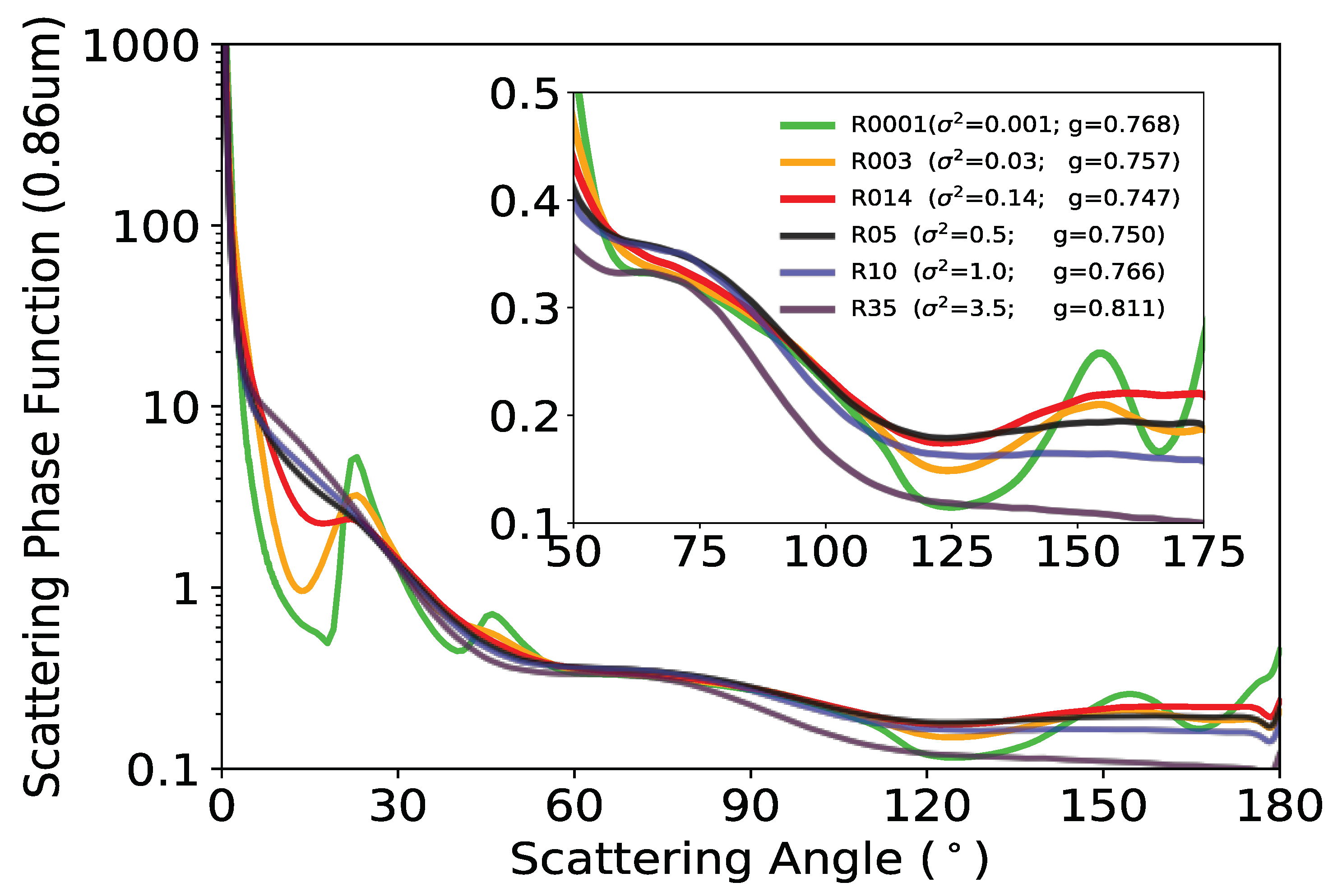
The MC6 roughened hexagonal ice aggregate model is used in the MODIS Collection 6 operational products [19], which assume ice cloud particles to be an ensemble of randomly oriented aggregates. Each aggregate is composed of eight hexagonal columns with a fixed degree of surface roughness σ² = 0.5. The roughness parameter σ² in the light scattering calculations is defined as the standard deviation of a two-dimensional Gaussian distribution for the tilting of a particle facet [20]. The standard deviation of this roughness parameter σ is approximately equivalent in value to the roughness parameter δ defined by Macke et al. [21,22,23]. A higher degree of roughness means a higher probability density of strongly distorted surfaces. Detailed descriptions of the ice particle habit and associated degree of surface roughness are discussed by Yang and Liou [20] and Yang et al. [24]. In general, the ice particle phase function at scattering angles between 50° and 175° becomes more featureless with an increasing degree of surface roughness (Figure 1) for six models assuming a range of surface roughness of σ² = 0.001, 0.03, 0.14, 0.5, 1.0, and 3.5 (hereafter, R0001, R003, R014, R05, R10, and R35, respectively). Note that the MC6 model corresponds to the R05 model. Both the ice particle habit and ice particle surface roughness can modify the single-scattering properties [25], although other factors are also important, such as particle impurities, internal fractures, and air bubbles. The asymmetry factor (g) for each model is also included in Figure 1. Among these selected models, the asymmetry factor decreases with an increasing degree of roughness until σ² = 0.14, beyond which the asymmetry factor increases in even rougher models. Perhaps some of this behavior in the most severely roughened models could be a modeling artifact associated with the ray-tracing technique when it is applied to a very rough particle surface. Although the MC6 ice particle habit model has a better match to global satellite measurements than other ice particle habits [1,4,26], the “optimal” degree of ice particle surface roughness for the MC6 ice model has not been studied rigorously yet. To test the degree of roughness used in MC6, we developed five other ice particle models using the MC6 ice particle habit, but with different degrees of ice particle surface roughness. The additional five degrees of roughness have different phase functions over the MISR observational range of scattering angles in comparison with the case of σ² = 0.5.

2.3. Look-Up Table Approach

LUTs are developed separately for each ice particle model, i.e., R0001, R003, R014, R05, R10, and R35. For each ice cloud particle model, the LUTs are calculated using an adding–doubling radiative transfer model [27]. The LUTs include model reflectances as a function of solar geometry, viewing geometry, and $\mathsf{\tau }$; the model reflectance $R$ is equivalent to the reflectance $\tilde{R}$ from MISR measurements in Equation (1). The bulk scattering properties for each ice particle model are the ensemble-mean single-scattering properties integrated over a Gamma distribution with an effective variance of 0.1 and an effective radius of 30 μm. The reflectance at wavelength 0.86 μm is insensitive to the particle effective size due to weak ice absorption. Atmospheric molecular scattering is considered in the model, but aerosols are neglected. The ocean surface reflection is based on the Cox-Munk model [28] with a wind speed of 10 m s⁻¹. The reflectance for each MISR camera is calculated by assuming a homogeneous cloud layer with a cloud-top pressure of 200 hPa. A sensitivity study shows that the effect of cloud-top pressure on retrievals is not substantial.

The $R$ values can be integrated over $\mu$ and $\varphi$ (viewing directions) to obtain the planetary albedo ($A_{\mathrm{p}}$):

$$A_p\left(P,{\mu }_0,{\varphi }_0,\tau \right)=\frac{1}{\pi }\underset{0}{\overset{2\pi }{{\displaystyle \int }}}\underset{0}{\overset{1}{{\displaystyle \int }}}R\left(P,{\mu }_0,{\varphi }_0,\tau \right)·\mu ·d\mu ·d\varphi$$

(2)

The cloud spherical albedo, $A_{\mathrm{s}},$ is the integration of $A_p$ over all incident directions (${\mu }_0,{\varphi }_0$):

$$A_s\left(P,\tau \right)=\frac{1}{\pi }\underset{0}{\overset{2\pi }{{\displaystyle \int }}}\underset{0}{\overset{1}{{\displaystyle \int }}}{A}_p\left(P,{\mu }_0,{\varphi }_0,\tau \right)·{\mu }_0·d{\mu }_0·d{\varphi }_0$$

(3)

By carrying out the integrals in Equations (2) and (3), $R$ is converted to $A_{\mathrm{s}}$ for a given $\tau$ in conjunction with a specific ice particle model. LUTs are developed for each ice particle model and contain both $R$ and the corresponding $A_{\mathrm{s}}$ as functions of $\tau$.

2.4. The SAD Method

The SAD method for examining angular variations of ice particle phase functions is described by Doutriaux-Boucher et al. [6] and C.-Labonnote et al. [29], who applied this method to POLDER data. These studies found that $A_{\mathrm{s}}$ has a one-to-one relationship with $\tau$ for a given ice particle model [6], implying that there is a one-to-one theoretical relationship between $A_{\mathrm{s}}$ and $\tilde{R}$. Because $R$ and $A_{\mathrm{s}}$ are provided in the LUTs, an $\tilde{R}$ value from each MISR camera measurement is used to search for the corresponding value of $R$ in the LUTs. The associated $A_{\mathrm{s}}$ in the LUTs is identified as the retrieved cloud spherical albedo ($\widetilde{A_{\mathrm{s}}}$) for this camera. This procedure is iteratively performed for every camera measurement to compute $\widetilde{A_{\mathrm{s}}}$. Because only three near-nadir cameras are selected from a set of MISR measurements, one cloudy pixel may correspond to 3 $\widetilde{A_{\mathrm{s}}}$ values.

Each MISR camera retrieves $\tilde{R}$ for a pixel at a different scattering angle ($\mathsf{\Theta }$). If an assumed ice particle model matches observations accurately over the range of three observed $\mathsf{\Theta }$ values, the model $R$ values would be equal to the observed $\tilde{R}$ values for every $\mathsf{\Theta }$. When $\tau$ is identical for all cameras, the same $\widetilde{A_{\mathrm{s}}}$ could be obtained. Given that idealized ice models may not fit a real cloud perfectly for every available $\mathsf{\Theta }$, there may be differences in the computed $\widetilde{A_{\mathrm{s}}}$ values. $A_{diff}$ is defined as the difference between the $\widetilde{A_{\mathrm{s}}}$ of a selected camera and the mean of $\widetilde{A_{\mathrm{s}}}$ averaged for the selected cameras for a given pixel:

$${[A_{diff}\left(P\right)]}_i={[{\tilde{A}}_s\left(P\right)]}_i-\frac{1}{n_c}{\displaystyle \sum }_{i=1}^{n_c}{[{\tilde{A}}_s\left(P\right)]}_i$$

(4)

where $i$ is the camera index in the pixel and $n_c$ is the total number of selected cameras in the given pixel. Because of the sun glint screening process, $n_c$ is not necessarily 3. As defined in Equations (2) and (3), $A_{\mathrm{s}}$ does not depend on either solar or viewing geometries but solely on P for a given $\tau$. Therefore, smaller absolute values of $A_{diff}$ indicate better consistency between simulations and observations.

To identify an optimal ice particle model, the same procedure is applied to each pixel using all LUTs. The smallest $A_{\mathrm{diff}}$ value from the six LUTs is chosen as the optimal model for that pixel. Finally, to quantify the consistency between ice particle models with observations, the standard deviation of $A_{\mathrm{diff}}$ (${\mathsf{\chi }}^2$) for each ice particle model in a given latitude bin is defined as follows:

$${\chi }^2{}_{{\sigma }^2}=\sqrt{\frac{1}{\left({{\displaystyle \sum }}_{k=1}^{n_b}{n}_R\right)}{\displaystyle \sum }_{k=1}^{n_b}{\displaystyle \sum }_{j=1}^{n_R}{\left[{\left(A_{diff}\right)}_{j,k}\right]}^2}$$

(5)

where $n_R$ is the total number of selected reflectances in a latitude-scattering angle bin and $n_b$ is the total number of selected latitude-scattering angle bins in a particular latitude band.

3. Results

3.1. Sampling Scattering Geometry Characteristics

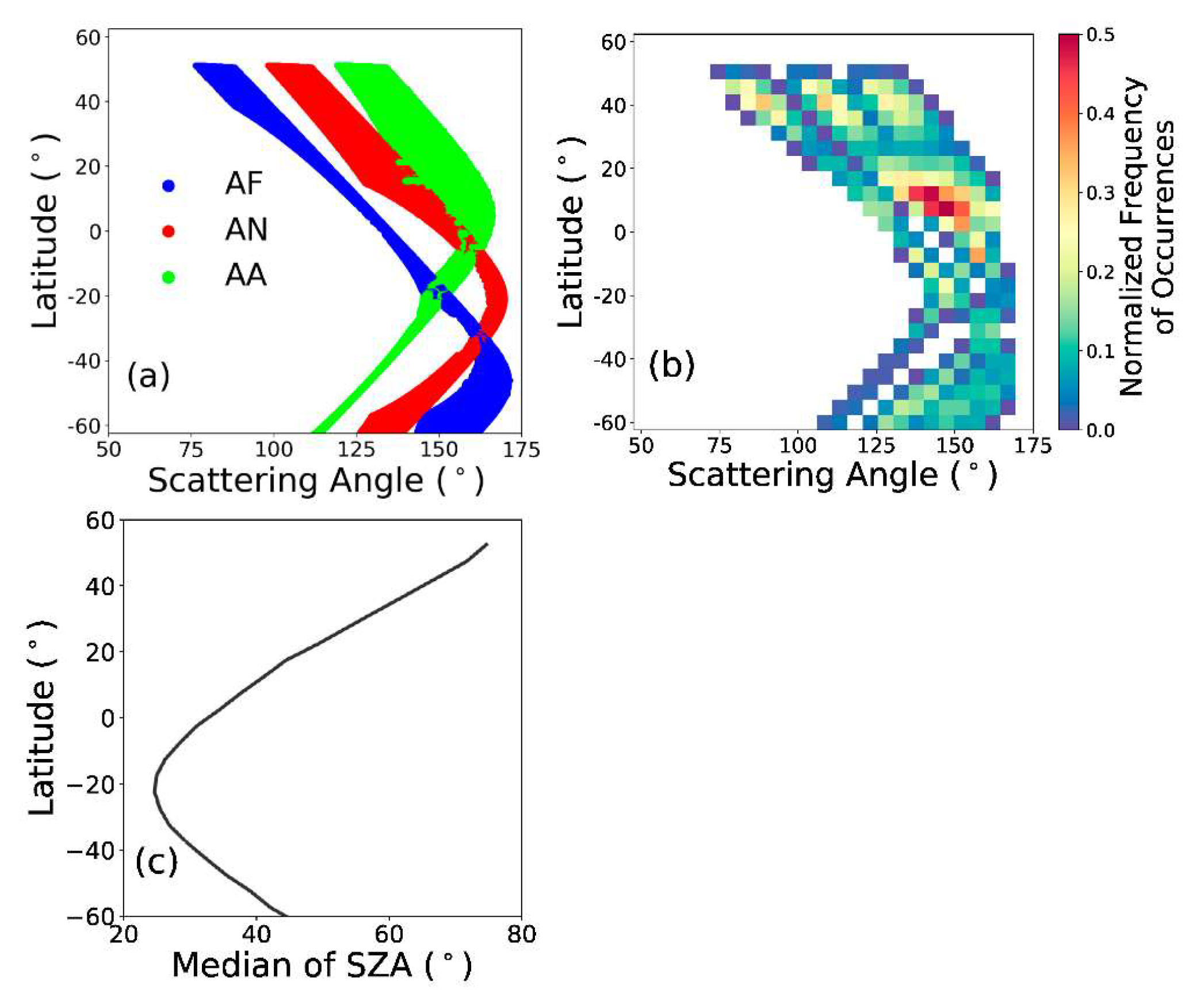
Figure 2a,b show the MISR camera names that are used and the normalized frequency of occurrences of $\mathsf{\Theta }$ and latitude based on the four chosen December solstice days during 2012–2015 from the MISR-MODIS fused dataset over oceans. Due to the varying SZA with latitude and different VZAs of each MISR camera, the cameras provide reflectances at different $\mathsf{\Theta }$ for a given pixel, and the $\mathsf{\Theta }$ changes with latitude. The minimum available $\mathsf{\Theta }$ is 76° and the maximum available $\mathsf{\Theta }$ is 172° in these selected pixels. Because the daytime orbit of the Terra satellite is from north to south with an equator crossing time at 10:30 am, the forward camera measures at smaller $\mathsf{\Theta }$ than the aft camera in the northern high latitudes. The three cameras primarily take measurements in the side and backward scattering directions. Note that the presence of arc-shaped strips in Figure 2a is a result of filtering out the pixels with sun glint. For the same reason, some bins in Figure 2b have no observations.

The detected range of $\mathsf{\Theta }$ changes with latitude, in large part due to changes in SZA, as shown in Figure 2c. The camera geometry discussed above causes the detected range of $\mathsf{\Theta }$ variation with SZA. The narrowest range of scattering angle measurements occurs at the lowest SZA (~20° S), where no reflectances are measured at $\mathsf{\Theta }$ < 140°. However, all reflectances are measured at $\mathsf{\Theta }$ < 140° at the highest SZA (~50°–60° N). The latitudes where measurements are made at the largest $\mathsf{\Theta }$ are different for each camera, but roughly speaking, all three cameras measure in side scattering to backscattering directions with increasing SZA. The frequencies of Θ observations also reveal latitudinal variations. When the SZA is low, the same scattering angles can be recorded by two cameras viewing the same pixel.

3.2. Latitudinal Variations in Consistency between Ice Models and Observations

3.2.1. Consistency of Models and Measurements with Latitude

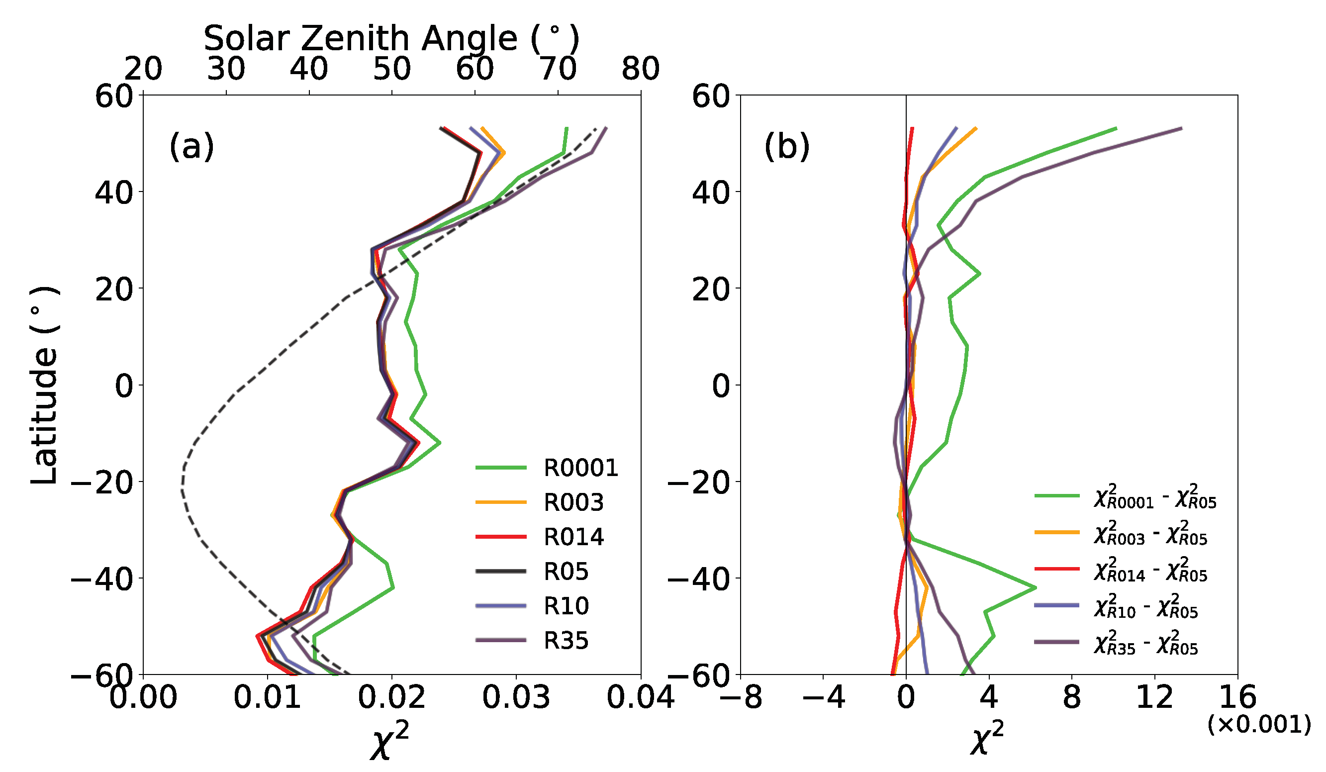
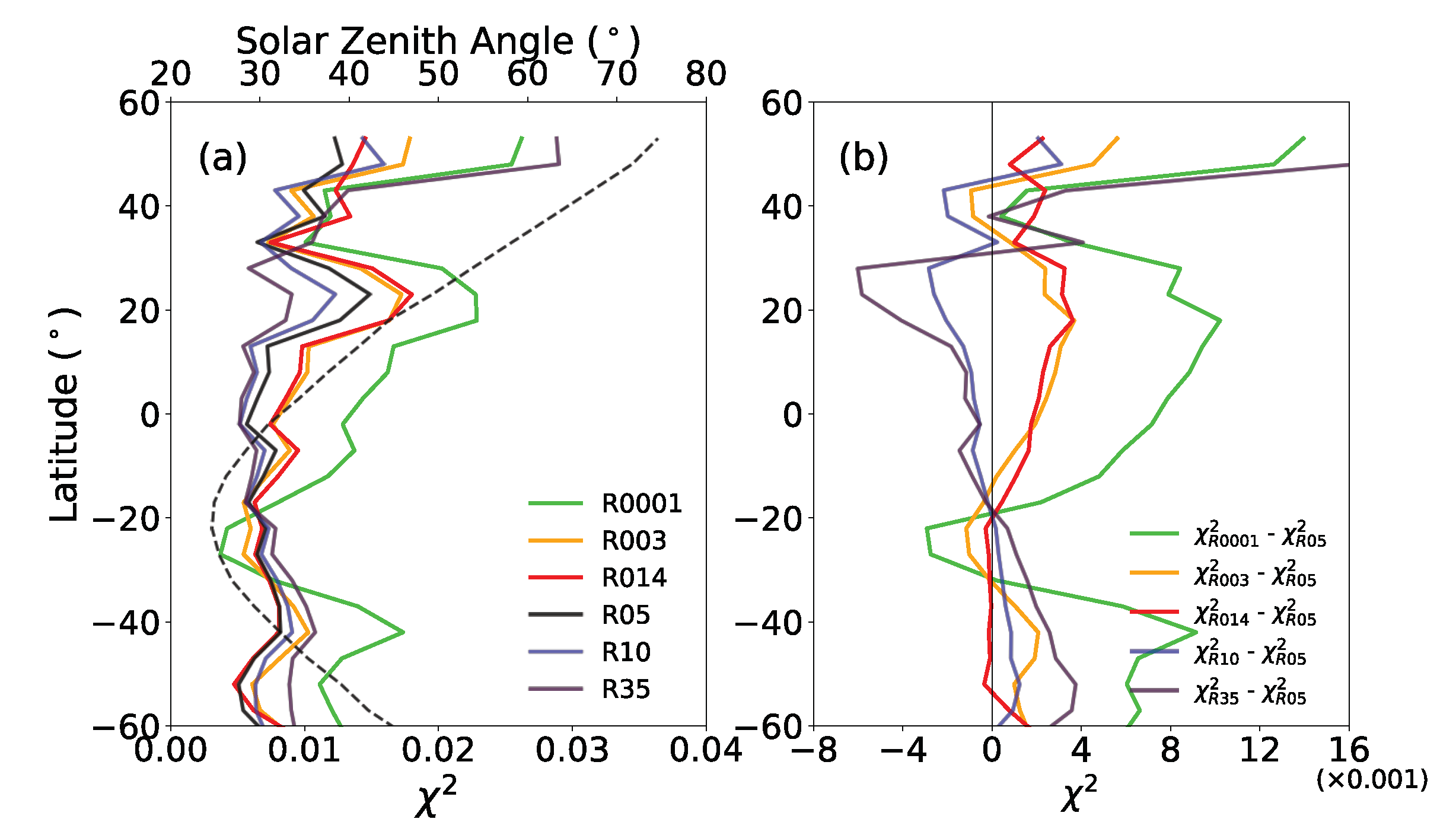
The quantity ${\mathsf{\chi }}^2$ in Equation (5) as a function of latitude for each particle model is shown in Figure 3a, and quantitative comparisons between the R05 and other models based on Equation (5) are displayed in Figure 3b. The ${\mathsf{\chi }}^2$ values for all models in the Northern Hemisphere are larger than in the Southern Hemisphere and decrease with latitude from north to south. The six ${\mathsf{\chi }}^2$ values are more similar in value to each other in the low latitudes than in the high latitudes of both hemispheres. Figure 3 shows that the R05 and R014 models have similar ${\mathsf{\chi }}^2$ values over the latitude range, and both models have lower ${\mathsf{\chi }}^2$ values than the other models in all latitudes. Note that these two models have lower g than the other models (Figure 1). However, the relationships between ${\mathsf{\chi }}^2$ and g are not simple. The R35 model has the highest g but has a lower ${\mathsf{\chi }}^2$ value than the R0001 model in most latitudes. Also, the R0001 and R10 models have similar g values, but the consistency of $A_{\mathrm{diff}}$ results for the R0001 model is much less than in the case of the R10 model.

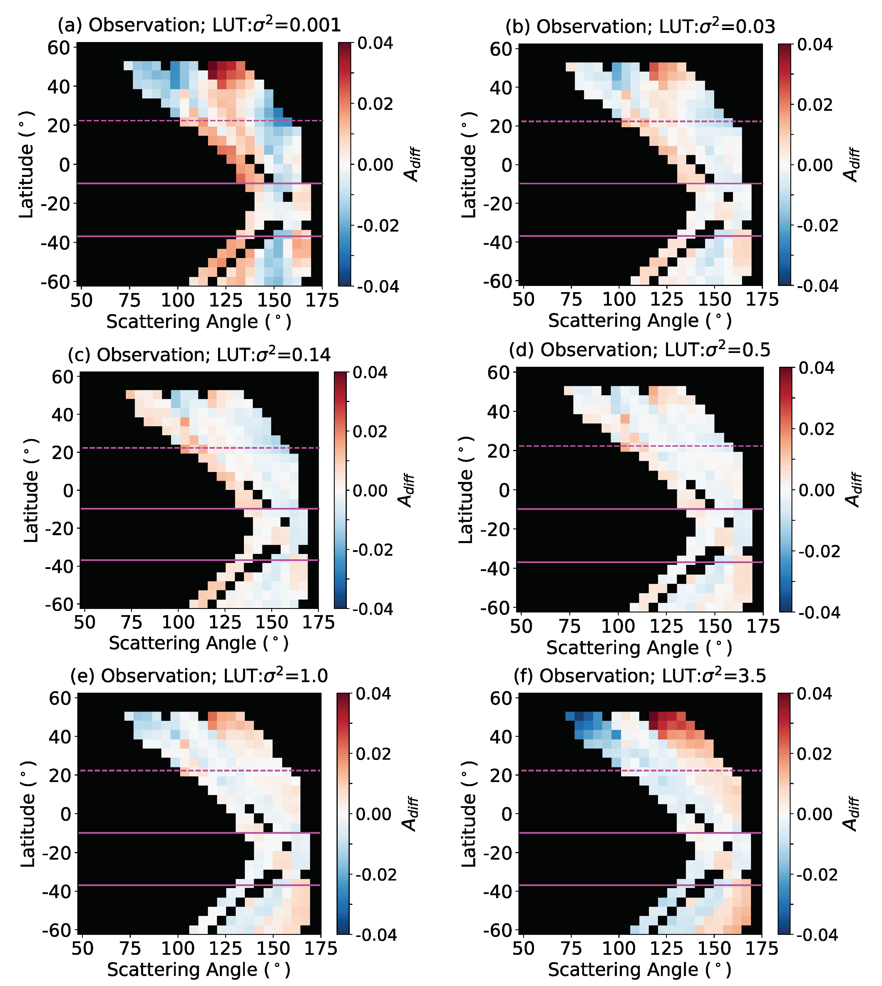
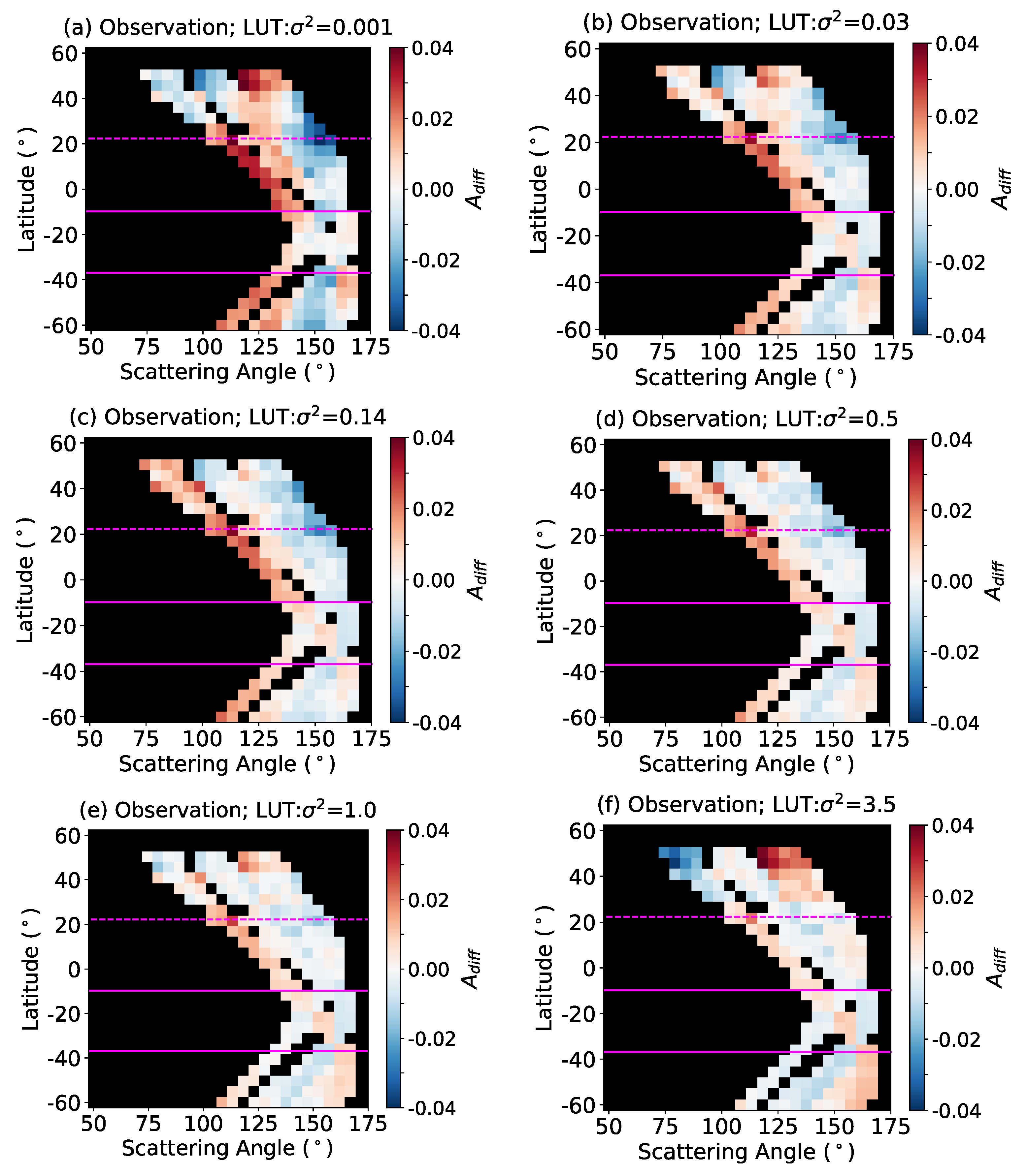
To better understand the contributions of $A_{\mathrm{diff}}$ to ${\mathsf{\chi }}^2$, Figure 4 shows the median value of $A_{\mathrm{diff}}$ (hereafter, $A_{\mathrm{diff}}$ indicates the median value in 5° $\times$ 5° latitude-$\mathsf{\Theta }$ bins) on December solstices during 2012–2015. The variations of $A_{\mathrm{diff}}$ values more closely follow the changes in SZA. The axis of symmetry of $A_{\mathrm{diff}}$ is located at about 20° S, where there is a minimum in the $\mathsf{\Theta }$ range. For SZA < 30°, the $A_{\mathrm{diff}}$ values computed with all six models display nearly the same pattern. The $A_{\mathrm{diff}}$ values are close to zero for most $\mathsf{\Theta }$, but slightly negative at the highest $\mathsf{\Theta }$ ($\mathsf{\Theta }$~170°). As SZA increases, $A_{\mathrm{diff}}$ values are still close to zero when 30° < SZA < 50°. However, $A_{\mathrm{diff}}$ values become positive for the largest measurable $\mathsf{\Theta }$ with an increasing degree of roughness and become negative for the smallest measurable $\mathsf{\Theta }$ with a decreasing degree of roughness. At high latitudes (SZA > 50°), the $A_{\mathrm{diff}}$ values broadly become highly positive or negative as shown in Figure 4a,b,e,f (especially in Figure 4a,f), but not in Figure 4c,d. The absence of large extreme values at high latitudes in Figure 4c,d indicate that the R014 and R05 models have lower ${\mathsf{\chi }}^2$ values than the other models in high latitudes in Figure 3. Some of the latitudinal $A_{\mathrm{diff}}$ value differences could be a result of the change of measurable $\mathsf{\Theta }$ as shown in Figure 2a. Another issue that might influence the results is incomplete filtering of sun glint regions. Note that Figure 4a has significantly negative $A_{\mathrm{diff}}$ values in most latitudes at $\mathsf{\Theta }$~150° where the phase function of the R0001 model has an obvious peak in Figure 1. In general, the consistency of $A_{diff}$ results for the R05 and R014 models is better than for the other models in high latitudes, and similar in the tropics.

3.2.2. Sensitivity Test with Synthetic Dataset

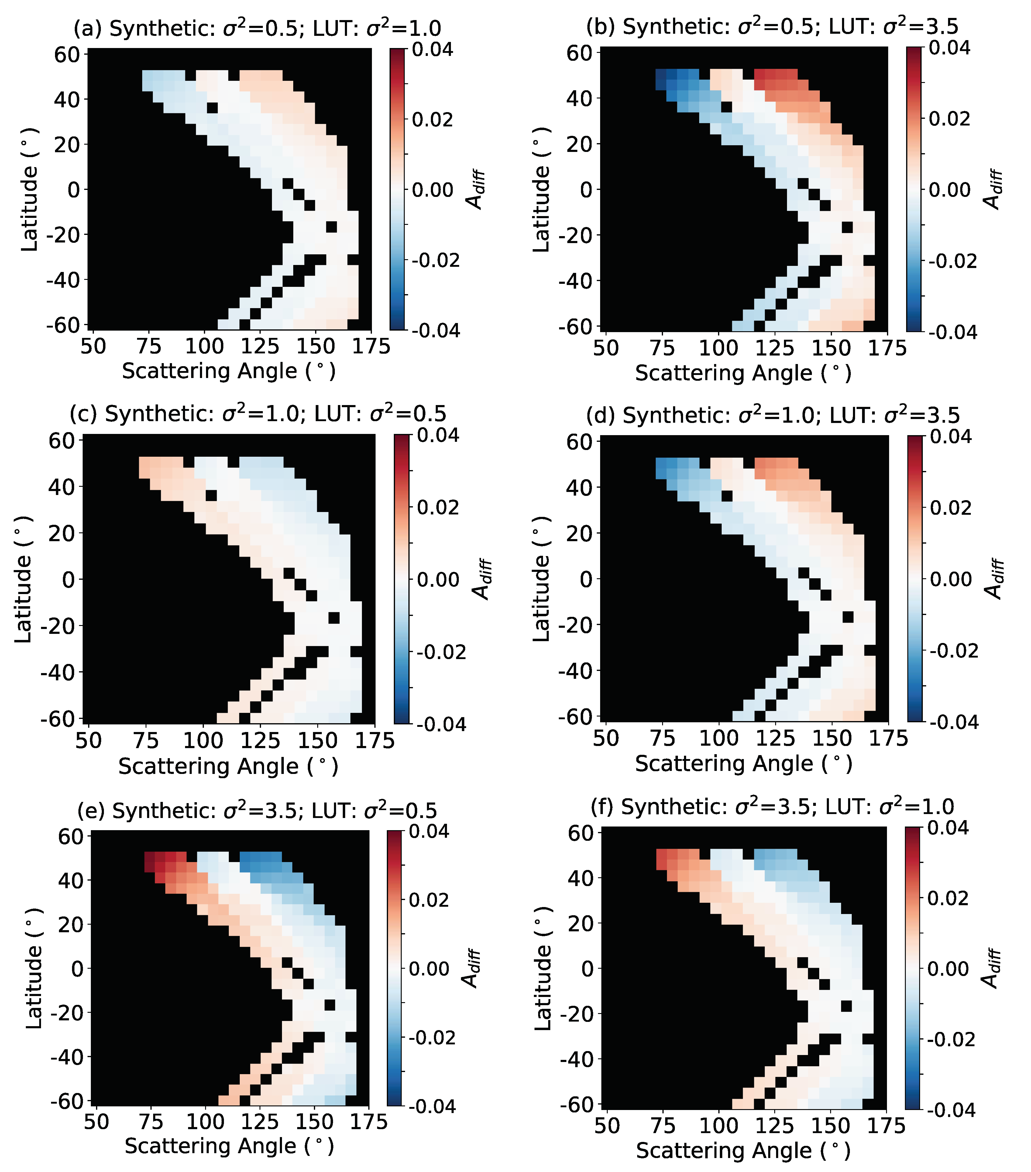
To investigate which ice particle model produced $A_{\mathrm{diff}}$ values at high SZAs such as the case shown in Figure 4, a sensitivity study is performed with simulated data (Figure 5). The simulated radiances are generated using the same December solstice observations and the same pixel filtering process as in Section 2.1, the viewing geometry from each MISR camera observation, and the $\mathsf{\tau }$ from MODIS with the R05, R10, and R35 models. In other words, the simulated radiances are constructed using the same satellite geometry as the MISR data but the reflectances are generated with the R05, R10, and R35 model LUTs using the $\tau$ from the collocated MODIS MC6 product. Subsequently, $A_{\mathrm{diff}}$ values are computed using the LUTs from the other two ice particle models.

Compared to the simulated dataset produced by the R10 model (Figure 5c,d) and the R35 model (Figure 5e,f), $A_{\mathrm{diff}}$ values computed from the simulated dataset produced by the R05 model (Figure 5a,b) have better consistency with $A_{\mathrm{diff}}$ values computed with real data (Figure 4) at high SZAs. Specifically, Figure 5a and Figure 4e illustrate $A_{\mathrm{diff}}$ values based on the same R10 LUTs. The simulated $A_{\mathrm{diff}}$ pattern in Figure 5a reproduces the negative–positive patterns of $A_{\mathrm{diff}}$ values (i.e., positive values of $A_{\mathrm{diff}}$ become negative with increasing $\mathsf{\Theta }$ in a latitude) at high latitudes in Figure 4e. Similar negative–positive patterns in high latitudes are seen in both Figure 4f and Figure 5b, which use the same R35 LUTs. However, neither Figure 5d nor Figure 5f are similar to Figure 4f even using the same R35 LUTs. The similarity of using the same LUTs between Figure 4 and Figure 5 indicate that the R05 model is closer to the actual ice particle in the measurable range of scattering angles at high latitudes. With use of the same approach to compare Figure 4 and Figure 5 under SZA < 30°, it is found that both the R05 and R10 models do not match the actual ice cloud particle as well as the R35 model when SZA < 30°, but the difference with the R35 results are rather small. To summarize, the similarity between Figure 4 and Figure 5 implies that the R05 model fits observations better than the R10 and R35 models for SZA > 30°. However, it is not straightforward to select the most optimal model when SZA < 30°.

3.2.3. Classification by Heterogeneity of Clouds

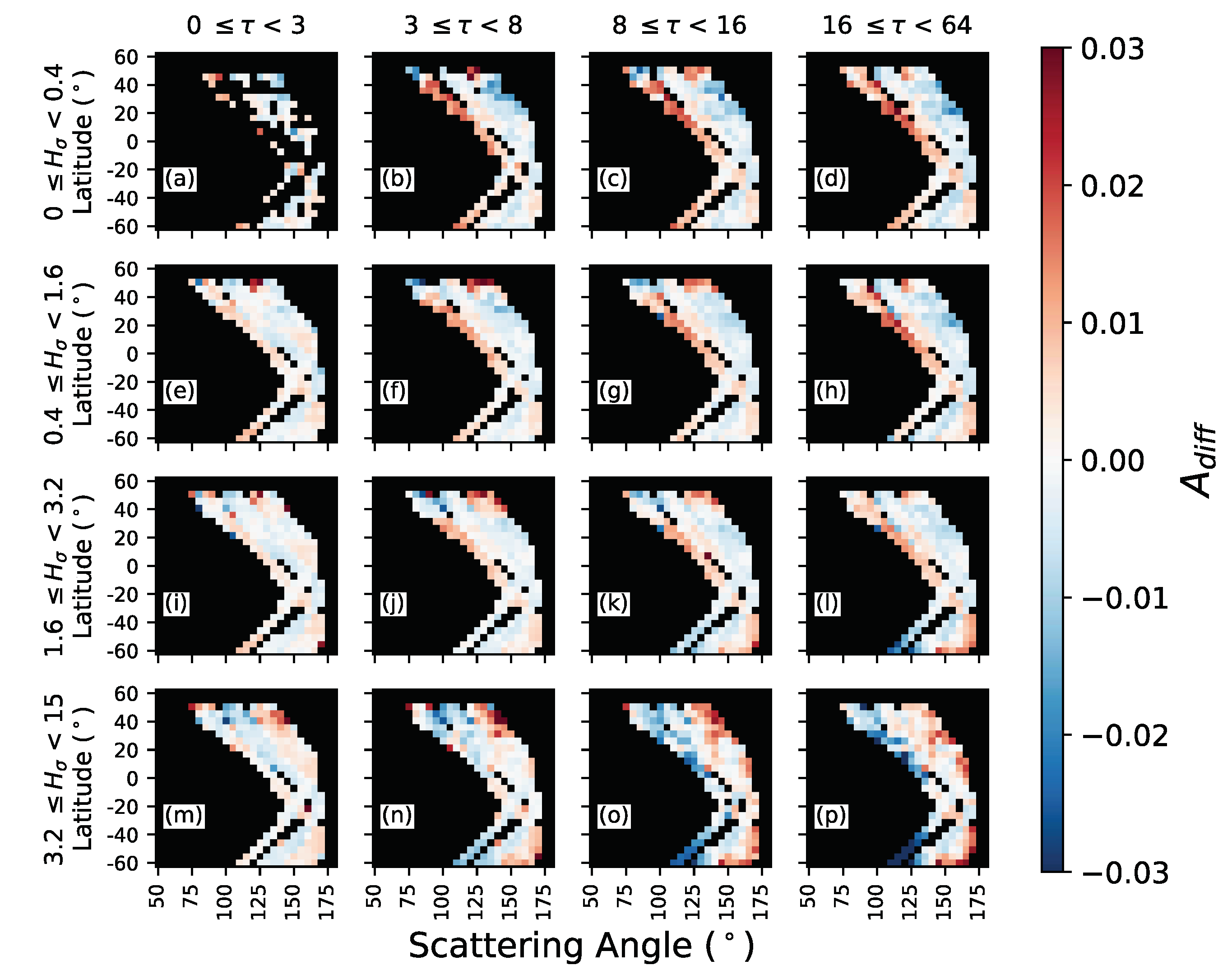
To better understand the effect of cloud heterogeneity on variations of $A_{\mathrm{diff}}$ values in latitude, we further classify the $A_{\mathrm{diff}}$ values by $H_{\mathsf{\sigma }}$ and $\tau$. Figure 6 shows $A_{\mathrm{diff}}$ computed with the R05 model in a 4 $\times$ 4 matrix with four $\tau$ bins: 0–3, 3–8, 8–16, and 16–64, and four $H_{\mathsf{\sigma }}$ bins: <0.4, 0.4–1.6, 1.6–3.2, and 3.2–15. A previous study [30] selected 0.3 as the threshold for a homogenous cloud, but very few selected pixels in this study meet this threshold. Therefore, a higher threshold (i.e., $H_{\mathsf{\sigma }}$ = 0.4) was used here to select homogeneous clouds (i.e., the first row in Figure 6). The same pixel filtering process as in Section 2.1 was applied here.

The $A_{\mathrm{diff}}$ values become more negative or more positive with increasing $\tau$ in Figure 6. The larger absolute value of $A_{\mathrm{diff}}$ for larger $\tau$ show the R05 results are more consistent with measurements for optically thin clouds than in optically thick clouds. Unlike the impact of increasing $\mathsf{\tau }$, the sign of $A_{\mathrm{diff}}$ changes with increasing $H_{\mathsf{\sigma }}$. In a broad sense, $A_{\mathrm{diff}}$ decreases with increasing $\mathsf{\Theta }$ in low $H_{\mathsf{\sigma }}$ bins but increases with increasing $\mathsf{\Theta }$ in high $H_{\mathsf{\sigma }}$ bins. Compared with all $H_{\mathsf{\sigma }}$ bins, $1.6<H_{\mathsf{\sigma }}<3.2$ bins have a trend of $A_{\mathrm{diff}}$ with increasing $\mathsf{\Theta }$ that is similar to the trend in Figure 4a. When $H_{\mathsf{\sigma }}$ increases, the decreasing trend of $A_{\mathrm{diff}}$ values with increasing $\mathsf{\Theta }$ reverses to an increasing trend, indicating that the scattering angular distribution of reflectance depends on cloud homogeneity.

3.2.4. Latitudinal Variations of Consistency in Measurements of Thick Homogeneous Clouds

Since low $H_{\mathsf{\sigma }}$ clouds are less likely to be influenced by 3D effects, the results are recomputed for thick homogeneous clouds ($H_{\mathsf{\sigma }}$ < 0.4 and $\mathsf{\tau }$ > 16). Figure 7 and Figure 8 are the same as Figure 3 and Figure 4, but only for thick homogeneous clouds. Compared to the results for global clouds (Figure 3), the results for thick homogeneous clouds show that: (1) the ${\mathsf{\chi }}^2$ of all selected models are significantly lower in thick homogeneous clouds; (2) the absolute differences of ${\mathsf{\chi }}^2$ among models are much larger in both the tropics and extra-tropics; and (3) the ${\mathsf{\chi }}^2$ of each model in the Northern Hemisphere is not significantly larger than ${\mathsf{\chi }}^2$ in the Southern Hemisphere. While the R05 model generally has the lowest ${\mathsf{\chi }}^2$ in all latitudes in Figure 3, the ${\mathsf{\chi }}_{\mathrm{R}10}^2$ and ${\mathsf{\chi }}_{\mathrm{R}35}^2$ results are smaller than the ${\mathsf{\chi }}_{\mathrm{R}05}^2$ counterparts at latitudes between 20° S and 30° N in Figure 7. In latitudes between 20° S–60° S and between 30° N–60° N, the R05 model and the less roughened ice models produce better fits among the six. In other words, the optimal model suggests the need for rougher ice particles in the tropics than in the extra-tropics. Furthermore, Figure 7 does not show a simple relationship between ${\mathsf{\chi }}^2$ and g. For instance, at latitudes between 20° S and 30° N, ${\mathsf{\chi }}^2$ of the R14 model, which has the lowest g, is within the range of the other models, and ${\mathsf{\chi }}^2$ of the R0001 and R35 models are not similar even though these two models have similar g values.

Figure 8 is the same as Figure 4 but computed for thick homogeneous clouds ($H_{\mathsf{\sigma }}$ < 0.4 and $\tau$ > 16). For SZA < 30°, the $A_{\mathrm{diff}}$ values computed with all six models display nearly the same pattern as shown in Figure 4, and values are close to zero at most measurable scattering angles. Every model in Figure 8 shows positive $A_{\mathrm{diff}}$ values for the lowest measurable $\mathsf{\Theta }$ in each latitude when 30° < SZA < 50°, particularly with less roughened models. At high latitudes (SZA > 50°), the $A_{\mathrm{diff}}$ values show a relationship with g. Specifically, the $A_{\mathrm{diff}}$ values at the smallest measurable $\mathsf{\Theta }$ turn negative with a higher g model and at the largest measurable $\mathsf{\Theta }$ turn positive.

4. Discussion

To examine the latitudinal variations of six ice particle models with a range of surface roughness, we compute spherical albedo difference ($A_{\mathrm{diff}}$) values using different LUTs for each model. We then compute the ${\mathsf{\chi }}^2$ (the residual sum of squares of mean $A_{\mathrm{diff}}$) in latitude. The $A_{\mathrm{diff}}$ is defined as the difference between the cloud spherical albedo ($\widetilde{A_{\mathrm{s}}}$) of a selected MISR camera and the mean of $\widetilde{A_{\mathrm{s}}}$ averaged across all available cameras for a given pixel. The ${\mathsf{\chi }}^2$ values in the extra-tropics are significantly larger than the counterparts in the tropics. Hexagonal column ice particles occur more frequently at low latitudes than high latitudes [31], and this may be a possible reason that the aggregated hexagonal column habit better explains the ice particle in the tropics than in the extra-tropics. The differences of ${\mathsf{\chi }}^2$ values among ice models in the global data are not significant in the tropics, and MISR data are unable to discriminate between the models. However, in the thick homogeneous cloud regime, the differences of ${\mathsf{\chi }}^2$ values among models were significantly heightened in both the tropics and extra-tropics. The optimal particles are more roughened in the tropics than in the extra-tropics in thick homogeneous clouds, which is in agreement with previous results [4]. The high frequency of strong convection in the tropics likely has an influence on the MISR observations, leading to an indication of heightened surface roughening.

In addition to the ${\mathsf{\chi }}^2$ variation with latitude, the variation of $A_{\mathrm{diff}}$ as a function of increasing scattering angle $\mathsf{\Theta }$ also varies with latitude but more precisely changes with SZA when using any of the LUTs. These differences of $A_{\mathrm{diff}}$ also appear in the clouds stratified by cloud homogeneity index $H_{\mathsf{\sigma }}$ and optical thickness $\tau$. If a given camera-retrieved $\tau$ is higher than the counterparts associated with the other cameras, a higher $A_{\mathrm{s}}$ value would be computed for this one camera than for the other cameras, and this higher $A_{\mathrm{s}}$ value leads to a positive $A_{\mathrm{diff}}$ value. Therefore, the magnitudes of $A_{\mathrm{diff}}$ values at different $\mathsf{\Theta }$ imply differences between the retrieved $\tau$ and the mean $\tau$ of all cameras in each $\mathsf{\Theta }$. A positive (negative) $A_{\mathrm{diff}}$ value broadly means that the retrieved $\tau$ is larger (smaller) than mean $\tau$ of all cameras. Furthermore, the inference of $\tau$ is determined primarily by phase function, and the impact of ice particle phase function on reflectance is important [32,33], particularly for optically thin clouds. Thus, the sign of the $A_{\mathrm{diff}}$ value is related to the variation of the phase function with a scattering angle. Note that the $A_{\mathrm{diff}}$ method is not sensitive to the absolute value of the phase function, but only to the relative variation of the phase function with scattering angle. This approach, also described in C.-Labonnote et al. [32], is able to explain why the $A_{\mathrm{diff}}$ value at $\mathsf{\Theta }$. ~150° in Figure 4a is negative at almost every latitude, but this difference does not appear in other panels in Figure 4 because the phase function of the R0001 model has a significant peak at $\mathsf{\Theta }$~150°. Similarly, this is the reason that the R05 model fits the measurements better than the other models at most latitudes. The phase function of the R05 model fits the measurements better than the other selected models over the MISR available $\mathsf{\Theta }$ range.

High latitudes tend to have a high SZA, and the 3D radiative effect is one potential explanation for how the $A_{\mathrm{diff}}$ appears to change with SZA. Previous studies [15,34,35] investigate the impact of solar geometry on the 3D effect, particularly variations of the retrieved $\mathsf{\tau }$ with SZA. Since $\tau$ can easily be converted to $A_{\mathrm{s}}$, there may be a similar potential impact of the 3D effect on the results. In general, low $H_{\mathsf{\sigma }}$ clouds have uniform cloud tops, which approximately satisfy the plane-parallel approximation. Thus, the impact of the 3D effect on reflectance of this type of cloud is not as strong as on a high $H_{\mathsf{\sigma }}$ cloud. Therefore, low $H_{\mathsf{\sigma }}$ clouds are usually less susceptible to the 3D effect than high $H_{\mathsf{\sigma }}$ clouds. The stratified clouds in Figure 6 have better agreement with this theory. The trend of $A_{\mathrm{diff}}$ values with increasing $\mathsf{\Theta }$ as a function of SZA is significantly larger for high $H_{\mathsf{\sigma }}$ clouds than for low $H_{\mathsf{\sigma }}$ clouds. Note that we consider only one definition of cloud heterogeneity, and a different definition may lead to different results [36].

The microphysical ice particle habit distribution changes with latitude, dynamical environment, and temperature [37,38,39] could impact the trend of $A_{\mathrm{diff}}$ values with increasing $\mathsf{\Theta }$ at different latitudes as well. In the thick homogeneous cloud regime (Figure 8), not all models show different trends of $A_{\mathrm{diff}}$ values with $\mathsf{\Theta }$ in different latitudes compared to global clouds (Figure 4). In addition, high latitudes frequently have ice clouds with a lower cloud top height [40]. If we remove clouds with cloud-top temperatures >233K in the data filtering process, some ice clouds at high latitudes are probably removed because the tropopause is lower there. It is interesting to note that for the thick homogeneous cloud regime, the larger differences of ${\mathsf{\chi }}^2$ values between the models enable some discrimination between values of surface roughness. The best-fit particles are more roughened in the tropics than extra-tropics in thick homogeneous clouds.

The limited and variable range of available $\mathsf{\Theta }$ measurements might be one source of uncertainty for computing the $A_{\mathrm{diff}}$ value. Only limited $\mathsf{\Theta }$ ranges can be sampled by the MISR sensor, but the whole $\mathsf{\Theta }$ range must be used in retrievals to compute reflectance. It means that there is insufficient data to know how the phase function in the undetectable $\mathsf{\Theta }$ range changes in each latitude, and to evaluate how large the influence of the phase function in the undetectable $\mathsf{\Theta }$ are to our results. The range of available $\mathsf{\Theta }$ values from MISR varies systematically with SZA (Figure 2). McFarlane and Marchand [26] also suggested that the retrieved ice particle habit depends on the minimum observed $\mathsf{\Theta }$. Not only the $\mathsf{\Theta }$ range but also the pixel frequencies in each $\mathsf{\Theta }$—latitude bin changes with latitude. Because of varying sun-earth-satellite viewing geometry, it is not straightforward to evaluate these factors on the computed $A_{\mathrm{diff}}$ value.

The consistency of six ice models (R0001, R003, R014, R05, R10, and R35 model) is compared to MISR measurements at different latitudes. Our results, based on the fused MODIS-MISR dataset, can be used to estimate the latitudinal (or SZA) bias in retrievals of MC6 operational products because the MC6 operational ice cloud property retrievals assume that the same R05 model applies globally. Our analysis shows that the R05 model works very consistently with global MISR measurements but there may need to be more roughened particles in the tropics.

In the bi-spectral shortwave technique [41], a large asymmetry factor ice particle model causes a higher retrieved $\tau$ and lower r_eff [42]. The asymmetry factors of the R05 and R014 models are the lowest of the six models, and the R35 model has the largest asymmetry factor. As noted earlier, the extreme randomly distorted particle surface facets of the R35 model may increase the amount of forward scattering as an artifact of the numerical modeling. Since the best-fit model is hard to define in the tropics because of the rather small differences in ${\mathsf{\chi }}^2$ values, the ice cloud $\tau$ and effective radius could have large uncertainties by assuming the best-fit model from MISR measurements in the retrieval.

5. Summary and Conclusions

This study examines the latitudinal dependence of ice particle models, based on the MISR-MODIS fused dataset on December solstices from 2012 to 2015. To evaluate the latitudinal consistency of ice particle models with MISR measurements, we apply the SAD method to the fused dataset by using the ice particle habit of the MODIS Collection 6 (MC6) ice model (R05 model) with six different assumptions of ice particle surface roughness: σ² = 0.001, 0.03, 0.14, 0.5, 1.0, and 3.5 (referred to as R0001, R003, R014, R05, R10, and R35 models, respectively).

Of the six models used in this study, the R05 model is one of the most consistent in comparison with the MISR measurements globally but has a similar consistency with other models at lower latitudes. The results of computing the residual sum of squares of mean $A_{\mathrm{diff}}$ (${\mathsf{\chi }}^2$) show that all six ${\mathsf{\chi }}^2$ are much higher at >30°N than all other latitudes. For thick homogeneous clouds, the consistency among models is significantly greater in both the tropics and extra-tropics, and the larger differences of ${\mathsf{\chi }}^2$ values between the models enable some discrimination between values of surface roughness. The optimal particle model should have rougher ice particles in the tropics than in the extra-tropics. Specifically, the MC6 model and less roughened models fit thick homogeneous clouds better than more roughened models in the zonal means for latitudes between 20°S–60°S and 30°N–60°N; for latitudes between 20°S and 30°N, more roughened models produce better fits among the six.

Comparisons of computed $A_{diff}$ values in latitude bands show that the trend of $A_{diff}$ values with increasing $\mathsf{\Theta }$ for each ice model changes with latitude, or more precisely, these variations are primarily a function of SZA. This result demonstrates the latitudinal variation of the best-fit model because of the relationship between SZA and latitude (e.g., the SZA in high latitudes is large). The variation of $A_{diff}$ values with $\mathsf{\Theta }$ also appears to change with SZA. However, homogenous clouds (low $H_{\mathsf{\sigma }}$ values) do not show the change of $A_{diff}$ trend with SZA. In addition, for the classified results, the sign of $A_{diff}$ changes with increasing $H_{\mathsf{\sigma }}$, but not with increasing $\tau$, as only the magnitudes of the $A_{diff}$ values increase with increasing $\tau$.

Because MISR provides reflectances over a wider $\mathsf{\Theta }$ range than MODIS, the collocated MODIS and MISR data/products provide an unprecedented opportunity to identify the optimal ice particle model for retrievals. The variations of the ${\mathsf{\chi }}^2$ value with latitude found in this study suggest that the invariant ice particle shape assumption for retrieving ice particle properties needs to be reconsidered.

References

- Holz, R.E.; Platnick, S.; Meyer, K.; Vaughan, M.; Heidinger, A.; Yang, P.; Wind, G.; Dutcher, S.; Ackerman, S.; Amarasinghe, N.; et al. Resolving ice cloud optical thickness biases between CALIOP and MODIS using infrared retrievals. Atmos. Chem. Phys. 2016, 16, 5075–5090. [Google Scholar] [CrossRef] [Green Version]
- Platnick, S.; Meyer, K.; King, M.D.; Wind, G.; Amarasinghe, N.; Marchant, B.; Arnold, G.T.; Zhang, Z.; Hubanks, P.A.; Holz, R.E.; et al. The MODIS cloud optical and microphysical products: Collection 6 updates and examples from Terra and Aqua. IEEE Trans. Geosci. Remote Sens. 2017, 55, 502–525. [Google Scholar] [CrossRef] [PubMed]
- Letu, H.; Ishimoto, H.; Riedi, J.; Nakajima, T.Y.; Labonnote, L.C.; Baran, A.J.; Nagao, T.M.; Sekiguchi, M. Investigation of ice particle habits to be used for ice cloud remote sensing for the GCOM-C satellite mission. Atmos. Chem. Phys. 2016, 16, 12287–12303. [Google Scholar] [CrossRef] [Green Version]
- Cole, B.H.; Yang, P.; Baum, B.A.; Riedi, J.; C-Labonnote, L. Ice particle habit and surface roughness derived from PARASOL polarization measurements. Atmos. Chem. Phys. 2014, 14, 3739–3750. [Google Scholar] [CrossRef] [Green Version]
- Hioki, S.; Yang, P.; Baum, B.A.; Platnick, S.; Meyer, K.G.; King, M.D.; Riedi, J. Degree of ice particle surface roughness inferred from polarimetric observations. Atmos. Chem. Phys. 2016, 16, 7545–7558. [Google Scholar] [CrossRef] [Green Version]
- Doutriaux-Boucher, M.; Buriez, J.C.; Brogniez, G.; Labonnote, L.C.; Baran, A.J. Sensitivity of retrieved POLDER directional cloud optical thickness to various ice particle models. Geophys. Res. Lett. 2000, 27, 109–112. [Google Scholar] [CrossRef]
- McFarlane, S.A.; Marchand, R.T.; Ackerman, T.P. Retrieval of cloud phase and crystal habit from Multiangle Imaging Spectroradiometer (MISR) and Moderate Resolution Imaging Spectroradiometer (MODIS) data. J. Geophys. Res. 2005, 110, D14201. [Google Scholar] [CrossRef]
- Sun, W.B.; Loeb, N.G.; Yang, P. On the retrieval of ice cloud particle shapes from POLDER measurements. J. Quant. Spectrosc. Radiat. Transf. 2006, 101, 435–447. [Google Scholar] [CrossRef]
- Xie, Y.; Yang, P.; Kattawar, G.W.; Minnis, P.; Hu, Y.X.; Wu, D.L. Determination of ice cloud models using MODIS and MISR data. Int. J. Remote Sens. 2012, 33, 4219–4253. [Google Scholar] [CrossRef]
- Wang, C.X.; Yang, P.; Dessler, A.; Baum, B.A.; Hu, Y.X. Estimation of the cirrus cloud scattering phase function from satellite observations. J. Quant. Spectrosc. Radiat. Transf. 2014, 138, 36–49. [Google Scholar] [CrossRef]
- Baran, A.J.; Francis, P.N.; Labonnote, L.C.; Doutriaux-Boucher, M. A scattering phase function for ice cloud: Tests of applicability using aircraft and satellite multi-angle multi-wavelength radiance measurements of cirrus. Q. J. R. Meteorol. Soc. 2001, 127, 2395–2416. [Google Scholar] [CrossRef]
- Baran, A.J.; Labonnote, L.C. On the reflection and polarisation properties of ice cloud. J. Quant. Spectrosc. Radiat. Transf. 2006, 100, 41–54. [Google Scholar] [CrossRef]
- Baran, A.J.; Labonnote, L.C. A self-consistent scattering model for cirrus. I: The solar region. Q. J. R. Meteorol. Soc. 2007, 133, 1899–1912. [Google Scholar] [CrossRef] [Green Version]
- Liang, L.S.; Di Girolamo, L.; Platnick, S. View-angle consistency in reflectance, optical thickness and spherical albedo of marine water-clouds over the northeastern Pacific through MISR-MODIS fusion. Geophys. Res. Lett. 2009, 36, L09811. [Google Scholar] [CrossRef]
- Liang, L.S.; Di Girolamo, L. A global analysis on the view-angle dependence of plane-parallel oceanic liquid water cloud optical thickness using data synergy from MISR and MODIS. J. Geophys. Res. 2013, 118, 2389–2403. [Google Scholar] [CrossRef] [Green Version]
- Diner, D.J.; Beckert, J.C.; Reilly, T.H.; Bruegge, C.J.; Conel, J.E.; Kahn, R.A.; Martonchik, J.V.; Ackerman, T.P.; Davies, R.; Gerstl, S.A.W.; et al. Multi-angle Imaging SpectroRadiometer (MISR)—Instrument description and experiment overview. IEEE Trans. Geosci. Remote Sens. 1998, 36, 1072–1087. [Google Scholar] [CrossRef]
- Diner, D.J.; Beckert, J.C.; Bothwell, G.W.; Rodriguez, J.I. Performance of the MISR instrument during its first 20 months in earth orbit. IEEE Trans. Geosci. Remote Sens. 2002, 40, 1449–1466. [Google Scholar] [CrossRef]
- Platnick, S.; Meyer, K.G.; King, M.D.; Wind, G.; Amarasinghe, N.; Marchant, B.; Arnold, G.T.; Zhang, Z.B.; Hubanks, P.A.; Ridgway, B.; et al. MODIS Cloud Optical Properties: User Guide for the Collection 6/6.1 Level-2 MOD06/MYD06 Product and Associated Level-3 Datasets—Version 1.1, Goddard Space Flight Center. 2018; 146p. Available online: modis-atmosphere.gsfc.nasa.gov/sites/default/files/ModAtmo/MODISCloudOpticalPropertyUserGuideFinal_v1.1.pdf (accessed on 06 December 2018).
- Platnick, S.; Ackerman, S.; King, M.D.; Wind, G.; Meyer, K.; Menzel, P.; Frey, R.; Holz, R.; Baum, B.; Yang, P. MODIS Atmosphere L2 Cloud Product (06_L2), NASA MODIS Adaptive Processing System; Goddard Space Flight Center: Greenbelt, MD, USA, 2015. [Google Scholar]
- Yang, P.; Liou, K.N. Single-scattering properties of complex ice crystals in terrestrial atmosphere. Beiträge zur Physik der Atmosphäre (Contrib. Atmos. Phys.) 1998, 71, 223–248. [Google Scholar]
- Macke, A.; Mueller, J.; Raschke, E. Single scattering properties of atmospheric ice crystals. J. Atmos. Sci. 1996, 53, 2813–2825. [Google Scholar] [CrossRef]
- Neshyba, S.P.; Lowen, B.; Benning, M.; Lawson, A.; Rowe, P.M. Roughness metrics of prismatic facets of ice. J. Geophys. Res. 2013, 118, 3309–3318. [Google Scholar] [CrossRef] [Green Version]
- Geogdzhayev, I.V.; van Diedenhoven, B. The effect of roughness model on scattering properties of ice crystals. J. Quant. Spectrosc. Radiat. Transf. 2016, 178, 134–141. [Google Scholar] [CrossRef]
- Yang, P.; Bi, L.; Baum, B.A.; Liou, K.N.; Kattawar, G.W.; Mishchenko, M.I.; Cole, B. Spectrally consistent scattering, absorption, and polarization properties of atmospheric ice crystals at wavelengths from 0.2 to 100 µm. J. Atmos. Sci. 2013, 70, 330–347. [Google Scholar] [CrossRef]
- Yang, P.; Kattawar, G.W.; Hong, G.; Minnis, P.; Hu, Y.X. Uncertainties associated with the surface texture of ice particles in satellite-based retrieval of cirrus clouds—Part I: Single-scattering properties of ice crystals with surface roughness. IEEE Trans. Geosci. Remote Sens. 2008, 46, 1940–1947. [Google Scholar] [CrossRef]
- McFarlane, S.A.; Marchand, R.T. Analysis of ice crystal habits derived from MISR and MODIS observations over the ARM Southern Great Plains site. J. Geophys. Res. 2008, 113, D07209. [Google Scholar] [CrossRef]
- Huang, X.; Yang, P.; Kattawar, G.; Liou, K.N. Effect of mineral dust aerosol aspect ratio on polarized reflectance. J. Quant. Spectrosc. Radiat. Transf. 2015, 151, 97–109. [Google Scholar] [CrossRef]
- Cox, C.; Munk, W. Measurement of the roughness of the sea surface from photographs of the suns glitter. J. Opt. Soc. Am. 1954, 44, 838–850. [Google Scholar] [CrossRef]
- C.-Labonnote, L.; Brogniez, G.; Doutriaux-Boucher, M.; Buriez, J.C.; Gayet, J.F.; Chepfer, H. Modeling of light scattering in cirrus clouds with inhomogeneous hexagonal monocrystals. Comparison with in-situ nd ADEOS-POLDER measurements. Geophys. Res. Lett. 2000, 27, 113–116. [Google Scholar] [CrossRef]
- Zhang, Z.B.; Ackerman, A.S.; Feingold, G.; Platnick, S.; Pincus, R.; Xue, H.W. Effects of cloud horizontal inhomogeneity and drizzle on remote sensing of cloud droplet effective radius: Case studies based on large-eddy simulations. J. Geophys. Res. 2012, 117, D19208. [Google Scholar] [CrossRef]
- Chepfer, H.; Goloub, P.; Riédi, J.; De Haan, J.F.; Hovenier, J.W.; Flamant, P.H. Ice crystal shapes in cirrus clouds derived from POLDER/ADEOS-1. J. Geophys. Res. 2001, 106, 7955–7966. [Google Scholar] [CrossRef] [Green Version]
- C.-Labonnote, L.; Brogniez, G.; Buriez, J.C.; Doutriaux-Boucher, M.; Gayet, J.F.; Macke, A. Polarized light scattering by inhomogeneous hexagonal monocrystals: Validation with ADEOS-POLDER measurements. J. Geophys. Res. 2001, 106, 12139–12153. [Google Scholar] [CrossRef] [Green Version]
- Zhang, Z.B.; Yang, P.; Kattawar, G.; Riedi, J.; Labonnote, L.C.; Baum, B.A.; Platnick, S.; Huang, H.L. Influence of ice particle model on satellite ice cloud retrieval: Lessons learned from MODIS and POLDER cloud product comparison. Atmos. Chem. Phys. 2009, 9, 7115–7129. [Google Scholar] [CrossRef]
- Loeb, N.G.; Davies, R. Angular dependence of observed reflectances: A comparison with plane parallel theory. J. Geophys. Res. 1997, 102, 6865–6881. [Google Scholar] [CrossRef] [Green Version]
- Varnai, T.; Marshak, A. View angle dependence of cloud optical thicknesses retrieved by Moderate Resolution Imaging Spectroradiometer (MODIS). J. Geophys. Res. 2007, 112, D06203. [Google Scholar] [CrossRef]
- Grosvenor, D.P.; Wood, R. The effect of solar zenith angle on MODIS cloud optical and microphysical retrievals within marine liquid water clouds. Atmos. Chem. Phys. 2014, 14, 7291–7321. [Google Scholar] [CrossRef] [Green Version]
- McFarquhar, G.M.; Heymsfield, A.J. Microphysical characteristics of three anvils sampled during the central equatorial Pacific experiment. J. Atmos. Sci. 1996, 53, 2401–2423. [Google Scholar] [CrossRef]
- Bailey, M.; Hallett, J. Growth rates and habits of ice crystals between −20°C and −70°C. J. Atmos. Sci. 2004, 61, 514–544. [Google Scholar] [CrossRef]
- Baran, A.J. A review of the light scattering properties of cirrus. J. Quant. Spectrosc. Radiat. Transf. 2009, 110, 1239–1260. [Google Scholar] [CrossRef]
- Sassen, K.; Wang, Z.; Liu, D. Global distribution of cirrus clouds from CloudSat/Cloud-Aerosol Lidar and Infrared Pathfinder Satellite Observations (CALIPSO) measurements. J. Geophys. Res. 2008, 113, D00A12. [Google Scholar] [CrossRef]
- Nakajima, T.; King, M.D. Determination of the Optical-Thickness and Effective Particle Radius of Clouds from Reflected Solar-Radiation Measurements. Part I: Theory. J. Atmos. Sci. 1990, 47, 1878–1893. [Google Scholar] [CrossRef]
- King, M.D. Determination of the scaled optical thickness of clouds from reflected solar radiation measurements. J. Atmos. Sci. 1987, 44, 1734–1751. [Google Scholar] [CrossRef]
Figure 1.
The phase functions of an aggregate of eight randomly attached hexagonal particles with an effective radius of 30 µm for six different degrees of surface roughness (σ2): 0.001 (R0001), 0.03 (R003), 0.14 (R014), 0.5 (R05), 1.0 (R10), and 3.5 (R35). The asymmetry factor (g) of each ice model is listed in the legend. The Moderate Resolution Imaging Spectroradiometer (MODIS) Collection 6 ice particle model (MC6 model) is the same as the R05 model here. The phase functions are at the wavelength of 0.86 µm.
Figure 2.
Multi-angle Imaging SpectroRadiometer (MISR) camera (a) names and (b) normalized frequency of occurrences as a function of scattering angle and latitude on the four December solstice days (2012–2015) from the MISR-MODIS fused datasets over ocean. (c) The median value of the solar zenith angle (SZA) as a function of latitude on the same dates.
Figure 3.
(a) The residual sum of squares of mean value ; see Equation (5)) using the R0001, R003, R014, R05, R10, and R35 ice particle models on December solstices from 2012 to 2015. The dotted curve (and top scale) is the median SZA as a function of latitude. (b) The residual sum of squares of mean value using each corresponding model minus the residual sum of squares of mean value using the R05 ice particle model as a function of latitude.
Figure 4.
The median value of all spherical albedo differences () in latitude-scattering angle bins on December solstices from 2012 to 2015 using (a) R0001, (b) R003, (c) R014, (d) R05, (e) R10, and (f) R35 ice particle models. The dashed and solid lines correspond to solar zenith angle (SZA) 50° and 30°, respectively.
Figure 5.
The variations of median values with latitude and scattering angle computed from a synthetic dataset generated with the R05 model (a, b), the R10 model (c, d), and the R35 model (e, f), and then retrieved using the LUTs with the other two models.
Figure 6.
The median values for ranges of cloud optical thickness as a function of cloud heterogeneity index () on December solstices from 2012 to 2015 stratified by (from left to right) cloud optical thickness bins of 0–3, 3–8, 8–16, and 16–64; and (from top to bottom) bins of 0–0.4, 0.4–1.6, 1.6–3.2, and 3.2–15.
Figure 7.
The same as Figure 3 but computed for thick homogeneous clouds only. (a) The using the R0001, R003, R014, R05, R10, and R35 ice particle models on December solstices from 2012 to 2015. The dotted curve (and top scale) is the median SZA as a function of latitude. (b) The value using each corresponding model minus the value using the R05 ice particle model as a function of latitude.
Figure 8.
The same as Figure 4 but computed for thick homogeneous clouds only. The value in latitude-scattering angle bins on December solstices from 2012 to 2015 using (a) R0001, (b) R003, (c) R014, (d) R05, (e) R10, and (f) R35 ice particle models. The dashed and solid lines correspond to SZA 50° and 30°, respectively.
© 2018 by the authors. Licensee MDPI, Basel, Switzerland. This article is an open access article distributed under the terms and conditions of the Creative Commons Attribution (CC BY) license (http://creativecommons.org/licenses/by/4.0/).
Share and Cite
MDPI and ACS Style
Wang, Y.; Hioki, S.; Yang, P.; King, M.D.; Di Girolamo, L.; Fu, D.; Baum, B.A. Inference of an Optimal Ice Particle Model through Latitudinal Analysis of MISR and MODIS Data. Remote Sens. 2018, 10, 1981. https://doi.org/10.3390/rs10121981
AMA Style
Wang Y, Hioki S, Yang P, King MD, Di Girolamo L, Fu D, Baum BA. Inference of an Optimal Ice Particle Model through Latitudinal Analysis of MISR and MODIS Data. Remote Sensing. 2018; 10(12):1981. https://doi.org/10.3390/rs10121981
Chicago/Turabian StyleWang, Yi, Souichiro Hioki, Ping Yang, Michael D. King, Larry Di Girolamo, Dongwei Fu, and Bryan A. Baum. 2018. "Inference of an Optimal Ice Particle Model through Latitudinal Analysis of MISR and MODIS Data" Remote Sensing 10, no. 12: 1981. https://doi.org/10.3390/rs10121981
Note that from the first issue of 2016, this journal uses article numbers instead of page numbers. See further details here.