The Outlining of Agricultural Plots Based on Spatiotemporal Consensus Segmentation
by
 , , and
Angel Garcia-Pedrero
1,* ,
,
Consuelo Gonzalo-Martín
2,
Mario Lillo-Saavedra
3,4 and
and
Dionisio Rodríguez-Esparragón
5 1
Sustainable Forest Management Research Institute, Universidad de Valladolid & INIA, 42004 Soria, Spain
2
Computer School, Universidad Politécnica de Madrid, Campus de Montegancedo, 28223 Pozuelo de Alarcón, Spain
3
Water Research Center for Agriculture and Mining, (CRHIAM), University of Concepción, 4070386 Concepción, Chile
4
Faculty of Agricultural Engineering, University of Concepción, Campus Chillán, 3812120 Chillán, Chile
5
Instituto de Oceanografía y Cambio Global, IOCAG, Universidad de las Palmas de Gran Canaria, 35017 Las Palmas de Gran Canaria, Spain
*
Author to whom correspondence should be addressed.
Remote Sens. 2018, 10(12), 1991; https://doi.org/10.3390/rs10121991
Submission received: 17 October 2018
/
Revised: 27 November 2018
/
Accepted: 6 December 2018
/
Published: 8 December 2018
(This article belongs to the Special Issue Very High Resolution (VHR) Satellite Imagery: Processing and Applications)
Abstract
:The outlining of agricultural land is an important task for obtaining primary information used to create agricultural policies, estimate subsidies and agricultural insurance, and update agricultural geographical databases, among others. Most of the automatic and semi-automatic methods used for outlining agricultural plots using remotely sensed imagery are based on image segmentation. However, these approaches are usually sensitive to intra-plot variability and depend on the selection of the correct parameters, resulting in a poor performance due to the variability in the shape, size, and texture of the agricultural landscapes. In this work, a new methodology based on consensus image segmentation for outlining agricultural plots is presented. The proposed methodology combines segmentation at different scales—carried out using a superpixel (SP) method—and different dates from the same growing season to obtain a single segmentation of the agricultural plots. A visual and numerical comparison of the results provided by the proposed methodology with field-based data (ground truth) shows that the use of segmentation consensus is promising for outlining agricultural plots in a semi-supervised manner.

1. Introduction
The world’s population has tripled over the last 100 years and is still growing dramatically while resources have remained the same, causing changes in the outlook of food supply. According to the Food and Agriculture Organization (FAO), global food production will need to grow by 70% in order to satisfy the food and feed demand of a population of 9 billion people by 2050. The agriculture sector faces a critical overall challenge: to ensure access to safe, healthy, and nutritious food while using natural resources more sustainably and making an effective contribution to climate change adaptation and mitigation [1].
This challenge implies a greater pressure than ever before on productive land. Accurate and up-to-date information about agricultural land, such as its status, acreage, ownership, and the type of crops, allows stakeholders to establish effective agricultural policies (e.g., for reducing greenhouse gas emissions, regulating water rights, and estimating subsidies and agriculture insurances) [2,3] and update agricultural geographical databases [4], among other important tasks. In order to have up-to-date information on agricultural land, it is essential that the outlines of the plots are correct and can be quickly updated.
For the last 40 years, the outlining of plots in agricultural lands has been addressed through different initiatives around the world. In the United States, the National Research Council has published two reports that examine the situation of the land parcel data in the U.S. and provide a series of recommendations that would foster a national data system for storing plot information [5,6]. On the other hand, the European Union has promoted the use of a common Land Parcel Identification System (LPIS, https://ec.europa.eu/jrc/en/scientific-tool/lpis-quality-assessment) among its members in order to maintain a record of the activities of farmers on their lands [7]. The success of all these initiatives depends enormously on a precise outlining of the parcels.
Traditionally, the outlining of the parcels has been carried out manually using photointerpretation or field campaigns and documented by surveying sketches and textual documentation, all of which is very expensive both in time and financial resources.
The application of Information Technology tools, such as remote sensing and geographical information systems, improves efficiency in the agricultural sector, enabling planning and decision making based on the spatially and temporally distributed data provided by these tools [8,9]. The new generation of optical remote sensors placed on aircraft, satellite platforms, and drones offers accessible and useful data of very high resolution for monitoring agricultural fields at a plot level [10,11]. The task of processing this data while maintaining accuracy and meeting the time requirements becomes a real challenge.
Several methods have been proposed in the remote sensing literature to try to solve the automatic or semi-automatic parcel outlining problem. Most of them are based on image segmentation, edge detection algorithms, classification models, or combinations of these techniques. An object-based approach for extracting human-made objects, particularly agricultural fields from high-resolution images, was proposed in [12]. This approach was able to extract regularly shaped objects by combining edge detection models with region-based segmentation. Da Costa et al. [13] developed an algorithm to outline vine plots automatically from very high resolution images by exploiting their textural properties. To differentiate between vine and non-vine pixels, they applied a thresholding method to the texture attributes of the image. In [14], a semi-automatic methodology for outlining field boundaries from satellite data was proposed. The authors first carried out segmentation using tonal and textural gradients, and the generated regions were then classified to obtain preliminary plot boundaries. Finally, they applied an active contour model [15] to refine the geometry of these boundaries. Turker et al. used perceptual grouping for automatically detecting sub-boundaries within existing agricultural fields from satellite imagery [16]. This approach combined field boundaries and image data to carry out a field-based analysis. A Canny edge detector was used to detect the edge pixels, and then lines were identified using a graph-based vectorization method.
From the analysis of the state of the art, it can be concluded that approaches based on segmentation methods have several drawbacks including that (1) they are sensitive to intra-plot variability, which can result in the production of more segmentation than desired, and (2) most of these methods depend heavily on the correct selection of parameters (e.g., the similarity measured used to group image pixels), which needs prior knowledge of the landscape or tuning by trial and error. Moreover, variability in the sizes and shapes of the plots means that certain configuration parameters do not allow plots with the different characteristics needed for a landscape to be outlined properly. Approaches based on edge detection tend to produce more of the desired edges, mainly due to the presence of spatial patterns and image noise. The oversegmentation problem presented by the two approaches is directly related to the high spatial resolution of the images used in the segmentation process. Nevertheless, in the case of outlining plots, a very high spatial resolution (VHSR) is critical for managing very differently shaped and sized parcels in the same scene. Methodologies based on the superpixel (SP) concept have been proposed to deal with VHSR. These methodologies aim to reduce the influence of noise and intra-class spectral variability, preserving most edges of the images and improving the computational speed of later steps, such as classification, clustering, and segmentation [17]. In fact, some approaches to outlining plots based on SPs are found in the literature. The authors in [18] combined a contour detection algorithm and simple linear iterative clustering (SLIC) to extract the cadastral boundaries from UAV orthoimages automatically. In [19], the problem of outlining plots was addressed as a machine learning problem. The authors first oversegmented a VHSR image, then labeled each pair of segments according to whether they belonged to an agricultural plot, and, finally, they trained a classifier using this information. The trained classifier was then used to segment the agricultural plots of other regions in the image automatically. The oversegmentation problem has been addressed in other areas, such as computer vision [20], video processing [21], and medicine [22], among others, by establishing a consensus between a set of different segments. This approach can also alleviate the parameter selection issue. Other works have addressed the problem of unsupervised parcel segmentation using time series. A procedure to identify different crops by combining information provided by an LPIS and a low spatial resolution image time series is presented in [23]. However, LPISs are not always available; in fact, as has already mentioned, a suitable definition and update of an LPIS involve at least the semi-automatic outlining of the parcels. Nevertheless, some works in the literature that have applied time series for improving classification in agriculture. Thus, in [24], an operational crop identification strategy based on the use of multispectral and multitemporal signatures was proposed for classification at the parcel level. It proposes a combination of synthetic-aperture radar (SAR) and optical data registered on particular dates with the objective of satisfying crop temporal constraints. The authors proved that the use of SAR time series reduces the crop classification delivery time when the optical image is replaced by several SAR images. The integration of spectral and temporal features was proposed in [25] for annual cropland mapping. Even though the results presented in this paper showed that the methodology proposed is independent of in situ data and that it is capable of differentiating the croplands effectively, this methodology requires spatial baseline land cover information provided by different sources. A different crop classification approach is proposed in [26]. Although an ensemble of multilayer perceptrons (MLPs) provides classified pixel-based and parcel-based maps from multitemporal satellite optical imagery, the labels of the training patterns were obtained through a ground survey. It should be noted that all these approaches are supervised, need additional information, and are not always available. To our knowledge, there is a lack of semi- or unsupervised methods that exploit temporal data for the purpose of outlining a high variety of parcels differing in size and shape. The use of temporal information to delineate agricultural plots appears promising since, during a growing season, plot boundaries in agricultural landscapes are relatively stable, while the phenological pattern of crops changes frequently [27]. Some successful examples of combining superpixels and temporal information for change detection can be found in the literature [28,29]. However, in this case, the parcel outlining problem could be seen as a special case of change detection, in which the pattern (parcel edges) tends to remain constant over time.
In this work, a new methodology based on consensus segmentation for outlining agricultural plots is presented. The proposed methodology combines segmentation on different scales—carried out using an SP method—with images registered on different dates to obtain a single segmentation of the agricultural plots.
This paper is organized as follows. Section 2 describes the imagery used and the ground truth built for the evaluation of the methodology proposed, which is explained in detail in Section 2.2. The results obtained are included and discussed in Section 3. The conclusions derived from this work are presented in Section 4.
2. Dataset and Methods
2.1. Dataset
The study area comprises approximately 160 km (16,000 ha) of fragmented agricultural plots located in the Lolol Valley, O’Higgins Region, Chile (Figure 1). The region is characterized by a temperate climate, with an agricultural season between September and April (the spring-summer season). The rainfalls are concentrated in the winter months (June–August). The landscape is characterized by very diverse sizes, ranging from small-scale farms on small plots—smallholdings—(<5 ha on average) to large legally constituted entities with medium and large plots (>50 ha).
Three multispectral Plèiades-1 satellite images are available for analyzing the study area. The corresponding dates are 4 December 2017, 30 January 2018, and 25 February 2018. Table 1 summarizes the spectral and spatial characteristics of this imagery.
The multispectral (MS) bands were geometrically corrected as well as co-registered. Moreover, the histograms of the images were adjusted to enhance the contrast. One scene containing mostly agricultural plots was selected and clipped from the three Plèiades images (as can be seen in Figure 2). The images under study correspond to a single agricultural season (2017–2018). As can be seen in Figure 2a–c, during an agricultural season, the main changes at the intra-plot scale correspond to the different phenological states of the crops. Furthermore, one ground truth map was obtained by manually outlining the agricultural plots in the clipped image for the date 30 January 2018. This map is used as ground truth to evaluate the result of the methodology proposed. Figure 2d sets out the polygons corresponding to the ground truth overlaid onto the color-composition image for the date 30 January 2018.
2.2. Methodology
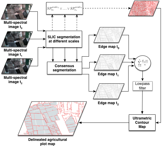
The methodology proposed in this paper integrates segmentation at different scales, carried out by an SP approach, and different dates to obtain a final single segmentation of the agricultural plots. An overview of the proposed methodology is shown in Figure 3.
The first step of this methodology is the image segmentation at different scales. Segmentation was carried out by means of the multispectral SLIC algorithm proposed in [30]. This method extends the original SLIC proposed in [31] by considering not only an RGB color space but a multispectral space. In this case, the clustering distance (Equation (1)) between two pixels and is composed of two components, one spatial () and the other spectral ().
where x and y denote the position of the pixels. B represents the total number of bands in the multispectral image. The constants g and c influence the size of the superpixel and its compactness, respectively. The higher the g value, the bigger the superpixel; on the other hand, the bigger the c value, the more compact the superpixel.
Segments at different scales are generated by fixing the value of the compactness parameter but varying the size of the SPs. Similar to [30], the number of SPs was selected to follow a dyadic progression. In this work, the three original images were segmented into 10 different scales using the SLIC algorithm. The parameters used in the segmentation are a compactness factor (c), which is 0.04 times the maximum spectral value contained in each of the image, and the number of SPs, which ranges from (scale) to (scale), on average.
The integration of the l segmentation for each date was carried out using a consensus process, which consists basically of a voting scheme that determines which pixels belong to the same region and which are part of the edges of objects in the image.
Thus, for each pair of adjacent pixels i and j, an value is obtained by Equations (4) and (5), which takes into account whether the pixels belong to the same region. If the two adjacent pixels (the ith and jth) do not belong to the same region, that means they are part of the edges between these regions. is defined as:
where and represent the regions a and b, respectively, belonging to the kth segmentation, and is an index of the similarity between the regions and . The larger the value of , the stronger the separation between these regions.
The similarity index, analogous to that proposed by [32], is defined as a combination between the similarity indices of color and texture:
where measures the color similarity. For each region , a color histogram is obtained using 25 bins for each spectral band. Then, from the color histograms, a feature vector with a length of is generated for region (u can be a and b), where B is the number of bands of the multispectral images. The feature vector is normalized using the norm (also known as the Manhattan norm). Finally, the color similarity between the two regions and is calculated using the statistic [33]:
where measures the texture similarity. Texture is calculated by means of steerable filters [34] using Gaussian derivatives in eight directions and as a basis. In this case, for each region , a texture histogram is obtained using 10 bins for each spectral band and each filter direction, resulting in 80 features. Then, from the texture histograms, a feature vector with a length is generated for each region , where B is the number of bands in the image. The similarity in texture between two regions and is calculated as follows:
The result of the consensus process is an edge map for each date that is generated with the information of the voting scheme, which is normalized to a range of 0–1. These maps combine different information, such as (i) different scales of segmentation through the different sizes of SPs, (ii) the dissimilarity in both texture and color between neighboring regions, and (iii) the probability of a pixel belonging to an edge. The closer to 1 the value of a pixel, the greater the probability of it belonging to an edge in the multiple segmentation scales, and, therefore, the contrast between regions separated by such a pixel at different scales is greater.
The next step in the methodology is the integration of the edge maps for all dates into the labeled boundaries (). In this work, this integration was carried out by averaging the n edge maps.
Low-pass filtering should be applied to reduce the noise present in . In this work, a median filter was used.
Since this averaged edge map generally includes open polygons, an ultrametric contour map (UCM) was calculated by means of the method proposed by [35]. A UCM is an edge map with the remarkable property, i.e., it produces a set of closed curves when any threshold is set [36]. The larger the threshold, the greater the contrast of the edges of the segments generated. The output of the UCM produces the outline of the final plots. In the end, a UCM is a soft representation of a segmentation that takes into account information from the edges of the image. The UCM has two inputs: the labeled boundaries (Equation (9)) and an image with boundary weights (IBW), which is defined by the Equation (10):
where and represent the SPs at scale 1 for the date and , respectively; and ∨ is the logical operator OR. A detailed description of the UCM algorithm can be found in [35].
3. Results and Discussion
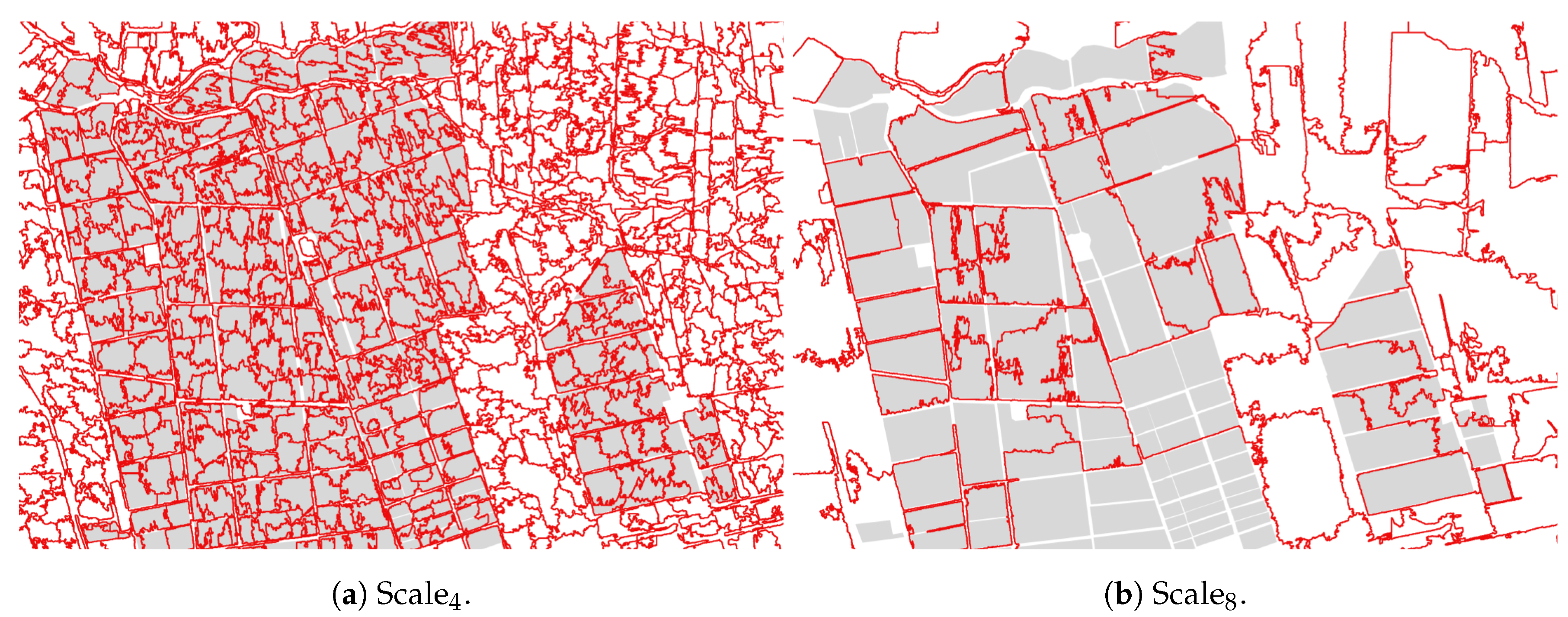
In Figure 4, the SP segmentation obtained for the image registered on 30 January 2018 and corresponding to scale and scale is overlaid onto the color-composition image. It is possible to see the good adherence of the SPs to image objects in the three displayed cases. However, it can also be observed that the smaller the SP size (Figure 4a), the better its adherence to the edges, as well as the homogeneity of the pixels that compose it. While, in the segmentation scales with larger SPs (Figure 4a,b), the segments are less spectrally homogeneous, they still respect the borders between regions with a high contrast (the thickest edges).
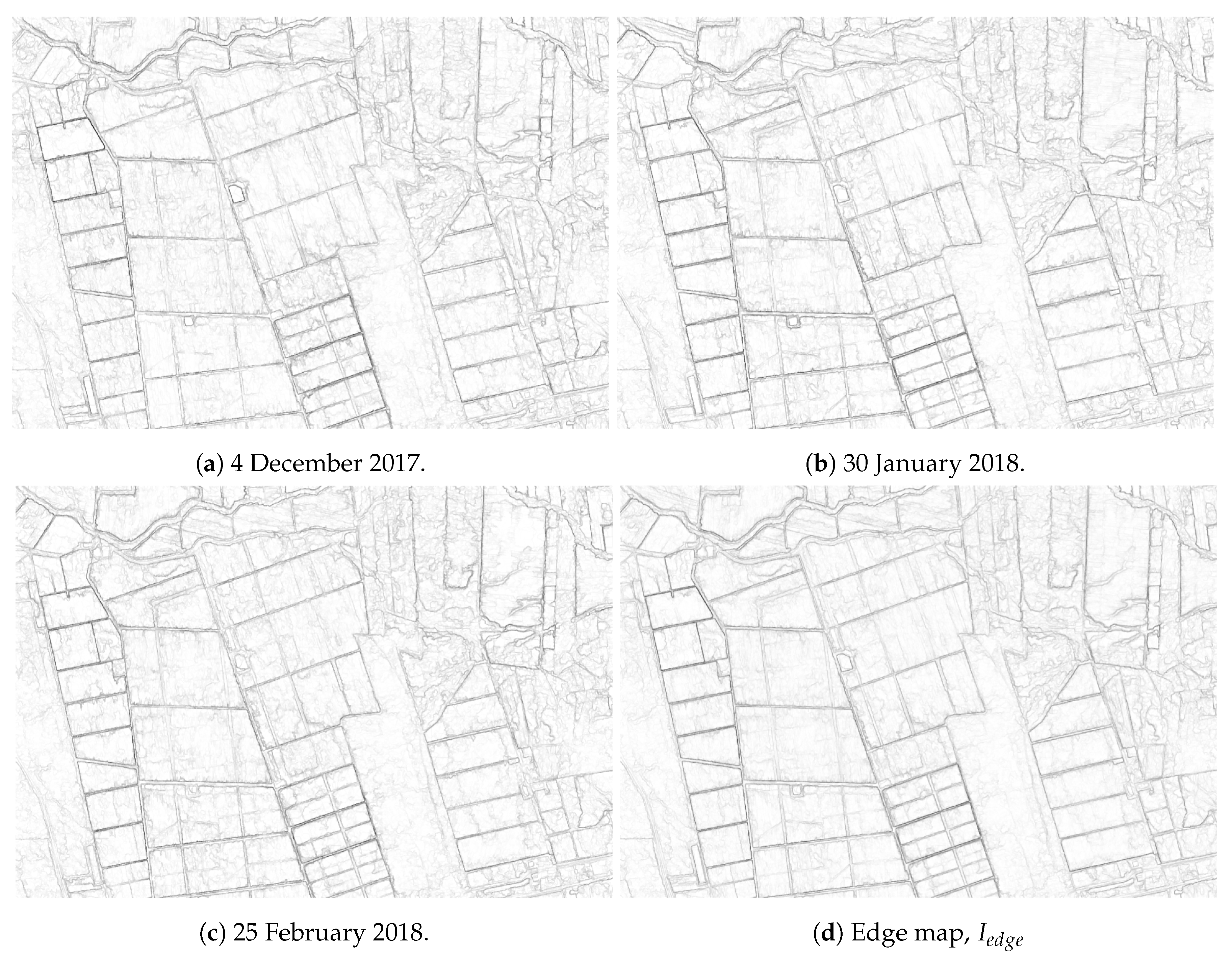
From the 10 segmentation scales for each date generated and consensus, the edge maps shown in Figure 5a–c were obtained.
As can be seen in Figure 5a–c, the edges of the plots tend to be more intense in all cases. In accordance with the methodology described, the next step is the integration of the three edge maps, one for each date, by calculating the average value. The average value is chosen as the basic form of integration because it allows for representing the information (borders) contained in all dates, thus reducing the effect of the appearance of borders in only one of the images, which is usually unusual for images of the same growing season (as mentioned in Section 1). In addition, the edges that appear as a result of phenological changes tend to decrease. The edge map obtained (Figure 5d) provides useful information for identifying the edges belonging to the plots; however, as mentioned above, it does not guarantee complete plots by applying a threshold, mainly due to edge-pixels not having the same value. Then, in order to obtain the final outlined agricultural plot map for the area considered, the UCM algorithm was applied to complete the edges.
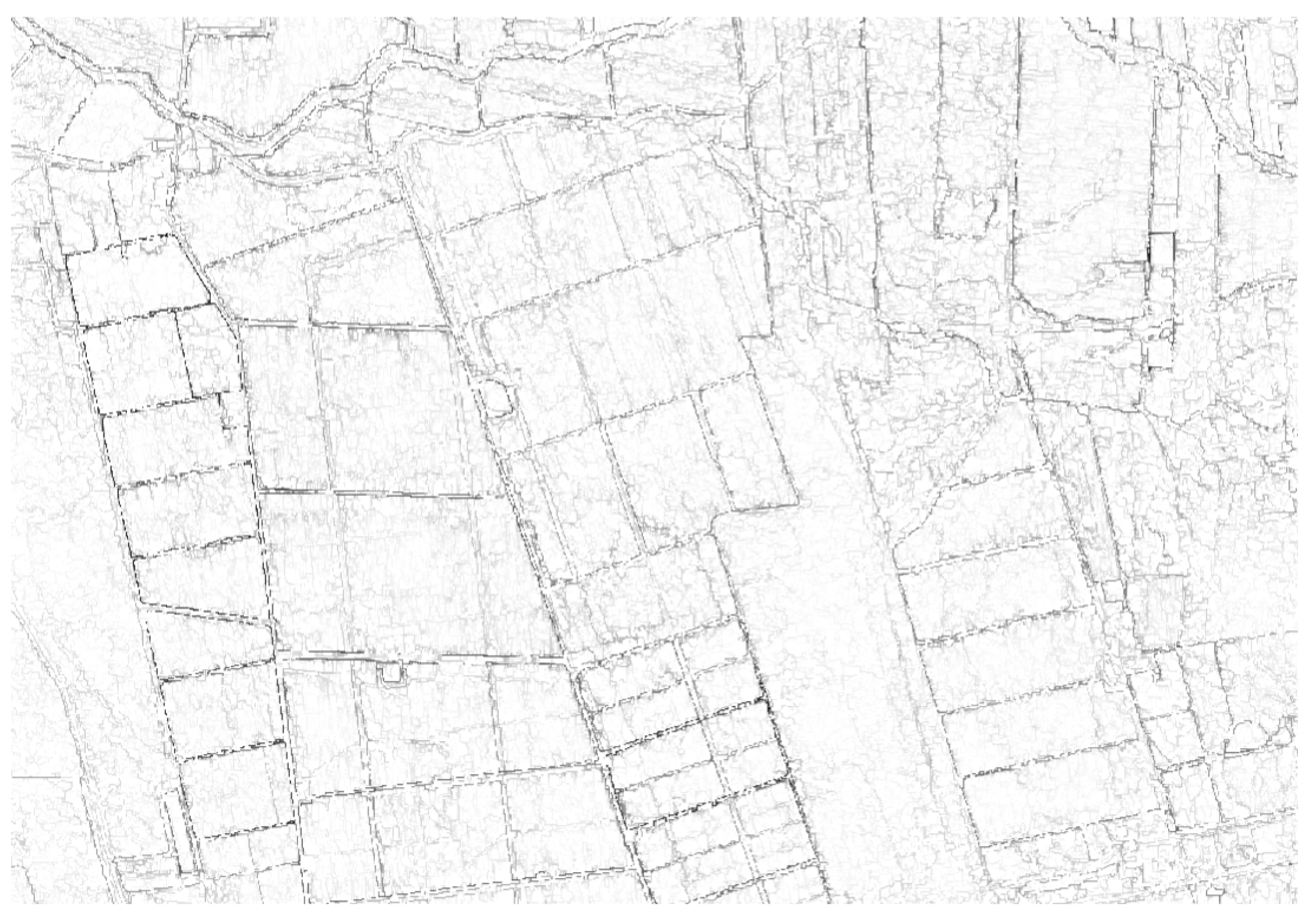
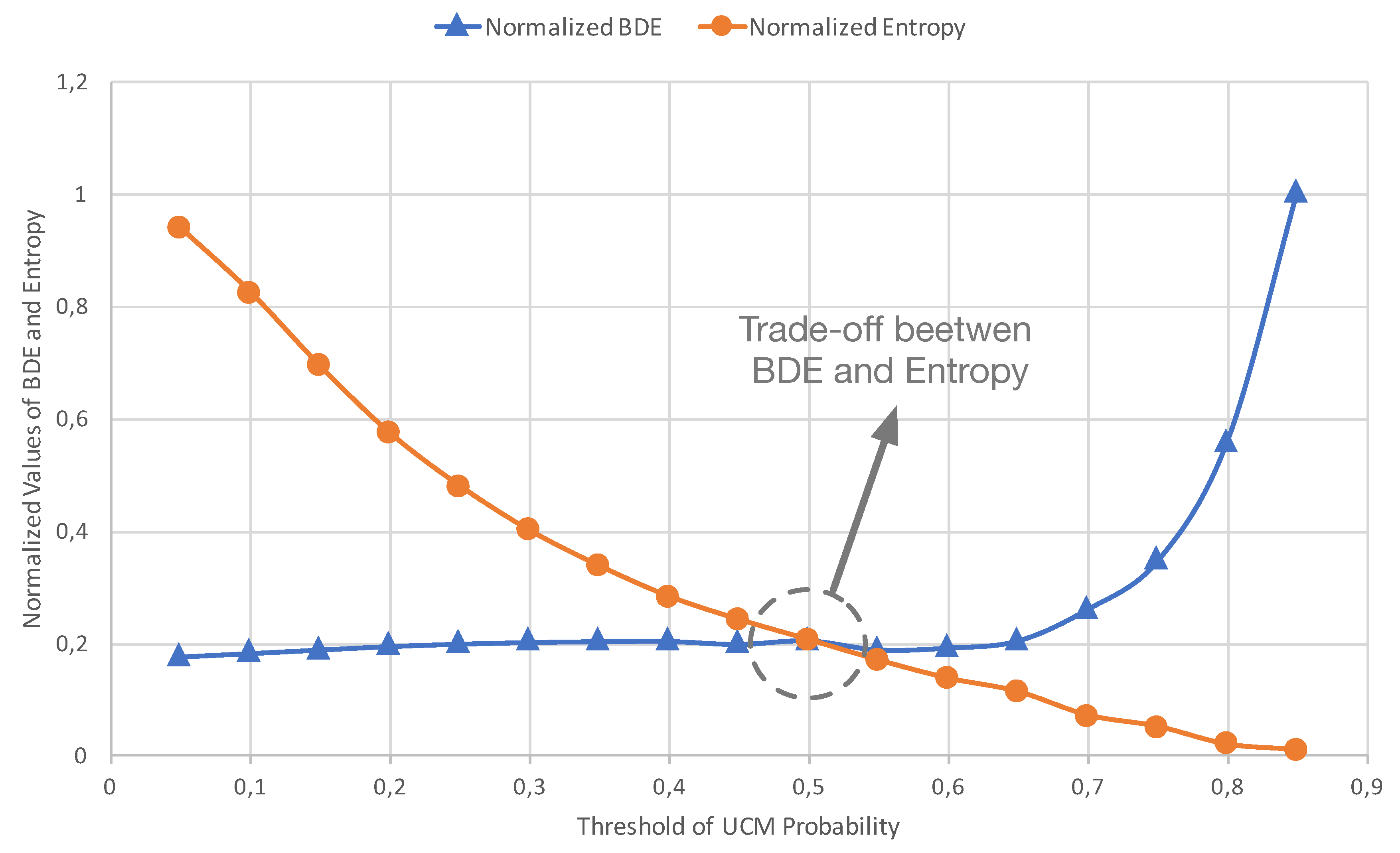
Figure 6 shows the result of applying the UCM algorithm to the average of the three edge maps (Figure 5d). As can be observed, even though all edges have been closed, there is a lot of noise inside each plot. This noise is due to the fact that in the UCM, the totality of the probabilities of occurrence of the edges is represented. This is why it is necessary to determine a threshold value of the probability above which an edge is considered as such. Two indicators were used to determine this value objectively. The first was an error metric of the calculated edges with respect to a ground truth called boundary displacement error (BDE) [37,38]; the second metric considers the Shannon entropy, which represents the information content present in a border image: in this case, it is the number of edges present at the UCM. The BDE index measures the difference between two segmented images by averaging the displacement of boundary pixels. Specifically, the distance () between a boundary pixel () in the obtained boundary image () and the closest pixel () in the ground-truth boundary image is used to define the error (disagreement) of each boundary pixel. The BDE index can be mathematically defined as in Equation (11).
where represents the number of boundary pixels in image B, and is the Euclidean distance. The BDE index ranges within , where the lower its value, the better. The BDE index is plotted against the edge entropy in Figure 5d for each threshold value. As shown in Figure 7, the smallest BDE metric error occurs for threshold values that are close to 1, while the worst values occur for values close to 0. Conversely, entropy behavior presents low values of information content for high threshold values and high information content for high threshold values. For the purpose of determining a specific threshold value, a compromise was established between the BDE value and the entropy value. As can be observed, a threshold value of 0.5 provides the balance between the error and the amount of edge information.
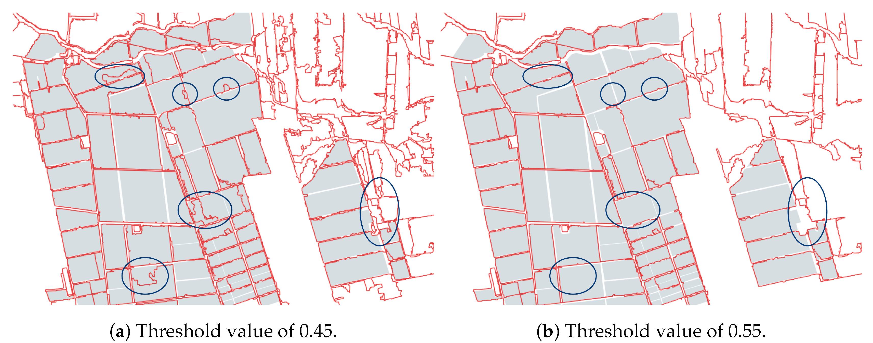
Figure 8 shows the final outlined plot maps obtained for two different threshold values overlaid onto the ground truth map.
As can be seen, most of the edges agree between the two maps (Figure 8a,b), particularly in homogeneous areas with a high contrast between adjacent regions; however, discrepancies in plots with different tilled patterns can be also distinguished where the appearance of inner edges is present, as in plots within which anomalies are perceived due to poor agricultural practices, land heterogeneity, or crop diseases. As an example of the above, some areas where these changes occur are shown enclosed in circles. Consequently, only the edges stable over time—those that appear in the two images—remain in the final outlined plot map.
4. Conclusions
In this work, a new methodology based on consensus segmentation for outlining agricultural plots is presented. The methodology proposed combines segmentation at different scales—carried out using an SP method—and images registered at different dates to obtain a single segmentation of the agricultural plots. This methodology allows the outlining of agricultural plots of different sizes, shapes, colors, and textures. It is based on a consensus of segmentation (SP) at different scales and for different dates to determine the boundaries of the agricultural plots. The segmentation at different scales allows different-sized plots to be outlined. The use of SP for segmentation, which shows a good adherence to the edges for all scales, allows for differently shaped plots to be outlined. By highlighting the stable edges over time, the consensus of the segmentation reduces the intra-plot variability caused by the phenological stages present in a single growing season. The methodology also allows a threshold value to be determined in an objective way, which establishes a balance between the error and the amount of edge information. In particular, in this study, the threshold value determined for balance was 0.5. For lower threshold values, edges that are less stable over time appear on the outlined plot map, while for threshold values of up 0.5, only the more stable edges over time appear on the map.
Author Contributions
For this research article, A.G.-P., C.G.-M., and M.L.-S. conceived of and designed the experiments. A.G.-P. carried out the experiments. A.G.-P., C.G.-M., and M.L.-S. analyzed the data and results and wrote the paper, and D.R.-E. checked the paper style.
Funding
This work has been partially funded by the Agencia Estatal de Investigación (AEI) of Spain and the European Regional Development Fund (ERDF) through the ARTeMISat-2 project: Advanced Processing of Remote Sensing Data for Monitoring and Sustainable Management of Marine and Terrestrial Resources in Vulnerable Ecosystems (CTM2016-77733-R), and by the Water Research Center For Agriculture and Mining, CRHIAM (CONICYT–FONDAP–1513001).
Acknowledgments
A.G.-P. thanks the support of the SEÑALES Project (VA026P17) financed by the Junta de Castilla y León and the European Regional Development Fund (ERDF).
Conflicts of Interest
The authors declare no conflict of interest.
Abbreviations
The following abbreviations are used in this manuscript:
| LPIS | Land Parcel Identification System |
| SLIC | Simple Linear Iterative Clustering |
| SP | Superpixels |
| UCM | Ultrametric Contour Map |
| VHSR | Very High Spatial Resolution |
References
- OECD/FAO. OECD-FAO Agricultural Outlook 2017–2026; Technical Report; OECD Publishing: Paris, France, 2017. [Google Scholar]
- Mirón Pérez, J. Cadastre and the Reform of European Union’s Common Agricultural Policy. Implementation of the SIGPAC. 2005. Available online: http://www.catastro.meh.es/documentos/publicaciones/ct/ct54/01-catastro54ing.pdf (accessed on 20 May 2017).
- Van Der Molen, P. The use of the Cadastre Among the Members States: Property Rights, Land Registration and Cadastre in the European Union. 2002. Available online: http://www.catastro.meh.es/documentos/publicaciones/ct/ct45/02ingles.pdf (accessed on 20 May 2017).
- Ciriza, R.; Sola, I.; Albizua, L.; Álvarez-Mozos, J.; González-Audícana, M. Automatic Detection of Uprooted Orchards Based on Orthophoto Texture Analysis. Remote Sens. 2017, 9, 492. [Google Scholar] [CrossRef]
- National Research Council. Need for a Multipurpose Cadastre; National Academy Press: Washington, DC, USA, 1980. [Google Scholar]
- National Research Council. National Land Parcel Data: A Vision for the Future; The National Academies Press: Washington, DC, USA, 2007. [Google Scholar]
- Leo, O.; Lemoine, G. Land Parcel Identification Systems in the Frame of Regulaton (EC) 1593/2000 Version 1.4; Technical Report; Institute for Environment and Sustainability: Ispra, Italy, 2001. [Google Scholar]
- Mulla, D.J. Twenty five years of remote sensing in precision agriculture: Key advances and remaining knowledge gaps. Biosyst. Eng. 2013, 114, 358–371. [Google Scholar] [CrossRef]
- Shelestov, A.Y.; Kravchenko, A.N.; Skakun, S.V.; Voloshin, S.V.; Kussul, N.N. Geospatial information system for agricultural monitoring. Cybern. Syst. Anal. 2013, 49, 124–132. [Google Scholar] [CrossRef]
- Waldner, F.; Canto, G.S.; Defourny, P. Automated annual cropland mapping using knowledge-based temporal features. ISPRS J. Photogramm. Remote Sens. 2015, 110, 1–13. [Google Scholar] [CrossRef]
- Khot, L.R.; Espinoza, C.Z.; Jarolmasjed, S.; Sathuvalli, V.R.; Vandemark, G.J.; Miklas, P.N.; Carter, A.H.; Pumphrey, M.O.; Knowles, N.R.; Pavek, M.J. Low-altitude, high-resolution aerial imaging systems for row and field crop phenotyping: A review. Eur. J. Agron. 2015, 70, 112–123. [Google Scholar]
- Mueller, M.; Segl, K.; Kaufmann, H. Edge- and region-based segmentation technique for the extraction of large, man-made objects in high-resolution satellite imagery. Pattern Recognit. 2004, 37, 1619–1628. [Google Scholar] [CrossRef]
- Da Costa, J.P.; Michelet, F.; Germain, C.; Lavialle, O.; Grenier, G. Delineation of vine parcels by segmentation of high resolution remote sensed images. Precis. Agric. 2007, 8, 95–110. [Google Scholar] [CrossRef]
- Tiwari, P.S.; Pande, H.; Kumar, M.; Dadhwal, V.K. Potential of IRS P-6 LISS IV for agriculture field boundary delineation. J. Appl. Remote Sens. 2009, 3, 033528. [Google Scholar] [CrossRef]
- Kass, M.; Witkin, A.; Terzopoulos, D. Snakes: Active contour models. Int. J. Comput. Vis. 1988, 1, 321–331. [Google Scholar] [CrossRef] [Green Version]
- Turker, M.; Kok, E.H. Field-based sub-boundary extraction from remote sensing imagery using perceptual grouping. ISPRS J. Photogramm. Remote Sens. 2013, 79, 106–121. [Google Scholar] [CrossRef]
- Garcia-Pedrero, A.; Gonzalo-Martin, C.; Fonseca-Luengo, D.; Lillo-Saavedra, M. A GEOBIA Methodology for Fragmented Agricultural Landscapes. Remote Sens. 2015, 7, 767–787. [Google Scholar] [CrossRef] [Green Version]
- Crommelinck, S.; Yang, M.Y.; Koeva, M.; Gerke, M.; Bennett, R.; Vosselman, G. Towards Automated Cadastral Boundary Delineation from UAV Data. arXiv, 2017; arXiv:1709.01813. [Google Scholar]
- García-Pedrero, A.; Gonzalo-Martín, C.; Lillo-Saavedra, M. A machine learning approach for agricultural parcel delineation through agglomerative segmentation. Int. J. Remote Sens. 2017, 38, 1809–1819. [Google Scholar] [CrossRef]
- Rodolà, E.; Bulò, S.R.; Cremers, D. Robust Region Detection via Consensus Segmentation of Deformable Shapes. Comput. Gr. Forum 2014, 33, 97–106. [Google Scholar] [CrossRef] [Green Version]
- Faktor, A.; Irani, M. Video Segmentation by Non-Local Consensus Voting. In Proceedings of the British Machine Vision Conference, Nottingham, UK, 1–5 September 2014; pp. 1–12. [Google Scholar]
- Carlier, T.; Haumont, C.; Bailly, C.; Bodet-Milin, C.; Ansquer, C.; Bodere, F. About few properties of PET segmentation using consensus approaches. J. Nucl. Med. 2017, 58, 611. [Google Scholar]
- Inglada, J.; Dejoux, J.F.; Hagolle, O.; Dedieu, G. Multi-temporal remote sensing image segmentation of croplands constrained by a topographical database. In Proceedings of the Geoscience and Remote Sensing Symposium (IGARSS), Munich, Germany, 22–27 July 2012; pp. 6781–6784. [Google Scholar]
- Blaes, X.; Vanhalle, L.; Defourny, P. Efficiency of crop identification based on optical and SAR image time series. Remote Sens. Environ. 2005, 96, 352–365. [Google Scholar] [CrossRef]
- Matton, N.; Canto, G.S.; Waldner, F.; Valero, S.; Morin, D.; Inglada, J.; Arias, M.; Bontemps, S.; Koetz, B.; Defourny, P. An Automated Method for Annual Cropland Mapping along the Season for Various Globally-Distributed Agrosystems Using High Spatial and Temporal Resolution Time Series. Remote Sens. 2015, 7, 13208–13232. [Google Scholar] [CrossRef] [Green Version]
- Kussul, N.; Lemoine, G.; Gallego, J.; Skakun, S.; Lavreniuk, M. Parcel Based Classification for Agricultural Mapping and Monitoring using Multi-temporal Satellite Image Sequences. In Proceedings of the Geoscience and Remote Sensing Symposium (IGARSS), Milan, Italy, 26–31 July 2015; pp. 165–168. [Google Scholar]
- Liu, Y.; Li, M.; Mao, L.; Xu, F.; Huang, S. Review of remotely sensed imagery classification patterns based on object-oriented image analysis. Chin. Geogr. Sci. 2006, 16, 282–288. [Google Scholar] [CrossRef]
- Huang, X.; Yang, W.; Xia, G.; Liao, M. Superpixel-based change detection in high resolution SAR images using region covariance features. In Proceedings of the 2015 8th International Workshop on the Analysis of Multitemporal Remote Sensing Images (Multi-Temp), Annecy, France, 22–24 July 2015; pp. 1–4. [Google Scholar]
- Wu, Z.; Hu, Z.; Fan, Q. Superpixel-based unsupervised change detection using multi-dimensional change vector analysis and SVM-based classification. ISPRS Ann. Photogramm. Remote Sens. Spat. Inf. Sci. 2012, 7, 257–262. [Google Scholar] [CrossRef]
- Gonzalo-Martín, C.; Lillo-Saavedra, M.; Menasalvas, E.; Fonseca-Luengo, D.; García-Pedrero, A.; Costumero, R. Local optimal scale in a hierarchical segmentation method for satellite images. J. Intell. Inf. Syst. 2016, 46, 517–529. [Google Scholar] [CrossRef]
- Achanta, R.; Shaji, A.; Smith, K.; Lucchi, A.; Fua, P.; Süsstrunk, S. SLIC superpixels compared to state-of-the-art superpixel methods. IEEE Trans. Pattern Anal. Mach. Intell. 2012, 34, 2274–2282. [Google Scholar] [CrossRef] [PubMed]
- Uijlings, J.R.; van de Sande, K.E.; Gevers, T.; Smeulders, A.W. Selective search for object recognition. Int. J. Comput. Vis. 2013, 104, 154–171. [Google Scholar] [CrossRef]
- Rubner, Y.; Tomasi, C.; Guibas, L.J. The earth mover’s distance as a metric for image retrieval. Int. J. Comput. Vis. 2000, 40, 99–121. [Google Scholar] [CrossRef]
- Freeman, W.T.; Adelson, E.H. The design and use of steerable filters. IEEE Trans. Pattern Anal. Mach. Intell. 1991, 13, 891–906. [Google Scholar] [CrossRef] [Green Version]
- Arbelaez, P.; Maire, M.; Fowlkes, C.; Malik, J. From contours to regions: An empirical evaluation. In Proceedings of the IEEE Conference on Computer Vision and Pattern Recognition CVPR 2009, Miami Beach, FL, USA, 20–25 June 2009; pp. 2294–2301. [Google Scholar]
- Dollár, P.; Zitnick, C.L. Structured forests for fast edge detection. In Proceedings of the IEEE International Conference on Computer Vision, Sydney, Australia, 1–8 December 2013; pp. 1841–1848. [Google Scholar]
- Freixenet, J.; Muñoz, X.; Raba, D.; Marti, J.; Cufí, X. Yet another survey on image segmentation: Region and boundary information integration. In European Conference on Computer Vision; Springer: Berlin/Heidelberg, Germany, 2002; pp. 408–422. [Google Scholar]
- Yang, A.Y.; Wright, J.; Ma, Y.; Sastry, S.S. Unsupervised segmentation of natural images via lossy data compression. Comput. Vis. Image Underst. 2008, 110, 212–225. [Google Scholar] [CrossRef] [Green Version]
Figure 1.
Study site, located in the Lolol Valley, O’Higgins Region, Chile.

Figure 2.
Color compositions (3-2-1) of the Plèiades-1 imagery for three different dates and the ground truth of the study area.
Figure 2.
Color compositions (3-2-1) of the Plèiades-1 imagery for three different dates and the ground truth of the study area.

| 0.48 | 0.48 |
| (a) b | (b) b |
| 0.48 | 0.48 |
| (c) b | (d) b |
Figure 3.
Overview of the methodology proposed.

Figure 4.
Superpixels for different scales are overlaid onto the ground truth of the study area with red color.
Figure 4.
Superpixels for different scales are overlaid onto the ground truth of the study area with red color.

| 0.48 | 0.48 |
| (a) b | (b) b |
Figure 5.
Edge maps for three dates and the edge map, , obtained by averaging the three dates’ edge maps.
Figure 5.
Edge maps for three dates and the edge map, , obtained by averaging the three dates’ edge maps.

| 0.48 | 0.48 |
| (a) b | (b) b |
| 0.48 | 0.48 |
| (c) b | (d) b |
Figure 6.
Result of applying the ultrametric contour map (UCM) algorithm to the average of the three edge-maps.
Figure 6.
Result of applying the ultrametric contour map (UCM) algorithm to the average of the three edge-maps.

Figure 7.
Representation of error versus the edge entropy for different threshold values.

Figure 8.
Final outlined plot maps obtained for two different threshold values.

| 0.45 | 0.45 |
| (a) b | (b) b |

Table 1.
Spectral and spatial characteristics of the multispectral image taken by the Plèiades-1 satellite.
Table 1.
Spectral and spatial characteristics of the multispectral image taken by the Plèiades-1 satellite.
| Band Name | Bandwidth (nm) | Spatial Resolution (m) |
|---|---|---|
| blue | 430–550 | 2 |
| green | 490–610 | |
| red | 600–720 | |
| near infrared | 750–950 |
© 2018 by the authors. Licensee MDPI, Basel, Switzerland. This article is an open access article distributed under the terms and conditions of the Creative Commons Attribution (CC BY) license (http://creativecommons.org/licenses/by/4.0/).
Share and Cite
MDPI and ACS Style
Garcia-Pedrero, A.; Gonzalo-Martín, C.; Lillo-Saavedra, M.; Rodríguez-Esparragón, D. The Outlining of Agricultural Plots Based on Spatiotemporal Consensus Segmentation. Remote Sens. 2018, 10, 1991. https://doi.org/10.3390/rs10121991
AMA Style
Garcia-Pedrero A, Gonzalo-Martín C, Lillo-Saavedra M, Rodríguez-Esparragón D. The Outlining of Agricultural Plots Based on Spatiotemporal Consensus Segmentation. Remote Sensing. 2018; 10(12):1991. https://doi.org/10.3390/rs10121991
Chicago/Turabian StyleGarcia-Pedrero, Angel, Consuelo Gonzalo-Martín, Mario Lillo-Saavedra, and Dionisio Rodríguez-Esparragón. 2018. "The Outlining of Agricultural Plots Based on Spatiotemporal Consensus Segmentation" Remote Sensing 10, no. 12: 1991. https://doi.org/10.3390/rs10121991
Note that from the first issue of 2016, this journal uses article numbers instead of page numbers. See further details here.