Two-Step Urban Water Index (TSUWI): A New Technique for High-Resolution Mapping of Urban Surface Water

1
Institute of Remote Sensing and Digital Earth, Chinese Academy of Sciences, No. 20 Datun Road, Chaoyang District, Beijing 100101, China
2
University of Chinese Academy of Sciences, Beijing 100049, China
*
Authors to whom correspondence should be addressed.
Remote Sens. 2018, 10(11), 1704; https://doi.org/10.3390/rs10111704
Submission received: 19 September 2018
/
Revised: 16 October 2018
/
Accepted: 26 October 2018
/
Published: 29 October 2018
(This article belongs to the Special Issue Very High Resolution (VHR) Satellite Imagery: Processing and Applications)
Abstract
:Urban surface water mapping is essential for studying its role in urban ecosystems and local microclimates. However, fast and accurate extraction of urban water remains a great challenge due to the limitations of conventional water indexes and the presence of shadows. Therefore, we proposed a new urban water mapping technique named the Two-Step Urban Water Index (TSUWI), which combines an Urban Water Index (UWI) and an Urban Shadow Index (USI). These two subindexes were established based on spectral analysis and linear Support Vector Machine (SVM) training of pure pixels from eight training sites across China. The performance of the TSUWI was compared with that of the Normalized Difference Water Index (NDWI), High Resolution Water Index (HRWI) and SVM classifier at twelve test sites. The results showed that this method consistently achieved good performance with a mean Kappa Coefficient (KC) of 0.97 and a mean total error (TE) of 5.82%. Overall, classification accuracy of TSUWI was significantly higher than that of the NDWI, HRWI, and SVM (p-value < 0.01). At most test sites, TSUWI improved accuracy by decreasing the TEs by more than 45% compared to NDWI and HRWI, and by more than 15% compared to SVM. In addition, both UWI and USI were shown to have more stable optimal thresholds that are close to 0 and maintain better performance near their optimum thresholds. Therefore, TSUWI can be used as a simple yet robust method for urban water mapping with high accuracy.
1. Introduction
Urban surface water such as rivers, lakes, reservoirs, and ponds, exerts a significant influence on urban ecosystem services [1] and local microclimates [2]. As a consequence of Land Use/Land Cover (LULC) and environmental changes and natural hazards, variations in urban surface water, may result in a series of ecological, climate, health, and socioeconomic problems, such as water supply shortages [3,4], biodiversity losses [5], aggravation of the urban heat island effect [6,7], and even outbreaks of waterborne infectious diseases [8]. These problems tend to be more prominent in cities with rapid urbanization [9,10,11,12]. With the development of urbanization, the urban space has been expanded, leading to the shrinking of water bodies. Meanwhile, frequent human activities may lead to the deterioration of water quality towards being turbid, stink, or black. Therefore, timely and accurate mapping of urban surface water is crucial for urban planning and disaster assessments [13,14].
Remote sensing techniques, with their advantages of large area coverage, integration, speed, and periodicity, have been widely used to delineate surface water and monitor surface water dynamics. Various methods have been proposed to identify surface water bodies, which can be divided into four types: thematic classification [15,16], spectral unmixing [17,18,19], single band thresholding [20,21], and spectral water index [22,23,24]. The last is the most widely used, due to its ease of use, relatively high mapping accuracy, and low computational expense [25]. Over the past few decades, many water indexes have been presented in the literature. McFeeters [23] proposed the first water index called the Normalized Difference Water Index (NDWI) with a default threshold of 0, which utilized the reflectance difference between water and vegetation and soil in the red and near-infrared (NIR) bands. To suppress the signals from buildings, Xu [24] replaced the NIR band with the shortwave infrared (SWIR) band in the NDWI formulation, creating the Modified Normalized Difference Water Index (MNDWI). Although the MNDWI shows high accuracy, it was still unable to suppress shadows. Therefore, Feyisa et al. [22] proposed an automated water extraction index (AWEI) and that has been demonstrated to be effective in different environments, particularly in mountainous areas with deep shadows.
However, mapping small and narrow urban surface water bodies requires the adoption of high-resolution images [26]. Most high-resolution images, such as Gaofen-2 (GF-2), IKONOS, RapidEye and Ziyuan-3 (ZY-3), have only visible and NIR bands and lack the bands necessary to compute most of the conventional water indexes designed for low- or medium-resolution images. This condition necessitates the development of a water index for fast and accurate mapping of urban surface water. Compared to water detection in rural areas, the complex urban setting poses great challenges for mapping water bodies with high-resolution imagery. Because urban water is greatly affected by human activities, it may contain high amounts of pollutants, such as suspended solids, high levels of nutrients, heavy metals, and sewage runoff. These pollutants make the spectral properties of urban surface water quite different from those of unpolluted water [27]. In addition, abundant shadows cast by tall buildings and trees are present in remotely sensed images in urban areas. Due to the similarity in spectral patterns between shadows and water, it is difficult to remove shadow noise from urban water maps.
NDWI and High Resolution Water Index (HRWI) are two water indexes commonly used for urban water extraction. However, NDWI tends to misclassify buildings and shadows as water when applied to high-resolution images [28]. HRWI is a water index that was proposed by Yao et al. [29]. HRWI also exhibits limited ability to distinguish shadows and should be applied together with a shadow detection model. Summaries of the aforementioned water indexes are presented in Table S1. To the best of our knowledge, a water index for high-resolution images with four standard bands that can effectively suppress all non-water pixels and extract urban water with high accuracy has not been proposed.
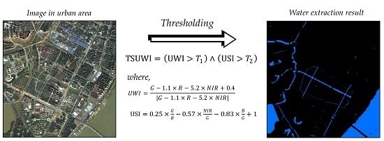
In this paper, a new urban water index, called the Two-Step Urban Water Index (TSUWI), was proposed to map urban water bodies from high-resolution imagery based on the full utilization of the spectral information from different objects in the visible and NIR bands. As one simple water index may not address all issues at the same time, the TSUWI combines two subindexes of an urban water index (UWI) and an urban shadow index (USI). The TSUWI proposed in this paper is expected to improve the accuracy of urban water mapping by suppressing the signal from artificial construction and shadows, and to be robust under various water conditions with stable thresholds and high accuracy.
2. Study Areas and Materials
2.1. Study Sites
Given the complex terrain and distinct climates over China, a total of twelve study sites with variable environmental conditions and diverse types of water bodies were selected to establish and validate the new urban water index. According to different application goals, these study sites were divided into two types: training sites and test sites.
Training sites were used for pure pixel selection to formulate the new urban water extraction index. Given that the features of urban surfaces are spatially variant, eight training sites characterized by different surface water types, climates, topographies, and urban development levels were therefore deliberately chosen. The sites were selected from eight cities around China: Chengdu, Guangzhou, Nanchang, Qingdao, Shanghai, Aksu, Lhasa and Shigatse (Figure 1). While covering all major challenging issues affecting the accuracy of urban water extraction, such as shadows, low-albedo buildings and black soil, these sites span across water bodies of different depths, turbidity levels, chemical compositions, and surface appearances, including rivers, lakes, reservoirs, pools and seas. The sites in Chengdu, Guangzhou, Nanchang, Qingdao and Shanghai are located in eastern China within a dense water network. The water bodies in Chengdu, Guangzhou, and Nanchang are typical inland waters and consist of several main rivers surrounded by many small ponds, regular or irregular lakes and artificial reservoirs. The main rivers in Chengdu are relatively narrow, while those in Nanchang are turbid with large amounts of fluid mud. Qingdao and Shanghai are coastal port cities containing both marine and inland water bodies. The site in Qingdao has harbors, tidal creeks, and a portion of the sea, and the main water body in Shanghai is a complicated mixture of suspended sediment and intrusive seawater because of its special location in the turbidity maximum zone of the Yangtze River Estuary. Aksu, Lhasa and Shigatse were selected to represent water bodies in China’s western cities, which tend to be rare and shallow due to the arid or semiarid climates. The site in Aksu primarily has a narrow river and a large shallow lake. Both sites in Lhasa and Shigatse have a narrow river, but part of the river in Shigatse is semi-dry.
Test sites were selected to assess the accuracy and robustness of the TSUWI. The whole image at each test site were used to delineate the true water body boundaries for the assessments. Considering that the pure pixels sampled for the development of the TSUWI covered only an extremely small portion of the image, the aforementioned eight training sites were also used as test sites. To enhance the reliability of the assessments, another four test sites located in Fuzhou, Haerbin, Yinchuan, and Dongguan were added to constitute the set of test sites. Fuzhou, Haerbin, and Dongguan are located in Eastern China where there are plenty of water bodies, while Yinchuan is located in Western China where water bodies are scarce. These twelve test sites are distributed across different regions of China (Figure 1). The wide range of variability in water types and environmental conditions of the twelve test sites imposes great difficulty for accurately mapping urban water bodies, which makes these sites ideal test sites. Table 1 shows the detailed descriptions of these twelve study sites.
2.2. GF-2 Imagery
As a civil land observation satellite with currently the highest resolution in China, GF-2 is equipped with two multispectral scanners and characterized by submeter spatial resolution, high positioning accuracy and rapid posture maneuverability. With a revisit cycle of 5 days and a swath width of 45 km, GF-2 is a critical data source for urban remote sensing applications. The basic characteristics of GF-2 satellite is shown in Table 2.
Twelve GF-2 images were ordered from the website of the China Center for Resources Satellite Data and Application (available at http://cresda.com/CN/index.shtml). One image was used for each site. When choosing images, all available data were inspected to avoid the influence of clouds on the water bodies. The GF-2 images contain one panchromatic band and four multispectral bands (comprised of blue, green, red, and near-infrared bands). All images were Level 1A products, which contain enough information for further image preprocessing, such as radiometric correction and geometric correction. The detailed information on these GF-2 images is presented in Table 3.
2.3. Reference Data
The true water body boundaries of all twelve study sites were manually digitized on-screen to evaluate the accuracies of the extracted water surface. In consideration of the inevitable bias caused by the time span between GF-2 images and other data sources, the digitization was implemented on the GF-2 images, which was sharpened by the panchromatic band with higher spatial resolution. Water conditions are sometimes extremely complicated, and small urban water bodies adjacent to tall buildings, especially dark and quadrangle-shaped buildings, could easily be confused with building shadows due to their similar spectra and morphology. Google EarthTM images, which were acquired on dates as close as possible to the GF-2 images, were supplied to assist with the visual interpretation by providing another different overview of the urban surfaces. Table 3 lists the detailed information about these supplementary reference data.
2.4. Image Preprocessing
The GF-2 images in the form of raw digital number (DN) values were calibrated to the top of atmosphere (TOA) reflectance via radiometric calibration. Atmosphere scattering and absorption could bring unexpected spectral bias, leading to significantly reduced image quality. As a consequence, an atmospheric correction was applied to the obtained TOA reflectance using the Fast Line-of-Sight Atmospheric Analysis of Spectral Hypercubes (FLAASH) module in ENVI v.5.3 [30]. Relative atmospheric parameters were determined via a lookup table [31], which is based on a seasonal-latitude surface temperature model. The initial visibility applied in this procedure was estimated using the aerosol optical depth (AOD) obtained from MODIS Terra aerosol products of version 6 [22].
Due to the effects of sensor tilt and terrain relief, orthorectification was carefully undertaken with the GF-2 images after atmospheric correction. Given that each GF-2 image contains Rational Polynomial Coefficient (RPC) information in the header file, this procedure was performed using the RPC orthorectification workflow in ENVI v5.3. To improve the precision of the geometric correction, ground control points (GPCs) with average root mean square (RMS) values of no more than 0.5 pixels were selected for each image to refine the RPCs, and the high-resolution digital elevation data (30 m) of ASTER GDEM v.2 [32] were supplied. The output pixel sizes for panchromatic band and multispectral bands are 1 m and 4 m, respectively. Afterwards, all orthorectified images were clipped to achieve higher urban water percentages and lower visual interpretation costs.
3. Methodology
3.1. Pure Pixel Selection
A dataset of pure pixel reflectance values of nine major urban land cover types was sampled from the GF-2 multispectral images of eight training sites. The urban land cover types are bright soil, black soil, bright built, dark built, vegetation, asphalt, light shadow, dark shadow, and water. These pure pixels were utilized to examine the spectral differences between water and other land cover types and act as samples fed into a linear Support Vector Machine (SVM) model for index coefficient training, aiming to design an urban water index that accurately distinguishes water from other urban surfaces. This new index is expected to be robust against various water type changes within complex urban environments. Therefore, as discussed in Section 2.1, eight training sites located in different cities across China, including a wide range of water types and all the major interference factors, were used to extract pure pixels.
Pure pixels were generated by manual digitization of the GF-2 multispectral images with the assistance of Google EarthTM images. Pure pixels were generally extracted from the center of a land cover patch to ensure their purity and were evenly distributed across each image to achieve high representativeness. For each of the eight training sites, 120 pixels were extracted for each land cover type, leading to 1080 pure pixels for each training site and 8640 for all sites.
3.2. Spectral Features of Water and Non-Water Types
Water indexes are typically mathematic combinations of several spectral features, aiming to enhance the contrast between water and non-water pixels [22]. Given the distinct separability of each feature for various land cover types, an optimal feature combination is required for an effective water index. Therefore, comprehensive analyses of the spectral characteristics of water and other land cover types are prerequisites for identifying the optimal feature combination to be applied in the formulation. Statistical distributions of pure pixel reflectance values of nine land cover types for blue, green, red, and NIR bands were obtained and displayed in Figure 2a–d. The results showed that the original bands generally demonstrated good performance in discriminating water from non-water types. However, considerable spectral overlap can be observed between water and dark shadows in all bands, making it difficult to extract water information while suppressing the shadow noise. To account for this issue, the TSUWI was proposed, which consisted of two subindexes of UWI and USI derived from different feature combinations. The UWI is formulated to effectively discriminate water and dark shadows from other non-water types, and the USI is formulated to remove the dark shadow pixels included in the extraction result of the UWI.
For the UWI, the optimal feature combination was identified from the image bands. Figure 2a–d showed that each band has a certain ability to separate water and dark shadows from other land cover types, and the red band achieves the best separability. However, the unstable reflectance values in the blue band may cause obvious variations in the optimal threshold values of the index [29], and no significant improvement in accuracy was observed after the blue band was introduced (discussed in Section 3.3.2). Therefore, the green, red and NIR bands were finally selected to formulate the UWI.
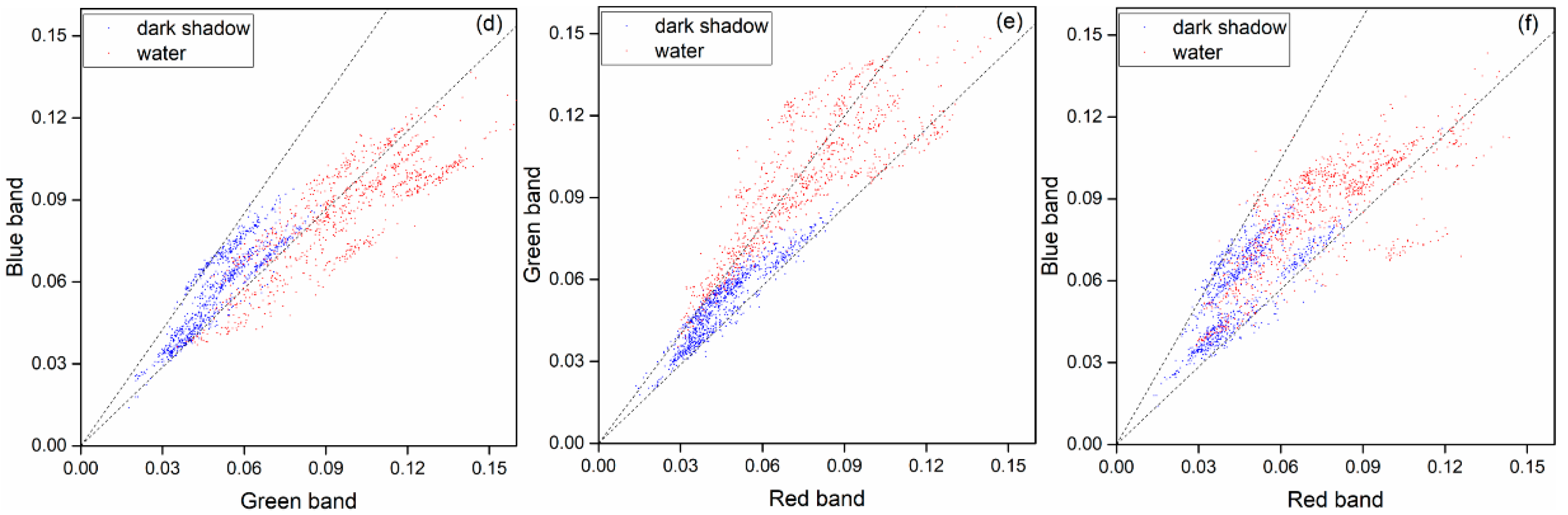
Band ratios were found to be capable of amplifying the minor differences between the spectral reflectance of water and dark shadows. Meanwhile, band ratios can also help stabilize the discrimination abilities of indexes by diminishing the undesired influence posed by topographic relief and light intensity change. Hence, six band ratios composed of either two of all four bands were calculated for the identification of the optimal feature combination for USI formulation, including NIR/B, NIR/G, NIR/R, B/G, B/R, and G/R, where G, R, B, and NIR refer to the reflectance values of the green, red, blue, and near infrared bands, respectively. Information redundancy exists among the six band ratios, and only three of them can cover all four bands. The three band ratios with maximum separability and minimum correlation were then chosen to formulate the USI. Scatter plots and M-statistical tests were used to qualitatively and quantitatively measure the separability of water and dark shadows in the band ratios. In the scatter plots shown in Figure 3, the area encompassed by the two dashed lines in each plot shows the locations of pure dark shadow pixels in the corresponding band ratio. Therefore, the more pure water pixels that fell out of this area, the better separability the band ratio has. The M-statistical test (Equation (1)) is defined by quantifying the histogram difference between two classes [33]. M values above 1.0 indicate fine separation, while M values below 1.0 indicate poor separation.
where is the difference in the means of two classes, and is the sum of their standard deviations. Considering that the USI is a linear combination of features, Pearson’s Correlation Coefficient (PCC) analysis [34] was used to examine the linear correlation between two band ratios. The closer a correlation coefficient to 1 or −1 is, the more significant the linear relation is, indicating that one band ratio is more likely to be superseded by the other.
Separability results revealed that NIR/G, NIR/B, and NIR/R showed similar scattering distribution patterns (Figure 3), and NIR/G achieved the best performance at separating water and dark shadows with a high M value of 1.12 (Table 4). The PCC analysis further confirmed that there are high correlations among NIR/G, NIR/B, and NIR/R, with correlation coefficients greater than 0.91. Hence, NIR/G was chosen, while both NIR/B and NIR/R were discarded. The other three band ratios of B/G, G/R, and B/R have M values of 0.91, 0.57, and 0.24, respectively. B/G and B/R are highly correlated with a coefficient of 0.71, while G/R and B/G are only weakly correlated with a coefficient of −0.25 (Table 5). Consequently, B/G and G/R were selected as the other two band ratios used in the formulation of the USI. Any two of the selected band ratios (NIR/G, B/G and G/R) were significantly correlated (Table 5).
3.3. Constructing the Two-Step Urban Water Index
The TSUWI was devised to effectively suppress non-water surfaces and extract urban water with improved accuracy. As discussed in Section 3.2, the spectral features used to eliminate water dark shadows differ from those used for other non-water types. Therefore, the TSUWI was designed to compose the two subindexes of the UWI and USI, the coefficients of which were obtained using linear SVM.
3.3.1. Linear Support Vector Machine
The coefficients of the water indexes imply the contribution of a corresponding feature to the separation of water and non-water pixels and become a significant issue for the design of a water index. The coefficients of conventional water indexes (e.g., NDWI, MNDWI, and AWEI) primarily resulted from reflectance pattern analysis of various land cover types, and therefore are characterized by certain subjectivity. In addition, because urban water bodies are typically sediment-rich and algae polluted and exhibit complicated optical features [35], it would become a great challenge for index designers to empirically determine the coefficients of an effective urban water index. In this paper, creating a new index is essentially a linear problem. Hence, the linear SVM was adopted to identify the optical coefficients for the new water indexes.
Linear SVM is a nonparametric statistical learning machine based on the structural risk minimization criterion [36]. By recovering an optical linear hyperplane in the feature space that maximizes the margin separation of two classes, it has been proven to be an advanced coefficient training model [29]. Given a set of labeled training data (X, Y) = {(xi, yi)|i = 1, …, N, yi ∈ {−1,1}}, the margin of the positive class is represented by equation 1, while the margin of the negative class is represented by equation −1. That is to say, the minimum margin difference between these two classes is 2, which ensures that the classifier has stable discrimination ability. The linear SVM can be explicitly formulated by solving the following constrained optimization problem (Equations (2) and (3)) [37].
where is the feature vector of training sample i, here referring to the optimal feature combination selected for index formulation. is the corresponding class label. N is the total number of training samples. is the Lagrangian multiplier ranging from 0 to a constant C. Weight vector w is a normal vector that is perpendicular to the hyperplane, and parameter b stands for the intercept term of the hyperplane.
The optical hyperplane is then represented by Equation (4).
For a test pixel x, if the expression output is greater than 0, it belongs to the positive class, and if the expression output is less than 0, it belongs to the negative class. Obviously, the expression can be used as an index, and parameters are the coefficients. In addition to enhancing the separability of the positive and negative classes, the linear SVM also provided a default threshold of 0, which could be used as a reasonable starting threshold for binary classification.
3.3.2. Formulation of the Urban Water Index (UWI)
The UWI was formulated using the linear SVM to discriminate water and dark shadows from other land cover types. Pure pixels of all land cover types were used to train the linear SVM, where water and dark shadow pixels are labeled as 1, and the other pixels are labeled as −1. To help determine whether the blue band should be introduced into the new index, two linear SVM training experiments were conducted with and without the blue band. By comparing their classification abilities using pure pixels, it was found that the addition of the blue band led to a reduced accuracy of 94.14% compared with 94.27%. The feature combination composed of the green, red, and NIR bands was thus used as the input training vector. After training, the coefficients for the optimal hyperplane were obtained (Equation (5)).
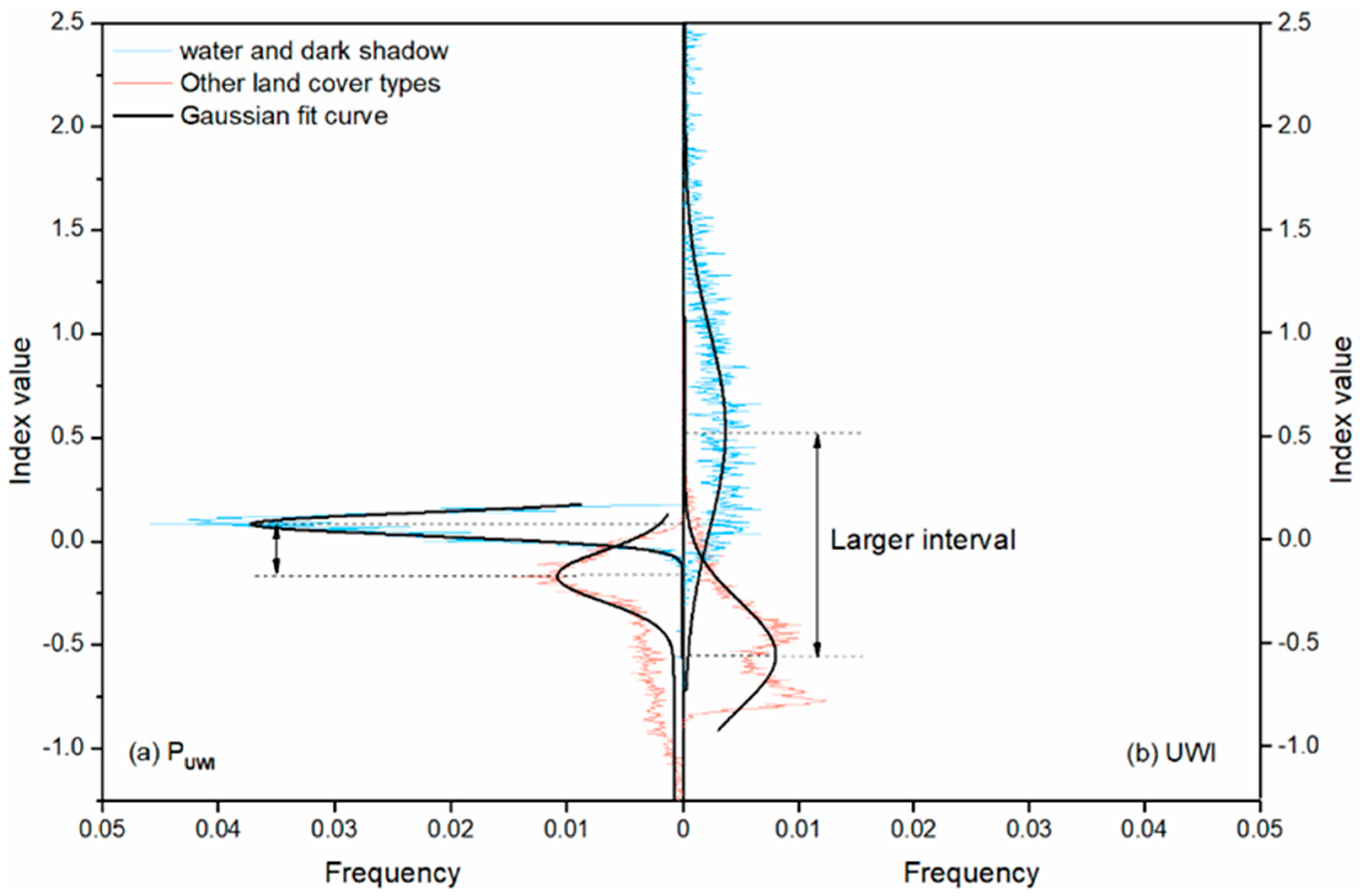
As shown in Figure 4a, the PUWI values of water and dark shadows did not display great discrepancy with the values of other land cover types. To further enhance the separation ability, PUWI was then divided by the expression |5.83 × G − 6.57 × R − 30.32 × NIR| to create the UWI. This division enlarged the difference that water and dark shadows had from other types. Providing insights into the histogram of pure pixel samples, it functioned by shifting water and dark shadow pixels towards larger positive values and shifting other land cover pixels towards smaller negative values, leading to a larger interval between them (Figure 4a,b). The modulus keeps the plus-minus sign unchanged, which means the water and dark shadow pixels in the UWI remain above 0 and other non-water pixels remain below 0. For ease of use, the common divisor 5.83 was removed in the final index, and the coefficients were rounded to one decimal digit, which did not cause a significant reduction in accuracy. The UWI formula is then represented by Equation (6).
3.3.3. Formulation of the Urban Shadow Index (USI)
The USI was designed to further improve the accuracy by removing the dark shadows that can be confused with water classes from the extraction result of the UWI. Herein, pure water and dark shadow pixels with NIR/G, B/G and G/R features were fed into the linear SVM to create the new USI. Pure water pixels were labeled as 1, and pure dark shadow pixels were labeled as −1. For ease of use, the coefficients of band ratios were rounded to two decimal digits, while one decimal digit was reserved in the constant term. The USI was finally formulated as shown in Equation (7).
3.3.4. The Two-Step Urban Water Index
The TSUWI was developed by combining the UWI and USI. The TSUWI extracts urban water by sequentially applying the UWI and USI to the image. The UWI was first applied to generate a temporary water mask. The USI was then used to eliminate dark and light shadow pixels included in the temporary water mask and obtain the final water extraction result. Therefore, the TSUWI can then be expressed as Equation (8).
Here, the TSUWI is a binary index with its possible values being 0 or 1. A value of 0 indicates non-water, while 1 indicates water. T1 and T2 denote the optimal thresholds of the UWI and USI, respectively. Zero could theoretically be used as their default value. However, due to the variation in scene brightness and contrast with time and space, the optimal thresholds should be determined in accordance with specific conditions.
The water extraction results of the TSUWI were generated by intersecting the threshold segmentation results from both the UWI and USI; thus, the commission error caused by one index could be corrected by the other. The UWI demonstrated remarkable performance in suppressing non-water land cover types, including bright built, bright soil, vegetation, black soil, dark built, and asphalt. But in areas with dark or light shadow covered surfaces, the UWI may misclassify such surfaces as water (Figure 2g). As a remedy for the UWI, although the USI showed limited ability to eliminate some non-water pixels, such as bright built, this index performed well in suppressing dark shadows and performed even better in suppressing light shadows (Figure 2h).
3.4. Assessment Methods
The assessment of the TSUWI method included an accuracy assessment and stability analysis. An accuracy assessment was used to measure how close the classification results were to the real world. The threshold stability analysis was used to investigate the stability of the optimal threshold close to the default threshold of 0 and the accuracy of water extraction near the optimum threshold.
3.4.1. Accuracy Assessment
To compare the accuracy of the proposed TSUWI with other methods, two well-known water indexes for visible and near-infrared imagery, NDWI and HRWI, were chosen in this study. The comparison between the TSUWI, NDWI, and HRWI was made at their optimum thresholds, which were captured by an iterative approach on the principle of balance of commission and omission errors [22]. Moreover, a nonlinear SVM with a Gaussian radial basis function was employed as a classic and commonly used supervised classifier [35], and its classification accuracy was also compared with that of the TSUWI. For the SVM classifier, the four multispectral bands of GF-2 imagery were chosen as the feature vector input, and the parameters of the SVM were determined by the performance with the highest accuracy. The training samples for each test site were taken from the pure pixel data of the nine land cover types. For the additional test sites in Fuzhou, Haerbin, Yinchuan, and Dongguan, pure pixels were acquired in the same way as other test sites (Section 3.2). After SVM classification, pixels belonging to non-water types were assigned to one category, and binary water results were then produced.
Classification accuracies of the TSUWI, NDWI, HRWI, and SVM, were assessed by calculating the KCs, commission error (CE) and omission error (OE) derived from the confusion matrix [38]. The confusion matrix was produced via a pixel-by-pixel comparison between the classification and reference images. As the reference image was the same for the different classification methods, dependence between their confusion matrixes can easily occurs. This dependence may result in too conservative inference about the superiority of one classification method over another [39]. McNemar’s test was thus adopted to provide an assessment of the confidence in the accuracy difference between the TSUWI and the other three methods. The test was based on a chi-square statistic, computed as shown in Equation (9) [39].
where and denote the proportions of pixels that are correctly classified by one method but wrongly classified by the other.
3.4.2. Threshold Stability Assessment
Threshold stability analysis is an important paradigm in the context of index development and application. Because the NDWI and HRWI are similar to the UWI and USI and were formulated to discriminate water from non-water pixels by forcing water pixels above 0 and non-water pixels below 0, the NDWI and HRWI were also chosen to further compare the stability of the proposed TSUWI. For the three methods, a default value of 0 is, in theory, the optimum threshold that could extract water with the highest accuracy. However, due to the variation in scene brightness and contrast with time and space, the optimum threshold may not always lie at 0 but at a certain value near 0. As a result, a range of multiple thresholds of approximately 0 at regular intervals are iteratively tested to find the optimum threshold. To reduce the iteration times in adjusting the threshold, the threshold data for testing are expected to have a small range but a large interval. Water extraction methods are thus required to (1) stabilize the optimal threshold as close as possible to the 0 value and (2) maintain good performance near the optimum threshold. Therefore, the threshold stability comparison between the TSUWI, NDWI, and HRWI was made from these two perspectives. The former perspective was assessed by examining the variation in the optimal threshold values for the three methods across the twelve test sites, while the latter one was tested by comparing their accuracy variability in a range of thresholds near the optimum value. When testing the accuracy variability of the UWI and USI, the variation in the accuracy of one index was calculated by fixing the other index at its optimum threshold.
4. Results
4.1. Water Extraction Maps
The water extraction maps generated by the TSUWI, NDWI, HRWI, and SVM at the twelve test sites are presented in the Supplementary Material (Figure S1). Visual inspection of Figure S1 indicates that the TSUWI was effective in extracting surface water in the presence of complex urban surfaces. Compared to the NDWI and HRWI, the proposed TSUWI consistently performed better in suppressing shadows and other non-water surfaces, particularly at the test sites in Shanghai, Yinchuan, and Dongguan. In most cases, the NDWI and HRWI resulted in noisy results with a large number of misclassified pixels. The SVM resulted in classification outputs that were (visually) similar to the TSUWI at first sight. However, closer inspection revealed that the proposed TSUWI did improve the water extraction accuracy at most test sites compared to SVM.
4.2. Water Extraction Accuracy
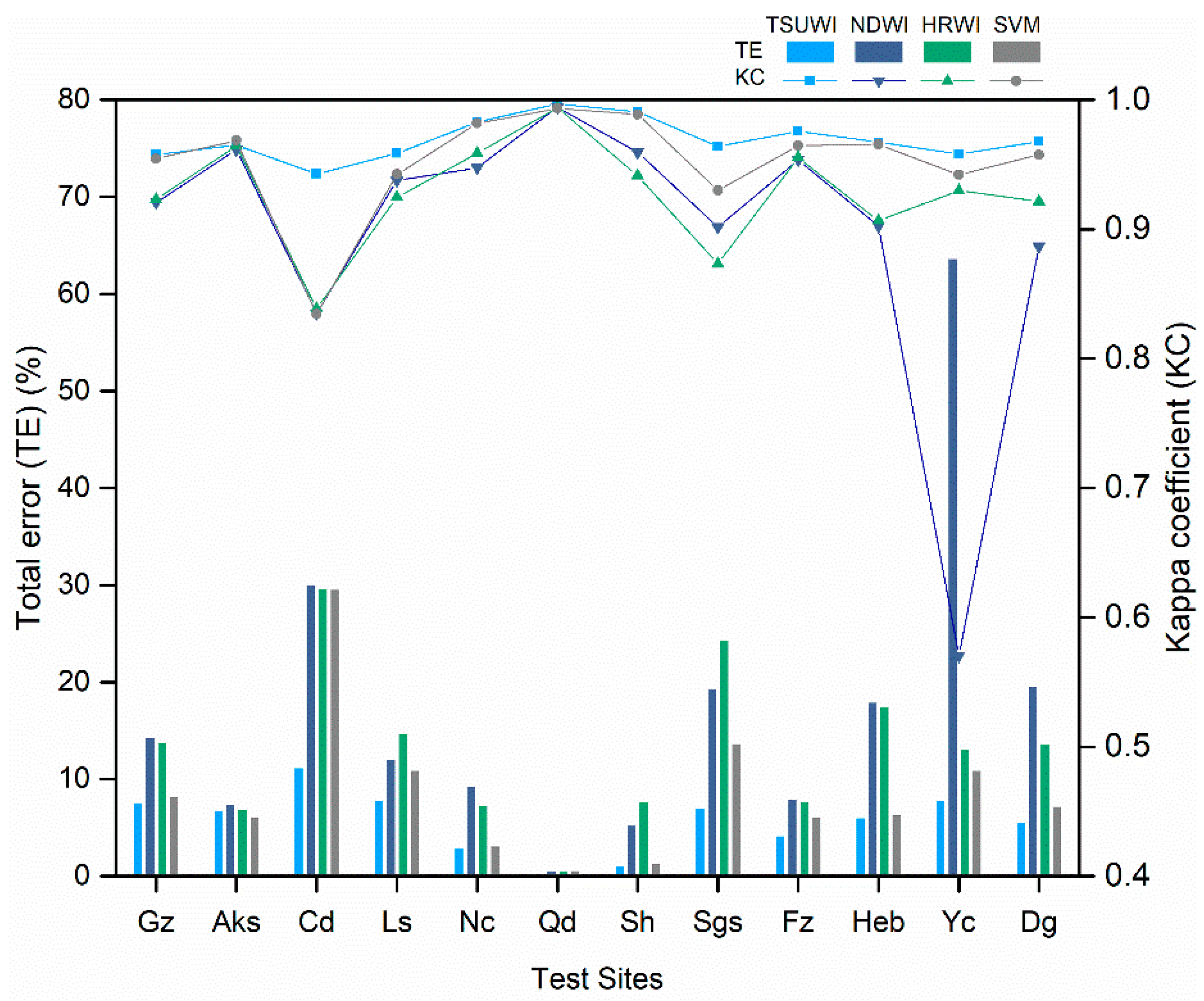
The water classification accuracies of the TSUWI, NDWI, HRWI, and SVM methods at the twelve sites are presented in Table 6. Statistical analysis of Table 6 indicated that the TSUWI successfully achieved high accuracy of urban surface water mapping at all test sites, with a mean KC equal to 0.97 and a mean TE (the sum of the CE and OE) of 5.82%. In contrast, the other three methods consistently exhibited lower classification accuracy, with an exception at the test site in Aksu for SVM (TE = 6.89% for TSUWI, while TE = 6.22% for SVM). The two conventional indexes, NDWI and HRWI, exhibited similar performance and resulted in a lower classification accuracy than the other two methods, and their mean KC and mean TE were 0.90, 17.41% and 0.93, 13.21%, respectively. The SVM classifier fell between, with a mean KC of 0.95 and a mean TE of 8.81%. For the overall stability, it clearly appeared that the classification accuracy of the TSUWI at different test sites exhibited smaller variations compared to the other three methods (Figure A1). By comparing the TEs at each test site, it is found that at most test sites, the TE of TSUWI was less than 55% of that of NDWI or HRWI and 85% of that of the SVM classifier (Figure A2). In other words, the proposed TSUWI could generally decrease the classification error by more than 45% compared to NDWI or HRWI, and 15% for the SVM.
Table 7 summarizes the significance of the accuracy difference at the twelve test sites by McNemar’s chi-square test. Overall, significant accuracy improvement was achieved by the TSUWI compared to the NDWI, HRWI, and SVM (p-value < 0.001). Exceptions were found in the test site in Aksu for the HRWI and SVM. At this site, the superiority of the TSUWI over the HRWI was nonsignificant (p-value = 0.364), and the TSUWI performed significantly worse than the SVM because the TE of the TSUWI (6.89%) was greater than that of the SVM, and the p-value was below 0.001.
4.3. Threshold Stability Analysis
A comparison of the stability of the optimal thresholds of the UWI, USI, NDWI, and HRWI is shown in Figure 5. The optimal thresholds of the UWI and USI at different test sites presented similar ranges, which were from −0.38 to 0.15 and −0.38 to 0.11, respectively. Compared to the NDWI and HRWI, the optimal thresholds of these two new indexes have smaller ranges of approximately 0. The maximum deviations of the optimal thresholds for the UWI and USI were both 0.38, whereas those for the NDWI and HRWI reached 0.56 and 0.85. It was concluded that the optimal thresholds of the UWI and USI at different test sites exhibited small variations from the default threshold of 0 compared to the NDWI and HRWI. Therefore, 0 could be used as the initial threshold in the iteration to find the optimum thresholds for both the UWI and USI.
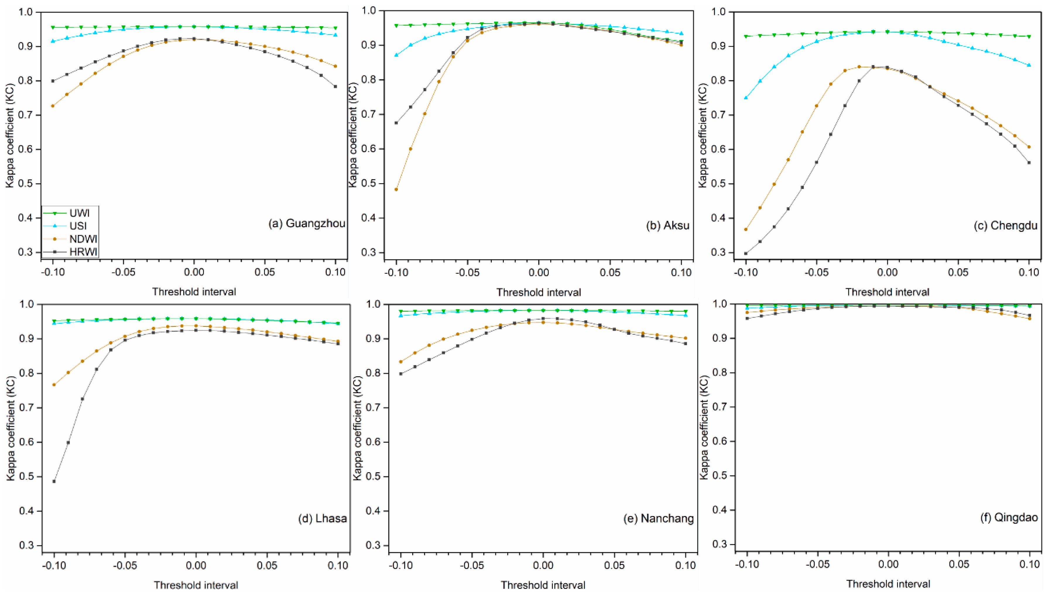
Figure 6 shows the accuracies of the UWI, USI, NDWI, and HRWI in the range of [−0.1, 0.1] near the optimal thresholds. At all twelve sites, the UWI exhibited almost unnoticeable variations, whereas the variations in the USI variation were relatively more obvious. This result means that the accuracy stability of the TSUWI near the optimal threshold is mainly dependent on that of the USI. In most cases, the accuracy of the USI is much more stable and higher than that of the NDWI and HRWI. Therefore, the TSUWI can alleviate the manual iteration issue for the optimum threshold, which is often normal and serious in the application of water indexes [40]. Moreover, the UWI can maintain the best performance in the range [−0.1, 0.1], while the USI can maintain the best performance in the range [−0.01, 0.01]. In the application of the TSUWI, we thus recommend 0.2 as the iteration step size for the UWI and 0.02 for the USI.
5. Discussion
5.1. Effects of Shadow Detection
The fact that shadows are widely distributed throughout urban areas and exhibit spectral patterns that are similar to those of water makes shadow removal a challenging problem in urban water extraction [25,41]. To address this issue, many researchers have contributed to previous research on the improvement of extraction accuracy by introducing additional shadow detection methods, such as object-oriented classification [35,42], shadow detection model based on SVM feature training [29], morphological shadow indexes [43,44] and invariant color model [45,46,47]. These methods may achieve expected results but are relatively difficult to apply and are time-consuming. Our new USI automatically suppresses shadow pixels through the arithmetic of bands. The circumvention of complex shadow detection procedures may simplify urban water mapping.
As shown in Section 3.3.4, the USI was preliminarily verified to have good separation through statistical analysis of pure pixels. To further confirm the role of this shadow detection index, we compared the accuracy results of the NDWI and HRWI, as well as their combination with the USI, and the proposed TSUWI at the twelve test sites (Table 8). Compared to the NDWI and HRWI, the combination of both with the USI achieved improved accuracy at each test site. For the NDWI and HRWI, the OE at most test sites was greater than the CE. The reason for this difference is that only the NDWI or HRWI cannot suppress the signal from shadows (Figure 2e,f), and the threshold has to be increased to achieve high accuracy at the cost of increasing the OE. By combining these indexes with the USI, the USI can successfully remove the noise from shadows (Figure 2h), and the NDWI or HRWI can then reduce the threshold to decrease the OE, thus resulting in improved accuracy. However, reducing the threshold of the NDWI (or HRWI) may simultaneously increase the number of misclassified pixels, such as dark built, asphalt and bright built (dark built and asphalt for HRWI) pixels, on which the USI also has limited effects (Figure 2h). Among the three combination methods with USI, the proposed TSUWI (UWI + USI) demonstrated the best performance with the highest accuracy in detecting urban water bodies at all test sites. Therefore, we recommend using the TSUWI method to extract urban water rather than the NDWI or the HRWI combined with the USI. However, the accuracies delivered by the combination of USI with NDWI and HRWI were quite similar to that of the TSUWI. This finding not only implies that the USI is much more important for the performance of the TSUWI, but also highlights the potential of USI to further improve the performance of other water indices.
5.2. Advantages of the Proposed Method
The TSUWI proposed in this paper contributes to the efforts to improve the accuracy of urban water extraction for various environmental studies. Although a number of improved water mapping indexes [22,24] have been proposed, few of them were established based on pure pixels derived from various water body types in various environments with a sufficient number of study sites. This method is constructed by combining the UWI and USI. To create effective indexes, a linear SVM model and numerous pure pixels were used in this study. As an outstanding machine learning technique for training the coefficient index, the linear SVM will not only provide an inherent default threshold of zero but also automatically achieve the largest separation between positive and negative classes [29]. The pure pixels were selected from eight sites located in different regions across China, which were deliberately chosen to cover various water body types and urban surfaces. As expected, the TSUWI was shown to extract urban surface water with high accuracy and remain robust for different types of water bodies under various urban environments.
The lack of a stable threshold is a problem in many water indexes, which may make the decision of a cut-off threshold more time-consuming and easily lead to a subjective choice of threshold with decreased accuracy [22]. In addition to accuracy improvement, the two indexes in the TSUWI were also shown to have a relatively stable optimal threshold that is close to zero and maintain good performance in the range of neighborhood thresholds near the optimal value. In the determination of optimal thresholds, 0 could be used as the starting point for the iterations for both the UWI and USI; 0.2 is recommended as the iteration step size for the UWI, and 0.02 is recommended for the USI. Benefiting from this, the application of this method is simplified, and the likelihood of achieving the highest urban water accuracy is improved. However, our findings are based on the suggestion that radiometric calibration and atmospheric correction were carefully undertaken for the images from all test sites. If either of these corrections is ignored, the accuracy and optimal thresholds may be different from those observed in this study.
Although high-resolution images have been available for a few decades, simple yet efficient indexes to characterize urban water extent with adequate detail are still lacking. This deficiency mainly results from the limited bands and surface noise in these images, which are often major causes of misclassification in urban surface water mapping. Our new TSUWI fills this gap. The TSUWI is calculated by the simple arithmetic of four standard bands prevalent at high resolution images. Using a simple threshold segmentation approach, the TSUWI consistently provides accurate water results in various water conditions with regard to depth, turbidity, chemical composition, and surface appearance. The extracted urban surface water can be further used as basic information for various urban studies, such as water quality analysis, urban heat island effect, and urban surface water change under the context of urbanization.
5.3. Further Improvements
Although the proposed TSUWI achieved satisfactory results in this study, some issues remain, such as atmospheric composition, transferability of the proposed method to other image data, seasonal variation in the angle of the sun, and seasonal behavior of water bodies themselves. All of these factors have an impact on the performance of the TSUWI. The use of different atmospheric correction methods may also influence thresholds and accuracies, especially when there is heavy haze. Heavy haze has been a serious issue in Chinese urban areas during wintertime in recent years. Current atmospheric correction models may not necessarily work well when correcting atmospheric haze. Therefore, one may need to consider the importance and type of atmospheric correction applied in the image preprocessing stage when evaluating the accuracies of different water extraction methods. Because the TSUWI is designed based on the land cover reflectance using GF-2 images, it is theoretically free of the constraints in terms of satellite image type with similar spectral bands. However, due to the inevitable differences among different sensors, it is still necessary to test the TSUWI on image data from other sources. Seasonal variation in the angle of the sun leads to changes in the brightness of images, and may also influence the performance of TSUWI. In addition, the spectral properties of water bodies will vary with seasonal changes in precipitation, biodegradability, domestic animals, and aquatic plants. In our test cases, we did not consider the influence of seasonal variation in the angle of the sun as well as the seasonal behavior of water bodies themselves. Therefore, the robustness of the new method also needs to be tested during different seasons. These issues are worth a follow-up study and verification.
6. Conclusions
The main purpose of this study was to devise a method that improves the accuracy of urban water extraction by increasing the spectral separability between water and non-water surfaces in the presence of shadows, which are often major causes of low classification accuracy. Using GF-2 data, we proposed an urban water extraction method called the TSUWI, which is a combination of two new indexes (UWI and USI) and compared its accuracy and threshold stability with that of the NDWI, HRWI, and SVM classifiers. In twelve cities across China, the accuracy assessment results showed that this method exhibited good performance, with an average KC of 0.97 and an average TE of 5.82%. Compared with the NDWI, HRWI, and SVM, the TSUWI generally exhibited improved accuracy by decreasing the TEs by more than 45% for the NDWI or HRWI and 15% for the SVM. In addition, both the UWI and USI were shown to have stable thresholds that were close to 0 and maintained good performance near their optimum thresholds with images from different locations and times compared to the NDWI and HRWI. Therefore, the TSUWI is an alternative and improved method for urban water mapping using high-resolution imagery. Moreover, the USI can be used alone to combine with other water indices for the further improvement of their performance in more accurate water extraction.
Supplementary Materials
The following are available online at https://www.mdpi.com/2072-4292/10/11/1704/s1, Table S1: List of water indexes. B, G, R and NIR refer to the surface reflectance of the green, red, blue and near infrared bands. SWIR1 and SWIR2 donate the surface reflectance of two shortwave infrared bands (band 5 and band7) in the Landsat TM/ETM+ imagery; Figure S1: Water extraction results using the TSUWI, NDWI, HRWI and SVM at the twelve test sites.
Author Contributions
W.W. provided the conception, conducted the data analysis, and wrote the manuscript. W.W., Q.L. and Y.Z. developed the methodology. Y.Z. revised the manuscript. X.D. and H.W. provided valuable insights and edited the manuscript.
Funding
This research is funded by the Special Scientific Research Fund of Public Welfare Profession of China (Grant No. 201511010).
Acknowledgments
Great thanks to the anonymous reviewers whose comments and suggestions significantly improved the manuscript.
Conflicts of Interest
The authors declare no conflict of interest.
Appendix A
Figure A1.
KCs and TEs obtained by the TSUWI, NDWI, HRWI and SVM for the twelve test sites. The twelve sites here were Guangzhou (Gz), Aksu (Aks), Chengdu (Cd), Lhasa (Ls), Nanchang (Nc), Qingdao (Qd), Shanghai (Sh), Shigatse (Sgs), Fuzhou (Fz), Haerbin (Heb), Yinchuan (Yc) and Dongguan (Dg).
Figure A1.
KCs and TEs obtained by the TSUWI, NDWI, HRWI and SVM for the twelve test sites. The twelve sites here were Guangzhou (Gz), Aksu (Aks), Chengdu (Cd), Lhasa (Ls), Nanchang (Nc), Qingdao (Qd), Shanghai (Sh), Shigatse (Sgs), Fuzhou (Fz), Haerbin (Heb), Yinchuan (Yc) and Dongguan (Dg).

Figure A2.
Total errors of the four methods for the twelve test sites.

References
- Kandulu, J.M.; Connor, J.D.; Macdonald, D.H. Ecosystem services in urban water investment. J. Environ. Manag. 2014, 145, 43–53. [Google Scholar] [CrossRef] [PubMed]
- Robitu, M.; Musy, M.; Inard, C.; Groleau, D. Modeling the influence of vegetation and water pond on urban microclimate. Sol. Energy 2006, 80, 435–447. [Google Scholar] [CrossRef]
- Bond, N.R.; Lake, P.S.; Arthington, A.H. The impacts of drought on freshwater ecosystems: An Australian perspective. Hydrobiologia 2008, 600, 3–16. [Google Scholar] [CrossRef]
- Yao, Y.; Zhang, Y.; Liu, J.; Shen, Z.; Liu, B. Model for evaluating urban water shortage risk: A case study in Beijing. Int. J. Digit. Content Technol. Appl. 2012, 6, 68–79. [Google Scholar]
- Vermonden, K. Key Factors for Biodiversity of Urban Water Systems. Ph.D. Thesis, Radboud University, Nijmegen, The Netherlands, 2010. [Google Scholar]
- Arnfield, A.J. Two decades of urban climate research: A review of turbulence, exchanges of energy and water, and the urban heat island. Int. J. Climatol. 2003, 23, 1–26. [Google Scholar] [CrossRef]
- Dong-Hai, L.I.; Bin, A.I.; Xia, L.I. Urban water body alleviating heat island effect based on RS and GIS: A case study of Dongguan City. Trop. Geogr. 2008, 28, 414–418. [Google Scholar]
- Jofre, J.; Blanch, A.R.; Lucena, F. Water-Borne Infectious Disease Outbreaks Associated with Water Scarcity and Rainfall Events. In Water Scarcity in the Mediterranean: Perspectives Under Global Change; Sabater, S., Barceló, D., Eds.; Springer: Berlin/Heidelberg, Germany, 2009; pp. 147–159. [Google Scholar]
- Kalnay, E.; Cai, M. Impact of urbanization and land-use change on climate. Nature 2003, 423, 528–531. [Google Scholar] [CrossRef] [PubMed]
- Mckinney, M.L. Urbanization as a major cause of biotic homogenization. Biol. Conserv. 2006, 127, 247–260. [Google Scholar] [CrossRef]
- Zhang, D.L.; Shou, Y.X.; Dickerson, R.R. Upstream urbanization exacerbates urban heat island effects. Geophys. Res. Lett. 2009, 36, 88–113. [Google Scholar] [CrossRef]
- Huang, S.L.; Chen, C.W. Urbanization and socioeconomic metabolism in Taipei. J. Ind. Ecol. 2010, 13, 75–93. [Google Scholar] [CrossRef]
- Morss, R.E.; Wilhelmi, O.V.; Downton, M.W.; Gruntfest, E. Flood risk, uncertainty, and scientific information for decision making: Lessons from an interdisciplinary project. Bull. Am. Meteorol. Soc. 2005, 86, 1593–1601. [Google Scholar] [CrossRef]
- Giardino, C.; Bresciani, M.; Villa, P.; Martinelli, A. Application of remote sensing in water resource management: The case study of Lake Trasimeno, Italy. Water Resour. Manag. 2010, 24, 3885–3899. [Google Scholar] [CrossRef]
- Lira, J. Segmentation and morphology of open water bodies from multispectral images. Int. J. Remote Sens. 2006, 27, 4015–4038. [Google Scholar] [CrossRef]
- Davranche, A.; Lefebvre, G.; Poulin, B. Wetland monitoring using classification trees and SPOT-5 seasonal time series. Remote Sens. Environ. 2012, 114, 552–562. [Google Scholar] [CrossRef] [Green Version]
- Sethre, P.; Rundquist, B.; Todhunter, P. Remote detection of prairie pothole ponds in the devils lake basin, North Dakota. Mapp. Sci. Remote Sens. 2005, 42, 277–296. [Google Scholar] [CrossRef]
- Asis, A.M.D.; Omasa, K.; Oki, K.; Shimizu, Y. Accuracy and applicability of linear spectral unmixing in delineating potential erosion areas in tropical watersheds. Int. J. Remote Sens. 2008, 29, 4151–4171. [Google Scholar] [CrossRef]
- Xie, H.; Luo, X.; Xu, X.; Pan, H.; Tong, X. Automated subpixel surface water mapping from heterogeneous urban environments using Landsat 8 OLI imagery. Remote Sens. 2016, 8, 584. [Google Scholar] [CrossRef]
- Bryant, R.G.; Rainey, M.P. Investigation of flood inundation on playas within the zone of Chotts, using a time-series of AVHRR. Remote Sens. Environ. 2002, 82, 360–375. [Google Scholar] [CrossRef]
- Jain, S.K.; Singh, R.D.; Jain, M.K.; Lohani, A.K. Delineation of flood-prone areas using remote sensing techniques. Water Resour. Manag. 2005, 19, 333–347. [Google Scholar] [CrossRef]
- Feyisa, G.L.; Meilby, H.; Fensholt, R.; Proud, S.R. Automated water extraction index: A new technique for surface water mapping using landsat imagery. Remote Sens. Environ. 2014, 140, 23–35. [Google Scholar] [CrossRef]
- Mcfeeters, S.K. The use of the normalized difference water index (NDWI) in the delineation of open water features. Int. J. Remote Sens. 1996, 17, 1425–1432. [Google Scholar] [CrossRef]
- Xu, H. Modification of normalised difference water index (NDWI) to enhance open water features in remotely sensed imagery. Int. J. Remote Sens. 2006, 27, 3025–3033. [Google Scholar] [CrossRef]
- Tong, X. New hyperspectral difference water index for the extraction of urban water bodies by the use of airborne hyperspectral images. Int. J. Remote Sens. 2014, 8, 085098. [Google Scholar] [Green Version]
- Verpoorter, C.; Kutser, T.; Tranvik, L. Automated mapping of water bodies using Landsat multispectral data. Limnol. Oceanogr. Methods 2015, 10, 1037–1050. [Google Scholar] [CrossRef]
- Gessner, M.O.; Hinkelmann, R.; Nützmann, G.; Jekel, M.; Singer, G.; Lewandowski, J.; Nehls, T.; Barjenbruch, M. Urban water interfaces. J. Hydrol. 2014, 514, 226–232. [Google Scholar] [CrossRef]
- Dare, P.M. Shadow analysis in high-resolution satellite imagery of urban areas. Photogramm. Eng. Remote Sens. 2005, 71, 169–177. [Google Scholar] [CrossRef]
- Yao, F.; Wang, C.; Dong, D.; Luo, J.; Shen, Z.; Yang, K. High-resolution mapping of urban surface water using ZY-3 multi-spectral imagery. Remote Sens. 2015, 7, 12336–12355. [Google Scholar] [CrossRef]
- Exelis. Exelis Visual Information Solutions. Available online: http://www.exelisvis.com (accessed on 15 November 2017).
- ExelisHelp. Exelis Visual Information Solutions. Available online: http://www.exelisvis.com/Support/HelpArticles.aspx (accessed on 15 November 2017).
- Tachikawa, T.; Kaku, M.; Iwasaki, A.; Gesch, D.B.; Oimoen, M.J.; Zhang, Z.; Danielson, J.; Krieger, T.; Curtis, B.; Haase, J. ASTER Global Digital Elevation Model Version 2—Summary of Validation Results; NASA: Pasadena, CA, USA, 2011.
- Kaufman, Y.J.; Remer, L.A. Detection of forests using mid-IR reflectance: An application for aerosol studies. Geosci. Remote Sens. IEEE Trans. 1994, 32, 672–683. [Google Scholar] [CrossRef]
- Neto, A.M.; Rittner, L.; Leite, N.; Zampieri, D.E. Pearson’s correlation coefficient for discarding redundant information in real time autonomous navigation system. In Proceedings of the 16th IEEE International Conference on Control Applications, Singapore, 1–3 October 2007. [Google Scholar]
- Yang, F.; Guo, J.; Tan, H.; Wang, J. Automated extraction of urban water bodies from Zymulti Log Pectral imagery. Water 2017, 9, 144. [Google Scholar] [CrossRef]
- Sun, J.; Li, Q.; Lu, W.; Wang, Q. Image recognition of laser radar using linear SVM correlation filter. Chin. Opt. Lett. 2007, 5, 549–551. [Google Scholar]
- Fu, Z.; Robles-Kelly, A.; Zhou, J. Mixing linear SVMs for nonlinear classification. IEEE Trans. Neural Netw. 2010, 21, 1963–1975. [Google Scholar] [PubMed]
- Provost, F.; Kohavi, R. Guest editors’ introduction: On applied research in machine learning. Mach. Learn. 1998, 30, 127–132. [Google Scholar] [CrossRef]
- Leeuw, J.D.; Jia, H.; Yang, L.; Liu, X.; Schmidt, K.; Skidmore, A.K. Comparing accuracy assessments to infer superiority of image classification methods. Int. J. Remote Sens. 2006, 27, 223–232. [Google Scholar] [CrossRef]
- Ji, L.; Zhang, L.; Wylie, B. Analysis of dynamic thresholds for the normalized difference water index. Photogramm. Eng. Remote Sens. 2009, 75, 1307–1317. [Google Scholar] [CrossRef]
- Xie, C.; Huang, X.; Zeng, W.; Fang, X. A novel water index for urban high-resolution eight-band Worldview-2 imagery. Int. J. Digit. Earth 2016, 9, 925–941. [Google Scholar] [CrossRef]
- Zhou, W.Q.; Huang, G.L.; Troy, A.; Cadenasso, M.L. Object-based land cover classification of shaded areas in high spatial resolution imagery of urban areas: A comparison study. Remote Sens. Environ. 2009, 113, 1769–1777. [Google Scholar] [CrossRef]
- Chen, Y.; Wen, D.; Jing, L.; Shi, P. Shadow information recovery in urban areas from very high resolution satellite imagery. Int. J. Remote Sens. 2007, 28, 3249–3254. [Google Scholar] [CrossRef]
- Huang, X.; Zhang, L. Morphological building/shadow index for building extraction from high-resolution imagery over urban areas. IEEE J. Sel. Top. Appl. Earth Observ. Remote Sens. 2012, 5, 161–172. [Google Scholar] [CrossRef]
- Tsai, V.J.D. A comparative study on shadow compensation of color aerial images in invariant color models. IEEE Trans. Geosci. Remote Sens. 2006, 44, 1661–1671. [Google Scholar] [CrossRef]
- Arévalo, V.; González, J.; Ambrosio, G. Shadow detection in colour high-resolution satellite images. Int. J. Remote Sens. 2008, 29, 1945–1963. [Google Scholar] [CrossRef]
- Chung, K.L.; Lin, Y.R.; Huang, Y.H. Efficient shadow detection of color aerial images based on successive thresholding scheme. IEEE Trans. Geosci. Remote Sens. 2009, 47, 671–682. [Google Scholar] [CrossRef]
Figure 1.
Locations of the twelve study sites and Gaofen-2 (GF-2) scenes in true color composites of red, green, and blue bands.
Figure 1.
Locations of the twelve study sites and Gaofen-2 (GF-2) scenes in true color composites of red, green, and blue bands.


Figure 2.
Distributions of reflectance and water index values (a–h) for the major urban land cover types, including bright soil, bright built, vegetation, black soil, asphalt, dark built, light shadow, dark shadow, and water. Horizontal lines in each box plot (boxes and whiskers) indicate the locations of the 10th, 25th, 50th, 75th, and 90th percentiles, and the circles indicate the 5th and 95th (blue dashed line) percentiles. The red dashed rectangles show the contrast between shadows and water in each water index. NIR: near-infrared; NDWI: Normalized Difference Water Index; HRWI: High Resolution Water Index; UWI: Urban Water Index; USI: Urban Shadow Index.

Figure 3.
Separability of dark shadows and water in the six band ratios, including NIR/G, NIR/R, NIR/B, B/G, G/R, and B/R, denoted by the amounts of pure water pixels that fell out of the area encompassed by the two dashed lines in each plot. (a–f) display the scatter plots of surface reflectance of pure dark shadow and water pixels. The slopes of the two dashed lines in each plot correspond to the 5th and 95th percentiles of the corresponding band ratios of pure dark shadow pixels, respectively.
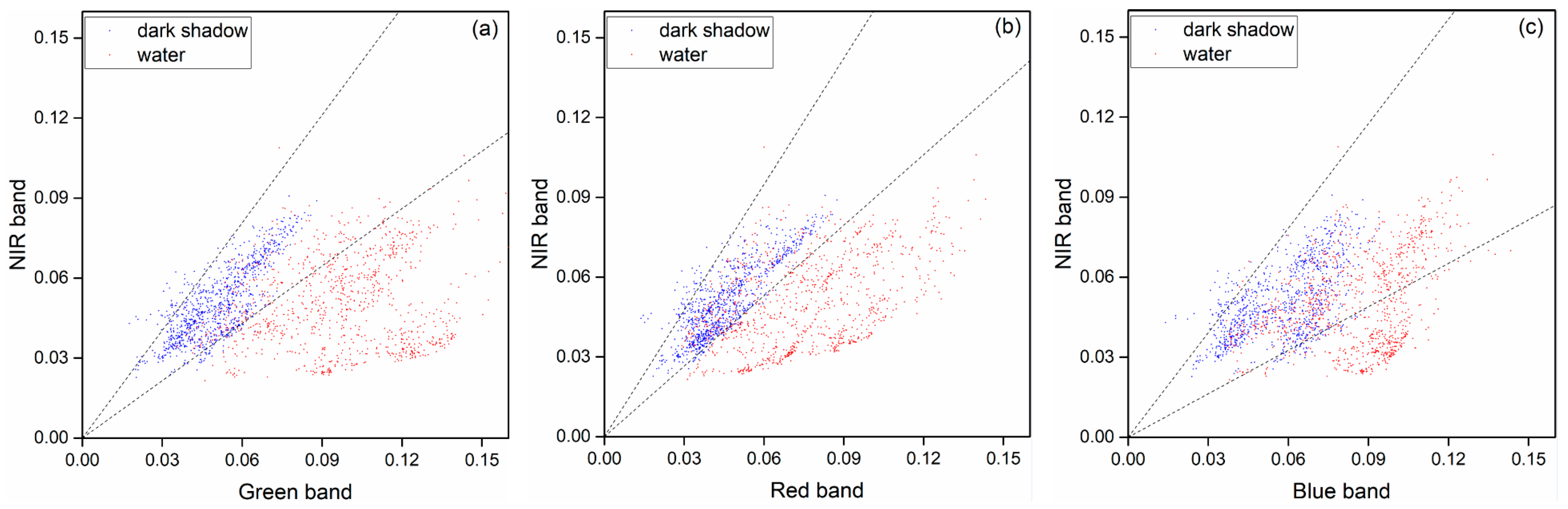

Figure 4.
Histograms of PUWI (a) and UWI (b) for pure pixels of positive classes (water and dark shadows) and negative classes (non-water types except dark shadows). The dashed gray lines indicate the peaks of the Gaussian fit curves.
Figure 4.
Histograms of PUWI (a) and UWI (b) for pure pixels of positive classes (water and dark shadows) and negative classes (non-water types except dark shadows). The dashed gray lines indicate the peaks of the Gaussian fit curves.

Figure 5.
Threshold variability and distribution of index values of water pixels for the UWI, USI, NDWI, and HRWI. Dashed lines show the maximum and minimum of the optimal threshold at the twelve test sites, and the “x” symbol shows the optimal threshold for each site.
Figure 5.
Threshold variability and distribution of index values of water pixels for the UWI, USI, NDWI, and HRWI. Dashed lines show the maximum and minimum of the optimal threshold at the twelve test sites, and the “x” symbol shows the optimal threshold for each site.

Figure 6.
The accuracies of the UWI, USI, NDWI, and HRWI at twelve test sites (a–i) in a range of thresholds near the optimal threshold: (a) Guangzhou; (b) Aksu; (c) Chengdu; (d) Lhasa; (e) Nanchang; (f) Qingdao; (g) Shanghai; (h) Shigatse; (i) Fuzhou; (j) Haerbin; (k) Yinchuan; (l) Dongguan.
Figure 6.
The accuracies of the UWI, USI, NDWI, and HRWI at twelve test sites (a–i) in a range of thresholds near the optimal threshold: (a) Guangzhou; (b) Aksu; (c) Chengdu; (d) Lhasa; (e) Nanchang; (f) Qingdao; (g) Shanghai; (h) Shigatse; (i) Fuzhou; (j) Haerbin; (k) Yinchuan; (l) Dongguan.


Table 1.
Characteristics of the twelve study sites.
| Study Sites | Main Water Types/Features | Location | Area (km2) | Topography | Climate |
|---|---|---|---|---|---|
| Guangzhou | River c,t/lake c/pond c,t,e | 23.11°N, 113.33°E | 574.9 | Plain/hills | Subtropical oceanic monsoon |
| Aksu | River c,n/lake s,t | 41.19°N, 80.31°E | 171.7 | Basin | Temperate continental arid |
| Chengdu | River c,t,n/pond c,t/reservoir c | 30.64°N, 104.11°E | 521.9 | Plain | Subtropical humid monsoon |
| Lhasa | River c,t/pond c | 29.67°N, 91.16°E | 54.0 | Mountain/plateau | Plateau mountain |
| Nanchang | River t,w/lake c,t/pond c,t,e/reservoir c,t | 28.69°N, 115.82°E | 516.2 | Plain/hills | Subtropical humid monsoon |
| Qingdao | Sea c/tidal creek t/river n,c,t/pond c,t | 36.13°N, 120.38°E | 561.8 | Plain/hills | Warm temperate monsoon |
| Shanghai | Harbor w,t /river c,t/lake c,t/pond c,t | 31.36°N, 121.55°E | 504.9 | Plain | Subtropical oceanic monsoon |
| Shigatse | River c,t/lake c,t/pond c,t | 29.25°N, 88.89°E | 84.0 | Mountain/plateau | Plateau mountain |
| Fuzhou | River c,t,w/lake c,t/pond c,t/reservoir c | 26.01°N, 119.30°E | 522.2 | Basin/hills | Subtropical oceanic monsoon |
| Haerbin | River t,w/lake c,t,e/ponds c,t,e | 45.71°N, 126.60°E | 468.3 | Plain | Temperate monsoon |
| Yinchuan | Lake c,t/river c,n/pond c,t | 38.48°N, 106.24°E | 525.1 | Plain | Temperate continental |
| Dongguan | River c,t/lake c,t/pond c,t,e/reservoir c | 22.98°N, 113.68°E | 288.9 | Plain/hills | Subtropical oceanic monsoon |
Note: c means clear water, t means turbid water, e means eutrophic water, n means narrow water, and w means wide water.
Table 2.
Basic characteristics of GF-2 satellite. NIR: near-infrared.
| Spectral Bands | Wavelength (μm) | Resolution (Nadir Point) | Swath Width | Side-Swing Ability | Revisit Cycle |
|---|---|---|---|---|---|
| Panchromatic | 0.45–0.90 | 0.8 m | 45 km | ±35° | 5 days |
| Band1—Blue | 0.45–0.52 | 3.2 m | |||
| Band2—Green | 0.52–0.59 | ||||
| Band3—Red | 0.63–0.69 | ||||
| Band4—NIR | 0.77–0.89 |
Table 3.
Characteristics of the twelve study sites.
| Study Sites | GF-2 Scene | Supplementary Reference Data | ||
|---|---|---|---|---|
| Acquisition Date | Path | Row | ||
| Guangzhou | 4 November 2016 | 1016 | 185 | Google Earth™ image acquired on 5 October/5 November/9 December 2016, ©Digital Globe |
| Aksu | 29 February 2016 | 102 | 135 | Google Earth™ image acquired on 17 April 2016, ©Digital Globe |
| Chengdu | 21 March 2015 | 27 | 164 | Google Earth™ image acquired on 11 February/21 March 2015, ©Digital Globe, CNES/Airbus |
| Lhasa | 3 December 2016 | 63 | 167 | Google Earth™ image acquired on 3 December 2016, ©Digital Globe |
| Nanchang | 28 November 2016 | 1013 | 170 | Google Earth™ image acquired on 24 September/1 December/31 December 2016, ©Digital Globe |
| Qingdao | 16 February 2016 | 1006 | 149 | Google Earth™ image acquired on 16 January 2016, ©Digital Globe |
| Shanghai | 2 January 2015 | 999 | 162 | Google Earth™ image acquired on 18 December 2014, and 24 January/18 February 2015, ©Digital Globe |
| Shigatse | 12 January 2017 | 69 | 168 | Google Earth™ image acquired on 21 May 2018, ©CNES/Airbus |
| Fuzhou | 7 December 2016 | 1001 | 177 | Google Earth™ image acquired on 21 January/1 March 2017, © Digital Globe, CNES/Airbus |
| Haerbin | 10 September 2015 | 997 | 122 | Google Earth™ image acquired on 19 June/9 July/16 September/24 October 2015, © Digital Globe |
| Yinchuan | 4 January 2017 | 27 | 142 | Google Earth™ image acquired on 30 October/2 November/ 13 November 2016, and 21 January 2017, ©Digital Globe |
| Dongguan | 15 February 2017 | 1015 | 186 | Google Earth™ image acquired on 12 February 2017, ©Digital Globe |
Table 4.
Separability of water and dark shadows in six band ratios using the M-statistical test.
| Class Pair | M Value | |||||
|---|---|---|---|---|---|---|
| NIR/G | NIR/R | NIR/B | B/G | G/R | B/R | |
| Water vs. Dark shadows | 1.12 | 0.87 | 0.65 | 0.91 | 0.57 | 0.24 |
Table 5.
Pearson’s Correlation Coefficient (PCC) among the six band ratios.
| Value | Band Ratio Pair | ||||||
|---|---|---|---|---|---|---|---|
| NIR/G vs. NIR/B | NIR/G vs. NIR/R | B/G vs. B/R | G/R vs. B/R | B/G vs. G/R | NIR/G vs. B/G | NIR/G vs. G/R | |
| Pearson’s r | 0.91 | 0.94 | 0.71 | 0.50 | −0.25 | 0.51 | −0.58 |
Table 6.
Summary of classification accuracies of the three methods by test site. TSUWI: Two-Step Urban Water Index; NDWI: Normalized Difference Water Index; HRWI: High Resolution Water Index; SVM: Support Vector Machine.
Table 6.
Summary of classification accuracies of the three methods by test site. TSUWI: Two-Step Urban Water Index; NDWI: Normalized Difference Water Index; HRWI: High Resolution Water Index; SVM: Support Vector Machine.
| Test Sites | Kappa Coefficient | Total Error (%) | ||||||
|---|---|---|---|---|---|---|---|---|
| TSUWI | NDWI | HRWI | SVM | TSUWI | NDWI | HRWI | SVM | |
| Guangzhou | 0.96 | 0.92 | 0.92 | 0.95 | 7.72 | 14.46 | 13.90 | 8.35 |
| Aksu | 0.97 | 0.96 | 0.96 | 0.97 | 6.89 | 7.58 | 7.07 | 6.22 |
| Chengdu | 0.94 | 0.84 | 0.84 | 0.83 | 11.33 | 30.15 | 29.75 | 29.70 |
| Lhasa | 0.96 | 0.94 | 0.92 | 0.94 | 7.97 | 12.16 | 14.84 | 11.05 |
| Nanchang | 0.98 | 0.95 | 0.96 | 0.98 | 3.11 | 9.45 | 7.41 | 3.28 |
| Qingdao | 1.00 | 0.99 | 0.99 | 0.99 | 0.34 | 0.65 | 0.69 | 0.75 |
| Shanghai | 0.99 | 0.96 | 0.94 | 0.99 | 1.24 | 5.38 | 7.80 | 1.48 |
| Shigatse | 0.96 | 0.90 | 0.87 | 0.93 | 7.10 | 19.43 | 24.51 | 13.81 |
| Fuzhou | 0.98 | 0.95 | 0.96 | 0.96 | 4.31 | 8.10 | 7.82 | 6.25 |
| Haerbin | 0.97 | 0.90 | 0.91 | 0.97 | 6.17 | 18.09 | 17.64 | 6.50 |
| Yinchuan | 0.96 | 0.57 | 0.93 | 0.94 | 7.97 | 63.79 | 13.25 | 11.04 |
| Dongguan | 0.97 | 0.89 | 0.92 | 0.96 | 5.65 | 19.69 | 13.78 | 7.33 |
Table 7.
Summary of McNemar’s χ2 test for accuracy difference between the TSUWI and the NDWI, HRWI and SVM.
Table 7.
Summary of McNemar’s χ2 test for accuracy difference between the TSUWI and the NDWI, HRWI and SVM.
| Test Sites | TSUWI vs. NDWI | TSUWI vs. HRWI | TSUWI vs. SVM | |||
|---|---|---|---|---|---|---|
| χ2 | p-Value | χ2 | p-Value | χ2 | p-Value | |
| Guangzhou | 132,839.0 | <0.001 | 115,749.6 | <0.001 | 3154.6 | <0.001 |
| Aksu | 77.3 | <0.001 | 0.8 | 0.364 | 93.6 | <0.001 |
| Chengdu | 17,469.1 | <0.001 | 16,782.9 | <0.001 | 29,634.9 | <0.001 |
| Lhasa | 789.6 | <0.001 | 1611.7 | <0.001 | 565.7 | <0.001 |
| Nanchang | 156,460.7 | <0.001 | 90,288.0 | <0.001 | 473.3 | <0.001 |
| Qingdao | 27,076.7 | <0.001 | 29,515.0 | <0.001 | 37,705.9 | <0.001 |
| Shanghai | 365,387.6 | <0.001 | 614,546.5 | <0.001 | 5523.5 | <0.001 |
| Shigatse | 5466.0 | <0.001 | 9882.5 | <0.001 | 2461.9 | <0.001 |
| Fuzhou | 93,062.7 | <0.001 | 82,875.6 | <0.001 | 33,324.0 | <0.001 |
| Haerbin | 146,443.9 | <0.001 | 148,493.8 | <0.001 | 474.1 | <0.001 |
| Yinchuan | 1,637,618.0 | <0.001 | 41,856.2 | <0.001 | 18,304.1 | <0.001 |
| Dongguan | 242,347.7 | <0.001 | 118,820.2 | <0.001 | 10,548.3 | <0.001 |
Table 8.
Summary of the accuracy using HRWI, NDWI, NDWI+USI, HRWI+USI and TSUWI (UWI+USI) at each optimal threshold.
Table 8.
Summary of the accuracy using HRWI, NDWI, NDWI+USI, HRWI+USI and TSUWI (UWI+USI) at each optimal threshold.
| Test Sites | NDWI | HRWI | NDWI + USI | HRWI + USI | TSUWI | ||||||||||
|---|---|---|---|---|---|---|---|---|---|---|---|---|---|---|---|
| Kappa | OE% | CE% | Kappa | OE% | CE% | Kappa | OE% | CE% | Kappa | OE% | CE% | Kappa | OE% | CE% | |
| Guangzhou | 0.92 | 10.22 | 4.24 | 0.92 | 10.68 | 3.22 | 0.93 | 9.08 | 3.46 | 0.95 | 5.84 | 3.48 | 0.96 | 5.37 | 2.35 |
| Aksu | 0.96 | 2.04 | 5.55 | 0.96 | 2.96 | 4.11 | 0.96 | 2.04 | 5.51 | 0.96 | 2.98 | 4.03 | 0.97 | 1.98 | 4.91 |
| Chengdu | 0.84 | 25.29 | 4.86 | 0.84 | 24.49 | 5.26 | 0.88 | 11.76 | 10.96 | 0.93 | 6.66 | 8.02 | 0.94 | 5.91 | 5.42 |
| Lhasa | 0.94 | 8.61 | 3.55 | 0.92 | 7.30 | 7.55 | 0.95 | 7.42 | 3.27 | 0.94 | 7.32 | 4.09 | 0.96 | 6.68 | 1.30 |
| Nanchang | 0.95 | 6.15 | 3.30 | 0.96 | 4.43 | 2.98 | 0.96 | 3.72 | 2.64 | 0.97 | 2.66 | 2.19 | 0.98 | 1.99 | 1.11 |
| Qingdao | 0.99 | 0.35 | 0.31 | 0.99 | 0.33 | 0.36 | 1.00 | 0.19 | 0.33 | 0.99 | 0.19 | 0.38 | 1.00 | 0.17 | 0.17 |
| Shanghai | 0.96 | 2.05 | 3.33 | 0.94 | 3.25 | 4.55 | 0.99 | 0.92 | 0.45 | 0.99 | 0.86 | 0.47 | 0.99 | 0.83 | 0.41 |
| Shigatse | 0.90 | 10.80 | 8.63 | 0.87 | 7.51 | 17.00 | 0.91 | 9.67 | 7.50 | 0.91 | 9.17 | 8.23 | 0.96 | 3.83 | 3.28 |
| Fuzhou | 0.95 | 6.64 | 1.46 | 0.96 | 6.05 | 1.77 | 0.96 | 5.93 | 1.65 | 0.97 | 3.69 | 2.01 | 0.98 | 3.05 | 1.25 |
| Haerbin | 0.90 | 13.60 | 4.49 | 0.91 | 9.67 | 7.98 | 0.91 | 11.39 | 4.49 | 0.92 | 9.55 | 4.67 | 0.97 | 4.20 | 1.97 |
| Yinchuan | 0.57 | 7.93 | 55.86 | 0.93 | 9.23 | 4.02 | 0.96 | 5.42 | 2.70 | 0.96 | 6.14 | 1.89 | 0.96 | 5.41 | 2.56 |
| Dongguan | 0.89 | 7.54 | 12.16 | 0.92 | 8.09 | 5.69 | 0.97 | 3.38 | 2.61 | 0.96 | 3.72 | 3.01 | 0.97 | 3.04 | 2.61 |
© 2018 by the authors. Licensee MDPI, Basel, Switzerland. This article is an open access article distributed under the terms and conditions of the Creative Commons Attribution (CC BY) license (http://creativecommons.org/licenses/by/4.0/).
Share and Cite
MDPI and ACS Style
Wu, W.; Li, Q.; Zhang, Y.; Du, X.; Wang, H. Two-Step Urban Water Index (TSUWI): A New Technique for High-Resolution Mapping of Urban Surface Water. Remote Sens. 2018, 10, 1704. https://doi.org/10.3390/rs10111704
AMA Style
Wu W, Li Q, Zhang Y, Du X, Wang H. Two-Step Urban Water Index (TSUWI): A New Technique for High-Resolution Mapping of Urban Surface Water. Remote Sensing. 2018; 10(11):1704. https://doi.org/10.3390/rs10111704
Chicago/Turabian StyleWu, Wei, Qiangzi Li, Yuan Zhang, Xin Du, and Hongyan Wang. 2018. "Two-Step Urban Water Index (TSUWI): A New Technique for High-Resolution Mapping of Urban Surface Water" Remote Sensing 10, no. 11: 1704. https://doi.org/10.3390/rs10111704
Note that from the first issue of 2016, this journal uses article numbers instead of page numbers. See further details here.