Comparison of Digital Building Height Models Extracted from AW3D, TanDEM-X, ASTER, and SRTM Digital Surface Models over Yangon City


1
Institute of Industrial Science, The University of Tokyo, Tokyo 153-8505, Japan
2
Graduate School of Environmental Earth Science, Hokkaido University, Sapporo 060-0808, Japan
*
Author to whom correspondence should be addressed.
Remote Sens. 2018, 10(12), 2008; https://doi.org/10.3390/rs10122008
Submission received: 25 October 2018
/
Revised: 2 December 2018
/
Accepted: 8 December 2018
/
Published: 11 December 2018
(This article belongs to the Special Issue Remote Sensing based Building Extraction)
Abstract
:Vertical urban growth in the form of urban volume or building height is increasingly being seen as a significant indicator and constituent of the urban environment. Although high-resolution digital surface models can provide valuable information, various places lack access to such resources. The objective of this study is to explore the feasibility of using open digital surface models (DSMs), such as the AW3D30, ASTER, and SRTM datasets, for extracting digital building height models (DBHs) and comparing their accuracy. A multidirectional processing and slope-dependent filtering approach for DBH extraction was used. Yangon was chosen as the study location since it represents a rapidly developing Asian city where urban changes can be observed during the acquisition period of the aforementioned open DSM datasets (2001–2011). The effect of resolution degradation on the accuracy of the coarse AW3D30 DBH with respect to the high-resolution AW3D5 DBH was also examined. It is concluded that AW3D30 is the most suitable open DSM for DBH generation and for observing buildings taller than 9 m. Furthermore, the AW3D30 DBH, ASTER DBH, and SRTM DBH are suitable for observing vertical changes in urban structures.
1. Introduction
Urban areas in the 21st century are facing growing challenges from natural and man-made crises. These include chronic stresses, like environmental pollution and climate change, and acute shocks, like floods and earthquakes. Urban risk assessment maps and appropriate land-use profiles are needed to increase the resilience of our cities to these disasters [1]. Vertical urban growth or urban volume is one such evolving measure of an urban land-use profile [2]. Traditionally, building heights were assessed from maps showing the floor-area ratio derived from land transaction cases and land-use update surveys [3], statistical yearbooks [4], aerial photos, and local agency-supplied maps [5]. Increasingly, digital building height models (DBHs) generated from remote sensing techniques are becoming a popular technique for monitoring the urban environment. Digital building heights have several applications, such as modeling urban expansion [5], extracting and reconstructing buildings [6], simulating air pollution dispersion [7], estimating energy consumption [8] and solar potential [9], observing heat islands [10], flood hazard zoning [11], assessing GPS performance [12], and many others. Furthermore, if building heights from different time periods are available, they can also provide information about policy effects on horizontal and vertical urban growth [3,4,13].
Digital building height (DBH) is extracted from a digital surface model (DSM). A DSM is obtained from airborne laser scanning [14], high-resolution stereo image pairs [15], or interferometric SAR (synthetic aperture radar) pairs [16]. Of these technologies, airborne laser scanning (ALS) has the highest accuracy in parameterizing building morphology, ranging from simple footprint identification [17] to complicated 3D structure and roof plane modeling [14,18]. State-of-the-art ALS approaches have also achieved very high accuracy in complex urban environments by integrating aerial imagery [19], city administrative data [20], architectural knowledge [21], and the Big Data approach [22].
Despite these promising results, there have been relatively few published studies on such methods being applied to large areas [23]. Furthermore, ALS data sources and aerial images are often under the control of government ministries, and, due to high operational costs, they are not available in many parts of the world [24]. Since several such regions are also undergoing rapid urban growth and will potentially face the associated adverse environmental impacts and safety concerns, it is necessary to monitor their urban volumes or building heights. At the same time, the quality and quantity of satellite images as well as the capabilities of sophisticated algorithms for DSM and DBH computations have increased dramatically in recent years [25]. Although such high-resolution satellite datasets are available for a fraction of the cost compared with ALS data, they are prohibitively expensive to obtain at the global scale. Despite various applications for building height data, there is still no such global dataset available that is comparable to the ‘Global Rural-Urban Mapping Project (GRUMP) Urban Extents Grid, v1’ [26,27] or the ‘Global Urban Heat Island (UHI)’ dataset [28]. Being able to derive building heights at a global scale is crucial not only for places that lack access to such data but also for global climate model simulations Zhang et al. [29], population distribution mapping [30], and other useful applications. Fortunately, freely available but coarse-resolution global DSMs, such as SRTM (Shuttle Radar Topography Mission), ASTER (Advanced Spaceborne Thermal Emission and Reflection Radiometer), and AW3D30 (ALOS (Advanced Land Observing Satellite) World 3D 30 m Resolution DSM) also exist, and they present an attractive opportunity to explore their application to urban areas. Presently, open DSMs are used mostly for large-scale regional geomorphological studies, such as earthquake and flood inundation modeling, among others. [31]. Studies have compared and revealed the relative merits of open DSMs of diverse geomorphological terrains [32,33,34,35] as well as urban areas [36]. However, the effectiveness of using open DSMs for urban applications is largely unexplored, so it is unclear whether the established accuracies of open DSMs would translate to similar accuracies of their corresponding DBHs.
The possibility of extracting building heights from open DSMs was first alluded to by Nghiem et al. [37] with regard to using SRTM for large-scale area mapping. When the SRTM DSM was examined in Los Angeles by Gamba et al. [38] and in Baltimore City by Quartulli and Datcu [39], they concluded that the SRTM digital elevation model (DEM) could be used for detecting tall buildings. Since then, other global DSMs, including AW3D30, TanDEM-X (TerraSAR-X Add-On for Digital Elevation Measurements), and ASTER Global DEM (GDEM), have also been shared publicly, but it is not clear whether they are suitable for the detection and estimation of DBHs. Each DSM has a different acquisition period and acquisition method. For example, AW3D and TanDEM-X were acquired around the early 2010s, while ASTER and SRTM were acquired in the early 2000s. This affects what can be ‘seen’ in these DSMs. Given what is available, this decadal period could be significant for studying 3D urban changes in rapidly growing cities [40,41,42]. Although the DSMs AW3D30 and TanDEM-X are known to be vertically more accurate than ASTER and SRTM, a DBH comparison is needed to establish the extracted height accuracy and its limitations. With sufficient accuracy, the models could be deployed at a global scale. To the best of the authors’ knowledge, only Wang et al. [43] has attempted to address these challenges so far.
Objective
The objective of this study was to compare the accuracy of digital building heights (DBHs) extracted from open DSMs (AW3D30, ASTER, and SRTM).
2. Methodology
The flowchart of the datasets and methodology used for DBH estimation and comparison is shown in Figure 1. Briefly, the AW3D5 digital building height model (DBH) was validated with respect to the GeoEye DBH and TanDEM-X DBH, the degradation of the height accuracy from the fine-resolution AW3D5 DBH to the coarse-resolution AW3D30 DBH was assessed, and the terrain model was compared with the AW3D30, ASTER, and SRTM DBHs.
2.1. Study Site
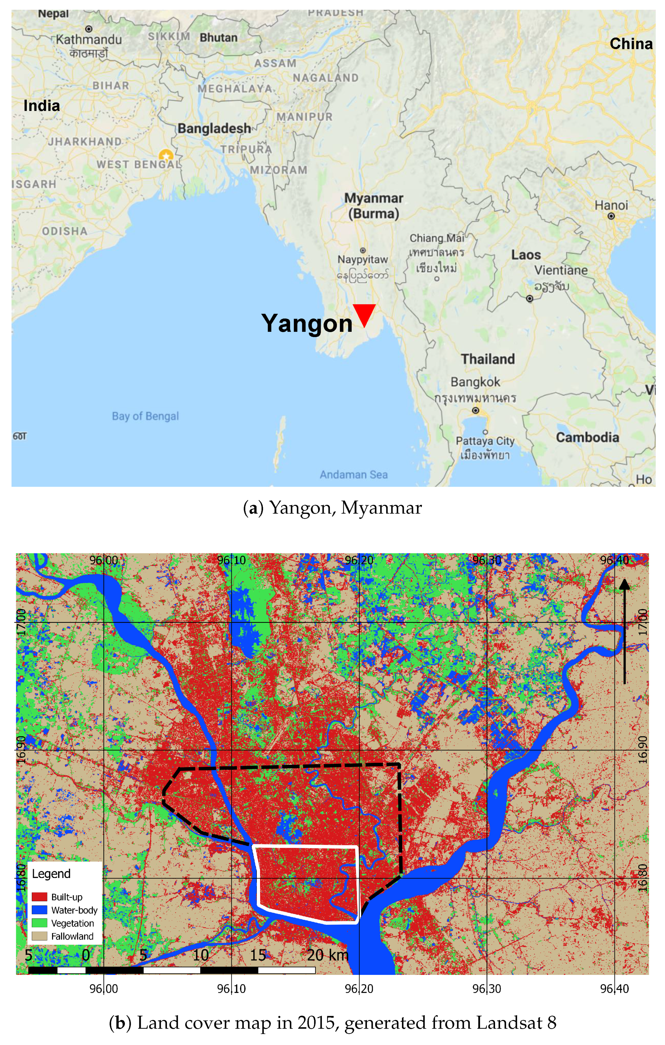
Yangon city (Figure 2a), the former capital of Myanmar, was selected as the study area due to its intense urban expansion within the last two decades. As per the 2014 Myanmar population census [44], urban Yangon has 5.16 million inhabitants. This is an increase of 85% over 1983 estimates. In roughly the same period between 1979 to 2009, Yangon’s urban area experienced about a 5-fold expansion [45], most of which took place within the last decade. Apart from this, Yangon lies in one of the world’s most disaster-prone countries. Yangon is situated on hilly terrain surrounded by a river and is at high risk of earthquakes and floods. The country was affected by Cyclone Nargis in 2008 and the Shan State Earthquake in 2011, which displaced several thousand people. Alarmingly, simulations of future urban expansion have shown that development will continue in flood-prone and earthquake-risk areas [46]. A land cover map of Yangon that shows built-up areas, water-bodies, vegetation, and fallow land for the year 2015 is presented in Figure 2b. Land cover types were classified using cloud-free Landsat-8 surface reflectance imagery available in Google Earth Engine [47]. In this paper, the fallow-land class refers to non-cultivated agricultural land and other bare lands, while the vegetation class refers to both forests and agricultural land with crops. Central Yangon has seen vertical expansion in the form of the construction of several new buildings alongside the older industrial, residential areas and colonial buildings. Rapid horizontal expansion has taken place from the center to periphery, stretching the built-up boundary.
2.2. Data Used
SRTM: The Shuttle Radar Topography Mission (SRTM) DEM was an international effort led by NASA and NGA (US National Geospatial Agency). The DSM was processed from C-band and X-band radar imagery collected from two antennae atop the Space Shuttle in an 11-day mission in February 2000 [48] and had an absolute vertical accuracy of less than 9 m [49]. Until 2014, the global dataset was available at a 3-arcsecond posting for regions outside of the US. In 2015, the LP DAAC (Land Processes Distributed Active Archive Center) released the NASA SRTM Version 3.0 Global 1-arcsecond dataset (SRTMGL1) [50]. At a global scale, the 1-arcsecond version (SRTMGL1) has the same root-mean-square error (RMSE) of 10.3 m as its 3-arcsecond version [51]. Its RMSE ranges from 5.9 m in urban areas to 10.4 m in bushland [32,52]. In this research, the 1-arcsecond (approximately 30 m at the equator) SRTMGL1 was used and is subsequently referred to as SRTM. It is available from NASA’s Earth Explorer website [53].
ASTER: Advanced Spaceborne Thermal Emission and Reflection Radiometer (ASTER) Global Digital Elevation Model Version 2 (GDEM V2) dataset is a DSM from NASA and Japan’s Ministry of Economy, Trade and Industry (METI). It is freely available at a 1-arcsecond posting from NASA’s Earth Explorer. The DSM was generated from nadir and backward-looking visible and near-infrared imagery from the ASTER sensor aboard NASA’s Terra satellite. It was compiled from over 1.5 million scenes acquired between 2000 and 2009 and released in 2011 [54]. GDEM V2 is an improved version of the earlier GDEM V1 in terms of spatial resolution and coverage, water body mask, and horizontal and vertical accuracy [55]. Still, it contains disturbances in the values due to an increased frequency of noise on account of using a smaller correlation kernel to enhance the horizontal resolution. The RMSE accuracy of the ASTER GDEM changes with location [32,56] and is influenced by the land cover type, varying from 15.1 m in forested mountainous areas [54] to 23.3 m in urban areas [57]. In this study, ASTER GDEM V2 was used and is further referred to as ASTER.
TanDEM-X: TanDEM-X (TerraSAR-X Add-On for Digital Elevation Measurements) was launched in 2010 by the German Aerospace Center (DLR) with the aim of generating WorldDEM, a consistent global DSM. Its identical twin, TerraSAR-X, was launched earlier in 2007, and both satellites collect microwave imagery with X-band single-polarized SAR antennae. A uniqueness of this mission is that data collection takes place in a bistatic mode, in which both the satellites orbit with a short baseline and acquire data at the same location and same time. This helps to greatly reduce the effects of atmospheric disturbances. Marconcini et al. [58] demonstrated promising results of building height extraction over the Yellow River Delta, China using preliminary TanDEM-X DEM. Wessel et al. [59] validated the 12 m resolution TanDEM-X DEM with GPS measurements scattered over the United States and established its RMSE accuracy for urban (1.4 m) and vegetation areas (1.8 m). Its vertical RMSE over the mostly urban Tokyo was evaluated as 3.2 m [60], with higher errors occurring over built-up and vegetation classes. The final WorldDEM is publicly available at a 90 m resolution. The 12 m and 30 m resolution versions are freely available for research proposals (through DLR) and are priced for commercial use (through Airbus Defence and Space company). As part of a research project, a pair of TanDEM-X HH polarization images in ascending orbit were acquired in StripMap mode (ground spatial resolution between 2 and 3 m) for 6 September 2011. The incidence angle of the master image was 44.57 with a height of ambiguity of 50.14 m. A 12 m TanDEM-X InSAR DSM was generated in [60] and upsampled to a 5 m resolution for comparison with other DSM products.
AW3D: The ALOS World 3D (AW3D©JAXA) DSM, publicly released by JAXA in 2016, is the most recent DSM considered in this paper. The AW3D DSM was generated using images from PRISM’s (Panchromatic Remote-Sensing Instrument for Stereo Mapping) front, nadir, and backward-looking panchromatic bands aboard ALOS (Advanced Land Observing Satellite). PRISM sensors were in operation between 2006 and 2011 and acquired imagery at a 2.5 m resolution which was processed with a 5 m grid spacing to generate a global elevation dataset, AW3D [61]. The AW3D DSM is commercially distributed at a 5 m resolution, while a 30 m downsampled dataset (known as ‘AW3D30’) is publicly available. The AW3D DSM generally meets the 5 m RMSE target height accuracy as per its producers [61]. However, Takaku et al. [61] found slope-dependent errors, with errors greater than 5 m occurring for slope angles larger than 30 degrees. Using longitudinal profiles of airport runways, Caglar et al. [62] found that AW3D30 has an RMSE of 1.78 m and contains an elevation anomaly due to sensor noise and the processing algorithm. Takaku et al. [61] found a mostly positive bias, while Caglar et al. [62] identified a negative bias in elevation estimation. In the Philippines, AW3D30’s RMSE varies from 4.3 m in urban areas to 6.8 m in areas with dense vegetation [32]. Estoque et al. [63] found that heights filtered from the AW3D5 DSM are more accurate for lower buildings (e.g., ground truth building height <100 m) in less dense cities than for high-rise buildings and denser cities. In this research, a commercial 5 m DSM [64] was obtained as part of the research project, while the freely distributed 30 m AW3D DSM was downloaded from [65]. The 5 m resolution and 30 m resolution AW3D DSMs are henceforth referred to as AW3D5 and AW3D30, respectively.
Reference data: Ideally, the heights obtained from ground control points should be used as references. A higher-resolution surface model can also be used as a reference when ground control data are unavailable [66]. A high-resolution DSM was generated from 0.5 m resolution commercial GeoEye-1 stereo image pairs acquired in 2013 over Yangon. The DSM was then resampled to 4 m using PCI Geomatica 2015 software. The digital terrain model (DTM) was extracted by the in-built Wallis filter, which is a local adaptive filter that is useful for areas with significant shadow. The DSM generated with GeoEye-1 image pairs has a vertical RMSE accuracy ranging from 0.57 m in flat areas to 0.87 m in urban areas [67]. The completeness of the DSM in urban areas is 63.23% due to occlusion resulting from a high base/height (B/H) ratio (ratio of the image-pair distance to the height of the sensor) and the convergence angle of the imaging geometry [67]. In the pair used in this research, the stereo images also had different acquisition times that affected the quality of the generated DSM over some locations. For example, inaccurate matching was generated over the pagodas constructed with metallic roof plates, as they appeared differently in the stereo-pair due to the changed sun-view angle. This led to improper registration and erroneous height estimation.
Stable structures: Since open DSMs (AW3D30, ASTER, and SRTM) were acquired in different years, their DBHs cannot be compared directly in a fast-developing city like Yangon. To overcome this limitation, ‘stable structures’ were identified for comparison. These structures are those buildings that were consistently present between 2003 and 2011 and can be identified visually from historical imagery in Google Earth Pro software. The year 2003 is the earliest year for which high-resolution optical imagery is available. Care was taken to select only those structures that appear without any errors in the GeoEye DBH. In total, 52 ‘stable structures’ were identified, which included large pagodas and temples, colonial buildings, a palace, government offices, a sports complex, large hotels, and residential apartments. Some examples are shown in Figure 3. A polygon was drawn manually around each stable structure’s footprint.
All DSMs used in this research are summarized in Table 1. All DSMs and DBHs were referenced to the World Geodetic System (WGS84) horizontal datum and Earth Gravitational Model 1996 (EGM96) vertical (geoid) datum. A highly accurate image registration that is precise to each pixel is desirable for comparison. Since the DSMs were originally not georegistered with each other, we co-registered each DSM and DBH with the reference GeoEye DSM. Thirty ground control points for high-resolution DSMs and 15 tie-points spread evenly over the study area were selected for each co-registration. This was performed in the map registration module of the software ENVI4.7 (Exelis Visual Information Solutions, Boulder, CO, USA) using a rotation, scaling, and translation technique, followed by cubic convolution resampling. Separate co-registration of DSMs and DBHs was done to prevent the influence of interpolation on height estimation.
2.3. DBH Generation
There are several types of building extraction based on the desired or possible details, ranging from building footprints to building roof contours [23]. As per the study objective and data limitations, the focus was on building height extraction. A DBH is different from a digital building model (DBM), which is a more comprehensive 3D representation of buildings and includes all aspects of the building geometry [6]. DBH is considered a normalized DSM (nDSM) over built-up class pixels. An nDSM is calculated as the difference in elevation values between the DSM and DTM (digital terrain model, also known as a bare earth model). The extraction of an nDSM requires distinguishing ground from non-ground pixels by generating a DTM. Most algorithms first generate the DTM from a photogrammetric DSM by identifying pixels which are part of the local terrain [68]. There are several methods for identifying non-ground pixels, but they often assume that the terrain is smooth and that a large height difference exists between neighboring ground and non-ground points [69]. Deep learning approaches have resulted in high-accuracy building extraction (overall accuracy > 95%), with very high resolution imagery [70,71]. However, these networks are designed for small-sized images (e.g., 256 × 256 pixels, 512 × 512 pixels, etc.) to prevent memory overloading, which can produce discontinuous artifacts [72]. Many such models rely on a fully connected neural network [73], which is a pre-trained model using an RGB image repository (Imagenet [74]) and exploit similar features between the RGB intensities and the depth images, such as edges, corner, and end-points [72]. In the case of a coarse-resolution DSM, such features are not clearly visible, and we were skeptical of their performance with coarse resolution. Recognizing these possible limitations, a morphological approach—a multi-directional processing and slope-dependent filtering technique called ‘MSD filtering’ [75]—was used for DTM generation in light of its consideration of the terrain slope and overall simplicity in implementation [69]. The MSD filtering technique is an extension of a similar technique developed for an ALS DSM [76]. MSD filtering is effective over hilly terrains with slopes for extracting a DTM with a sub-meter high-resolution DSM [75]. An enhancement of MSD filtering, the ‘network of ground points’ technique, also exists [77] and does not need to consider the slope angle. However, as admitted by Mousa et al. [77], this probably holds true only for very high resolution DSMs. Therefore, we implemented the MSD method instead of the ‘network of ground points’ method. MSD filtering has also been used to generate a DTM for the alignment of high-resolution optical and SAR images in urban areas [78].
The MSD filtering technique requires four parameters to generate a DTM: the Gaussian smoothing kernel size, the scanline filter extent, the height threshold, and the slope threshold. Each DSM pixel was checked to determine whether it should be considered ground by comparing it with other pixels within the predefined neighborhood scanline filter extending in eight directions. If the pixel was identified as a ground pixel in more than five directions, it was labeled as a terrain pixel by the majority voting method. To draw the comparison, a local reference terrain slope was first generated by 2D Gaussian smoothing. Then, the pixel’s height was compared with the lowest elevated pixel within the scanline filter extent. If this height difference was more than the height threshold parameter, the pixel was classified as a non-ground pixel. Then, if the slope difference between the current and the successive pixel in the scanline direction was greater than the slope threshold, it was labeled as a non-ground pixel. If the slope was positive and less than the slope threshold, then that pixel was given the same label as its previous pixel. Otherwise, that pixel was labeled as ground. This resulted in a raster with only ground points and holes, the latter being locations where non-ground points exist. Thereafter, a linear interpolation technique from the ‘SciPy’ module of Python [79] was used to fill the holes for generating the DTM. The nDSM was generated by subtracting the DTM from its DSM.
Parameter Selection
The GeoEye nDSM was used as a reference to choose suitable parameter values for the scanline extent, height threshold, and slope threshold. The parameters for the Gaussian smoothing filter were set to a 100 m kernel size and a 25 m standard deviation to generate the initial local terrain. After trying various combinations of height difference thresholds and slope thresholds, 3 m and 30 were chosen, respectively, as they captured the greatest number of structures. A 3 m height difference threshold approximately corresponds to a one-story construction. A lower value of the height difference threshold leads to underestimation, while higher values lead to an overestimation of the ground terrain. One drawback to the MSD scanline approach arises when no ground pixels lie within the eight directional scanlines [77]. This can happen when a structure is contiguous and larger than the scanline extent. The neighborhood scanline filter extent parameter was stretched beyond 100 m for a greater chance of successfully ‘finding’ a ground pixel. This ensured more chances to observe a ground pixel within the scanline since any contiguous urban structure is unlikely to be larger than 100 m in all scanline directions.
The AW3D5 nDSM was generated with a scanline extent of 300 m, a height threshold of 3 m, and a slope threshold of 30. Setting a lower value for the scanline filter extent (<300 m) underestimated the structures’ footprints and also their heights, e.g., a scanline extent of 150 m resulted in a lesser overall mean height estimation by 0.2 m when compared with the DBH generated with a scanline filter extent of 300 m. This was more pronounced for tall structures. Similarly, the TanDEM-X nDSM was generated with a scanline extent of 100 m, a height threshold of 3 m, and a slope threshold of 30. The same parameters used for AW3D5 were deemed fit to extract the nDSM from AW3D30 and ASTER GDEM v2. Due to the low differentiation between ground and non-ground points in SRTM, the height threshold parameter was lowered to 2 m. In the AW3D5 and TanDEM-X nDSMs thus generated, about 10% of the pixels had negative heights, out of which 90% of the values were between m and 0 m. In the SRTM, ASTER, and AW3D30 nDSMs, 20% of the pixels had negative values, out of which 90% were between m and 0 m. These negative heights were removed.
2.4. Vertical Accuracy Assessment
There are several accuracy metrics for roof level and roof plane level evaluations [80]. Recent additions include shape similarity and positional accuracy metrics [81] and a threshold-free metric based on the overlap between extracted and reference roof planes [80]. However, the coarse DBH imposes limitations due to which such advanced metrics cannot be applied. For example, in a 30 m gridded DBH, roof planes are not visible except on very large structures that span several hundred meters. Therefore, pixel-based and object-based height accuracies were evaluated with conventional statistical metrics. Object-based heights were derived as mean pixel heights within the footprint polygon of each stable structure. The vertical accuracy of the estimated datasets (DBH and DTM) was analyzed by calculating the descriptive statistics of the difference between the estimated height and the reference height. These statistics were the root-mean-square error (RMSE), mean error (ME), mean absolute error (MAE), and standard deviation (SD). The RMSE describes how much the estimated dataset differs from the reference dataset in terms of deviation from zero. The ME describes the bias toward underestimation (negative ME) or overestimation (positive ME) with respect to the reference dataset. The SD represents the distribution of errors from the mean error (for normally distributed errors, the mean error is zero). So, a low SD value means less variation in error magnitudes. For any DBH or DTM, was extracted from DSM D with an image containing n pixels or objects, and its error metrics with respect to the reference DBH or DTM were calculated as shown in Equations (1)–(4).
Finally, in accordance with Rutzinger et al. [82], the correspondence of a building footprint within the stable structure polygon was checked pixel-wise. For this method, true positive (, when the footprint exists in the reference as well as in the DBH), false negative (, when the footprint is incorrectly identified as ground), true negative (, when the footprint is correctly identified as ground), and false positive (, when a ground pixel is identified as a footprint) pixels within each stable structure polygon were identified. The completeness and correctness was computed according to Equations (5) and (6).
where denotes the number of pixels.
3. Results and Discussion
3.1. Comparison of AW3D5 and TanDEM-X DBH
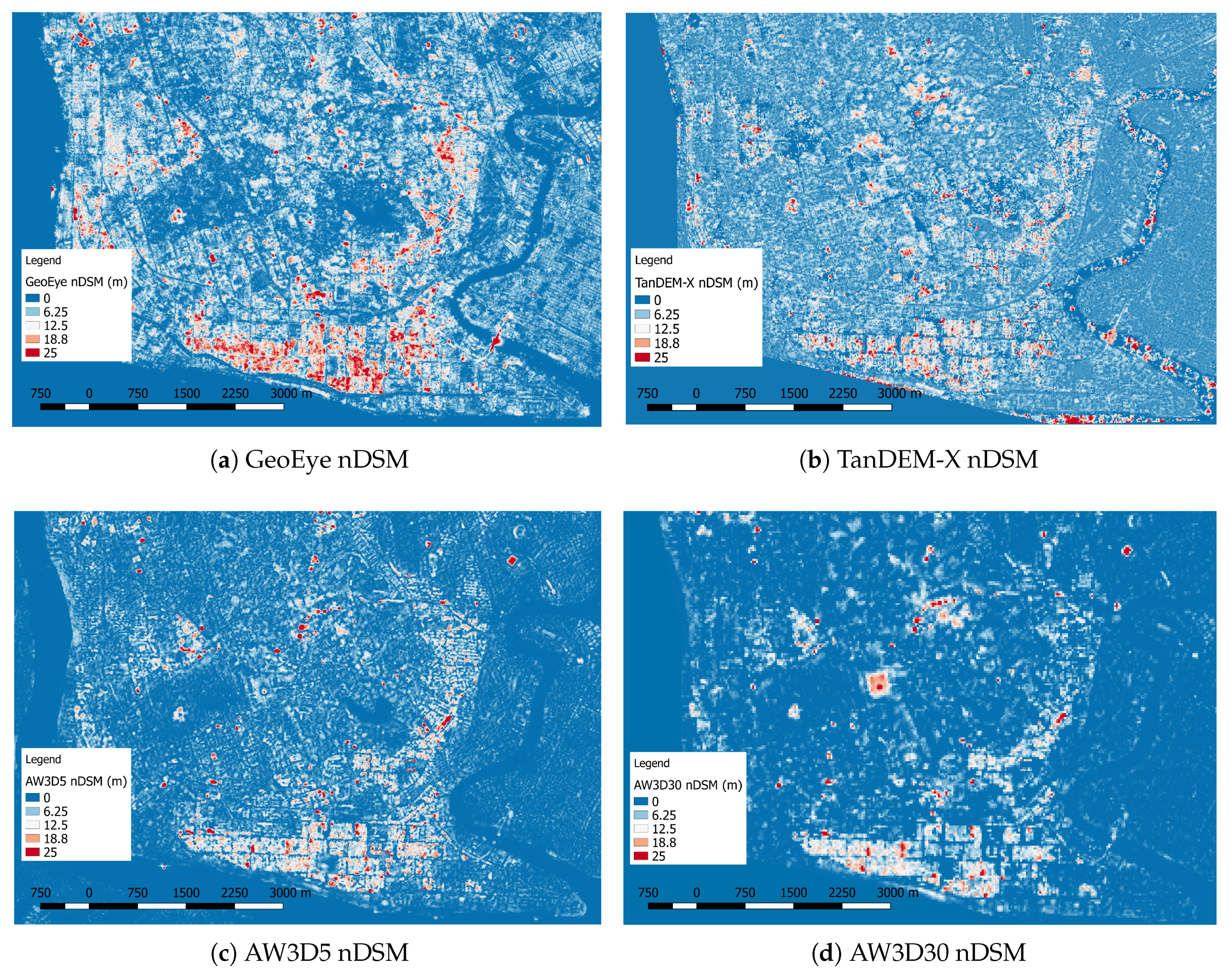
The AW3D5 DBH and TanDEM-X DBH along with the GeoEye DBH are shown in Figure 4. Also, the profiles at three example locations (A, B, and C) for the DSMs and DBHs from AW3D5, TanDEM-X, and the reference DBH are shown in Figure 5. Location A contains low-height buildings, while location C contains relatively taller buildings. Location B in Figure 5c shows a hilly terrain consisting of Yangon’s most important historic landmark, the Shwedagon Pagoda (distance mark: 580 m). It is a conical structure situated atop the highest elevated location. A visual comparison showed that compared with the GeoEye DBH, the AW3D5 DBH underestimated the height of single-story buildings, which were generally 3–4 m tall (in the Eastern portion of Figure 4c), but it better captured the heights of tall structures (in the Southern portion of Figure 4c). Generally, the TanDEM-X DBH had a similar profile trend to that of the AW3D5 DBH but did not capture the heights of tall structures. In the TanDEM-X DSM, and consequently, in its DBH, some skyscrapers and pagodas appeared as a tall inclined wall immediately followed by a hole. Since such locations were not flagged by TanDEM-X’s data consistency mask, it can be assumed that this is due to the local phase unwrapping errors that result in shadows or noise [83]. Many shadow pixels were also observed in tall buildings due to layover that resulted in incomplete footprints, ‘ramps’, and overall height underestimation. Also, buildings located along the azimuth direction were severely affected by layover issues. On the other hand, short structures were devoid of such artifacts. The reference GeoEye DBH also showed buildings that were missed due to the incorrect registration of high-resolution stereo-pairs over tall structures on account of occlusion, shadows, or high parallax error [84,85], although there were far fewer in number than those missed by the TanDEM-X DBH. The accuracies of the AW3D5 and TanDEM-X DBHs with respect to the GeoEye DBH are shown in Table 2. For the AW3D5 DBH, built-up areas had an RMSE of 3.55 m. This RMSE almost corresponds to the single-story high structures often seen in residential areas. The AW3D5 DBH had a negative ME ( m), which points to an underestimation bias by AW3D5. This implies that height estimation from AW3D5 over residential areas is unreliable. Further, some locations with tall buildings had large height differences on account of the low GeoEye accuracy, as seen in Figure 4 and Figure 5e (distance mark: 580 m). So, it is possible that the RMSE of the AW3D5 DBH could be even lower than 3.55 m if a more accurate reference DBH were used. Nonetheless, this value is within the desired producer RMSE of 5 m. The TanDEM-X DBH captured more short height structures (height < 5 m) than did the AW3D5 DBH. Its accuracy measures were slightly better than those of the AW3D5 DBH in all respects except the SD (Table 2). Its almost zero ME but positive MAE could also point to a higher occurrence of random errors. Overall, the AW3D DBH provided a slightly higher RMSE (by 0.21 m), lower ME (by 1.51 m), lower MAE (by 0.12 m), and lower SD (0.15 m). The AW3D5 DBH also identified more tall buildings in densely built-up areas than did TanDEM-X DBH. However, this comparison is based on the TanDEM-X DSM generated from a single pair of images. With the use of TanDEM-X’s final DEM which combines multiple acquisitions, better results can be expected.
One interesting aspect is the base/height (B/H) ratio, which is defined as the ratio of the stereo-pair separation to the height of the sensor. A high B/H leads to improved vertical accuracy [86]. However, in a dense urban setting, a high B/H leads to increased occlusion and poor matching [87]. The PRISM imagery (from which the AW3D DSM was generated) had a higher B/H ratio of 1.0 than the GeoEye imagery, whose B/H ratio varied from 0.54 to 0.83. GeoEye also has a high off-nadir look angle (10–35) to provide fast and varied acquisition, which is likely to result in slanted buildings due to the perspective view. This suggests that in the AW3D5 DBH, a higher vertical accuracy is achieved at the cost of more occlusion, while the reverse is true for the GeoEye DBH.
3.2. Accuracy Loss in AW3D DBH with Resolution Degradation
Profile sections of the AW3D5 and AW3D30 DBHs derived from the original DSM (not co-registered with the GeoEye DBH to preserve original height) are shown in Figure 6. The AW3D30 DBH showed similar height variation to that of AW3D5 but in a much coarser fashion. Due to the coarseness of the AW3D30 DBH, fewer ground points were preserved, especially in street canyons between buildings. This inhibits identification of individual buildings compared with the case of the AW3D5 DBH. This can be seen in Profile A (Figure 6) at the 100 m and 500 m distance marks. Pixels over those locations are more likely to be considered non-ground, leading to a height overestimation when there is a sudden steep change in ground elevation. This is why at location B (Figure 6), the AW3D30 DBH showed a higher height immediately preceding (distance mark: 550 m) or following (distance mark: 700 m) a relatively tall structure (Shwedagon Pagoda, distance mark: 600 m).
Another concern of note is the impact of mixed pixels arising from the pixel grid when AW3D5 is downsampled to AW3D30. Several instances were observed when buildings in the AW3D5 DBH with a ground footprint of approximately 30 m or less was split into adjacent 30 m resolution pixels, each with a lower height than the original. An example is shown (Figure 7), where a 30 × 30 m sized building was split into two pixels in the AW3D30 DBH. This is an unavoidable consequence of downsampling, and the split buildings appear to have less height in the 30 m resolution compared with the 5 m resolution. This can be seen in the original DSMs as well. This suggests that tall adjacent pixels seen in the AW3D30 DBH may have a smaller ground footprint than is estimated by the model.
The descriptive statistics for the AW3D30 DBH with the AW3D5 DBH downsampled with a mean filter as a reference highlighted the effect of coarse resolution (Table 3). The RMSE of the AW3D30 DBH was impacted only slightly (by 0.79 m) over the original AW3D5 DBH. The ME and MAE were m and 0.18 m, respectively, which points to a minor underestimation by the AW3D30 DBH. This could be due to the mixed-pixel issue highlighted in the previous paragraph. The non-visibility of several street canyons in the AW3D30 DBH could also have contributed to the SD.
3.3. Comparison of DTMs from AW3D30, ASTER, and SRTM
The different acquisition time periods of the AW3D30, ASTER, and SRTM DSMs resulted in dissimilar DBHs due to surface changes over time. To ensure a robust comparison, the DTMs extracted from the DSMs were compared to assess the agreement between the three DTMs. This was performed by land cover types: built-up, vegetation, and fallow land. Only the DTM values for those pixels with the same land cover types in both the Landsat 7 (2001) and Landsat 8 (2015) images were considered. The DTM over the complete area shown in Figure 2b was considered so as to ensure sufficient representation of all land cover types. Comparison plots are shown in Figure 8. In general, low-elevation pixels (≤10 m) mostly belonged to fallow land and vegetation, mid-elevation pixels (10–30 m) belonged to built-up areas, and high-elevation areas (≥30 m) were mixed between vegetation and built-up areas. The SRTM and AW3D30 DTMs were fairly consistent with each other, having a low overall RMSE (1.85 m) with a high correlation of 0.97. Comparatively, the ASTER DTM showed a higher overall RMSE with AW3D30 (3.12 m) and SRTM (4.03 m) and a lower correlation with AW3D30 (0.88) and SRTM (0.87). From Figure 8b, it can be seen that ASTER overestimated low-elevation pixels but underestimated high-elevation pixels. The ASTER DTM over built-up pixels located at a higher elevation was underestimated compared with AW3D30 and could be a cause of the DBH inaccuracy in those regions. This suggests the presence of systematic errors, which could be locally resolved by the calibration of the ASTER DTM. Comparison of the DTMs over vegetation was inconsistent, resulting in the highest RMSE compared with the other classes. In the SRTM DTM, this was due to the C-band SAR sensor, which can penetrate the leaf foliage, resulting in a lower DSM elevation than that in the DSM from optical sensors. In built-up areas, the DTMs of AW3D30 and SRTM were more consistent with each other than they were with the ASTER DTM, as can be seen by their RMSE values in Table 4. The ASTER DTM had a lower RMSE (3.18 m) compared with vegetation (RMSE: 3.72 m) and fallow land (RMSE: 3.24 m) with respect to the AW3D30 DTM.
3.4. Comparison of DBHs from AW3D30, ASTER, and SRTM
The DSM and DBH profiles of the SRTM, ASTER, AW3D30, and GeoEye DBHs are shown in Figure 9. To ensure comparison at the 30 m resolution, the GeoEye DBH was downsampled using a mean kernel and is henceforth referred to as GeoEye. The SRTM DBH had a similar trend to the AW3D30 DBH with large height underestimations. Although, originally, the SRTM DSM was intended to identify natural topography, and man-made features are mostly absent, some buildings can still be identified in the SRTM DBH. The SRTM DBH mostly hovered around 0 m except when a large structure or several tall buildings with heights greater than 10 m in GeoEye DBH were present. The ASTER DBH also underestimated structure heights but was closer to the AW3D30 DBH and GeoEye DBH than it was to the SRTM DBH. It can be seen in Figure 9b that over the Shwedagon Pagoda stable structure (distance mark: 600 m), the maximum height was estimated by the AW3D30 DBH (31 m), followed by the ASTER DBH (14 m) and SRTM DBH (11 m). There were several locations where the ASTER DBH estimation was higher than that of the AW3D30 DBH and GeoEye DBH. This can be seen in Figure 9b at the distances marked 400 m and at 1100 m. In the former case, it is due to the nDSM generating the algorithm; in the latter, it is the presence of noise in the original ASTER DSM itself that contributed to overestimation.
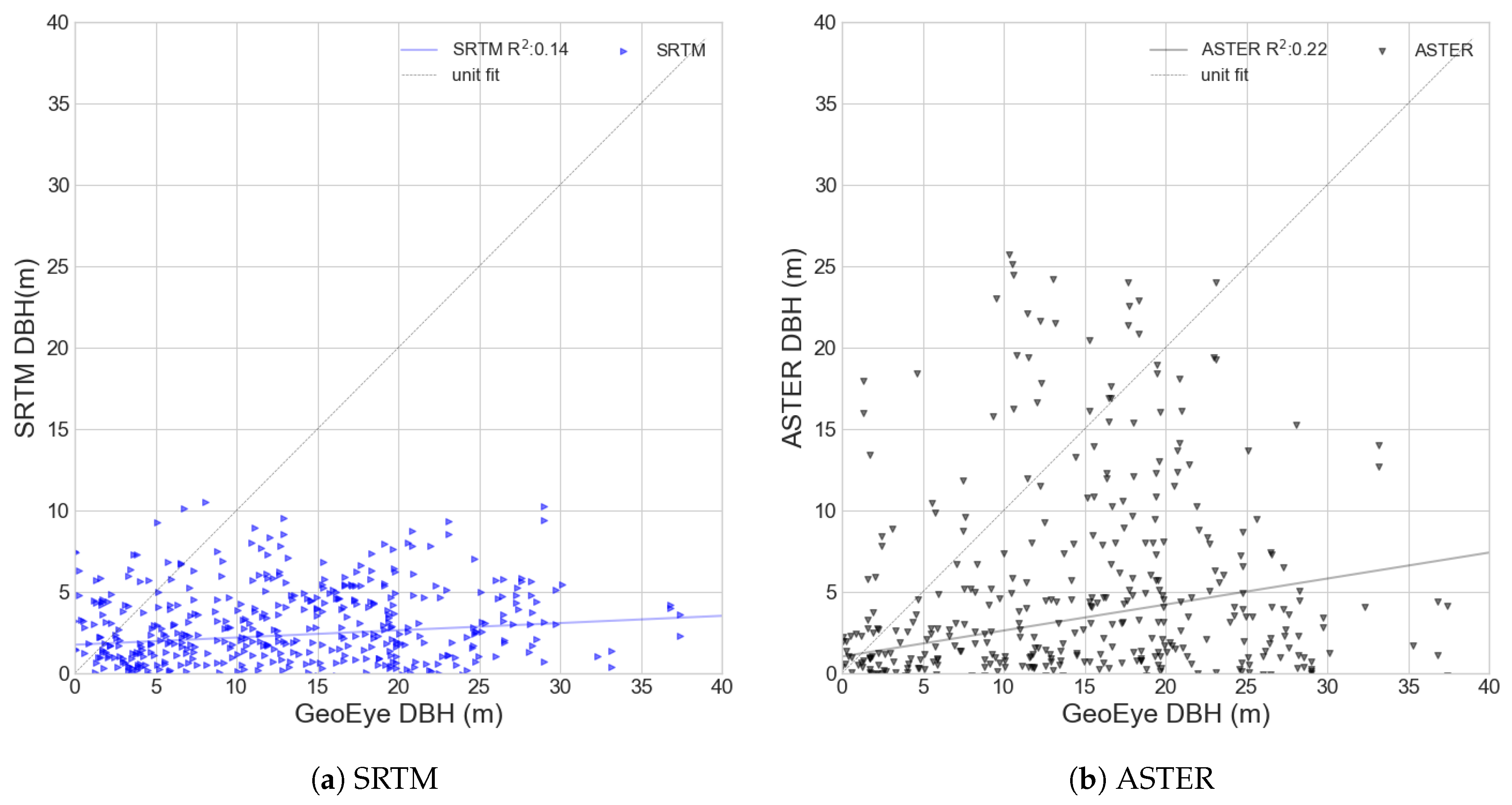
The statistical comparison of DBHs over stable structure pixels from the open DSMs and GeoEye is shown in Table 5. It is noteworthy that the mean pixel height of the AW3D30 DBH (ME: 9.14 m) was significantly higher than that of SRTM (ME: 3.10 m) and ASTER (ME: 5.49 m). The SDs of the AW3D30 DBH (6.40 m) and ASTER DBH (6.08 m) were closer to that of the GeoEye DBH (8.19 m) and much higher than that of SRTM (2.24 m), implying that the AW3D30 DBH and ASTER DBH show good variation in building heights. However, the high SD for the ASTER DBH may also be on account of noise generating anomalous heights. Along with the results of the previous section, we can conclude that a good agreement between a pair of DTMs does not imply a good agreement between their DBHs, e.g., SRTM and AW3D30 had a high correlation (0.97) but vastly different SD values. When pixel-based comparisons were made with GeoEye DBH, the ME values of the AW3D30 DBH and ASTER DBH were much lower than their MAE values. This, along with the sign of the ME, indicates that the AW3D30 DBH and ASTER DBH consistently underestimated the reference heights. This can also be seen in the scatterplots in Figure 10a–c. The coefficient of determination was low for the SRTM DBH (R: 0.14) and ASTER DBH (R: 0.22) but relatively high for the AW3D30 DBH (R: 0.60). This suggests that ASTER building heights were indeed noise artifacts, while the AW3D30 DBH represented reference building heights with some underestimation. The locations where the SRTM DBH was low (<0.3 m) despite high values in the GeoEYE DBH (>25 m) were checked. Such pixels belonged to dense neighborhoods with sloped metal-roofed buildings. On the other hand, a high SRTM DBH (>8 m) was estimated over large buildings with red brick or tiled rooftops. It is possible that shadowing and layover originating from sloped rooftops resulted in underestimation. The pixel locations where the AW3D30 DBH overestimated height compared with GeoEye were also probed. Such pixels belonged to locations with dense tall buildings and also those buildings where the footprint in GeoEye was smaller than the actual footprint. Interestingly, the RMSE of the AW3D30 DBH (8.69 m) with respect to GeoEye was not much degraded over its 5 m resolution version, i.e., the AW3D5 DBH (RMSE: 5.04 m). Assuming that a single-story building is about 3 m high, the RMSE of the AW3D30 DBH suggests that the AW3D30 DBH pixels can detect the height of buildings taller than 9 m or three stories.
Some instances of minor spatial misregistration (shift of 1–2 pixels) between the DBH datasets persisted despite several georegistration attempts. To overcome this limitation, object-based comparison of the mean height of each individual stable structure was performed. The summary of the statistics is shown in Table 5, and the scatterplot is shown in Figure 10d. The RMSE and MAE improved by about 2 m for each DBH when object-level statistics were computed. In Figure 10d, four outlying building heights can be seen for AW3D30, where the GeoEye DBH is between 7 and 12 m and the AW3D30 DBH is between 18 and 22 m. On closer inspection, it was found that these buildings were affected by blurring and small footprints in the GeoEye DBH. From the original GeoEye stereo image, we noticed that, in reality, these buildings were 6–10 stories high. This was determined by visually identifying the number of windows in the vertical direction. This suggested that the AW3D30 DBH was possibly correct over those locations, and the removal of these outlying building estimates increased the R to 0.62. The object-based RMSE of the AW3D30 DBH (6.92 m) suggests that if building footprints are already known, the AW3D30 DBH is suitable for the height estimation of buildings taller than two stories.
Regarding the average completeness of the building footprint, buildings in the AW3D30 DBH were 85.34% complete, followed by SRTM (82.12%), and ASTER (64.82%). This suggests that the AW3D30 DBH detected building footprints with a sufficiently high degree of completeness. Surprisingly, the SRTM DBH had a similar completeness rate to that of AW3D30, both of which were much better than that of ASTER DBH. This suggests the utility of the SRTM DBH in estimating the presence of buildings, although at a much lower height estimation. Upon examining the buildings with low footprint completeness, it was found that these mainly consisted of buildings with complicated rooftop structures and conical pagodas. However, each DBH product was affected to different extents by these complications. This is likely due to feature and intensity matching errors from complicated rooftop reflectance during the production of the original DSM. The use of the three images was effective in reducing such errors during DSM generation compared with using only two images [88]. The ASTER DBH could be severely affected by this factor, as its DSM was generated from only paired images compared with the triplet images used for AW3D DSM generation. It was not possible to compute the correctness satisfactorily, as buildings in the coarse DBH were clearly separated from each other, resulting in unrealistically high values.
Since the DBH generated from the DSMs were acquired during different time periods, this points to the possibility that vertical growth can be observed where it has taken place. A tall building at the 580 m distance mark in Figure 9c is clearly visible in the AW3D30 DBH but is absent in the ASTER and SRTM DBHs. After visual inspection of historical imagery with Google Earth, it was found that this particular building was constructed after 2005. Another tall building can be seen at the 850 m distance mark in Figure 9a in the AW3D30 DBH and SRTM DBH but not in the ASTER DBH. It is one of the stable structures, as identified from Google Earth’s historical imagery. Furthermore, there were several buildings that were present in the AW3D30 DBH and ASTER DBH but absent in the SRTM DBH. They can be seen at the distance marked from 500 to 700 m in Figure 9a and at the distance marked from 200 to 300 m in Figure 9c. These buildings were constructed after 2004, which explains their absence from the SRTM DBH. These examples also suggest that the ASTER DBH contained buildings built between the years 2004 and 2005. However, if a building seems to be present in the SRTM DBH but absent from the ASTER DBH, then the building is indeed present on the ground, and its absence from the ASTER DBH can be explained by errors in the ASTER DSM itself.
3.5. Discussion
In this paper, a simple approach to the extraction and comparison of DBHs without the use of any supporting datasets was used. It is possible that other methodologies may result in significantly better estimates of RMSE. So far, only one other study has extracted building heights from the same DSM sources as those used in this study. Wang et al. [43] derived building heights at a country-wide scale in the UK by using ALS building heights as training data in a random forest classifier. Their approach indicated that the highest accuracy was found with SRTM (R: 0.67), followed by ASTER (R: 0.66) and AW3D30 (R: 0.63), each with an RMSE lower than 1.9 m. This is interesting for two reasons: first, their coefficient of determination (R) for the AW3D30 DBH was quite close to that obtained in this study (R: 0.60) with a simpler technique. Second, Wang et al. [43] also achieved high accuracy for DBHs derived from SRTM and ASTER, which suggests that these datasets should not be discounted for DBH estimation. The results of this study could be biased on two clear accounts. First, the height accuracy was compared only with the DBH filtered from GeoEye, which has its own shortcomings. Furthermore, photogrammetric DSMs have limitations owing to spatial resolution, atmospheric errors, and matching errors, leading to erroneous heights at times. A more robust benchmarking of the results for rooftops could be achieved with a high-quality dense DBH obtained from an airborne ALS sensor, as it has a small footprint and high point density [83]. Second, the comparisons were performed with only 52 stable structures. These structures were mostly either tall buildings or prominent religious or colonial structures located in relatively less dense areas. It is possible that these structures biased the accuracy judgment in favor of the open DSMs. Comparison over a sufficiently large number of diverse stable structures could help to overcome this limitation.
The DSMs used in this study were based on images that are about a decade to two old. Even the latest available DSM used (TanDEM-X) has images from the year 2011. The relative importance of these datasets depends on the location under study, e.g., they are useful for studying urban growth in cities such as Yangon, Manila, and Shanghai that have seen rapid expansion during this period compared with already established cities, such as Tokyo and Seoul [89]. Nonetheless, future open DSM mission proposals, such as Tandem-L [90], are in the pipeline and shall further enhance the value of past open DBHs. Based on the current findings, there is no reason to suggest the use of open DSMs in lieu of DBHs from very high resolution imagery and ALS to obtain highly accurate models. However, there is clear potential for the use of open DSMs in mapping urban heights and studying vertical expansion on a large scale and from past periods if high-resolution data are not available.
This research also highlights the technical improvements needed in open DSMs so that they can better represent building heights, thus enhancing their value. Frequent identification of road features as non-ground points in coarse-resolution nDSMs led to the lower estimation of surrounding structure heights. There is a need for a filtering algorithm that can identify street canyons between buildings as ground pixels. Road networks mostly lie on the ground surface and can be used as additional terrain reinforcement information. Possible approaches could be devised that use road vector masks or Open Street Map datasets to identify them as ground points. Roads narrower than 30 m may still not be identified, but this should help to identify occlusions and matching inaccuracies arising from imaging geometry over dense urban areas. Furthermore, ASTER and SRTM could be fused such that more representative building heights are estimated for the period around the early 2000s. If cadastral maps from that period are available, that information could be used to derive building heights for tall structures. In the current research, this is a limitation due to the lower accuracy of ASTER and SRTM DBHs with respect to the AW3D30 DBH and the non-availability of older reference DBMs from other sources. By resolving these limitations, open DBHs will be of great use in assessing the vertical growth component of land-use change in rapidly growing cities.
A direct next step is the generation of a global DBH from these open DSMs and the benchmarking of their accuracy by comparison studies in cities with high-quality reference datasets. Some countries, like India, have open 30 m DEMs (‘CartoDEM’) which may be used for such a comparison. Conclusions from such studies will be useful for DBH preparation over regions that lack such maps. The DBHs can also be employed to identify land-use agglomerations by considering human-activity-describing datasets, such as night-time light [42]. Such agglomeration maps could be useful for characterizing the impact of urban vertical expansion on the environment. For example, Zhang et al. [29] recently found that urbanization increased the extreme flood event probability by several magnitudes in Houston and suggested including the effect of urbanization on extreme precipitation in climate models. Open DBHs can also help to identify factories and tall buildings on a large scale, which could be useful for updating emission inventories. The understanding of the impact of urbanization on other environmental issues, like air pollution transport in environmentally deteriorating Asian cities [91], stands to benefit from building height datasets, as such information can support evidence-based policies.
4. Conclusions
Open DSMs, like AW3D30, ASTER, and SRTM, are already valuable for use in morphological studies. However, digital building heights (DBHs) derived from them could be useful for several applications in cities without building height maps. To assess the suitability of extracting DBH from an open DSM, DBHs extracted from several high-resolution and coarse-resolution DSMs were compared. It was found that the RMSE of the AW3D5 DBH was comparable to that of the TanDEM-X DBH and demonstrated accuracy with an RMSE of 3.79 m. On using the coarser AW3D30, the RMSE did not degrade significantly over the finer AW3D5 DBH. A good correlation among digital terrain models does not guarantee a good agreement among the DBHs, as was observed between AW3D30 and SRTM. Furthermore, height comparison over stable structures showed that the AW3D30 DBH has a much higher accuracy than that of the ASTER DBH and SRTM DBH and was able to capture variation in building heights. It is concluded that AW3D30 is the most suitable open DSM for DBH generation and for observing buildings taller than 9 m in height. Further, different acquisition periods of the available open DSMs could be exploited for studying vertical land-use changes at regional and global scales. Such applications will be useful for policy studies addressing environmental impacts and disaster mitigation.
Author Contributions
Conceptualization, P.M. and W.T.; methodology, P.M.; software, P.M.; validation, P.M., R.A. and W.T.; formal analysis, P.M.; investigation, P.M.; resources, R.A., W.T.; data curation, W.T.; writing—original draft preparation, P.M.; writing-review and editing, P.M., R.A. and W.T.; visualization, P.M.; supervision, W.T.; project administration, W.T.
Funding
This research received no external funding.
Acknowledgments
This research was supported by Science and Technology Research Partnership for Sustainable Development (SATREPS), Japan Science and Technology Agency (JST) and Japan International Cooperation Agency (JICA). The TanDEM-X data were provided by the DLR through DLR scientific projects, avtar_XTI_VEGE6813. We are also indebted to the three anonymous reviewers for their fruitful criticisms.
Conflicts of Interest
The authors declare no conflict of interest.
Abbreviations
The following abbreviations are used in this manuscript:
| ALS | airborne laser scanning |
| ASTER | Advanced Spaceborne Thermal Emission and Reflection Radiometer |
| AW3D5 | ALOS world 3D 5 m resolution DSM |
| AW3D30 | ALOS world 3D 30 m resolution DSM |
| DSM | digital surface model |
| DTM | ditial terrain model |
| DBH | digital building height model |
| MAE | mean absolute error |
| ME | mean error |
| MSD | multi-directional slope filtering |
| nDSM | normalized digital surface model |
| RMSE | root mean square error |
| SAR | synthetic aperture radar |
| SD | standard deviation |
| SRTM | Shuttle Radar Topography Mission |
| TanDEM-X | TerraSAR-X add on for Digital Elevation Measurements |
| VHR | very high-resolution |
References
- UN Habitat. Resilience. Available online: https://unhabitat.org/urban-themes/resilience/ (accessed on 19 November 2018).
- Handayani, H.H.; Estoque, R.C.; Murayama, Y. Estimation of built-up and green volume using geospatial techniques: A case study of Surabaya, Indonesia. Sustain. Cities Soc. 2018, 37, 581–593. [Google Scholar] [CrossRef]
- Jiang, F.; Liu, S.; Yuan, H.; Zhang, Q. Measuring urban sprawl in Beijing with geo-spatial indices. J. Geogr. Sci. 2007, 17, 469–478. [Google Scholar] [CrossRef]
- Shi, L.; Shao, G.; Cui, S.; Li, X.; Lin, T.; Yin, K.; Zhao, J. Urban three-dimensional expansion and its driving forces—A case study of Shanghai, China. Chin. Geogr. Sci. 2009, 19, 291–298. [Google Scholar] [CrossRef]
- Clarke, K.C.; Gaydos, L.J. Loose-coupling a cellular automaton model and GIS: Long-term urban growth prediction for San Francisco and Washington/Baltimore. Int. J. Geogr. Inf. Sci. 1998, 12, 699–714. [Google Scholar] [CrossRef] [PubMed]
- Haala, N.; Brenner, C. Extraction of buildings and trees in urban environments. ISPRS J. Photogramm. Remote Sens. 1999, 54, 130–137. [Google Scholar] [CrossRef] [Green Version]
- Ratti, C.; Ratti, C.; Di Sabatino, S.; Di Sabatino, S.; Britter, R.; Britter, R.; Brown, M.; Burian, S.; Caton, F.; Caton, F.; et al. Analysis of 3-D urban databases with respect to pollution dispersion for a number of European and American cities. Water Air Soil Pollut. Focus 2002, 2, 459–469. [Google Scholar] [CrossRef]
- Ratti, C.; Baker, N.; Steemers, K. Energy consumption and urban texture. Energy Build. 2005, 37, 762–776. [Google Scholar] [CrossRef]
- Hofierka, J.; Kaňuk, J. Assessment of photovoltaic potential in urban areas using open-source solar radiation tools. Renew. Energy 2009, 34, 2206–2214. [Google Scholar] [CrossRef]
- Buyantuyev, A.; Wu, J. Urban heat islands and landscape heterogeneity: Linking spatiotemporal variations in surface temperatures to land-cover and socioeconomic patterns. Landsc. Ecol. 2010, 25, 17–33. [Google Scholar] [CrossRef]
- Fernández, D.S.; Lutz, M.A. Urban flood hazard zoning in Tucumán Province, Argentina, using GIS and multicriteria decision analysis. Eng. Geol. 2010, 111, 90–98. [Google Scholar] [CrossRef]
- Costa, E. Simulation of the effects of different urban environments on gps performance using digital elevation models and building databases. IEEE Trans. Intell. Transp. Syst. 2011, 12, 819–829. [Google Scholar] [CrossRef]
- Zhang, W.; Li, W.; Zhang, C.; Ouimet, W.B. Detecting horizontal and vertical urban growth from medium resolution imagery and its relationships with major socioeconomic factors. Int. J. Remote Sens. 2017, 38, 3704–3734. [Google Scholar] [CrossRef]
- Kim, C.; Habib, A.; Chang, Y.C. Automatic Generation of Digital Building Models for Complex Structures From Lidar Data. Int. Arch. Photogramm. Remote Sens. Spat. Inf. Sci. 2008, 37, 463–468. [Google Scholar]
- Sirmacek, B.; Taubenböck, H.; Reinartz, P.; Ehlers, M. Performance evaluation for 3-{D} city model generation of six different DSMs from air-and spaceborne sensors. IEEE J. Sel. Top. Appl. Earth Obs. Remote Sens. 2012, 5, 59–70. [Google Scholar] [CrossRef]
- Gamba, P.; Houshmand, B.; Saccani, M. Detection and extraction of buildings from interferometric SAR data. IEEE Trans. Geosci. Remote Sens. 2000, 38, 611–618. [Google Scholar] [CrossRef]
- Rutzinger, M.; Rüf, B.; Höfle, B.; Vetter, M. Change Detection of Building Footprints from Airborne Laser Scanning Acquired in Short Time Intervals. In ISPRS Technical Commission VII Symposium—100 Years ISPRS; Wagner, W., Székely, B., Eds.; Institute of Photogrammetry and Remote Sensing, Vienna University of Technology: Vienna, Austria, 2010; Volume XXXVIII, pp. 475–480. [Google Scholar]
- Wu, B.; Yu, B.; Wu, Q.; Yao, S.; Zhao, F.; Mao, W.; Wu, J. A graph-based approach for 3d building model reconstruction from airborne lidar point clouds. Remote Sens. 2017, 9, 92. [Google Scholar] [CrossRef]
- Sun, Y.; Zhang, X.; Zhao, X.; Xin, Q. Extracting building boundaries from high resolution optical images and LiDAR data by integrating the convolutional neural network and the active contour model. Remote Sens. 2018, 10, 1459. [Google Scholar] [CrossRef]
- Bonczak, B.; Kontokosta, C.E. Large-scale parameterization of 3D building morphology in complex urban landscapes using aerial LiDAR and city administrative data. Comput. Environ. Urban Syst. 2018, 73, 126–142. [Google Scholar] [CrossRef]
- Chen, K.; Lu, W.; Xue, F.; Tang, P.; Li, L.H. Automatic building information model reconstruction in high-density urban areas: Augmenting multi-source data with architectural knowledge. Autom. Constr. 2018, 93, 22–34. [Google Scholar] [CrossRef]
- Aljumaily, H.; Laefer, D.F.; Cuadra, D. Big-Data Approach for Three-Dimensional Building Extraction from Aerial Laser Scanning. J. Comput. Civ. Eng. 2016, 30, 04015049. [Google Scholar] [CrossRef]
- Tomljenovic, I.; Höfle, B.; Tiede, D.; Blaschke, T. Building extraction from Airborne Laser Scanning data: An analysis of the state of the art. Remote Sens. 2015, 7, 3826–3862. [Google Scholar] [CrossRef]
- Alobeid, A.; Jacobsen, K.; Heipke, C. Comparison of Matching Algorithms for DSM Generation in Urban Areas from Ikonos Imagery. Photogramm. Eng. Remote Sens. 2010, 76, 1041–1050. [Google Scholar] [CrossRef]
- Tian, J.; Cui, S.; Reinartz, P. Building Change Detection Based on Satellite Stereo Imagery and Digital Surface Models. IEEE Trans. Geosci. Remote Sens. 2014, 52, 406–417. [Google Scholar] [CrossRef] [Green Version]
- Balk, D.; Deichmann, U.; Yetman, G.; Pozzi, F.; Hay, S.; Nelson, A. Determining Global Population Distribution: Methods, Applications and Data. Adv. Parasitol. 2006, 62, 119–156. [Google Scholar] [PubMed] [Green Version]
- Center for International Earth Science Information Network—CIESIN—Columbia University; International Food Policy Research Institute (IFPRI); The World Bank; Centro Internacional de Agricultura Tropical. Global Rural-Urban Mapping Project, Version 1 (GRUMPv1): Urban Extents Grid; NASA Socioeconomic Data and Applications Center (SEDAC): Palisades, NY, USA, 2011. [Google Scholar]
- Center for International Earth Science Information Network—CIESIN—Columbia University. Global Urban Heat Island (UHI) Data Set, 2013; NASA Socioeconomic Data and Applications Center (SEDAC): Palisades, NY, USA, 2016. [Google Scholar]
- Zhang, W.; Villarini, G.; Vecchi, G.A.; Smith, J.A. Urbanization exacerbated the rainfall and flooding caused by hurricane Harvey in Houston. Nature 2018, 563, 384–388. [Google Scholar] [CrossRef] [PubMed]
- Lwin, K.K.; Murayama, Y. Estimation of Building Population from LIDAR Derived Digital Volume Model. In Spatial Analysis and Modeling in Geographical Transformation Process; Murayama, Y., Thapa, R., Eds.; Springer: Dordrecht, The Netherlands, 2011; Volume 100. [Google Scholar]
- Yamazaki, D.; Ikeshima, D.; Tawatari, R.; Yamaguchi, T.; O’Loughlin, F.; Neal, J.C.; Sampson, C.C.; Kanae, S.; Bates, P.D. A high-accuracy map of global terrain elevations. Geophys. Res. Lett. 2017, 44, 5844–5853. [Google Scholar] [CrossRef] [Green Version]
- Santillan, J.R.; Makinano-Santillan, M. Vertical accuracy assessment of 30-M resolution ALOS, ASTER, and SRTM global DEMS over Northeastern Mindanao, Philippines. Int. Arch. Photogramm. Remote Sens. Spat. Inf. Sci. ISPRS Arch. 2016, 41, 149–156. [Google Scholar] [CrossRef]
- Jain, A.O.; Thaker, T.; Chaurasia, A.; Patel, P.; Singh, A.K. Vertical accuracy evaluation of SRTM-GL1, GDEM-V2, AW3D30 and CartoDEM-V3.1 of 30-m resolution with dual frequency GNSS for lower Tapi Basin India. Geocarto Int. 2018, 33, 1237–1256. [Google Scholar] [CrossRef]
- Purinton, B.; Bookhagen, B. Validation of digital elevation models (DEMs) and comparison of geomorphic metrics on the southern Central Andean Plateau. Earth Surf. Dyn. 2017, 5, 211–237. [Google Scholar] [CrossRef] [Green Version]
- Acharya, T.D.; Yang, I.T.; Lee, D.H. Comparative Analysis of Digital Elevation Models between AW3D30, SRTM30 and Airborne LiDAR: A case of Chuncheon, South Korea. J. Korean Soc. Surv. Geod. Photogramm. Cartogr. 2018, 36, 17–24. [Google Scholar]
- Alganci, U.; Besol, B.; Sertel, E. Accuracy Assessment of Different Digital Surface Models. ISPRS Int. J. Geo-Inf. 2018, 7, 114. [Google Scholar] [CrossRef]
- Nghiem, S.; Balk, D.; Small, C.; Deichmann, U.; Wannebo, A.; Blom, R.; Sutton, P.; Yetman, G.; Chen, R.; Rodriguez, E.; et al. Global Infrastructure: The Potential of SRTM Data to Break New Ground; White Paper; NASA-JPL and CIESIN: Columbia University: New York, NY, USA, 2001; p. 20. [Google Scholar]
- Gamba, P.; Acqua, F.D.; Houshmand, B. SRTM data Characterization in urban areas. Int. Arch. Photogramm. Remote Sens. Spat. Inf. Sci. 2002, 34, 55–58. [Google Scholar]
- Quartulli, M.; Datcu, M. Information fusion for scene understanding from interferometric SAR data in urban environments. IEEE Trans. Geosci. Remote Sens. 2003, 41, 1976–1985. [Google Scholar] [CrossRef]
- Schneider, A.; Woodcock, C.E. Compact, dispersed, fragmented, extensive? A comparison of urban growth in twenty-five global cities using remotely sensed data, pattern metrics and census information. Urban Stud. 2008, 45, 659–692. [Google Scholar] [CrossRef]
- Seto, K.C.; Fragkias, M.; Güneralp, B.; Reilly, M.K. A Meta-Analysis of Global Urban Land Expansion. PLoS ONE 2011, 6, e23777. [Google Scholar] [CrossRef] [PubMed]
- Small, C.; Elvidge, C.D. Night on earth: Mapping decadal changes of anthropogenic night light in Asia. Int. J. Appl. Earth Obs. Geoinf. 2013, 22, 40–52. [Google Scholar] [CrossRef]
- Wang, P.; Huang, C.; Tilton, J.C. Mapping Three-dimensional Urban Structure by Fusing Landsat and Global Elevation Data. arXiv, 2018; arXiv:1807.04368. [Google Scholar]
- Department of Population. The 2014 Myanmar Population and Housing Census; The Union Report, Census Report Volume 2; Ministry of Immigration and Population: Nay Pyi Taw, Myanmar, 2015. [Google Scholar]
- Sritarapipat, T.; Takeuchi, W. Urban Growth Modeling based on the Multi-centers of the Urban Areas and Land Cover Change in Yangon, Myanmar. J. Remote Sens. Soc. Jpn. 2017, 37, 248–260. [Google Scholar]
- Sritarapipat, T.; Takeuchi, W. Land Cover Change Simulations in Yangon Under Several Scenarios of Flood and Earthquake Vulnerabilities with Master Plan. J. Disaster Res. 2018, 13, 50–61. [Google Scholar] [CrossRef]
- Gorelick, N.; Hancher, M.; Dixon, M.; Ilyushchenko, S.; Thau, D.; Moore, R. Google Earth Engine: Planetary-scale geospatial analysis for everyone. Remote Sens. Environ. 2017, 202, 18–27. [Google Scholar] [CrossRef]
- Farr, T.; Rosen, P.; Caro, E.; Crippen, R.; Duren, R.; Hensley, S.; Kobrick, M.; Paller, M.; Rodriguez, E.; Roth, L.; et al. The shuttle radar topography mission. Rev. Geophys. 2007, 45, 1–33. [Google Scholar] [CrossRef]
- Rodríguez, E.; Morris, C.S.; Belz, J.E. A Global Assessment of the SRTM Performance. Photogramm. Eng. Remote Sens. 2006, 72, 249–260. [Google Scholar] [CrossRef]
- U.S. Geological Survey. Societal Benefits of Higher Resolution SRTM Products. Available online: https://lpdaac.usgs.gov/societal_benefits_higher_resolution_srtm_products (accessed on 19 November 2018).
- Mukul, M.; Srivastava, V.; Mukul, M. Accuracy analysis of the 2014–2015 global shuttle radar topography mission (SRTM) 1 arc-sec C-Band height model using international global navigation satellite system service (IGS) network. J. Earth Syst. Sci. 2016, 125, 909–917. [Google Scholar] [CrossRef]
- Satge, F.; Denezine, M.; Pillco, R.; Timouk, F.; Pinel, S.; Molina, J.; Garnier, J.; Seyler, F.; Bonnet, M.P. Absolute and relative height-pixel accuracy of SRTM-GL1 over the South American Andean Plateau. ISPRS J. Photogramm. Remote Sens. 2016, 121, 157–166. [Google Scholar] [CrossRef]
- U.S. Geological Survey. USGS Earth Explorer. Available online: https://earthexplorer.usgs.gov/ (accessed on 19 November 2018).
- Tachikawa, T.; Hat, M.; Kaku, M.; Iwasaki, A. Characteristics of ASTER GDEM version 2. In Proceedings of the 2011 IEEE International Geoscience and Remote Sensing Symposium (IGARSS), Vancouver, BC, Canada, 24–29 July 2011; pp. 3657–3660. [Google Scholar]
- NASA JPL. ASTER Global Digital Elevation Map Announcement. Available online: https://asterweb.jpl.nasa.gov/gdem.asp (accessed on 19 November 2018).
- Jing, C.; Shortridge, A.; Lin, S.; Wu, J. Comparison and validation of SRTM and ASTER GDEM for a subtropical landscape in Southeastern China. Int. J. Digit. Earth 2014, 7, 969–992. [Google Scholar] [CrossRef]
- Colosimo, G.; Crespi, M.; De Vendictis, L.; Jacobsen, K. Accuracy evaluation of SRTM and ASTER DSMs. In Proceedings of the 29th EARSeL Symposium, Chania, Greece, 15–18 June 2009. [Google Scholar]
- Marconcini, M.; Marmanis, D.; Esch, T.; Felbier, A. A novel method for building height estmation using TanDEM-X data. In Proceedings of the 2014 IEEE Geoscience and Remote Sensing Symposium (IGARSS), Quebec City, QC, Canada, 13–18 July 2014; pp. 4804–4807. [Google Scholar]
- Wessel, B.; Huber, M.; Wohlfart, C.; Marschalk, U.; Kosmann, D.; Roth, A. Accuracy assessment of the global TanDEM-X Digital Elevation Model with GPS data. ISPRS J. Photogramm. Remote Sens. 2018, 139, 171–182. [Google Scholar] [CrossRef]
- Avtar, R.; Yunus, A.P.; Kraines, S.; Yamamuro, M. Evaluation of DEM generation based on Interferometric SAR using TanDEM-X data in Tokyo. Phys. Chem. Earth Parts A/B/C 2015, 83–84, 166–177. [Google Scholar] [CrossRef]
- Takaku, J.; Tadono, T.; Tsutsui, K.; Ichikawa, M. Validation of ’AW3D’ Global DSM Generated From ALOS PRISM. ISPRS Ann. Photogramm. Remote Sens. Spat. Inf. Sci. 2016, III-4, 25–31. [Google Scholar] [CrossRef]
- Caglar, B.; Becek, K.; Mekik, C.; Ozendi, M. On the vertical accuracy of the ALOS world 3D-30m digital elevation model. Remote Sens. Lett. 2018, 9, 607–615. [Google Scholar] [CrossRef]
- Estoque, R.C.; Murayama, Y.; Ranagalage, M.; Hou, H.; Subasinghe, S.; Gong, H.; Simwanda, M.; Handyani, H.H.; Zhang, X. Validating ALOS PRISM DSM-derived surface feature height: Implications for urban volume estimation. Tsukuba Geoenviron. Sci. 2017, 13, 13–22. [Google Scholar]
- NTT DATA; RESTEC. High-Resolution Digital 3D Map Covering the Entire Global Land Area. Available online: https://www.aw3d.jp/en/products/standard/ (accessed on 19 November 2018).
- Earth Obervation Research Center JAXA. ALOS Global Digital Surface Model “ALOS World 3D—30m (AW3D30)”. Available online: https://www.eorc.jaxa.jp/ALOS/en/aw3d30/ (accessed on 19 November 2018).
- Grohmann, C.H. Evaluation of TanDEM-X DEMs on selected Brazilian sites: comparison with SRTM, ASTER GDEM and ALOS AW3D30. Remote Sens. Environ. 2018, 212, 121–133. [Google Scholar] [CrossRef]
- Aguilar, M.A.; del Mar Saldana, M.; Aguilar, F.J. Generation and Quality Assessment of Stereo-Extracted DSM From GeoEye-1 and WorldView-2 Imagery. IEEE Trans. Geosci. Remote Sens. 2014, 52, 1259–1271. [Google Scholar] [CrossRef]
- Beumier, C.; Idrissa, M. Digital terrain models derived from digital surface model uniform regions in urban areas. Int. J. Remote Sens. 2016, 37, 3477–3493. [Google Scholar] [CrossRef]
- Özcan, A.H.; Ünsalan, C.; Reinartz, P. Ground filtering and DTM generation from DSM data using probabilistic voting and segmentation. Int. J. Remote Sens. 2018, 39, 2860–2883. [Google Scholar] [CrossRef]
- Xu, Y.; Wu, L.; Xie, Z.; Chen, Z. Building extraction in very high resolution remote sensing imagery using deep learning and guided filters. Remote Sens. 2018, 10, 144. [Google Scholar] [CrossRef]
- Gevaert, C.M.; Persello, C.; Nex, F.; Vosselman, G. A deep learning approach to DTM extraction from imagery using rule-based training labels. ISPRS J. Photogramm. Remote Sens. 2018, 142, 106–123. [Google Scholar] [CrossRef]
- Bittner, K.; Cui, S.; Reinartz, P. Building extraction from remote sensing data using fully convolutional networks. Int. Arch. Photogramm. Remote Sens. Spat. Inf. Sci. ISPRS Arch. 2017, 42, 481–486. [Google Scholar] [CrossRef]
- Long, J.; Shelhamer, E.; Darrell, T. Fully convolutional networks for semantic segmentation. In Proceedings of the 2015 IEEE Conference on Computer Vision and Pattern Recognition (CVPR), Boston, MA, USA, 7–12 June 2015; pp. 3431–3440. [Google Scholar]
- Deng, J.; Dong, W.; Socher, R.; Li, L.J.; Li, K.; Li, F.-F. ImageNet: A large-scale hierarchical image database. In Proceedings of the 2009 IEEE Conference on Computer Vision and Pattern Recognition, Miami, FL, USA, 20–25 June 2009; Volume 20, pp. 248–255. [Google Scholar]
- Perko, R.; Raggam, H.; Gutjahr, K.H.; Schardt, M. Advanced DTM generation from very high resolution satellite stereo images. ISPRS Ann. Photogramm. Remote Sens. Spat. Inf. Sci. 2015, II-3/W4, 165–172. [Google Scholar] [CrossRef]
- Meng, X.; Wang, L.; Silván-Cárdenas, J.L.; Currit, N. A multi-directional ground filtering algorithm for airborne LIDAR. ISPRS J. Photogramm. Remote Sens. 2009, 64, 117–124. [Google Scholar] [CrossRef] [Green Version]
- Mousa, Y.A.K.; Helmholz, P.; Belton, D. New DTM extraction approach from airborne images derived DSM. Int. Arch. Photogramm. Remote Sens. Spat. Inf. Sci. ISPRS Arch. 2017, 42, 75–82. [Google Scholar] [CrossRef]
- Auer, S.; Schmitt, M.; Reinartz, P. Automatic alignment of high resolution optical and SAR images for urban areas. In Proceedings of the 2017 IEEE International Geoscience and Remote Sensing Symposium (IGARSS), Fort Worth, TX, USA, 23–28 July 2017; pp. 5466–5469. [Google Scholar]
- Jones, E.; Olopihant, T.; Pearu, P. SciPy: Open Source Scientific Tools for Python. Available online: http://www.scipy.org/ (accessed on 10 December 2018).
- Awrangjeb, M.; Fraser, C.S. An automatic and threshold-free performance evaluation system for building extraction techniques from airborne LIDAR data. IEEE J. Sel. Top. Appl. Earth Obs. Remote Sens. 2014, 7, 4184–4198. [Google Scholar] [CrossRef]
- Truong-Hong, L.; Laefer, D.F. Quantitative evaluation strategies for urban 3D model generation from remote sensing data. Comput. Graph. (Pergamon) 2015, 49, 82–91. [Google Scholar] [CrossRef] [Green Version]
- Rutzinger, M.; Rottensteiner, F.; Pfeifer, N. A Comparison of Evaluation Techniques for Building Extraction From Airborne Laser Scanning. IEEE J. Sel. Top. Appl. Earth Obs. Remote Sens. 2009, 2, 11–20. [Google Scholar] [CrossRef]
- Rossi, C.; Gernhardt, S. Urban DEM generation, analysis and enhancements using TanDEM-X. ISPRS J. Photogramm. Remote Sens. 2013, 85, 120–131. [Google Scholar] [CrossRef]
- Capaldo, P.; Crespi, M.; Fratarcangeli, F.; Nascetti, A.; Pieralice, F. DSM generation from high resolution imagery: Applications with WorldView-1 and Geoeye-1. Eur. J. Remote Sens. 2012, 44, 41–53. [Google Scholar] [CrossRef]
- Zeng, C.; Wang, J.; Shi, P. A stereo image matching method to improve the DSM accuracy inside building boundaries. Can. J. Remote Sens. 2013, 39, 308–317. [Google Scholar] [CrossRef]
- Hasegawa, H.; Matsuo, K.; Koarai, M.; Watanabe, N.; Masaharu, H. DEM Accuracy and the Base to Height (B/H) Ratio of Stereo Images. Int. Arch. Photogramm. Remote Sens. 2000, 33, 356–359. [Google Scholar]
- Arai, X.; Ozawa, M.; Terayama, Y. Optimization method for B/H ratio determination taking occlusion effect and MTF degradation due to atmosphere into account. In Proceedings of the IGARSS ’94—1994 IEEE International Geoscience and Remote Sensing Symposium, Pasadena, CA, USA, 8–12 August 1994; Volume 3, pp. 1464–1466. [Google Scholar]
- Zhang, L.; Gruen, A. Multi-image matching for DSM generation from IKONOS imagery. ISPRS J. Photogramm. Remote Sens. 2006, 60, 195–211. [Google Scholar] [CrossRef]
- Schneider, A.; Mertes, C.M.; Tatem, A.J.; Tan, B.; Graves, S.J.; Patel, N.N.; Horton, J.A.; Gaughan, A.E.; Rollo, J.T.; Schelly, I.H.; et al. A new urban landscape in East–Southeast Asia, 2000–2010. Environ. Res. Lett. 2015, 10, 034002. [Google Scholar] [CrossRef] [Green Version]
- DLR. Tandem-L Mission Description. Available online: https://www.tandem-l.de/mission-description/ (accessed on 19 November 2018).
- Misra, P.; Fujikawa, A.; Takeuchi, W. Novel decomposition scheme for characterizing urban air quality with MODIS. Remote Sens. 2017, 9, 812. [Google Scholar] [CrossRef]
Figure 1.
Flowchart outlining DSM data and processing.

Figure 2.
Location of study site (a) Yangon, Myanmar. In (b), the central Yangon region is shown in the solid white polygon. The total region within the black dashed polygon and solid white polygon was used for dataset comparison.
Figure 2.
Location of study site (a) Yangon, Myanmar. In (b), the central Yangon region is shown in the solid white polygon. The total region within the black dashed polygon and solid white polygon was used for dataset comparison.

Figure 3.
Examples of ‘stable structures’ in Yangon whose heights were compared among DSMs from different years: (a) Secratariat Office, (b) Parliament building, (c) Thuwunna Stadium, and (d) Inya Lake Hotel. The structures of these buildings remained consistent throughout our study duration, 2000–2011.

Figure 4.
The nDSMs extracted from (a) GeoEye stereo-pairs, (b) TanDEM-X, (c) AW3D5, (d) AW3D30, (e) ASTER, and (f) SRTM over central Yangon.
Figure 4.
The nDSMs extracted from (a) GeoEye stereo-pairs, (b) TanDEM-X, (c) AW3D5, (d) AW3D30, (e) ASTER, and (f) SRTM over central Yangon.


Figure 5.
Digital building height model (DBH) profiles extracted from the AW3D5 digital surface model (DSM; red) and TanDEM-X (blue) were compared with GeoEye (solid gray) at three locations: (a) A, (c) B, and (e) C. (b) Location A contains low height buildings, (d) location B contains hilly terrain with tall structures, and (f) location C contains tall buildings.


Figure 6.
DBH profiles extracted from AW3D products at a 5 m (AW3D5, in red) and 30 m (AW3D30, in black) resolution. Locations (a) A, (b) B, and (c) C refer to the locations shown in Figure 5.
Figure 6.
DBH profiles extracted from AW3D products at a 5 m (AW3D5, in red) and 30 m (AW3D30, in black) resolution. Locations (a) A, (b) B, and (c) C refer to the locations shown in Figure 5.

Figure 7.
Effect of mixed pixels on estimated height in AW3D30 over a tall structure (location: 1646.74N, 969.56E) with a ground footprint of less than 30 m (a). The figures show that the height observed with AW3D5 fine resolution DSM (b) and DBH (d) is split into pixels with uneven heights with AW3D30 coarse resolution DSM (c) and DBH (e).

Figure 8.
Comparison of AW3D30 DTM with (a) ASTER DTM and (b) SRTM DTM by class: built-up (red dot), vegetation (green dot), and fallow land (black dot).
Figure 8.
Comparison of AW3D30 DTM with (a) ASTER DTM and (b) SRTM DTM by class: built-up (red dot), vegetation (green dot), and fallow land (black dot).

Figure 9.
DSM and DBH profiles for AW3D30 (red), ASTER (blue), SRTM (black), and GeoEye (solid gray). Profiles (a) A, (b) B, and (c) C refer to the locations shown in Figure 5.
Figure 9.
DSM and DBH profiles for AW3D30 (red), ASTER (blue), SRTM (black), and GeoEye (solid gray). Profiles (a) A, (b) B, and (c) C refer to the locations shown in Figure 5.

Figure 10.
Scatterplot of DBHs of stable structures from open DSMs, with GeoEye DBH as a reference. Per-pixel comparisons were made for (a) SRTM, (b) ASTER, and (c) AW3D30. (d) Per-object height comparison for all the DSMs.
Figure 10.
Scatterplot of DBHs of stable structures from open DSMs, with GeoEye DBH as a reference. Per-pixel comparisons were made for (a) SRTM, (b) ASTER, and (c) AW3D30. (d) Per-object height comparison for all the DSMs.


Table 1.
Summary of DSMs used in this research. Vertical accuracy refers to the accuracy of the DSM reported by other studies over all classes. For GeoEye DSMs, vertical accuracy was strictly over urban areas. SRTM: Shuttle Radar Topography Mission, ASTER: Advanced Spaceborne Thermal Emission and Reflection Radiometer.
| DSM | Resolution | Acquisition Period | Vertical Accuracy (m) | Remarks |
|---|---|---|---|---|
| SRTM | 30 m | 2000 | 5.9–10.3 m | Open dataset acquired with InSAR |
| ASTER | 30 m | 2000–2009 | 15.1–23.2 m | Open dataset acquired with stereo photogrammetry |
| TanDEM-X | 12 m | 6 September 2011 | 1.6–6.2 m | Closed dataset acquired with InSAR, open for research purposes |
| AW3D | 5 m, 30 m | 2006–2011 | 1.7–6.8 m | Commercial and open dataset available, generated with stereo photogrammetry |
| GeoEye | 0.5 m | 16 November 2013 | 0.57–0.87 m | Generated from commercial high-resolution stereo-pairs |
Table 2.
Descriptive statistics for the built-up class for the AW3D5 DBH and TanDEM-X DBH with respect to the reference GeoEye DBH.
Table 2.
Descriptive statistics for the built-up class for the AW3D5 DBH and TanDEM-X DBH with respect to the reference GeoEye DBH.
| DSM Source | RMSE (m) | ME (m) | MAE (m) | SD (m) |
|---|---|---|---|---|
| AW3D5 | 3.55 | −1.55 | 1.99 | 3.20 |
| TanDEM-X | 3.35 | −0.04 | 1.87 | 3.35 |
Table 3.
Descriptive statistics for the low-resolution AW3D30 DBH with the downsampled AW3D5 DBH as a reference.
Table 3.
Descriptive statistics for the low-resolution AW3D30 DBH with the downsampled AW3D5 DBH as a reference.
| RMSE (m) | ME (m) | MAE (m) | SD (m) | |
|---|---|---|---|---|
| AW3D30 | 0.79 | −0.03 | 0.18 | 0.78 |
Table 4.
Descriptive statistics for AW3D30, ASTER, SRTM DTMs over the built-up land class.
| DTM | RMSE (m) | ME (m) | MAE (m) | SD (m) | Correlation |
|---|---|---|---|---|---|
| AW3D30-SRTM | 1.91 | 0.34 | 1.47 | 1.88 | 0.97 |
| SRTM-ASTER | 4.09 | −1.08 | 3.27 | 3.95 | 0.87 |
| AW3D30-ASTER | 3.18 | −0.75 | 2.46 | 3.09 | 0.88 |
Table 5.
Pixel-based and object-based descriptive statistics over stable structures for SRTM, ASTER, AW3D30, and GeoEye DBHs. All units are in meters. Minimum and maximum heights are denoted by ‘min’ and ‘max’, respectively. GeoEye refers to the GeoEye DBH downsampled to a 30 m resolution using a ‘mean’ filter. Statistical measures denoted by ‘–’ are not applicable.
| Min | Max | RMSE | ME | MAE | SD | |
|---|---|---|---|---|---|---|
| DBH | ||||||
| SRTM | 0.04 | 10.52 | – | 3.10 | – | 2.24 |
| ASTER | 0.01 | 25.71 | – | 5.49 | – | 6.08 |
| AW3D30 | 0.02 | 30.06 | – | 9.14 | – | 6.40 |
| GeoEye | 0.03 | 37.41 | – | 13.06 | – | 8.19 |
| Pixel-based | ||||||
| SRTM-GeoEye | −35.96 | 7.46 | 13.50 | −10.65 | 11.06 | 8.31 |
| ASTER-GeoEye | −37.55 | 16.60 | 13.35 | −9.88 | 10.96 | 8.99 |
| AW3D30-GeoEye | −27.40 | 21.23 | 8.88 | −5.61 | 7.27 | 6.89 |
| Object-based | ||||||
| SRTM-GeoEye | −23.86 | 4.30 | 11.94 | −10.34 | 10.53 | 6.04 |
| ASTER-GeoEye | −24.98 | 12.58 | 11.68 | −9.55 | 10.54 | 6.80 |
| AW3D30-GeoEye | −16.06 | 12.08 | 6.92 | −4.31 | 6.06 | 6.92 |
© 2018 by the authors. Licensee MDPI, Basel, Switzerland. This article is an open access article distributed under the terms and conditions of the Creative Commons Attribution (CC BY) license (http://creativecommons.org/licenses/by/4.0/).
Share and Cite
MDPI and ACS Style
Misra, P.; Avtar, R.; Takeuchi, W. Comparison of Digital Building Height Models Extracted from AW3D, TanDEM-X, ASTER, and SRTM Digital Surface Models over Yangon City. Remote Sens. 2018, 10, 2008. https://doi.org/10.3390/rs10122008
AMA Style
Misra P, Avtar R, Takeuchi W. Comparison of Digital Building Height Models Extracted from AW3D, TanDEM-X, ASTER, and SRTM Digital Surface Models over Yangon City. Remote Sensing. 2018; 10(12):2008. https://doi.org/10.3390/rs10122008
Chicago/Turabian StyleMisra, Prakhar, Ram Avtar, and Wataru Takeuchi. 2018. "Comparison of Digital Building Height Models Extracted from AW3D, TanDEM-X, ASTER, and SRTM Digital Surface Models over Yangon City" Remote Sensing 10, no. 12: 2008. https://doi.org/10.3390/rs10122008
Note that from the first issue of 2016, this journal uses article numbers instead of page numbers. See further details here.