An Automatic Morphological Attribute Building Extraction Approach for Satellite High Spatial Resolution Imagery

1
School of Remote Sensing and Information Engineering, Wuhan University, Wuhan 430072, China
2
Institute of Geological Survey, China University of Geosciences, Wuhan 430074, China
*
Author to whom correspondence should be addressed.
Remote Sens. 2019, 11(3), 337; https://doi.org/10.3390/rs11030337
Submission received: 21 December 2018
/
Revised: 23 January 2019
/
Accepted: 6 February 2019
/
Published: 8 February 2019
(This article belongs to the Special Issue Remote Sensing based Building Extraction)
Abstract
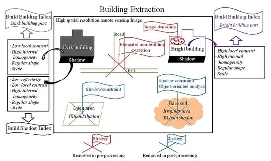
:A new morphological attribute building index (MABI) and shadow index (MASI) are proposed here for automatically extracting building features from very high-resolution (VHR) remote sensing satellite images. By investigating the associated attributes in morphological attribute filters (AFs), the proposed method establishes a relationship between AFs and the characteristics of buildings/shadows in VHR images (e.g., high local contrast, internal homogeneity, shape, and size). In the pre-processing step of the proposed work, attribute filtering was conducted on the original VHR spectral reflectance data to obtain the input, which has a high homogeneity, and to suppress elongated objects (potential non-buildings). Then, the MABI and MASI were calculated by taking the obtained input as a base image. The dark buildings were considered separately in the MABI to reduce the omission of the dark roofs. To better detect buildings from the MABI feature image, an object-oriented analysis and building-shadow concurrence relationships were utilized to further filter out non-building land covers, such as roads and bare ground, that are confused for buildings. Three VHR datasets from two satellite sensors, i.e., Worldview-2 and QuickBird, were tested to determine the detection performance. In view of both the visual inspection and quantitative assessment, the results of the proposed work are superior to recent automatic building index and supervised binary classification approach results.
1. Introduction
Buildings are one of the most important types of artificial targets in the urban environment. Due to the high frequency of changes in buildings, understanding their current distribution is important for urban planning, change detection, urban environmental investigations, and urban monitoring applications [1]. The use of a new generation of very high spatial resolution sensors, such as Ikonos, QuickBird, and Worldview, has broadened the application of remote sensing technology [2]. A great amount of spatial and thematic information on land cover at local and national scales is contained in VHR data [3], and this information clearly gives buildings identifiable shape and texture features. In view of this, VHR images are suitable for building feature extraction tasks. However, the high intra-class variance and the low inter-class variances in the spectral statistics of VHR images greatly reduce the distinguishing ability of small land-cover areas in these images [4]. To address this problem, numerous studies have focused on the extraction of spatial and structural information in images and the use of this information as a supplement to improve the recognition ability [5]. Researchers have indicated that importing spatial features significantly improves the accuracy of VHR image classification [6,7,8]. For building feature extraction applications, current works mainly use supervised machine-learning approaches [9,10,11,12,13]. However, such methods require a large number of training samples and a high time cost in the sample selection stage. In recent years, some automatic building detection methods for high-resolution satellite imagery have been proposed. Different strategies, such as automatic building boundary extraction [14], automatic building feature extraction combined with an existing geodatabase [15], and the use of LiDAR data [16], have been employed in these studies. In addition, a number of building feature indexes have been proposed to characterize potential buildings [17] or exclude confused non-building features, such as vegetation [18], water [19], and shadows [20].
In recent years, a combination of the morphological building index (MBI) [21] with the morphological shadow index (MSI) [22] has been proposed to automatically detect buildings in VHR images. By modeling the local contrast, building-directivity, and granulometry with a series of multiscale morphological profiles (MPs) [23], the MBI and its variants [24,25,26] have proven to be effective tools for building detection tasks. However, MPs do not fully exploit spectral information, which restricts the extraction performance to some extent.
Concerning the above restriction, morphology attribute profiles (APs) [27] are proposed as an extension of MPs. As a more flexible way than MPs to model information from high-resolution images, the transformations in APs can extract features based on either the geometrical or spectral characteristics of objects. According to the different attributes considered in the morphological attribute transformation, different features can be obtained from a VHR image. Classification [28], building feature extraction [29], and change detection task [30] results have suggested that the use of APs is an effective way to model spatial information from VHR images. However, instead of acting as an automatic image-processing index, APs often work as ancillary features of the spectral characteristics in supervised learning. That is, the intrinsic land-cover recognition ability of APs may be underestimated, prompting researchers to continue to study it.
In this paper, a novel morphological attribute building index (MABI), as well as the morphological attribute shadow index (MASI), are proposed, and the study contributions can be summarized as follows:
(1) In the pre-processing step, APs were used to maintain the homogeneity of the original image. In addition, a new strategy to eliminate bright narrow and long non-building artificial objects, such as bright paths, road and narrow open ground, is proposed.
(2) A new building feature index based on APs, the MABI, is proposed for automatic building feature extraction. By the sequential application of attribute filters (AFs), multilevel characterization of the VHR image was obtained to model the structural information of buildings. Considering the different reflectance characteristics of buildings in the VHR image, features of bright buildings and dark buildings were extracted separately in the MABI to reduce the omission rate caused by the absence of dark roofs.
(3) Furthermore, in the post-processing step, the MASI, which is derived from the MABI, is proposed for the automatic shadow detection task. With the aid of the spatial co-occurrence between buildings and shadows, some confused flat features, such as regular bare land and open ground, could be filtered out.
2. Morphological Attribute Building Index
The flowchart of the proposed framework is shown in Figure 1. There are three main parts contained in the proposed framework: pre-processing, building feature extraction, and post-processing. Before jumping into the steps in detail, the APs, the basic mathematical foundation, are presented at first (Section 2.1). The pre-processing step is then presented (Section 2.2). The proposed building and shadow indexes, MABI and MASI, are calculated to obtain the building and shadow features (Section 2.3 and Section 2.4, respectively). To better detect buildings from the obtained feature images, a post-processing framework is designed (SubSection 2.5). The variable notations used in this article are defined in Table 1.
2.1. Attribute Profiles
APs are multi-scale features obtained by conducting the sequential application of AFs. AFs [31] are morphologically connected filters that act on the image by merging the connected components that compose the image according to the filter criterion. The connected components represent the regions that are composed of the spatially connected isointensity pixels in the image. According to the filter criterion of AFs, the transformation evaluates the value measured for each connected component in the image of an arbitrary attribute against a given filter parameter. For example, the filter criterion: means that, given the attribute Attr, the attribute value calculated on the connected component C is compared against the given reference value. The merging rule of AF is as follows: The regions that fulfill the given criterion remain unaltered, while the regions that do not fulfill the criterion are merged with darker or brighter (according to the grayscale value) adjacent regions corresponding to the extensive (i.e., thickening) or anti-extensive (i.e., thinning) transformation, respectively. These two transformations can be further subdivided into increasing (for the increasing criteria, one connected component satisfies the criterion and the subset components also meet this condition) and non-increasing categories according to the attribute selected in the filtering criterion. The non-increasing operation is not uniquely defined when dealing with grayscale images because it obtains different results according to the selected filter criterion [32]. For the non-increasing criterion, the basic operators are thinning and thickening, while the operators for the increasing criterion correspond to opening and closing. As two basic AF operators, multiscale thinning (or opening) and thickening (or closing) transformations can detect dark and bright objects, respectively.
For the grayscale image b, the APs obtained according to a sequence of ordered criteria with m attributes are defined as
where and are the m attribute closing and attribute opening operators according to criterion T, respectively. The EAPs are the extension of the APs in multi-band images. The EAPs obtained from the multi-band image f can be defined as
where bn is the nth band of image f.
Progressive filtering residuals at multiple scales can be used for describing the structural composition of image contents [33]. Each obtained profile is associated with a specific scale. By computing the derivative of the profiles, a differential attribute profile (DAP) generated by an ordered set of criteria is
where and are the differential closing and opening profiles, respectively. To better understanding the multiscale DAP, we took the attribute named the diagonal of the minimum enclosing rectangle (ld), a measure of the object size, as an instance to describe the multiscale approach, where five scales with size T = {10,30,50,70,90}. Given a grayscale image, as shown in Figure 2j, opening profiles on ld at each elements are presented in Figure 2a–e in sequence. Furthermore, the different operation of APs between adjacent scales was computed to capture the components in the range of specific scales. Differences between each profile are shown in Figure 2f–i.
To enhance the efficiency of attribute filtering, an effective data structure named max-tree [34] is used in building APs. The image filtering processing comprises three procedures: First, the image is represented by a hierarchical tree. For the grayscale image, the depth of the tree represents the number of gray levels of the image after threshold decomposition. The number of nodes is associated with the number of connected components of the binary image on the current graylevel. The tree is then pruned by evaluating the reference value at each node. The filtering process is performed by removing the nodes that do not satisfy the filtering criterion. Finally, the pruned tree is converted back into an image. The max-tree is particularly applicable for the computation of multiple filtering, e.g., profiles and granulometries, because the structure completes filtering with different criteria by creating the tree only once. The attribute values are calculated for all regions in the image before the image filtering step, and the filters then prune the tree according to the defined criterion.
In this paper, every EAP feature is calculated using Profattran software, which was kindly provided by the authors of the article [35].
2.2. Pre-Processing
Pre-processing consists of two steps: image denoising and elongated non-building object detection. The entire pre-processing flow chart is shown in Figure 3.
2.2.1. Image Denoising
The diverse materials of building roofs in a VHR image show different reflectivities, while the interior of building rooftops usually presents as a region with high spectral homogeneity. In view of this, the high contrast between the interior homogeneous section and its surroundings is often utilized as a basic principle of morphological operator-based building feature extraction strategies. However, variations in the bright image of VHR, which is calculated as the maximum value of each spectral band and acts as the basic unit for MBI-like processing, may lead to the incomplete extraction of building features. To maintain homogeneity and remove the small amount of dark noise inside bright homogeneous regions, an image denoising process based on AFs is applied to the original spectral reflectance image. This step corresponds to Box ① in Figure 3.
The standard deviation of the pixels belonging to each region (denoted by sd) is chosen as the filtering attribute in the image denoising task. This attribute is used to measure the spectral homogeneity of the intensity values of the pixels in the region. Equation (1) shows that APs are generated by a sequence of closing and opening profiles. For the APs built on a region (a set of pixels treated as a basic unit of the filters), all pixels in the region are located in either the closing or opening profiles. In fact, dark regions are obtained in the closing profiles and bright regions are obtained in the opening profiles. To keep the bright homogeneous regions and remove the small amount of dark noise, the opening operator is employed. Since sd is a non-increasing attribute, the opening operator corresponding to sd is attribute thinning. The stack of thinning profiles built on sd by the criterion from the multispectral image f is obtained according to Equation (2). The maximum value of corresponding pixels in each obtained thinning profiles is then calculated, denoted by . After image denoising, bright regions with high homogeneity in the original image remain in the maximum result, and the small dark structures are filtered out. It should be noted that AFs only process the image by suppressing the regions that do not meet the criterion without edge blur. With the virtue of maintaining edges for following building geometrical characteristic descriptions, AF is an effective tool, as a pre-processing step following building detection. By calculating the maximum values of each profile, the obtained regions with high reflectivity and homogeneity correspond to potential buildings.
2.2.2. Elongated Non-Building Object Detection
Buildings in dense urban areas are often easily confused with adjacent non-building landcovers, such as open parking lots, bare soil, roads, and small paths. This confusion is mostly attributed to the similar spectral characteristics of these land covers to buildings in the VHR image. Since these non-building land-covers may result in false alarms in the building feature extraction results, it is necessary to identify them independently. By analyzing the shape characteristics of roads and open areas surrounding buildings, it was found that these features generally present as elongated and curve-shaped regions. In this study, these objects are named elongated non-building objects. The elongated non-building object detection strategy is shown in Box ② of Figure 3 and is divided into two steps: a) elongated feature extraction and b) elongated feature segmentation.
(a) Elongated Feature Extraction
Despite the varying shape of buildings, the compactness of buildings is generally higher than that of roads and paths. Therefore, the attribute that measures the compactness of objects is considered able to separate building and non-building objects. In this part of the paper, a geometric attribute, i.e., the first moment invariant of Hu [36], denoted by Hu, is considered the filter attribute in the attribute filters. This attribute describes the ductility of a region relative to its centroid, which indicates the degree of non-compactness of an object, and the indexes in Hu are invariant to translation, rotation, and scaling [37]. The value of Hu is small for the compact region and gradually increases for the elongated regions. Since Hu is a non-increasing attribute, the thinning profiles filtered by Hu are used to detect bright and elongated non-building objects.
The elongated feature is calculated by the following steps: First, the stack of the thinning profiles is obtained by conducting a thinning operation on each profile in , which is obtained in the previous image denoising step, with attribute Hu according to criterion λHu. To detect structures with a high reflectance, the maximum of the profiles obtained in the first step is then calculated and acts as the input in the next segmentation step.
(b) Elongated Feature Segmentation
Since buildings also show elongated shape characteristics to some extent, object-oriented analysis is carried out to prevent potential buildings from being missed. Meanshift [38] segmentation is employed to obtain the image objects. To better identify buildings from the other landcovers, an over-segmentation strategy is preferred here. Because the main difference between building and non-building objects in the elongated feature image lies in the different degree of the object that approximates to the rectangle, the rectangular fit (RcFit), which is calculated by the ratio of the area of the object to the area of the smallest circumscribed rectangle of the object, is employed to filter out potential building objects. Objects with a high RcFit value are more likely than objects with a low RcFit value to be buildings. Giving the threshold , the objects satisfying are reserved to compose the resulting map.
Finally, by removing the obtained objects in Box ② from the result in Box ① (shown as Step ③ in Figure 3), a new basic image, denoted as I, is obtained. I acts as the input image in the following building feature extraction steps.
2.3. Morphological Attribute Building Index
Since buildings in high-resolution images are variable in size and orientation, a multiscale strategy is performed in the building detection task. Considering the regular shape of buildings, the length of the diagonal of the minimum enclosing rectangle, referred to as ld, is used to measure the scale characteristic of the objects. Both the attribute area and ld in attribute filtering can be used to measure the scale of objects. The ld rather than the area is chosen because attribute opening using ld retains more grain boundary segments than that using area [31]. In addition, the rectangular shape of buildings makes ld more suitable than area to measure the scale characteristics in the building detection task. The DAP can be built with an increasing criterion of attribute ld to obtain scale information.
In a VHR image, building roofs can be divided into two parts according to the difference in their spectral contrast with surrounding regions: local bright buildings and local dark buildings. To reduce the omission rate caused by dark roofs, these two types of buildings are detected separately in the MABI. The bright and dark building features in the MABI are recorded as MABIbright and MABIdark, respectively.
The procedures for calculating MABIbright from I are as follows. Since ld is an increasing attribute, the opening profiles obtained from I by attribute ld according to criterion t is denoted by . Considering the complex spatial patterns of the building, granulometry is conducted by building the DAP of the opening profiles obtained by attribute ld with an ordered set of criteria , and the MABIbright is calculated as
where is the interval of threshold T, and max represents the max value of the corresponding pixels in all profiles. Through the above steps, the spectral characteristics (homogeneity and contrast) and spatial characteristics (size and shape) are addressed.
The procedures presented above are straightforwardly extended to MABIdark by replacing the opening profiles with closing in Equation (4), and the MABIdark is calculated as
Since shadows also present as relatively dark regions in VHR images, some shadows may be contained in MABIdark. To remove potential shadows, the spectral value of the pixels in the original image is considered. Because of the low reflectivity of the shadow in each visible band of the original image, the bright image is calculated by the max value of the pixels in all visible bands. The pixels in MABIdark that satisfy are saved as MABIdark. With regard to the characteristics of buildings as homogeneous and continuous areas, pixels with high MABI values are more likely than those with low MABI values to be buildings.
2.4. Morphological Attribute Shadow Index
The spectral and geometrical characteristics of shadows are opposite and similar, respectively, to the corresponding characteristics of adjacent buildings. A shadow presents as a homogeneous dark area with geometrical characteristics similar to those of the adjacent building. Considering the high homogeneity, low spectral reflectance, and shape characteristics of shadows, the procedures for building the MASI are similar to those for building the MABIdark to obtain the dark structures in I. Furthermore, considering the different scale characteristics between buildings and shadows in the satellite image, the threshold value of ld in shadow detection is smaller than that in dark building feature extraction.
Due to the low spectral reflectance of shadows, the MASI is calculated by transforming the max operator in Equation (5) into the average value of the DAP feature:
The pixels with large values are more likely than those with small values to be shadows in the MASI. Finally, the pixels that satisfy the conditions , , and are treated as shadows, where , indicate the threshold of the vegetation index (NDVI) and the MASI, respectively. The threshold of brightness is used to remove structures that have a high reflectance but are darker than the surrounding structures.
2.5. Building Extraction Framework of the Proposed Method
Extracting buildings by the dual threshold segmentation of the MABI may cause high commission errors (CEs) and omission errors (OEs). The CEs mainly come from the land covers that have similar characteristics with buildings, such as bare soil and roads, while the OEs are often related to dark roofs. To address these problems, a building feature extraction framework is conducted via the following steps.
First, the MABIbright image is divided into two parts: Given a threshold TMABI, the high-MABI and low-MABI regions are separated. Pixels that satisfy the TMABI in each part are assigned a value of one, and other pixels are assigned a value of zero. Object-oriented analysis can be performed on the obtained binary image. The objects belonging to the high-MABI region are analyzed with a relatively low shape threshold to prevent the bright irregular buildings from being missed, while objects in the low-MABI and MABIdark regions are analyzed by more strict geometric constraints. The RcFit and shape index (SI) values are utilized to measure the shape characteristics of objects. The SI is calculated by the boundary length of an object divided by four times the square root of its area. SI measures the smoothness of the object boundary, and more fragmented objects tend to have a high SI value.
According to [22], the distance between shadows and buildings is considered to suppress non-building objects. Different distance thresholds are set to objects in the high-MABI and low-MABIcategories, respectively. The thresholds on MABIdark are the same as the low-MABI thresholds. To present the entire processing flow more intuitively, a small region acting as an instance is shown in Figure 4.
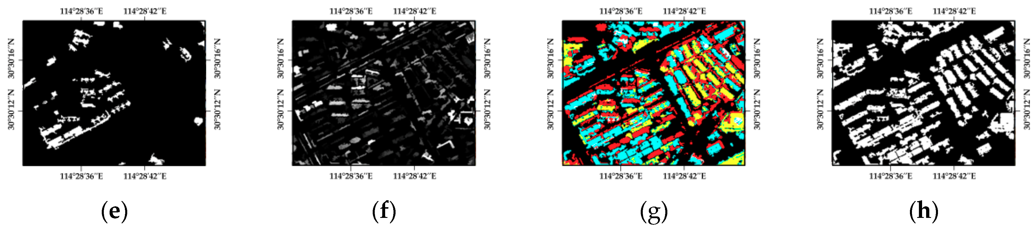
Bright bare soil, roads, and small paths are easily confused with buildings. Figure 4b,c are images resulting from the two steps in the pre-processing step, respectively. (b) is the image obtained after image denoising, and (c) is the input image I. The two images show that, although the bright roads at the top of the image have spectral properties similar to those of the surrounding buildings, these roads and buildings are separated by their different shape characteristics in the elongated object detection step. After removing non-building objects, the false alarms in the input image I are reduced; for example, the bright open ground and small paths in the top left corner of (b) are removed in (c). The building maps obtained from MABIbright and MABIdark are presented in (d) and (e), and the MASI feature image is displayed in (f). The parameter setting in this dataset is the same as the datasets in the experiment section. A detailed analysis is provided in the following parameter analysis section. (g) is the overlapping image of the buildings and shadows obtained by the proposed method. Buildings in the high-MABI part are colored in yellow, and the low-MABI and MABIdark parts are colored in blue; shadows are colored in red. The building feature extraction result obtained by measuring the distance between the shadows and buildings is shown in (h). (h) shows that the buildings are retained and backgrounds are removed in comparison with (g).
3. Building Feature Extraction Experiments
3.1. Datasets and Experimental Strategy
3.1.1. Dataset Description
The proposed building feature extraction framework was applied to three high-resolution remote sensing images, which are radiometrically and geometrically calibrated in this section. These VHR images and the corresponding reference images are displayed in Figure 5. The ground truth images were manually delineated by field investigation and visual interpretation. Some representative subgraphs, which are marked with red (Images I1, I3, and I5) and blue (Images I2, I4, and I6) rectangular boxes in Figure 5, were chosen for detailed comparison and analysis. The basic information of the three datasets is listed in Table 2.
3.1.2. Experimental Set-Up
A comparative study between the MABI and MBI was performed to investigate the effectiveness of the proposed method. The recommended values in [22] were selected as the thresholds for the MBI. To obtain a fair comparison result, the same NDVI threshold and object-oriented analysis processes were conducted on both the MABI and MBI. The effectiveness of the pre-processing and shadow verification step in the proposed framework was explored by comparing the results obtained by the MABI and MBI under different conditions.
To further verify the effectiveness of the proposed algorithm, two widely used classifiers including support vector machines (SVM) [39] and random forest (RF) [40] were also used for comparison. In addition to the original spectral information of the image, there are two spatial characteristics used for classification in the above two supervised classifiers. The first comprises the multiscale and multidirectional DMPs that are used to compute the MBI. By feeding spectral bands and the DMPs into the SVM and RF, the binary classifiers DMP-SVM [41] and DMP-RF divide the test image into buildings and non-buildings. The second is the object-oriented SVM and the object-oriented RF. Employing object-based methods on VHR images can generate spectral and shape information to improve the accuracy of building feature extraction. In this study, the meanshift algorithm was used for segmentation. The spectral features of the object employed in the object-oriented SVM were the brightness and the spectral standard deviation of the object, and the spatial features were the length–width ratio, area, border length, RcFit, and SI. The parameters for the SVM and RF were set according to specific suggestions [39,40]. The number of training and test samples used in the supervised classification algorithms of each dataset is reported in Table 3. In this study, an SVM, which was implemented with the help of the LibSVM package, was used as a supervised binary classification to label each pixel in a high spatial resolution image as building/non-building (i.e., background). The nonlinear SVM with radial basis kernel was used and is abbreviated as SVM in the revised manuscript. All parameters in this SVM were tuned by five-fold cross validation. Except for the SVM-related work, which was implemented with the help of the LibSVM package using C++, processes were performed using MATLAB R2014a on a computer with a single i5-24003.10 GHz processer and 8.0 Gb of RAM.
The parameters used in the proposed method and their suggested range are summarized in Table 4. The parameter sensitivity is further analyzed in the discussion section, and several issues should be noted. First, appropriate ranges of parameters for the proposed framework were analyzed in this study. Second, most of the parameters could be kept the same for different datasets, and the parameters were fixed for all three datasets in this paper. The accuracy statistics were calculated according to the correctly classified pixels in the building feature extraction map of each method. The building detection accuracy was evaluated by the following four statistical measures: overall accuracy (OA), Kappa coefficient (Kc), omission errors (OEs), and omission errors (CEs) [42]. The first two indexes were computed based on the confusion matrix [43], and the remaining two indexes measure the accuracies of classification.
3.2. Experimental Results
3.2.1. General Results and Analysis of the Datasets
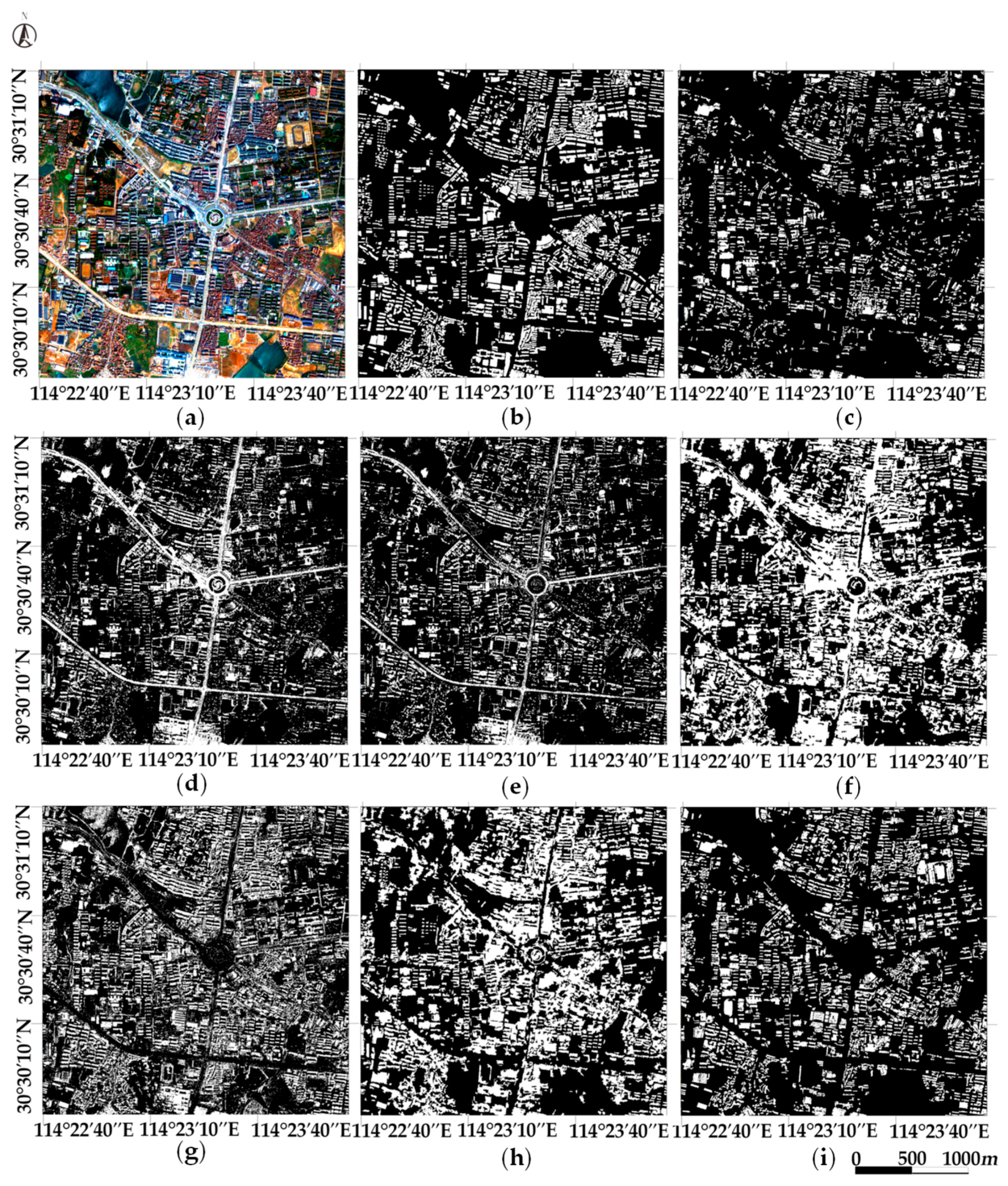
The building detection results of the three datasets are given in Figure 6, Figure 7 and Figure 8, respectively, in which the detected buildings are in white pixels, and the background is in black pixels. Three datasets of urban areas have their own characteristics. There is a dense road network in Dataset 1. The difficulty of this dataset lies in the similarity between the spectral characteristics of roads and buildings. Compared with the buildings in Dataset 1, Dataset 2 has a high-density urban area. The varying spectral characteristics of building roofs and the existence of certain building groups increase the difficulty of analyzing Dataset 2. To carry out a comprehensive experiment, an image containing a large number of non-buildings was chosen as Dataset 3. This image has a large area of bare ground and vegetation, which poses a challenge to the building feature extraction task.
The quantitative results of the different algorithms are reported in Table 5. The statistical accuracy and the visual inspection ((d) in Figure 6, Figure 7 and Figure 8) show that the pixel-based SVM leads to unreliable results in the three datasets. This inferior performance is mainly due to the poor discriminatory ability of using only the spectral value of the original image. By joining the spatial information, the remaining algorithms obtain more acceptable results according to the statistical values in Table 5. Furthermore, in most cases, the proposed framework obtains competitive results. Detailed analysis of the results of the MBI, DMP-SVM, DMP-RF, object-oriented SVM, object-oriented RF, and the proposed method are as follows.
The MBI performed well for all three datasets. The OA of the MBI was second only to that of the proposed method in most cases, according to Table 5. Compared to the MBI OA, the OA of the proposed method increased by 1.46%, 2.97%, and 1.53% for the three datasets. The Kappa coefficient, increased from 0.62, 0.61, and 0.66 to 0.69, 0.68, and 0.7, respectively. The MBI was subject to a high CE rate in Datasets 1 and 3 due to the misclassification of non-buildings in the scenes. Regarding both the OE and CE, the proposed method obtainedbetter results than the MBI. For example, the OE and CE decreased by 23.04% and 5.44%, respectively, in Dataset 1 and by 8.74% and 5.44%, respectively, in Dataset 3. The improvement of the CE in the proposed framework can be ascribed to the removal of non-buildings in the input image. In Datasets 1 and 3, there were many building blocks that were darker than the surrounding backgrounds. These buildings were excluded from the MBI results, causing the increase in the OE. The proposed MABI compensated for the missing buildings by a separate consideration of dark buildings.
The analysis of the outcomes of the DMP-SVM, DMP-RF, object-oriented SVM, and object-oriented RF demonstrates that, with the introduction of supervised machine learning, the two algorithms obtained competitive results. In particular, the OA of the two object-oriented methods for Datasets 1 and 3 is comparable to that ofthe proposed framework. Table 5 shows that the object-oriented SVM and RF obtained the lowest OE but were subject to severe omission problems. This problem wasparticularly noticeable in the dense building area in Dataset 2. A large area of asphalt roads that have similar spectral characteristics as the buildings in Datasets 1 and 3 caused an increase in false alarms in the results of the object-oriented classifiers. Although the object-oriented methods increased the efficiency and identification ability of the supervised classifier, the accuracy was dependent on the choice of representative training samples. The same problem also existed in the DMP- SVM and DMP-RF. The OA of these two methods in Dataset 2was obvious lower than that in Datasets 1 and 3. However, from the result in Datasets 1 and 3, it was found that the discrimination power of the SVM was obviously increased by feeding the multi-scales and the multidirectional DMP feature. Compared with the pixel-based SVM that used only the spectral features of the image, the OA significantly increased in the three datasets. Nevertheless, supervised classification algorithms are time-consuming. An analysis of the above experiment results shows that the proposed MABI is more suitable than the other methods for the feature extraction of buildings in large and complex urban areas.
The running times of the different algorithms are reported in Table 6. The pixel-based SVM and MBI were the most efficient, followed by the proposed method. The other supervised methods still had a much higher cost than these two unsupervised ones, except for the cost of the training sample collection. Regarding the two unsupervised methods, in view of the detection superiority of the proposed work over MBI, it was considered that the proposed one is generally preferable.
3.2.2. Visual Comparisons of the Representative Patches
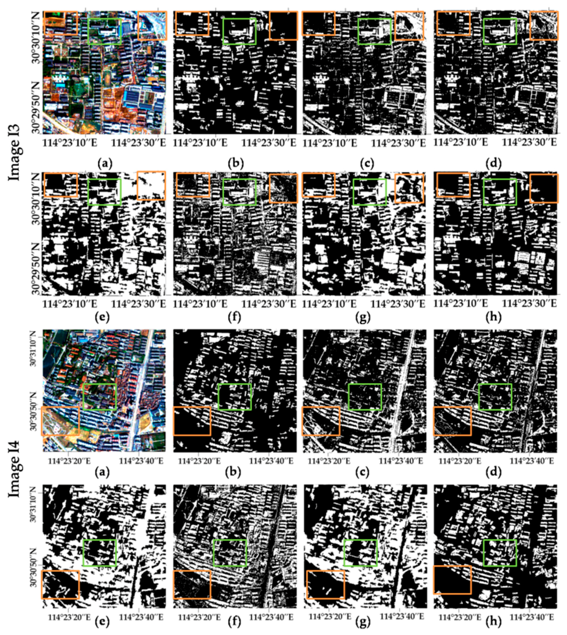
The results of the representative patches in each test image are reported in Figure 9 (show Images I1 and I2), Figure 10 (show Images I3 and I4), and Figure 11 (show Images I5 and I6), respectively. The results obtained by the proposed framework are the most complete and precise in most scenes. The object-oriented SVM was subject to false alarms in the dense urban area, and the DMP-SVM was affected by the omission phenomenon, especially for heterogeneous buildings. The results of each representative patch are discussed as follows.
The buildings in I1 and I2 in Figure 9 are surrounded by vegetation and bare soil. All detectors filtered out most of the vegetation, but, except for the proposed method, some bare soil and open ground information (yellow rectangles in I1 and I2) was incorrectly extracted. Some buildings with poor internal homogeneity (green rectangles in I1) were excluded by the MBI and DMP-SVM. The two object-oriented classifiers and the proposed MABI correctly extracted these building features by increasing the internal homogeneity of image objects before the building feature extraction step via segmentation and the proposed image denoising step, respectively. Patches I3 and I4 in Figure 10 show dense building areas, and the paths adjacent to buildings (green rectangle in I3 and yellow rectangle in I6 in Figure 11) were detected as buildings in the MBI and all supervised methods. As for the proposed framework, the paths were detected and removed in the pre-processing step. The bare ground (yellow rectangle in I3 and I4 in Figure 10), which was well removed with the constraint of shadows in both the MBI and the proposed method, was wrongly identified by all supervised methods. In the green rectangle in I4, the similarity between the spectral characteristics of buildings and the surrounding backgrounds made it difficult to identify buildings while excluding the backgrounds. A large number of buildings in this region were missed in most result maps, but the proposed method still identified the highest number of correct buildings. Patch I5 in Figure 11 shows a building block with low reflectivity and internal homogeneity. The heterogeneity of building roofs led to some omission phenomena in the results of the MBI and DMP-SVM. The DMP-SVM and object-oriented RF extracted the building features completely, but was still subject to under- and overestimation, respectively. The false alarms, such as the roads with spectral characteristics similar to those of the surrounding buildings were extracted in the object-oriented RF. Because the attribute filtering in the proposed method smooths the image while keeping the original boundaries, the buildings in the results of the proposed method had a more precise outline than those in the object-oriented RF. In summary, the results of these representative patches show that the proposed framework obtains better results than the comparison algorithms in different types of scenes.
4. Discussion
In this section, we first discuss the role of each step of the proposed method and then conduct parameter sensitivity analysis to verify the relative robustness of the proposed method.
4.1. Step Analysis of the Proposed Work
4.1.1. Effects of Denoising in Preprocessing: Analysis on MBI and MABI
To show the efficiencyof image denoising in the pre-processing step, denoting the image obtained after image denoising step as I’, the MBI and MABI features were calculated based on the bright image (marked as MBI and MABI (bright) in Figure 12) and I’ (marked as MBI(I’) and MABI in Figure 12). Each statistical result table in Figure 12a–c is composed of 320,000 randomly selected pixels from all datasets. The diagram displays the classification accuracy of the building and background areas in MBI, MABI (bright), MBI(I’), and MABI. To ensure a fair comparison, the MABI feature considered here is the high-MABI part calculated by the application of binary segmentation on the MABI according to the TMABI given in Table 4. The thresholds in the MBI are set according to values suggested in [21]. The classification accuracy is a statistic from the results without the shadow constraint.
As shown in Figure 12, both the MBI and MABI can extract most of the building features from the bright image and I’, respectively, but the proposed method extracts the most accurate building information while filtering out false alarms. The OA of the buildings in the three tables is slightly improved from left to right. Specifically, after replacing the input image from the bright image to I’, the increase in the OA of the MBI is more obvious than that of the MABI in tables (a) and (c). Due to the improvement in both the MBI and MABI, I’ is more suitable than the bright image as the input image for building feature extraction. Furthermore, the observable increase in the correct backgrounds in the results based on I’ also shows the good effect of I’ on suppressing background noise in the building detection task.
A representative patch I5 is chosen for further comparisons. Again, the results displayed in Figure 13 confirm that using I’ as the input image can effectively suppress false alarms in the building feature extraction results. For example, the highlighted vegetation and inhomogeneous bare land in the green box and the roads in the yellow box were removed by changing the input image from a bright image to I’. The improvement in the building feature extraction accuracy is attributed to the increase in the homogeneity of image I’; in addition, both statistical tables and images show that the MABI obtained a more accurate result than the MBI under identical conditions. For both the bright image and I’, the proposed MABI achieves more accurate results than the MBI, and the most appropriate combination is the proposed one.
4.1.2. Functions of Elongated Non-Building Object Detection and Dark Building Feature Extraction
The first step was utilized to reduce the non-building objects in the input image I before building feature extraction. The dark building feature extraction step was conducted to account for missing dark roofs. To illustrate the role of these two processes, the quantitativeresults for each step of the three datasets in Table 7 and three patches of a dense urban area in Figure 14 were utilized for statistical and visual comparisons, respectively.
The values in Line 2 of the MABIbright of the proposed methodhavean obviously lower CE compared with the results of the MABIbright feature without eliminating the elongated objects for the three datasets. This improvement reflects that removing easily confused non-building objects in the input image can effectively reduce the false alarms in the final result. The red regions in Figure 14b show that the regular road in I3, the open ground in I4, and the small paths in I5 are filtered out in (c). This improvement demonstrates that detecting these objects is necessary to reduce false alarms that cannot be recognized in post-processing. Line 3 of Table 7 represents the accuracy of the MABI that combines the results of MABIbright and MABIdark before shadow constraint. For Datasets 1 and 2, the four MABI statistics are better than the results in Line 2. As for Dataset 3, due to the large area of dark backgrounds, the CE in Line 3 is slightly increased compared to that in Line 2 after the feature extraction of dark buildings, which also led to a slight decrease in the OA. Nevertheless, the decrease in the OE of Dataset 3 was the largest of the three data sets. This result can be viewed visually in Patch I5 of Figure 14. The missing buildings in the green region in (c) were supplemented in (d). Moreover, a slight increase in the CE is acceptable when compared with a substantial decrease in the OE, and false alarms can be further removed with the shadow constraint.
4.1.3. The Usage of Proposed Shadow Detection: Analysis on MSI and MASI
Shadow constraint was used to filter out the non-buildings from the obtained building map in the post-processing step. Since the omission of shadow should lead to an increase in the OE value, and the false-positive shadows may cause an increase in the CE value, the accuracy of four results from a pairwise combination of two shadow detection and two building feature extraction results (MBI and MABI) are given in Table 8 to compare the shadow detection results of the MSI and the proposed MASI. Lines 1 and 2 in Table 8 are the building detection results of the MBI with the shadow constraints of the MSI and MASI, respectively. Line 3 lists the building detection results of the MABI with the shadow results of the MSI. The combination of building maps with the proposed MASI (in Lines 2 and 4) obtained a higher OA than that with MSI (in Lines 1 and 3) for the three datasets. The reduction in CE and OE values also proves the effectiveness of the MASI. The comparison of these results shows that the most accurate combination is the proposed work.
4.2. Parameter Analysis
In this section, the values of some important parameters of the proposed method are discussed.
4.2.1. Pre-Processing Parameters
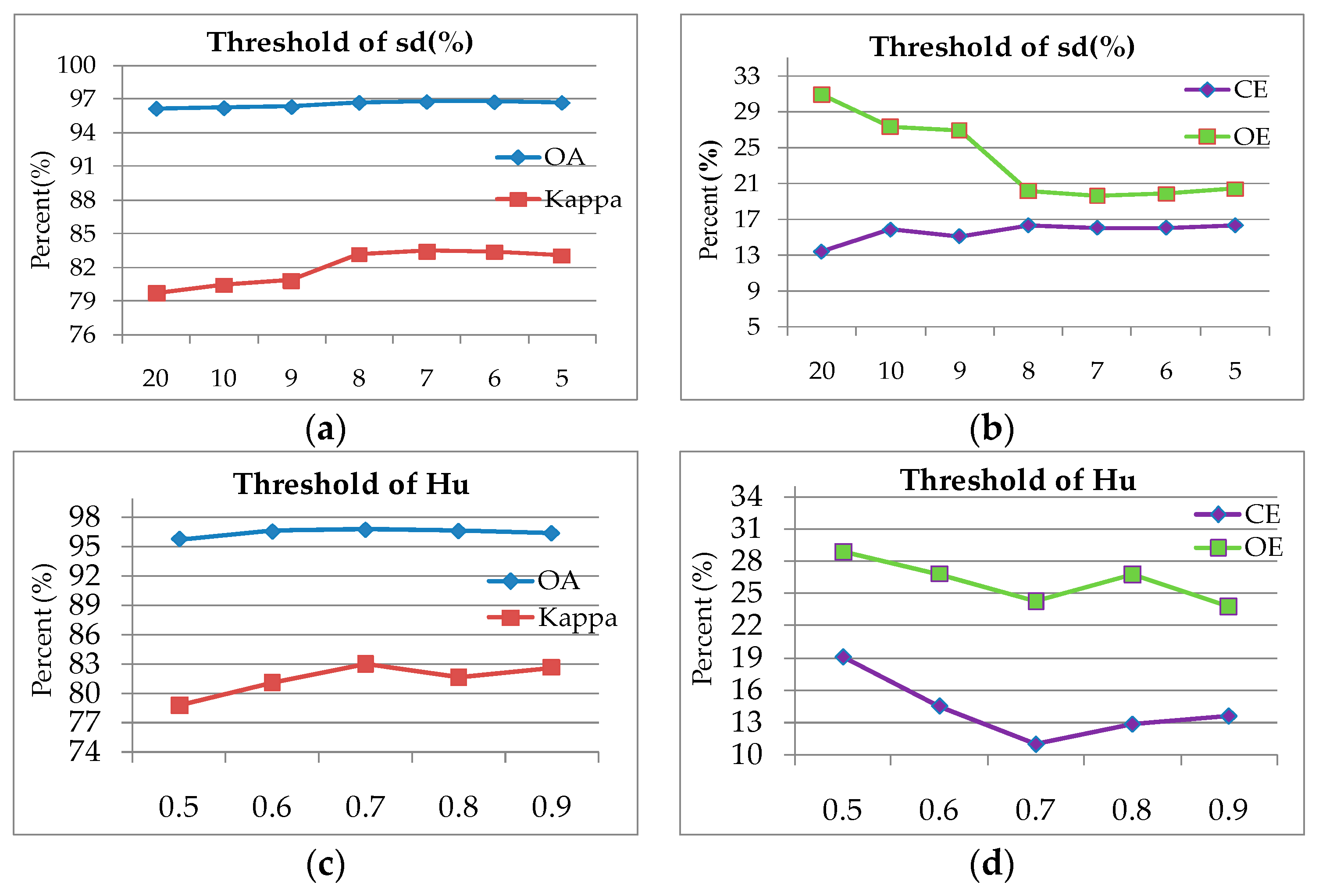
The thresholds for the attributes sd and Hu used in the pre-processing step are analyzed here. Attribute sd was employed to increase the homogeneity of the original image. A high value of sd corresponds to a high object homogeneity. Analyzing the gray histogram of the filtering results with different thresholds shows that, when the threshold value is greater than 20, most objects in the complex urban image are removed after filtering, and the effect of the AF is not obvious when the threshold is below 5. Therefore, the threshold values in [5,20] are discussed here. Figure 15a,b show the relationship between the value of sd and the building feature extraction precision of Dataset 2. The OE and CE are more balanced when the threshold is between 5 and 8, and a satisfactory and stable OA and Kappa coefficient rate are also obtained in this interval. When the proposed framework was applied to images with a high, medium, and low building density, the threshold value of sd in [5,8] possessed good generality and stability for the different scenes. Furthermore, a relatively small threshold is recommended for dense building areas, and a relatively large threshold can be selected for images containing a high amount of background. The suggested threshold for attribute sd in shadow detection is the same as that of the parameters in building feature extraction since shadows and the surrounding buildings have similar characteristics.
The Hu attribute was used to detect the elongated non-building objects in the pre-processing step. Hu indicates the non-compactness degree of the objects and ranges from 0 to 1. The value is gradually increased from compact to elongated objects. Since buildings are compact objects in the image, a small value of Hu can filter out some buildings, so Hu values below 0.5 are not considered here. Figure 15c,d show the relationship between the accuracies of building detection and the threshold value of Hu at [0.5,0.9] of Dataset 2. The four statistical values show an improvement as the value of Hu increases from 0.7 to 0.9. In general, when the threshold is in the interval of 0.7–0.9, the proposed framework achieves a more accurate result. Since Hu is only related to the geometrical characteristics of objects, the thresholds can be safely applied to different images.
4.2.2. Parameters in the Building Feature Extraction Steps
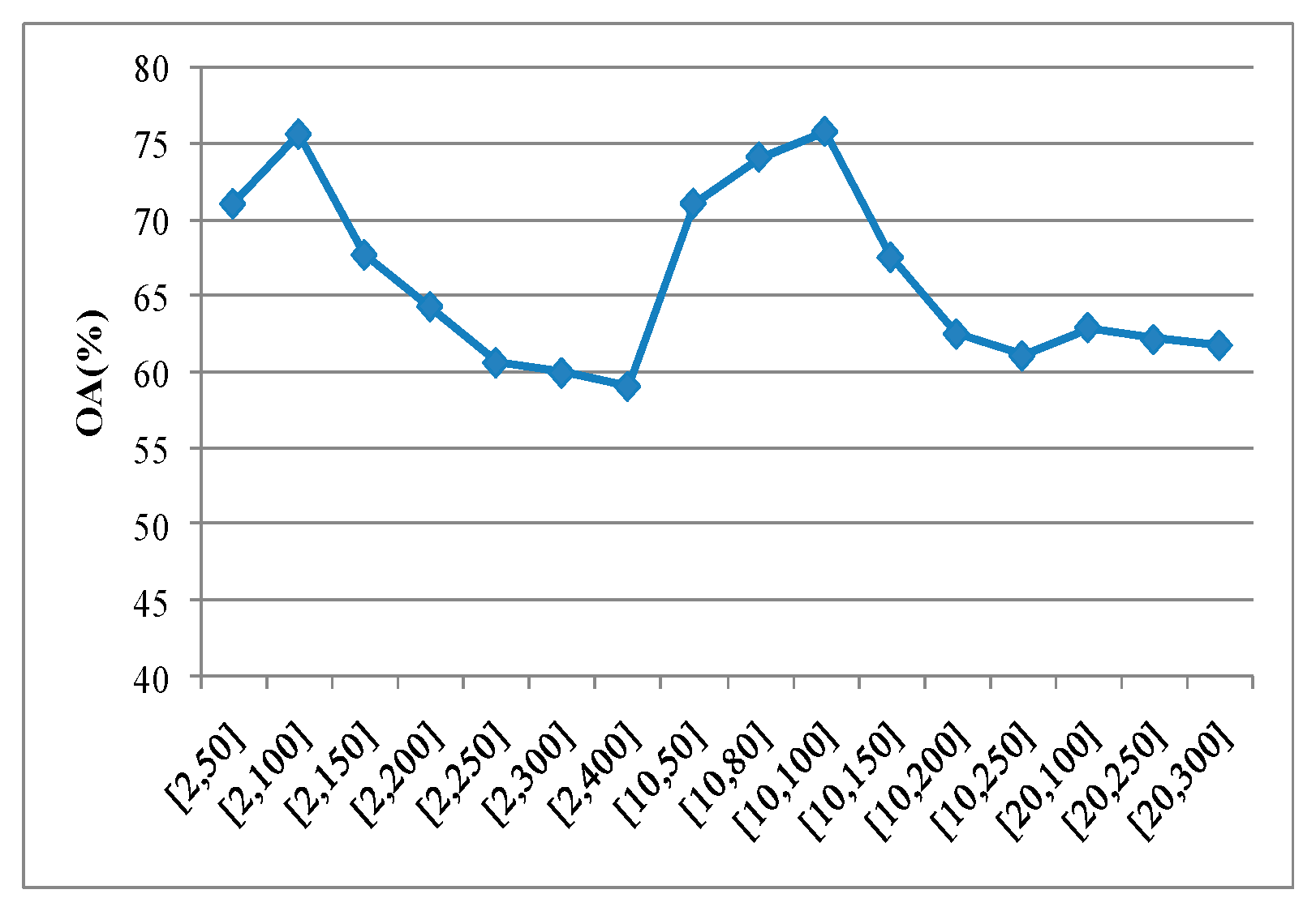
Threshold values of attribute ld in the MABI were arbitrarily selected in terms of the scale of the buildings. The OA of the building detection results (calculated from the MABIbright) of Dataset 2 obtained by different intervals of ld is visualized in Figure 16. The vertical axis represents the OA values, and the horizontal axis represents the ld intervals. ld intervals less than 10 are 2,6,10, with a step of 5 after 10. The OA is obviously decreased after the upper limit of ld exceeds 200 and the minimum lower limit is 20. The accuracies decrease slowly when the upper limit of ld is in the interval [100,200]. According to Equation (4), the value of ld is selected based on the building scale; therefore, an ld value in the interval of [2,100] is suggested for the VHR image of the urban area.
In the proposed framework, many non-building objects are removed in the pre-processing step, so a small threshold value of the high and low MABI is recommended to prevent the removal of some dark roofs. As the MABI ranges from 0 to 1, the suggested threshold is within the range of 0.1–0.4, where the quality scores are stable.
For the threshold value of the distance between buildings and shadows, the NDVI, building area, and SI have been discussed in detail in [22]. The value of the RcFit ranges from 0 to 1, and the larger the value, the more the object approximates the rectangle. For objects in the high MABI region, the RcFit value is between 0.5 and 0.6, while the RcFit value for objects in the low MABI region is between 0.6 and 0.7.
5. Conclusions
In this paper, a new building index, i.e., the MABI, and a new shadow index, i.e., the MASI, are proposed based on morphological attribute operators. An analysis of the existing MBI showed that the building feature extraction algorithm based on morphological operators is subject to some OEs and CEs. The OEs occur when the extraction misses some dark roofs and due to noise in building objects, and the CEs are caused by certain types of land cover, such as roads, bare ground, and open ground, which have spectral and shape characteristics similar to those of buildings. Our work aimed at improving these issues, and the contributions of this study are as follows: First, a thinning operator based on the attribute standard deviation was conducted to increase the homogeneity of the original image. Then, elongated non-building objects were detected to decrease the effect of interference objects in the input image before the building detection process. In the building feature extraction step, dark buildings were considered independently with the MABI to further reduce the OE. By jointly using the MABI and MASI in an object-oriented framework, false alarms were further reduced.
The proposed method was conducted on three VHR images. A comparison of the building detection results of the proposed framework with those of the MBI, DMP-SVM, pixel- and object-based SVM, DMP-RF, and object-oriented RF shows that the proposed method is the most effective at increasing the OA and reducing the OE and CE, especially for images with few buildings and large path and bare ground areas. The parameters of the proposed framework were analyzed, and the threshold selection conclusions can be summarized as follows: sd is used to remove small dark structures and to increase the homogeneity of an image. To maintain the details in the image, the choice of a small threshold is recommended, especially for dense urban areas. The attribute Hu is employed to measure the elongated degree of objects; therefore, a large value of Hu is recommended to better indicate non-building objects. The MABI threshold was used to distinguish buildings from other land cover types. Since a large number of easily confused objects were removed in the pre-processing step in the proposed framework, a small threshold value is recommended to avoid the erroneous removal of buildings.
In future studies, more attributes will be considered to better model the spectral and structural information of scenes for building feature extraction tasks, and automatic threshold selection research is also planned.
Author Contributions
W.M., Y.W. and J.L. conceived and conducted the experiments, and performed the data analysis; S.Z. and M.W. provided advice and helped with the revision of the manuscript. W.M. wrote the article.
Funding
The research was supported by the National Key R & D Program under Grant 2018YFD1100405, the National Natural Science Foundation of China under Grant 41701382, and the Hubei Provincial Natural Science Foundation Project under Grant 220100039.
Acknowledgments
The authors are very grateful for the Profattran software, which was kindly provided by Marpu, et al. (the authors of article [35]).
Conflicts of Interest
The authors declare no conflict of interest.
References
- Pesaresi, M.; Guo, H.; Blaes, X.; Ehrlich, D.; Ferri, S.; Gueguen, L.; Halkia, M.; Kauffmann, M.; Kemper, T.; Lu, L. A Global Human Settlement Layer From Optical HR/VHR RS Data: Concept and First Results. IEEE J. Sel. Top. Appl. Earth Obs. Remote Sens. 2013, 6, 2102–2131. [Google Scholar] [CrossRef]
- Gamba, P.; Dell’Acqua, F.; Stasolla, M.; Trianni, G.; Lisini, G. Limits and Challenges of Optical Very-High-Spatial-Resolution Satellite Remote Sensing for Urban Applications. In Urban Remote Sensing: Monitoring, Synthesis and Modeling in the Urban Environment; John Wiley & Sons, Ltd.: Hoboken, NJ, USA, 2011; pp. 35–48. [Google Scholar]
- Aplin, P.; Atkinson, P.M.; Curran, P.J. Fine spatial resolution satellite sensors for the next decade. Int. Remote Sens. 1997, 18, 3873–3881. [Google Scholar] [CrossRef]
- Bruzzone, L.; Carlin, L. A Multilevel Context-Based System for Classification of Very High Spatial Resolution Images. IEEE Trans. Geosci. Remote Sens. 2006, 44, 2587–2600. [Google Scholar] [CrossRef]
- Huang, X.; Zhang, L. An SVM Ensemble Approach Combining Spectral, Structural, and Semantic Features for the Classification of High-Resolution Remotely Sensed Imagery. IEEE Trans. Geosci. Remote Sens. 2013, 51, 257–272. [Google Scholar] [CrossRef]
- Johnson, B.; Xie, Z. Classifying a high resolution image of an urban area using super-object information. ISPRS J. Photogramm. Remote Sens. 2013, 83, 40–49. [Google Scholar] [CrossRef]
- Yan, W.Y.; Shaker, A.; Zou, W. Panchromatic IKONOS Image Classification using Wavelet Based Features. In Proceedings of the 2009 IEEE Toronto International Conference Science and Technology for Humanity (TIC-STH), Toronto, ON, Canada, 26–27 September 2009; pp. 456–461. [Google Scholar]
- Kuffer, M.; Barrosb, J. Urban Morphology of Unplanned Settlements: The Use of Spatial Metrics in VHR Remotely Sensed Images. Procedia Environ. Sci. 2011, 7, 152–157. [Google Scholar] [CrossRef]
- Pesaresi, M.; Benediktsson, J.A. A new approach for the morphological segmentation of high-resolution satellite imagery. IEEE Trans. Geosci. Remote Sens. 2001, 39, 309–320. [Google Scholar] [CrossRef]
- Bian, L. Retrieving Urban Objects Using a Wavelet Transform Approach. Photogramm. Eng. Remote Sens. 2003, 69, 133–141. [Google Scholar] [CrossRef]
- Huang, X.; Zhang, L.; Li, P. Classification and Extraction of Spatial Features in Urban Areas Using High-Resolution Multispectral Imagery. IEEE Geosci. Remote Sens. Lett. 2007, 4, 260–264. [Google Scholar] [CrossRef]
- Vakalopoulou, M.; Karantzalos, K.; Komodakis, N.; Paragios, N. Building Detection in Very High Resolution Multispectral Data with Deep Learning Features. In Proceedings of the 2015 IEEE International Geoscience and Remote Sensing Symposium (IGARSS), Milan, Italy, 26–31 July 2015; pp. 1873–1876. [Google Scholar]
- Zhang, Y. Optimisation of building detection in satellite images by combining multispectral classification and texture filtering. ISPRS J. Photogramm. Remote Sens. 1999, 54, 50–60. [Google Scholar] [CrossRef]
- Ahmadi, S.; Zoej, M.J.V.; Ebadi, H.; Moghaddam, H.A.; Mohammadzadeh, A. Automatic urban building boundary extraction from high resolution aerial images using an innovative model of active contours. Int. J. Appl. Earth Obs. Geoinf. 2010, 12, 150–157. [Google Scholar] [CrossRef]
- Bouziani, M.; Goïta, K.; He, D.C. Automatic change detection of buildings in urban environment from very high spatial resolution images using existing geodatabase and prior knowledge. ISPRS J. Photogramm. Remote Sens. 2010, 65, 143–153. [Google Scholar] [CrossRef]
- Sohn, G.; Dowman, I. Data fusion of high-resolution satellite imagery and LiDAR data for automatic building extraction. ISPRS J. Photogramm. Remote Sens. 2007, 62, 43–63. [Google Scholar] [CrossRef]
- Pesaresi, M.; Gerhardinger, A.; Kayitakire, F. A Robust Built-Up Area Presence Index by Anisotropic Rotation-Invariant Textural Measure. IEEE J. Sel. Top. Appl. Earth Obs. Remote Sens. 2009, 1, 180–192. [Google Scholar] [CrossRef]
- Aytekin, O.; Ulusoy, I.; Erener, A.; Duzgun, H.S.B. Automatic and unsupervised building extraction in complex urban environments from multi spectral satellite imagery. In Proceedings of the International Conference on Recent Advances in Space Technologies, Istanbul, Turkey, 11–13 June 2009; pp. 287–291. [Google Scholar]
- Feyisa, G.L.; Meilby, H.; Fensholt, R.; Proud, S.R. Automated Water Extraction Index: A new technique for surface water mapping using Landsat imagery. Remote Sens. Environ. 2014, 140, 23–35. [Google Scholar] [CrossRef]
- Ok, A.O. Automated detection of buildings from single VHR multispectral images using shadow information and graph cuts. ISPRS J. Photogramm. Remote Sens. 2013, 86, 21–40. [Google Scholar] [CrossRef]
- Huang, X. A Multidirectional and Multiscale Morphological Index for Automatic Building Extraction from Multispectral GeoEye-1 Imagery. Photogramm. Eng. Remote Sens. 2011, 77, 721–732. [Google Scholar] [CrossRef]
- Huang, X.; Zhang, L. Morphological Building/Shadow Index for Building Extraction From High-Resolution Imagery Over Urban Areas. IEEE J. Sel. Top. Appl. Earth Obs. Remote Sens. 2012, 5, 161–172. [Google Scholar] [CrossRef]
- Chuvpilo, S.; Jankevics, E.; Tyrsin, D.; Akimzhanov, A.; Moroz, D.; Jha, M.K.; Schulze-Luehrmann, J.; Santner-Nanan, B.; Feoktistova, E.; König, T. A new approach for the morphological segmentation of high-resolution satellite imagery. IEEE Trans. Geosci. Remote Sens. 2002, 39, 309–320. [Google Scholar]
- You, Y.; Wang, S.; Ma, Y.; Chen, G.; Wang, B.; Shen, M.; Liu, W. Building Detection from VHR Remote Sensing Imagery Based on the Morphological Building Index. Remote Sens. 2018, 10, 1287. [Google Scholar] [CrossRef]
- Huang, X.; Yuan, W.; Li, J.; Zhang, L. A New Building Extraction Postprocessing Framework for High-Spatial-Resolution Remote-Sensing Imagery. IEEE J. Sel. Top. Appl. Earth Obs. Remote Sens. 2017, 10, 654–668. [Google Scholar] [CrossRef]
- Zhang, Q.; Huang, X.; Zhang, G. A Morphological Building Detection Framework for High-Resolution Optical Imagery Over Urban Areas. IEEE Geosci. Remote Sens. Lett. 2016, 13, 1388–1392. [Google Scholar] [CrossRef]
- Mura, M.D.; Benediktsson, J.A.; Waske, B.; Bruzzone, L. Morphological Attribute Profiles for the Analysis of Very High Resolution Images. IEEE Trans. Geosci. Remote Sens. 2010, 48, 3747–3762. [Google Scholar] [CrossRef]
- Ghamisi, P.; Mura, M.D.; Benediktsson, J.A. A Survey on Spectral—Spatial Classification Techniques Based on Attribute Profiles. IEEE Trans. Geosci. Remote Sens. 2015, 53, 2335–2353. [Google Scholar] [CrossRef]
- Mura, M.D.; Benediktsson, J.A.; Bruzzone, L. Modeling structural information for building extraction with morphological attribute filters. In Proceedings of the SPIE—The International Society for Optical Engineering, Berlin, Germany, 31 August–3 September 2009. [Google Scholar]
- Falco, N.; Mura, M.D.; Bovolo, F.; Benediktsson, J.A.; Bruzzone, L. Change Detection in VHR Images Based on Morphological Attribute Profiles. IEEE Geosci. Remote Sens. Lett. 2013, 10, 636–640. [Google Scholar] [CrossRef]
- Breen, E.J.; Jones, R. Attribute Openings, Thinnings, and Granulometries. Comput. Vis. Image Underst. 1996, 64, 377–389. [Google Scholar] [CrossRef]
- Salembier, P.; Oliveras, A.; Garrido, L. Antiextensive connected operators for image and sequence processing. IEEE Trans. Image Process. 1998, 7, 555–570. [Google Scholar] [CrossRef]
- Ouzounis, G.K.; Soille, P. Differential Area Profiles. In Proceedings of the 20th International Conference on Pattern Recognition, Istanbul, Turkey, 23–26 August 2010; pp. 4085–4088. [Google Scholar]
- Westenberg, M.A.; Roerdink, J.B.T.M.; Wilkinson, M.H.F. Volumetric attribute filtering and interactive visualization using the Max-Tree representation. IEEE Trans. Image Process. 2007, 16, 2943–2952. [Google Scholar] [CrossRef]
- Marpu, P.R.; Pedergnana, M.; Mura, M.D.; Benediktsson, J.A.; Bruzzone, L. Automatic Generation of Standard Deviation Attribute Profiles for Spectral-Spatial Classification of Remote Sensing Data. IEEE Geosci. Remote Sens. Lett. 2013, 10, 293–297. [Google Scholar] [CrossRef]
- Hu, M. Visual pattern recognition by moment invariants. IEEE Trans. Inf. Theory 1962, 8, 179–187. [Google Scholar]
- Gonzalez, R.C.; Woods, R.E. Digital Image Processing, 2nd ed.; Addison-Wesley Longman Publishing Co.: Boston, MA, USA, 1987; pp. 186–191. [Google Scholar]
- Comaniciu, D.; Meer, P. Mean shift: A robust approach toward feature space analysis. IEEE Trans. Pattern Anal. Mach. Intell. 2002, 24, 603–619. [Google Scholar] [CrossRef]
- Camps-Valls, G.; Bruzzone, L. Kernel-based methods for hyperspectral image classification. IEEE Trans. Geosci. Remote Sens. 2005, 43, 1351–1362. [Google Scholar] [CrossRef]
- Pal, M. Random forest classifier for remote sensing classification. Int. J. Remote Sens. 2005, 26, 217–222. [Google Scholar] [CrossRef]
- Fauvel, M.; Benediktsson, J.A.; Chanussot, J.; Sveinsson, J.R. Spectral and Spatial Classification of Hyperspectral Data Using SVMs and Morphological Profiles. IEEE Trans. Geosci. Remote Sens. 2008, 46, 3804–3814. [Google Scholar] [CrossRef]
- Foody, G. Assessing the Accuracy of Remotely Sensed Data: Principles and Practices. Photogramm. Rec. 2010, 25, 204–205. [Google Scholar] [CrossRef]
- Congalton, R.G. A review of assessing the accuracy of classifications of remotely sensed data. Remote Sens. Environ. 1998, 37, 270–279. [Google Scholar] [CrossRef]
Figure 1.
Flowchart of the proposed framework.

Figure 2.
The attribute profiles (APs) and differential attribute profiles (DAPs) obtained by attribute ld on threshold 10,30,50,70, and 90. The example grayscale image is in Figure 4j. (a–e) are the opening profiles obtained on threshold 10,30,50,70, and 90, respectively. (f–i) are the DAPs obtained between adjacent scales.

Figure 3.
Pre-processing flowchart.

Figure 4.
Example showing the steps of the proposed strategy: (a) example image; (b) the image obtained after image denoising; (c) the input image I; (d,e) the building maps obtained from MABIbright and MABIdark, respectively; (f) MASI feature image; (g) overlay image of the obtained buildings and shadows, with high-MABI in yellow, low-MABI and MABIdark in blue, and shadows in red; (h) the final results of the proposed method.


Figure 5.
Three test datasets and the corresponding ground truth maps: (a) Dataset 1 and Subgraphs I1 (in the red box) and I2 (in blue box); (b) Dataset 2 and Subgraphs I3(in the red box) and I4 (in the blue box); (c) Dataset 3 and Subgraphs I5 (in the red box) and I6 (in the blue box).
Figure 5.
Three test datasets and the corresponding ground truth maps: (a) Dataset 1 and Subgraphs I1 (in the red box) and I2 (in blue box); (b) Dataset 2 and Subgraphs I3(in the red box) and I4 (in the blue box); (c) Dataset 3 and Subgraphs I5 (in the red box) and I6 (in the blue box).

Figure 6.
Building feature extraction results for Dataset 1: (a,b) the RGB image and the ground truth map; (c) the building detection resultof the MBI; (d–f) the building maps with the results of the pixel-based SVM, DMP-SVM, and object-oriented SVM, respectively; (g,h) the building detection results of DMP-RF and object-oriented RF; (i) the results of the proposed framework.

Figure 7.
Building feature extraction results for Dataset 2: (a,b) the RGB image and the ground truth map; (c) the building detection result of the MBI; (d–f) the building maps with the results of the pixel-based SVM, DMP-SVM, and object-oriented SVM, respectively; (g,h) the building detection results of DMP-RF and object-oriented RF; (i) the results of the proposed framework.

Figure 8.
Building feature extraction results for Dataset 3: (a,b) the RGB image and the ground truth map; (c) the building detection result of the MBI; (d–f) the building maps with the results of the pixel-based SVM, DMP-SVM, and object-oriented SVM, respectively; (g,h) the building detection results of DMP-RF and object-oriented RF; (i) the results of the proposed framework.

Figure 9.
Building detection results of Test Patches I1 and I2. (a) RGB image; (b) MBI results; (c–e) the building maps with the results of the pixel-based SVM, DMP-SVM, and object-oriented SVM, respectively; (f,g) DMP-RF and object-oriented RF results; (h) the proposed method results.
Figure 9.
Building detection results of Test Patches I1 and I2. (a) RGB image; (b) MBI results; (c–e) the building maps with the results of the pixel-based SVM, DMP-SVM, and object-oriented SVM, respectively; (f,g) DMP-RF and object-oriented RF results; (h) the proposed method results.

Figure 10.
Building detection results of Test Patches I3 and I4. (a) RGB image; (b) MBI results; (c–e) the building maps with the results of the pixel-based SVM, DMP-SVM, and object-oriented SVM, respectively; (f,g) DMP-RF and object-oriented RF results; (h) the proposed method results.
Figure 10.
Building detection results of Test Patches I3 and I4. (a) RGB image; (b) MBI results; (c–e) the building maps with the results of the pixel-based SVM, DMP-SVM, and object-oriented SVM, respectively; (f,g) DMP-RF and object-oriented RF results; (h) the proposed method results.

Figure 11.
Building detection results of Test Patches I5 and I6. (a) RGB image; (b) MBI results; (c–e) the building maps with the results of the pixel-based SVM, DMP-SVM, and object-oriented SVM, respectively; (f,g) DMP-RF and object-oriented RF results; (h) the proposed method results.
Figure 11.
Building detection results of Test Patches I5 and I6. (a) RGB image; (b) MBI results; (c–e) the building maps with the results of the pixel-based SVM, DMP-SVM, and object-oriented SVM, respectively; (f,g) DMP-RF and object-oriented RF results; (h) the proposed method results.

Figure 12.
The OA of the building feature detection results of the MBI and MABI based on different input images: the bright image and I’. (a–c) are the statistical results of Dataset 1, Dataset 2, and Dataset 3, respectively.
Figure 12.
The OA of the building feature detection results of the MBI and MABI based on different input images: the bright image and I’. (a–c) are the statistical results of Dataset 1, Dataset 2, and Dataset 3, respectively.

Figure 13.
The MBI and MABI feature results based on the bright image and I’ for Patches I1 and I5: (a) bright image; (b) results of the MBI based on the bright image; (c) results of the MABI based on bright image; (d) image I’. (e,f) are the results of MBI and MABI, respectively, based on I’.
Figure 13.
The MBI and MABI feature results based on the bright image and I’ for Patches I1 and I5: (a) bright image; (b) results of the MBI based on the bright image; (c) results of the MABI based on bright image; (d) image I’. (e,f) are the results of MBI and MABI, respectively, based on I’.

Figure 14.
Building feature extraction results of Patches I3, I4, and I5 for step analysis of the proposed method: (a) ground truth image; (b) result of MABIbright without non-building object detection; (c) result of MABIbright(I); (d) result of the MABI without shadow constraint. The red and green regions emphasize the performance for elongated objects and dark building, respectively.

Figure 15.
Relationship between building detection accuracies and the thresholds of attributes sd and Hu for Dataset 2.
Figure 15.
Relationship between building detection accuracies and the thresholds of attributes sd and Hu for Dataset 2.

Figure 16.
Relationship between overall accuracies of building detection and the thresholds of attribute ld in Dataset 2.
Figure 16.
Relationship between overall accuracies of building detection and the thresholds of attribute ld in Dataset 2.


Table 1.
Notations used in this paper.
| Notation | Description |
|---|---|
| The n bands of image f | |
| Opening/thinning/closing operator | |
| The differential attribute profile (DAP) obtained by the opening/closing profile in the attribute profile (APs) | |
| The stack of thinning profiles in EAP (the extension of the APs) | |
| Ordered set of m criteria/attributes | |
| The opening profile/closing profile/DAP obtained by Attr with t | |
| The filter parameter of attribute Attr |
Table 2.
Details of the test datasets.
| Dataset | Sensor | Resolution | Size | Major Land Cover Types |
|---|---|---|---|---|
| Dataset 1 | WorldView-2 | 2.0 | 2000 × 2000 | Building: 428,674 pixels. Background (vegetation, road, baresoil, path): 3,571,326 pixels. |
| Dataset 2 | QuickBird | 2.4 | 1100 × 1100 | Building: 290,403pixels. Background (vegetation, road, baresoil, path, water): 919,597pixels. |
| Dataset 3 | QuickBird | 2.4 | 1060 × 1600 | Building: 184,034 pixels. Background (vegetation, asphalt road, bare soil, open area): 1,511,966 pixels. |
Table 3.
Training and test samples for the three datasets.
| Dataset 1 | Dataset 2 | Dataset 3 | ||||
|---|---|---|---|---|---|---|
| Methods | No. of Training Samples | No. of Test Samples | No. of Training Samples | No. of Test Samples | No. of Training Samples | No. of test samples |
| Building | 858 | 427,816 | 1,275 | 289,128 | 1,147 | 182,887 |
| Background | 1,184 | 3,570,142 | 1,835 | 917,762 | 1,562 | 1,510,404 |
Table 4.
Parameters and the suggested range of the proposed method.
| Feature Extraction Parameters | Parameters in Post-Processing | ||||
|---|---|---|---|---|---|
| Variables | Fixed Value in This Study | Suggested Range | Variables | Fixed Value in This Study | Suggested Range |
| λbright | 0.35 | [0.1,0.5] | tsd | 7 | [5,8] |
| NDVI | 0.58 | [0.1,0.6] | tHu | 0.7 | [0.7,0.9] |
| RcFit | 0.7 | [0.5,0.7] | TMABI | 0.25 | [0.1,0.4] |
| SI | 1.1 | [1,1.5] | TMASI | 0.4 | [0.1,0.4] |
| Dist | 0 in high-MABI, 10 in low-MABI | 0 in high-MABI, 10 in low-MABI | ld in MABI | From 10 to 100, interval is 5 | [10,200] |
| ld in MASI | From 4 to 28, interval is 4 | [2,50] | |||
Table 5.
Building detection accuracies of the test datasets.
| Method | Dataset 1 | Dataset 2 | Dataset 3 | |||||||||
|---|---|---|---|---|---|---|---|---|---|---|---|---|
| OA | OE | CE | Kc | OA | OE | CE | Kc | OA | OE | CE | Kc | |
| MBI | 88.81 | 49.56 | 52.09 | 0.62 | 81.56 | 57.54 | 31.24 | 0.61 | 89.60 | 35.83 | 48.34 | 0.66 |
| Pixel-Based SVM | 71.07 | 19.3 | 75.64 | 0.51 | 62.38 | 11.11 | 62.1 | 0.51 | 76.43 | 16.1 | 70.56 | 0.56 |
| DMP-SVM | 85.81 | 45.9 | 61.53 | 0.59 | 77.14 | 47.17 | 47.17 | 0.56 | 87.08 | 53.55 | 58.53 | 0.59 |
| Object-Oriented SVM | 88.32 | 21.89 | 52.73 | 0.66 | 72.58 | 19.13 | 54.04 | 0.58 | 89.45 | 51.85 | 48.54 | 0.63 |
| DMP-RF | 85.03 | 15.25 | 59.48 | 0.64 | 78.34 | 30.16 | 46.25 | 0.62 | 84.11 | 20.81 | 61.34 | 0.62 |
| Object-OrientedRF | 89.91 | 49.92 | 48.22 | 0.63 | 80.51 | 13.99 | 43.87 | 0.66 | 85.17 | 7.57 | 58.27 | 0.65 |
| Proposed | 90.27 | 26.52 | 46.65 | 0.69 | 84.53 | 36.32 | 30.67 | 0.68 | 91.13 | 27.09 | 42.90 | 0.70 |
Table 6.
Running time (second) of all building detection methods used in this study.
| Method | Dataset 1 | Dataset 2 | Dataset 3 |
|---|---|---|---|
| MBI | 146.35 | 55.34 | 72.91 |
| Pixel-Based SVM | 130.57 | 45.46 | 66.97 |
| DMP-SVM | 624.85 | 145.53 | 193.65 |
| Object-Oriented SVM | 1434.39 | 184.59 | 241.93 |
| DMP-RF | 1648.25 | 413.67 | 579.21 |
| Object-Oriented RF | 1581.41 | 185.42 | 252.43 |
| Proposed | 217.72 | 101.58 | 132.09 |
Table 7.
Accuracies of the building feature extraction results for each step of the proposed framework.
Table 7.
Accuracies of the building feature extraction results for each step of the proposed framework.
| Step | Dataset 1 | Dataset 2 | Dataset 3 | |||||||||
|---|---|---|---|---|---|---|---|---|---|---|---|---|
| OA | OE | CE | Kc | OA | OE | CE | Kc | OA | OE | CE | Kc | |
| MABIbright(I’) | 81.07 | 32.95 | 68.15 | 0.57 | 71.82 | 39.51 | 55.96 | 0.54 | 86.33 | 34.22 | 58.26 | 0.62 |
| MABIbright(I) | 89.71 | 31.64 | 48.37 | 0.66 | 82.11 | 37.48 | 38.24 | 0.65 | 90.94 | 33.79 | 42.47 | 0.68 |
| MABI | 90.6 | 26.18 | 45.92 | 0.68 | 83.72 | 35.55 | 33.22 | 0.67 | 90.22 | 26.51 | 42.78 | 0.68 |
Table 8.
Accuracy of the building detection results with different shadow constraints.
| Method | Dataset 1 | Dataset 2 | Dataset 3 | |||||||||
|---|---|---|---|---|---|---|---|---|---|---|---|---|
| OA | OE | CE | Kc | OA | OE | CE | Kc | OA | OE | CE | Kc | |
| MBI | 88.81 | 48.56 | 52.09 | 0.62 | 81.56 | 57.54 | 31.24 | 0.61 | 89.6 | 35.83 | 48.34 | 0.66 |
| MBI+MASI | 89.1 | 48.18 | 50.88 | 0.63 | 81.6 | 57.36 | 31.17 | 0.61 | 89.65 | 35.12 | 48.07 | 0.66 |
| MABI+MSI | 90.17 | 27.31 | 45.06 | 0.68 | 84.23 | 36.31 | 31.66 | 0.68 | 91.11 | 27.89 | 41.7 | 0.7 |
| Proposed | 91.02 | 26.44 | 44.71 | 0.7 | 84.54 | 36.2 | 30.67 | 0.68 | 91.13 | 27.09 | 41.7 | 0.7 |
© 2019 by the authors. Licensee MDPI, Basel, Switzerland. This article is an open access article distributed under the terms and conditions of the Creative Commons Attribution (CC BY) license (http://creativecommons.org/licenses/by/4.0/).
Share and Cite
MDPI and ACS Style
Ma, W.; Wan, Y.; Li, J.; Zhu, S.; Wang, M. An Automatic Morphological Attribute Building Extraction Approach for Satellite High Spatial Resolution Imagery. Remote Sens. 2019, 11, 337. https://doi.org/10.3390/rs11030337
AMA Style
Ma W, Wan Y, Li J, Zhu S, Wang M. An Automatic Morphological Attribute Building Extraction Approach for Satellite High Spatial Resolution Imagery. Remote Sensing. 2019; 11(3):337. https://doi.org/10.3390/rs11030337
Chicago/Turabian StyleMa, Weixuan, Youchuan Wan, Jiayi Li, Sa Zhu, and Mingwei Wang. 2019. "An Automatic Morphological Attribute Building Extraction Approach for Satellite High Spatial Resolution Imagery" Remote Sensing 11, no. 3: 337. https://doi.org/10.3390/rs11030337
Note that from the first issue of 2016, this journal uses article numbers instead of page numbers. See further details here.