High-Chlorophyll-Area Assessment Based on Remote Sensing Observations: The Case Study of Cape Trafalgar
by
 , , , and
Iria Sala
1,2,* ,
,
Gabriel Navarro
3,
Marina Bolado-Penagos
2,4,
Fidel Echevarría
1,2 and
Carlos M. García
1,2 1
Departamento de Biología, Facultad de Ciencias del Mar y Ambientales, Universidad de Cádiz, Puerto Real, 11510 Cádiz, Spain
2
Instituto Universitario de Investigaciones Marinas (INMAR), Campus de Excelencia Internacional del Mar (CEI-MAR), Universidad de Cádiz, Puerto Real, 11510 Cádiz, Spain
3
Departamento de Ecología y Gestión Costera, Instituto de Ciencias Marinas de Andalucía (ICMAN-CSIC), Puerto Real, 11510 Cádiz, Spain
4
Departamento de Física Aplicada, Facultad de Ciencias del Mar y Ambientales, Universidad de Cádiz, Puerto Real, 11510 Cádiz, Spain
*
Author to whom correspondence should be addressed.
Remote Sens. 2018, 10(2), 165; https://doi.org/10.3390/rs10020165
Submission received: 7 December 2017
/
Revised: 16 January 2018
/
Accepted: 22 January 2018
/
Published: 25 January 2018
(This article belongs to the Special Issue Remote Sensing of Ocean Colour)
Abstract
:Cape Trafalgar has been highlighted as a hotspot of high chlorophyll concentrations, as well as a source of biomass for the Alborán Sea. It is located in an unique geographical framework between the Gulf of Cádiz (GoC), which is dominated by long-term seasonal variability, and the Strait of Gibraltar, which is mainly governed by short-term tidal variability. Furthermore, here bathymetry plays an important role in the upwelling of nutrient-rich waters. In order to study the spatial and temporal variability of chlorophyll-a in this region, 10 years of ocean colour observations using the MEdium Resolution Imaging Spectrometer (MERIS) were analysed through different approaches. An empirical orthogonal function decomposition distinguished two coastal zones with opposing phases that were analysed by wavelet methods in order to identify their temporal variability. In addition, to better understand the physical–biological interaction in these zones, the co-variation between chlorophyll-a and different environmental variables (wind, river discharge, and tidal current) was analysed. Zone 1, located on the GoC continental shelf, was characterised by a seasonal variability weakened by the influence of other environmental variables. Meanwhile, Zone 2, which represented the dynamics in Cape Trafalgar but did not show any clear pattern of variability, was strongly correlated with tidal current whose variability was probably determined by other drivers.
1. Introduction
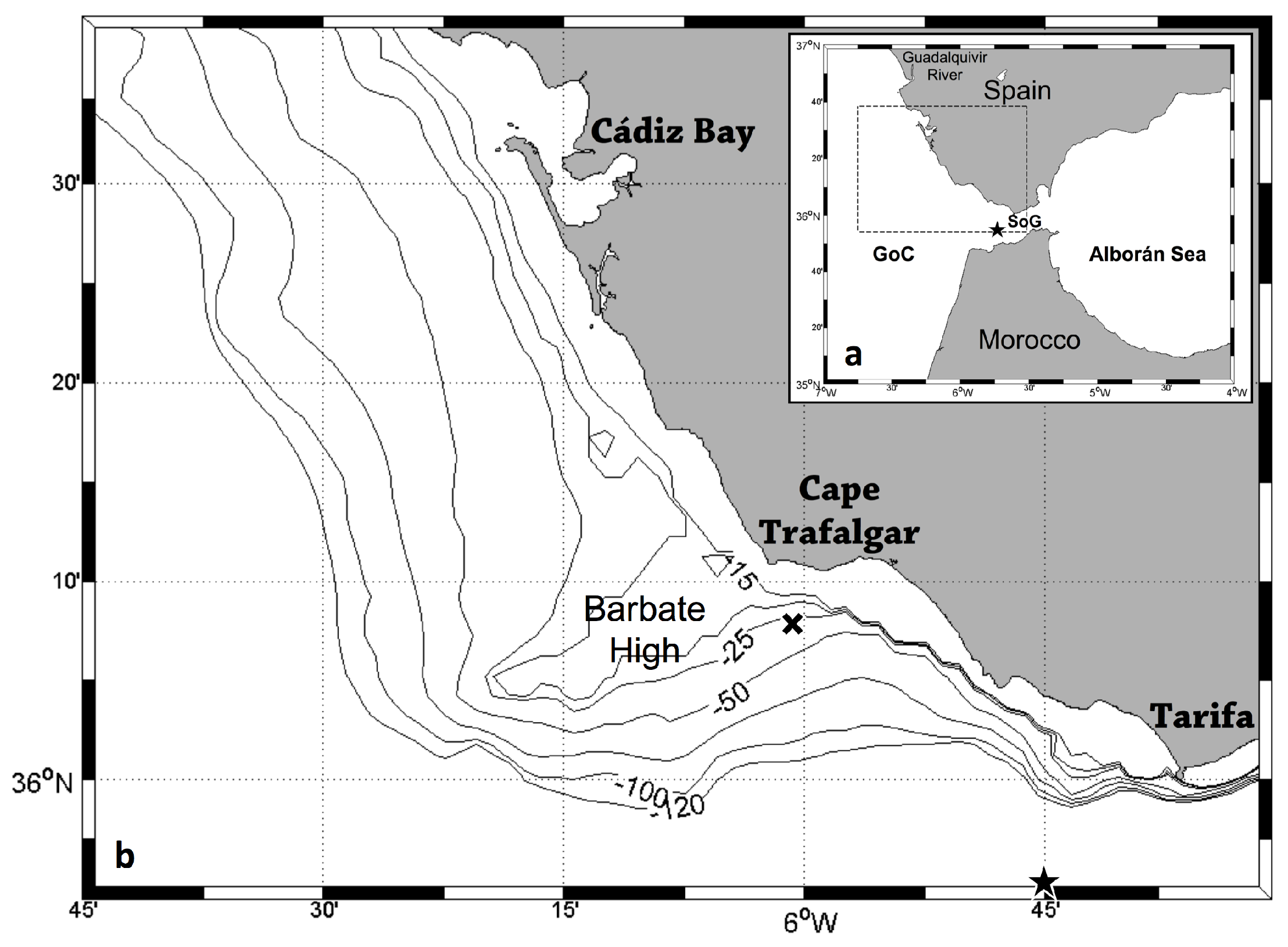
Cape Trafalgar, located along the south-western coast of the Iberian Peninsula, is the imaginary boundary that separates the Gulf of Cádiz (GoC) and the Strait of Gibraltar (SoG; Figure 1). Intricate hydrodynamics characterise these regions, with the SoG being considered one of the most oceanographically complex spots in the world (see e.g., [1,2,3,4]). The surface circulation in the GoC is influenced by one of the branches of the Azores Current that flows eastward producing a front characterised by high mesoscale variability [5,6,7], whereas the circulation through the SoG is induced by a negative hydrological budget in the Mediterranean Sea. As evaporation exceeds the sum of precipitation and river discharge [8], there is a two-layer inverse estuarine circulation that results in an upper Atlantic layer flowing towards the Alborán Sea and an outflow of deep high-density Mediterranean waters towards the Atlantic Ocean [9]. However, this general scheme increases its complexity due to a variety of phenomena such as intense and frequent wind (e.g., [10,11]), transport fluctuations due to the tidal cycles (e.g., [4,12]), or the generation of high-amplitude internal waves associated with periods of spring and neap tides (e.g., [13,14]). Furthermore, the topography strongly modifies this intricate scheme, and is particularly noticeable at the tidal scale (e.g., [15]).
Both seasonal and tidal scales of variability had already been marked as very relevant for chlorophyll distribution in the area, with an emphasis on seasonality in the GoC (see e.g., [16,17]) and mainly tidal cycles in the SoG (see e.g., [18,19]). Cape Trafalgar, located in the middle of these two regions, has been highlighted as a region with high autotrophic productivity and biomass rather associated to the nutrient input due to upwelled waters (see e.g., [20,21,22]). Here, the topography is particularly relevant. The flat and shallow platform (<50 m in depth), with an average width of ∼35 km that characterises the GoC region, decreases in width up to ∼15 km south of Cape Trafalgar. Moreover, on the northern side of the Cape there is a submarine ridge extending offshore perpendicular to the coast [23], which is an area known as the Barbate High or the “bajo de la aceitera” (meaning “boiling oil bank”; Figure 1b). Vargas-Yáñez et al. [24] studied the influence of the tide–topography interaction in the nutrient flux in this region, using in situ observations supported by a physical–biological model. Their observations showed non-symmetrical hydrological conditions on both sides of the Cape due to the abrupt change in the bathymetry towards the SoG. Furthermore, their bi-dimensional model evidenced the vertical transport of deep waters to surface layers when tidal current flowed over this topographic obstacle, even when tidal intensity was reduced. These authors concluded that the tidal–topographical interaction is the main process responsible for the pool of cool and fertilised waters around Cape Trafalgar, although several mechanisms, such as wind-driven upwelling, could enhance this effect.
However, though the singularity and relevance of Cape Trafalgar in the general distribution of chlorophyll has been already highlighted (see e.g., [16]), no study has focused on the chlorophyll dynamics of this singular region. Considering its location in the confluence zone of one region dominated by long-term seasonal variability (i.e., GoC), and another by short-term tidal variability (i.e., SoG), the aim of this work is to study the spatial and temporal variability of chlorophyll in Cape Trafalgar region at both scales. To achieve this goal, we used a 10-year dataset of surface chlorophyll-a concentration derived from the MEdium Resolution Imaging Spectrometer (MERIS). Additionally, the coupling between chlorophyll concentration variability and three different environmental variables (wind, Guadalquivir river discharge, and tidal current) was analysed in order to examine the co-variation between them.
2. Data and Methodology
2.1. Satellite Images
The satellite ocean colour images data used in this study were obtained from MERIS, an ocean colour sensor developed by the European Space Agency (ESA) that flew on board the Envisat multispectral platform. All available images of daily chlorophyll-a concentration (chl-a, mg m), at full spatial resolution (FR, 300 m) and considering the complete mission of this sensor (from September 2002 to April 2012), were downloaded via ftp (file transfer protocol) from the Ocean Color Website (http://oceancolor.gsfc.nasa.gov). The obtained Level-2 products were processed using the standard NASA methodologies, being the result of the sensor calibration and atmospheric correction of the corresponding Level-1A product. These images were read and remapped to a Mercator projection using SeaDAS (v6.4) image analysis software (http://seadas.gsfc.nasa.gov). To discard all suspicious and low-quality pixels, standard SeaDAS flags (L2_flags, [25]; Table 1) were used, ensuring that only the most reliable data was retained for analysis. Chl-a concentration was derived from the OC4Me ocean colour algorithm [26]. The MERIS-OC4Me algorithm yielded reasonable chl-a retrievals in the GoC (r = 0.96; n = 27; p < 0.0001; bias of 0.31 mg m and Root-Mean-Square Error of 0.41 mg m; [25]), although with a systematical overestimation [25] also found in this region using Moderate-Resolution Imaging Spectroradiometer (MODIS) products [27]. Finally, as extremely high chlorophyll values are not usually detected in the area of interest, only pixels with chl-a < 10 mg m were considered [16,28].
The MERIS sensor provided a global coverage every 3 days, and considering a region of interest (ROI) centred in Cape Trafalgar (between 35.90–36.64N, and 6.75–5.52W; Figure 1b), in total 5006 daily images were downloaded. However, this area is characterised by frequent cloudy conditions resulting in patchy spatial coverage and temporal gaps, and consequently 3098 of these 5006 daily images had a cloud coverage >80%. This problem was avoided when composite images were computed by simply averaging pixel-by-pixel the chl-a concentration of the corresponding daily images. Thus, a monthly climatology dataset was computed to study the spatial and temporal variability at a seasonal scale in the chl-a distribution in the Trafalgar region. Additionally, to study the influence of fortnightly tidal cycles, and with respect to the temporal evolution of spring/neap tides, 7-day composite images were produced averaging ±3 days from spring and neap tides. Considering as valid the image composites with cloud coverage <20% of sea pixels, in total 109 composite images were generated for the monthly data set, and 349 composite images for the tidal cycle dataset.
2.2. Environmental Variables
Zonal component of wind. Due to the topography of the ROI that extends mainly in an east–west direction, only the zonal component of wind (u-wind) was considered. Data was downloaded from ERA-Interim, a global atmospheric reanalysis from 1979 [29] provided by the European Center for Medium-range Weather Forecast (ECMWF; https://www.ecmwf.int/). U-wind data has a time resolution of 6 hours and a spatial resolution of 0.125 degree. However, in this study only the same data point for the mooring was considered (see below).
Guadalquivir river discharge. Daily averages (m s) from the Alcalá del Río dam, located 110 km upstream from the river mouth, were obtained from the regional water management agency (Agencia Andaluza del Agua, Junta de Andalucía, http://www.juntadeandalucia.es/agenciadelagua/saih/).
Zonal component of tidal current. In terms of wind velocity, only the zonal component of tidal current (u-tide) was considered in our analysis. Barotropic tidal current prediction was acquired from harmonic constituents and constants determined by a classical harmonic analysis [30]. The analysis was applied to current velocity measurements obtained from a Nortek Acoustic Wave and Current sensor (AWAC). The mooring was bottom-mounted (36.13N–6.03W; black cross in Figure 1b) and it was programmed to sample current profiles every 30 s with 0.5 m bin size during 45 days.
2.3. Empirical Orthogonal Function (EOF) Analysis
EOF analysis, introduced in Earth sciences by Obukhov [31] and Lorenz [32], is a useful way of organising large sets of information. The aim of the method is to simplify a spatial-temporal dataset by compressing the variability in time series data and providing a compact description of their spatial-temporal variability in terms of orthogonal functions, called empirical modes [33]. In practice, only the first few modes can account for most of the variation in a dataset.
In this work, the EOF analysis was carried out with the tidal cycle dataset, using the singular value decomposition method [34]. Since this method requires a dataset without gaps, sea pixels covered by clouds on valid image composites (i.e., with cloud coverage <20%) were replaced by the average of the surrounding pixels (3 × 3 box). In the case there were still pixels covered by clouds, the temporal mean chl-a concentration was assigned to the remaining cloud pixels. Pixels belonging to Cádiz Bay were erased in order to avoid its influence in this analysis. Finally, before the EOF analysis was performed, the temporal mean was subtracted to each pixel in order to enhance the variation of temporal patterns.
To identify the significant modes, the error distance was calculated following North et al. [35]:
where is the eigenvalue and n is the number of images used in the EOF analysis.
2.4. Wavelet Analysis
Wavelet analysis is a powerful tool that is especially relevant to the analysis of non-stationary systems (see Cazelles et al. [36] for a review). This methodology has been successfully applied in ecological time series during the past decade, achieving a local time-scale decomposition of the signal in both time and frequency domains [36,37,38,39]. Furthermore, wavelet analysis allows the estimation of the coupling between drivers and response variables as well as the level of synchrony among them [40,41,42]. This analysis was performed using the Matlab toolbox developed by Cazelles and Chavez [36] (http://www.biologie.ens.fr/~cazelles/bernard/Welcome.html). The Morlet wavelet was used in this study, which provides a good balance between time and frequency localisation [43]. In a time-frequency plane, the wavelet power spectrum (WPS) represents the relative importance of frequencies for each time step. Meanwhile, the wavelet coherence (WCo) analyses the co-variation patterns for the drivers and the response signal in time [36]. Values closer to the edge of the time series, delimited by the cone of influence, are rejected in order to avoid false periodic events. Below this cone of influence the information should be interpreted with caution [38]. For each period, the average wavelet power spectrum (WPS analysis) and the average wavelet cross-spectrum (WCo analysis) are calculated, identifying the averaged variance contained in all wavelet coefficients of the same frequency. Moreover, a 5% significance level was determined for WPS through a bootstrapping scheme using a hidden Markov model, to assess whether the wavelet-based quantities were not only due to random processes [44].
This statistical analysis was carried out with the tidal cycle dataset after computing the mean time series at three identified zones characterised by a singular dynamics (see Section 3.1). Components with periods greater than 3 years were obviated, as they could not be well resolved. In addition, WCo was applied to analyse the synchrony of the environmental variables (i.e., wind, Guadalquivir river discharge, and tidal current) with chl-a concentration in the two identified coastal zones in order to determine if there is a correlation between the different drivers (i.e., environmental variables) and the response signal (i.e., chl-a concentration). Once identified the time scale at which the two non-stationary time series were locally linearly correlated, their phases, for this time scale, were extracted and compared [36]. The phase difference between signals indicates whether or not both signals are in synchrony, and if they are not, the lag time between them.
Data preparation. The zonal component of wind and the Guadalquivir river discharge are environmental variables mainly characterised by seasonal variability. Therefore, the temporal scale to study the co-variation between both drivers and the response signal should be from seasonal to inter-annual cycles. As the chl-a tidal cycle dataset has weekly resolution, u-wind, with a 6-h resolution, and river discharge, with daily resolution, were weekly averaged prior to the application of wavelet analysis. Moreover, considering the delay of phytoplankton response to the nutrient input conducted by these drivers, the weekly average was calculated considering the 7 days prior from the spring/neap tide (several tests were performed to select the best time lag; data not shown). Finally, due to the different units and scales of measurement of all time series, they were standardised to mean zero and unit variance.
However, a weekly temporal resolution to study the co-variation of the fortnightly tidal cycle and chl-a concentration is very low. Therefore, for this analysis daily means for the two identified coastal zones (Zone 1 and Zone 2; see Section 3.1) were calculated from the original data. As mentioned before, the study area is characterised by high cloud coverage, and considering the small areas of Zone 1 and Zone 2, for this analysis, valid images were considered as those with a cloud coverage <30% (instead of <20%) of sea pixels. Three valid periods were identified for each zone, with each period lasting at least 20 days and with gaps of less than 5 days between measurements. Those gaps were filled by linear interpolation. Finally, driver and response signals were standardised to mean zero and unit variance.
3. Results
3.1. Spatial Variability
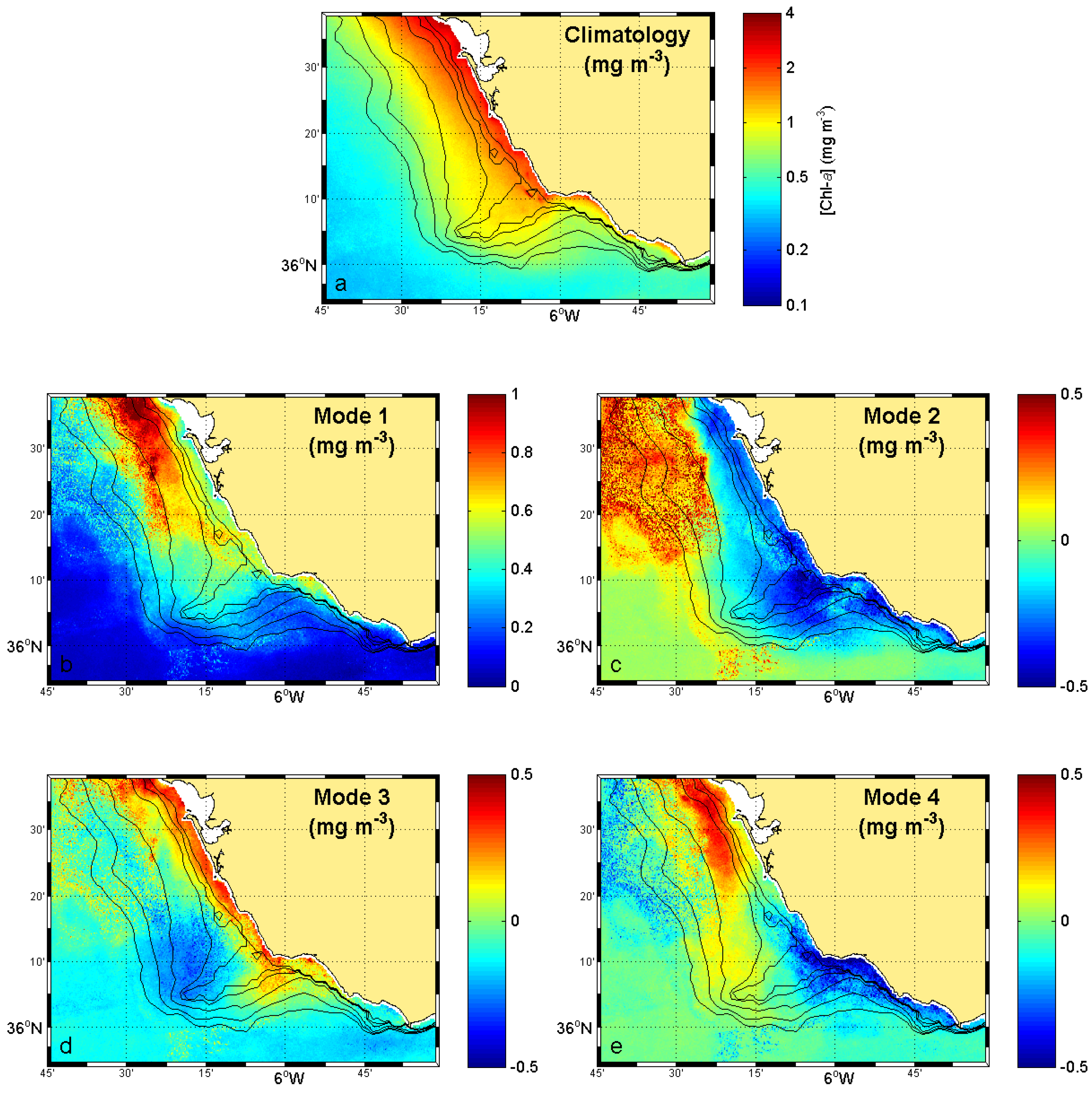
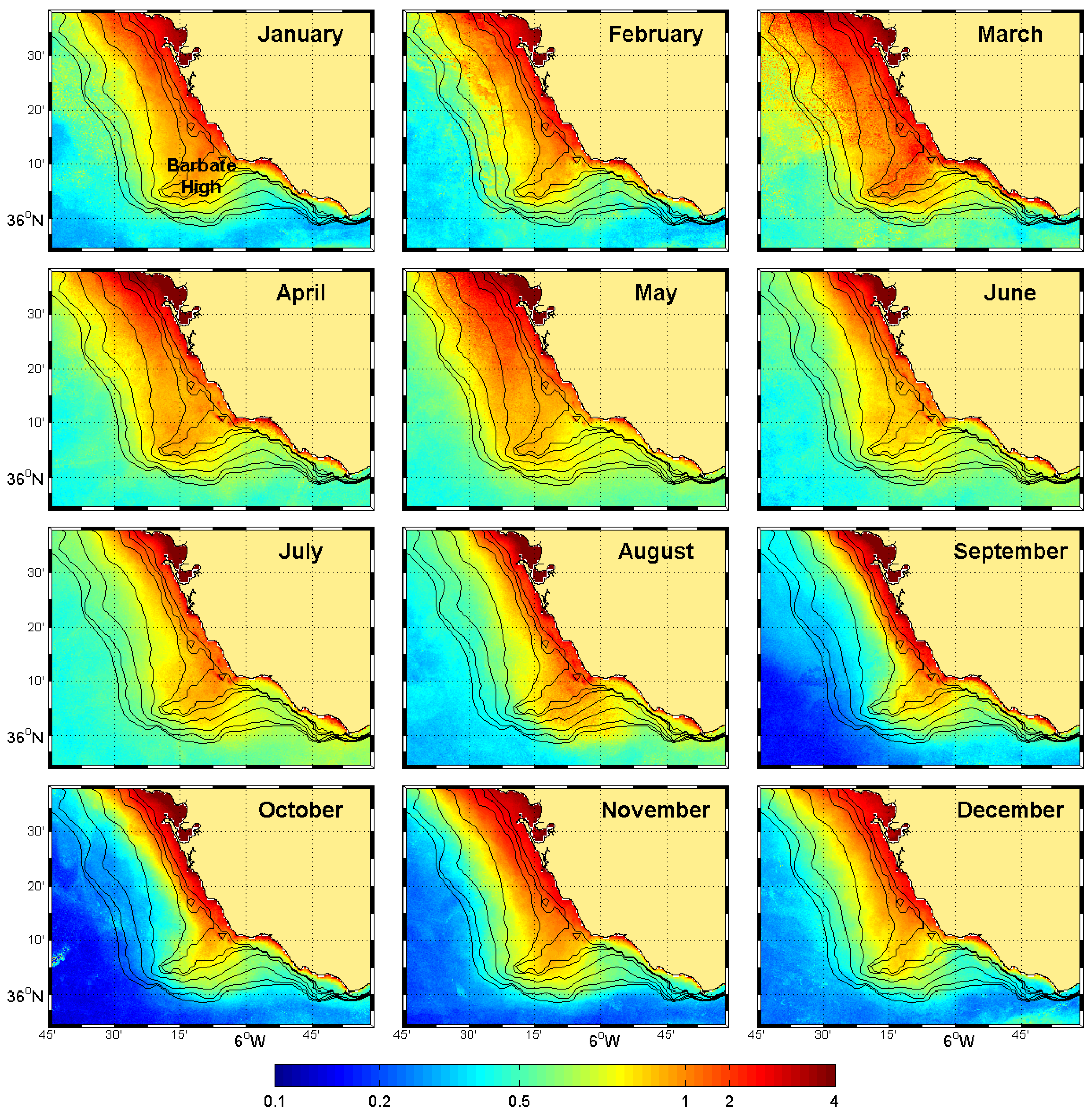
Figure 2 shows the monthly climatological distribution of the surface chl-a concentration during the whole period (10 years) in the ROI. During this period, the chl-a concentration was higher in the GoC region, north of Cape Trafalgar, than in the SoG, where it was always limited to shallow waters (<15 m depth). In the GoC region, higher chl-a concentrations were found closer to the coast, especially around Cádiz Bay. Along the whole year, there was a fringe of eutrophic waters (with chl-a>1 mg m; [45]) more or less extended over the continental shelf, lined up following the bathymetric lines. From January to May, chl-a was distributed covering the whole continental shelf with high concentrations varying between 1 and 4 mg m. While offshore, chl-a concentration was <0.5 mg m. March evidenced the highest chl-a concentration, with the dispersion of the eutrophic fringe reaching offshore waters (colours from yellow to red). From June to October, chl-a distribution across the continental shelf decreased, with the eutrophic fringe limited to ∼50 m in depth in June, until ∼25 m in October. From November to December, chl-a distribution gradually increased again spreading over the continental shelf, with this eutrophic fringe extended to ∼75–100 m. Offshore, the lowest chl-a concentrations were also found in October, with values <0.2 mg m. These low values increased gradually until December. From September to December, when the gradient of surface chl-a concentration from the coast to the open ocean was more pronounced, it was easier to appreciate the strong coupling of chlorophyll values with coastal bathymetry.
Notwithstanding, although chl-a distribution over the GoC region showed a seasonal variability throughout the climatological year (Figure 2), Cape Trafalgar was always characterised by an accumulation of chlorophyll over Barbate High. This tongue of high chl-a concentration could be more (e.g., during spring) or less developed (e.g., during fall) throughout the climatological year, but it was always present and with a chl-a concentration >1 mg m. In fact, monthly averages along the 10-year period always showed the presence of this tongue (data not shown). This region was studied later with more detail (see Section 3.2).
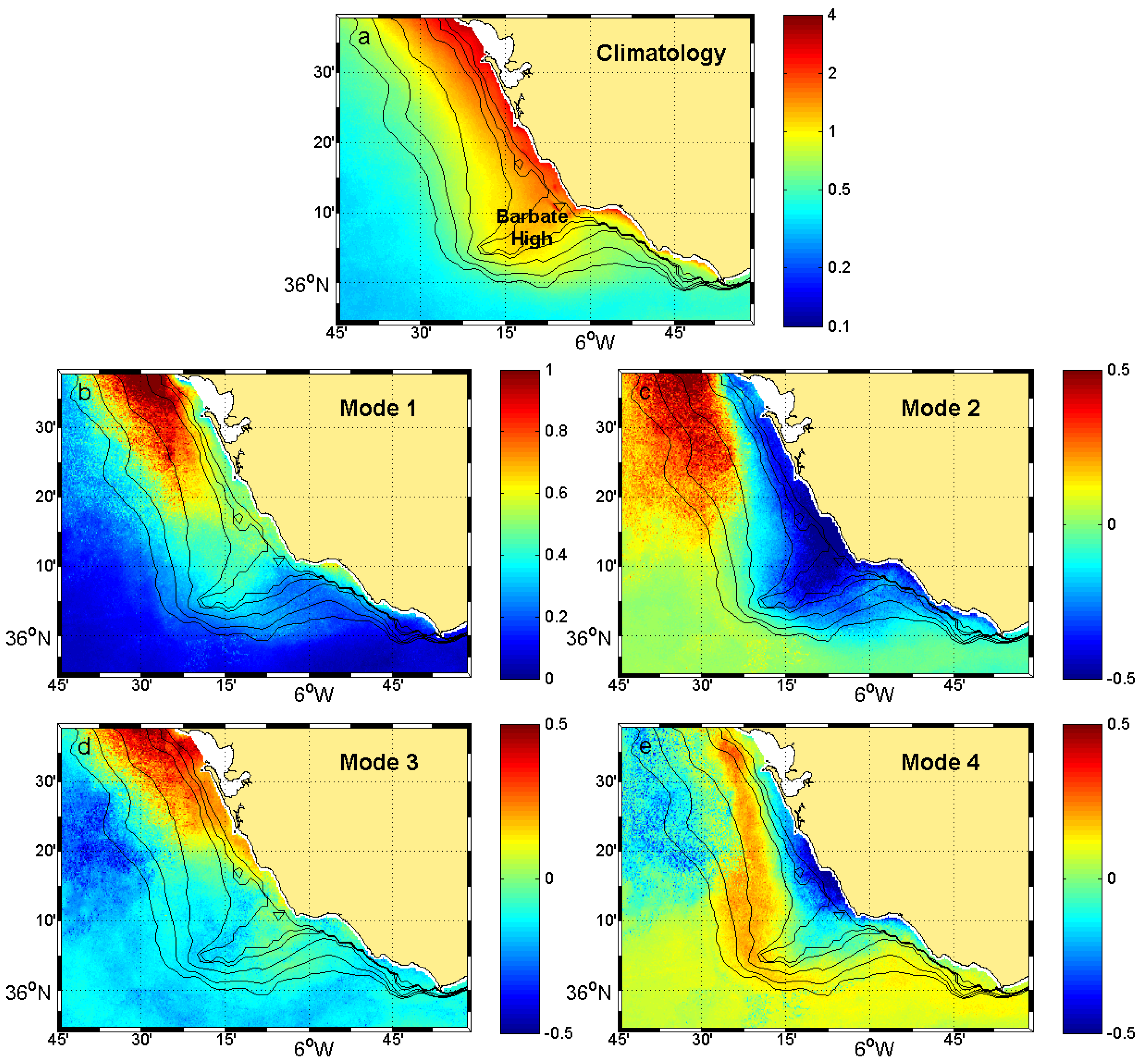
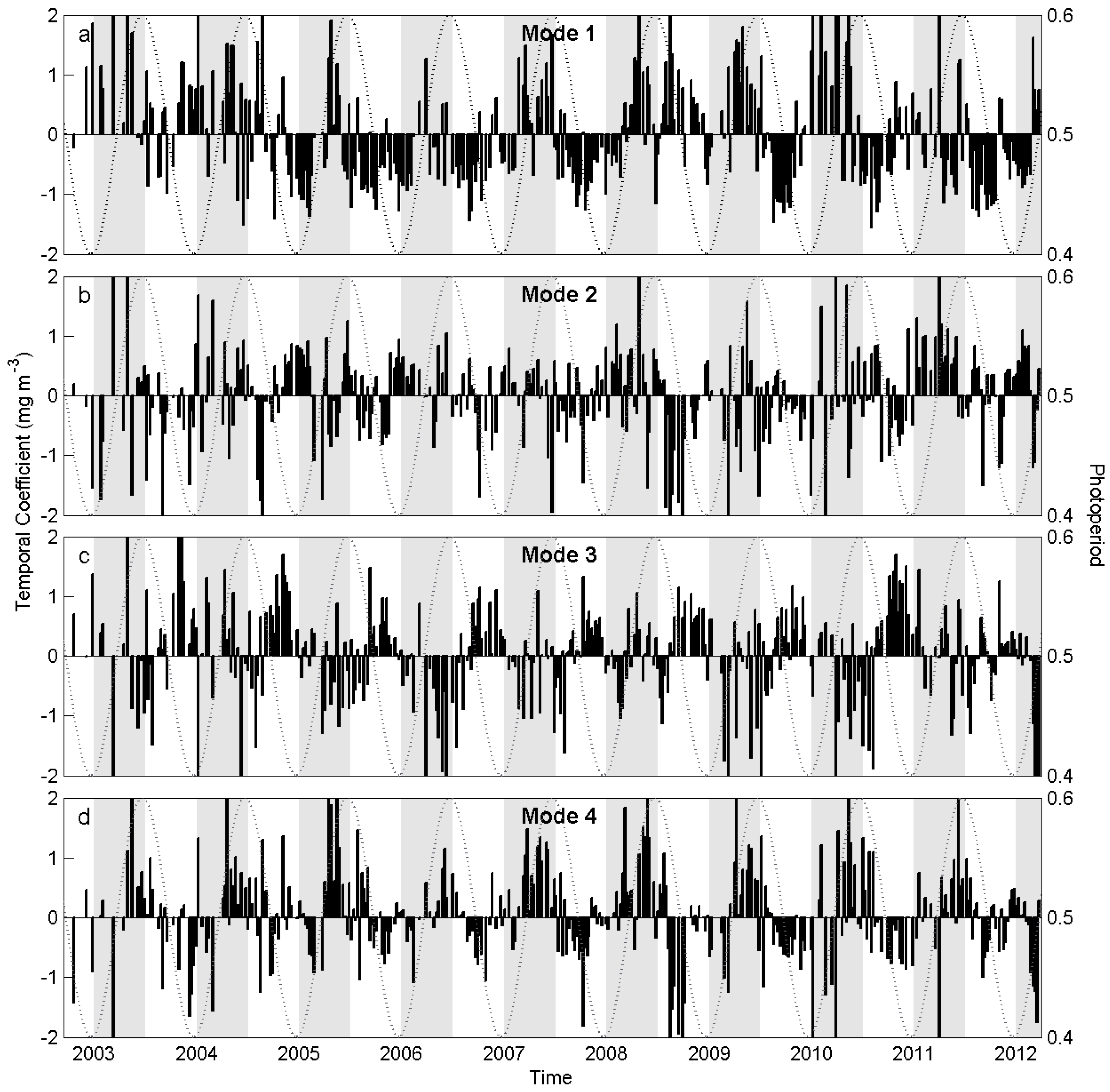
In order to study the influence of the fortnightly tidal cycle in the chl-a distribution, and considering the large amount of data available, an EOF analysis was performed because of its high capacity to organise large sets of information. The first four modes of this analysis were found to be statistically significant, representing around 58.25% of the total variance of the series. Figure 3 shows the spatial coefficient maps corresponding to these four modes, while Figure 4 shows their temporal evolution. To understand the intensity of each mode, both spatial and temporal coefficients must be taken into account. Dotted lines in Figure 4 are a representation of seasons through oscillations trends of photoperiod in order to make it easier to identify changes potentially linked to seasonality. The photoperiod was calculated following Kremer and Nixon [46]:
where day refers to the day of the year. The fraction of hours of light versus the hours of darkness per day calculated in this study is an approximation of the reality, used only as a visual guide.
The first mode explained 35.45% of the variance. All the spatial coefficients were positive, with a maximum in an area in front of Cádiz Bay (Figure 3b). These positive spatial values, while with a lower coefficient, reached Barbate High, delimitating a northern oceanographic region within the ROI. A spatial coefficient of 0, indicates a high stability of surface chl-a with respect to the rest of the ROI. The accumulation of chl-a in this region increased when temporal amplitudes were positive, and decreased when negative. The temporal coefficient for this mode is directly correlated with chl-a concentration in the red zone (R = 0.84; data not shown). Although it is difficult to appreciate even with the photoperiod information, along the whole period, positive values appear to be more frequently associated to winter and spring, and negative values to summer and fall (Figure 4a). This seasonal variability mainly associated with chl-a variability in the red zone, was later confirmed with the wavelet analysis (see Section 3.2).
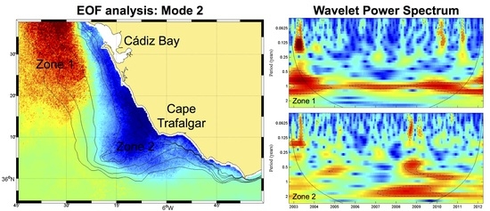
Mode 2 explained 11.59% of the variance. This mode identified two areas with a dynamical response of different phase (Figure 3c). The first one, with positive values, was located in front of Cádiz Bay and it was overlapped with the red zone identified in the first mode. Here, chl-a concentration increased when temporal amplitudes were positive, and decreased when negative. The second one, a zone with negative values, was located in front of Cape Trafalgar lined up with bathymetry. Here, the chl-a concentration increased when temporal amplitudes were negative, and decreased when positive. Outside both areas, the spatial coefficient was 0, implying a small variability. Temporal amplitudes did not show a clear pattern of variability (Figure 4b).
Mode 3 explained 7.27% of the variance. The distribution of the spatial coefficients was very similar to Mode 1 (Figure 3d). However, in this mode the red zone in front of Cádiz Bay was closer to the coast. A second zone, with negative values, was located also in front of Cádiz Bay, but offshore. Temporal amplitudes (Figure 4c) followed a seasonal pattern, with negative values in winter becoming positive at fall, where the values were maximum.
Only 3.94% of the variance was explained by Mode 4. This mode highlighted an area of high chl-a concentration close to the coast between Cádiz Bay and Cape Trafalgar (Figure 3e). This area, although smaller, coincided with the blue area of Mode 2. Another zone with negative values dispersed and less intense was located occupying the same blue zone found in Mode 3, offshore in front of Cádiz Bay. A third zone in opposition phase was located between the other two. Temporal amplitude also showed a seasonal pattern, with positive values in spring and negative in fall (Figure 4d).
3.2. Temporal Variability
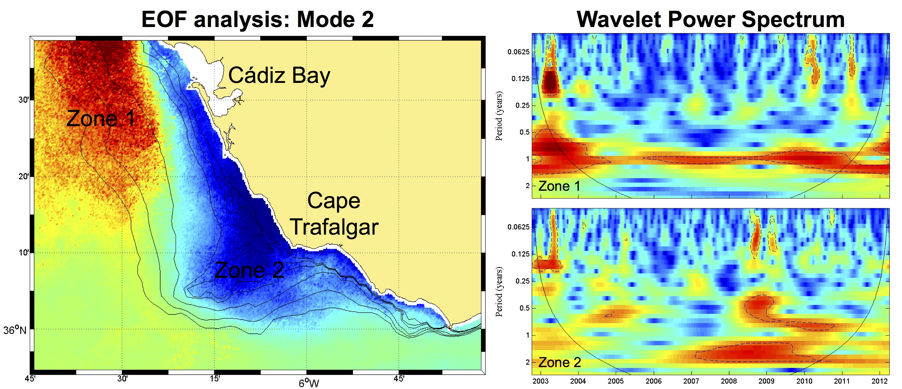
Considering our especial interest in studying the singularity of Cape Trafalgar, based on Mode 2 from EOF analysis, three different study zones were identified: Zone 1, Zone 2, and the Open Ocean (Figure 5). For each zone, a weekly chl-a time series was computed from the tidal cycle dataset to examine and extract information about their temporal variability. The characterisation of these non-stationary series was performed by a wavelet power spectrum analysis.
Open Ocean. Figure 6a shows chl-a time series computed for this area. For the whole period, the mean chl-a concentration was 0.76 mg m (dotted line), typical for mesotrophic waters (0.1–1.0 mg m; [45]). However, only in ∼21% of the cases was the chl-a concentration over this value (Figure 6b), with a minimum of 0.15, and a maximum of 2.45 mg m. The WPS of this time series evidenced a strong 1-year periodic component (Figure 6c). This signal was statistically significant in the whole period, and represented on average ∼30% of the total variance (Figure 6d). A second peak, with a low average power spectrum, was found at the temporal cycle between 3 and 6 months (0.125–0.25 year). For this temporal cycle, high power values could be found at the beginning of 2003 and 2004 (Figure 6c), coinciding with high concentration peaks in the area (Figure 6a).
Zone 1. Located in front of Cádiz Bay (Figure 5), Zone 1 was highlighted in the first three EOF modes, although varying its position more or less close to coast. In Zone 1, chl-a concentration varied along the 10-year period, with an average value of 0.79 mg m, typical for mesotrophic waters, reaching a minimum of 0.10 and a maximum value of 6.34 mg m (Figure 7a). This average value was surpassed only in ∼35% of the cases (Figure 7b). In this zone, the WPS also showed a clear 1-year periodic component (Figure 7c), although it was less powerful than in Open Ocean, representing on average ∼23% of the total variance (Figure 7d). This annual component was discontinuous along the 10-year period. In 2005 the power of this signal was weaker and not statistically significant. There was also a weak signal in the 3–6 month (0.125–0.25 year) temporal cycle. The highest power value was found at the beginning of 2003, when chl-a concentrations in Zone 1 reached maximum values.
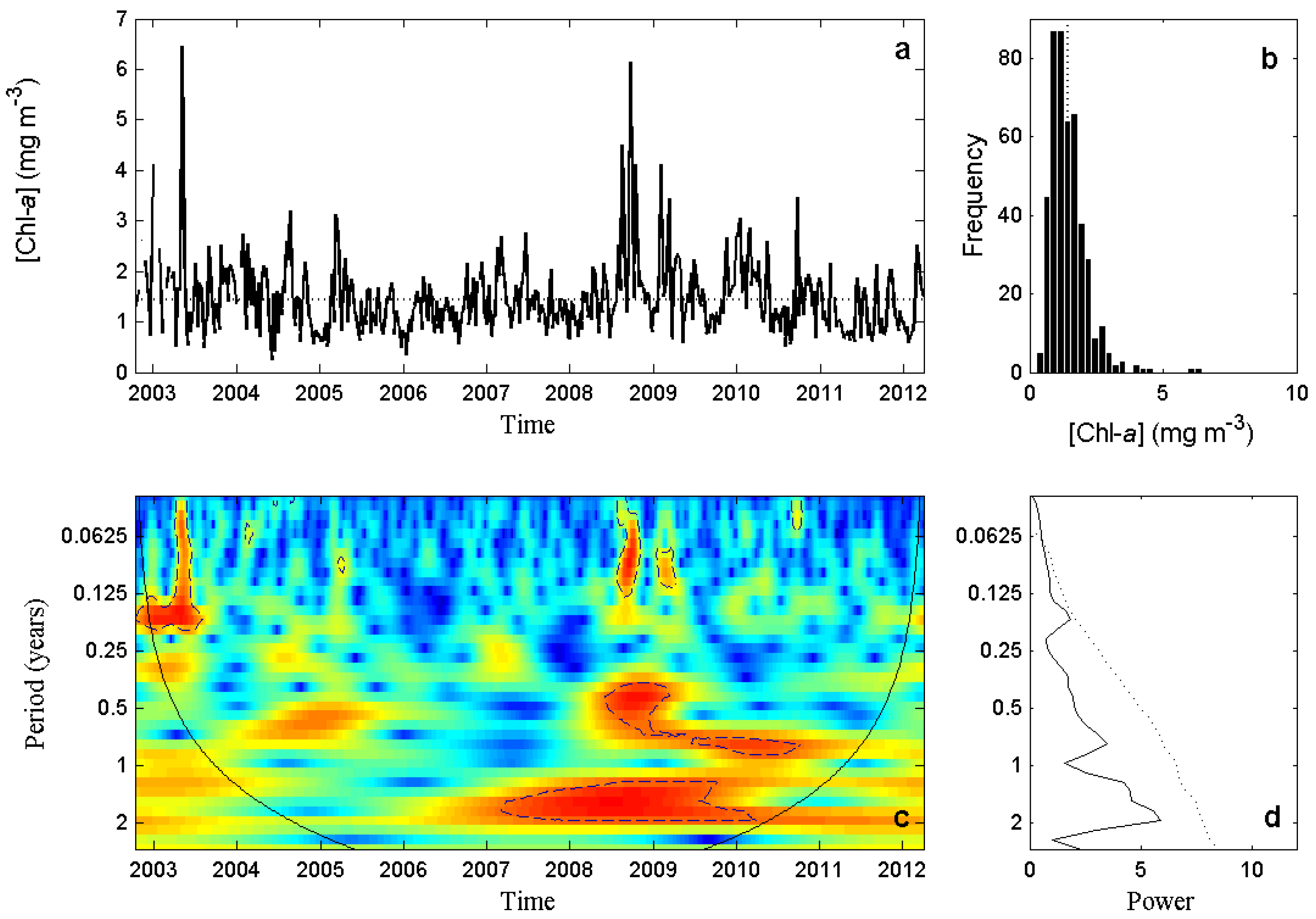
Zone 2. This zone characterises the dynamics in Cape Trafalgar (Figure 5), located close to shallow coast. Zone 2 stood out mainly in the second EOF mode, although in the third one it was also partially present. The average chl-a concentration along the whole period was 1.44 mg m, a value within the range for eutrophic waters (1.00–10.0 mg m; [45]), with a minimum value of 0.25 and a maximum of 6.45 mg m (Figure 8a). In ∼45% of the cases, this average value was surpassed (Figure 8b). For this zone, the WPS displayed peaks of high power signal at different periods (Figure 8c). Notwithstanding, the 1-year periodic component showed a low power value (Figure 8d). The highest power was found in the band between the 1.5 and 2-year component, with a strong and statistically significant signal between ∼2007 and 2010. However, this maximum had an averaged power value half of the peaks observed for the other zones. Another peak of the power spectrum appeared in the band of ∼10-months, with a strong signal between ∼2009 and 2011 (Figure 8c). As in the wavelet analysis for Open Ocean and Zone 1, a peak was found at the beginning of 2003 in the 3–6 month (0.125–0.25 year) temporal cycle, coinciding again with a high chl-a concentration in Zone 2. At the end of 2008 and beginning of 2009, there were two signals with high power coinciding with high chl-a concentration, although more centred in the 1.5–3 month (0.0625–0.125 year) temporal cycle.
3.3. Chlorophyll Concentration Dynamics and Environmental Variables
To better understand the role of some environmental variables in the dynamics of chl-a in both coastal zones (Zone 1 and Zone 2), a wavelet coherence analysis was performed. With this methodology, the co-variation patterns (the degree of linear relationship) for u-wind, Guadalquivir river discharge, and u-tide versus chl-a concentration, were analysed. The consistency of the coherence between the different drivers and chl-a concentration was identified from the average wavelet cross-spectrum. Once the most consistent period for each pair of signals (i.e., the highest cross-spectrum power value) was identified, the corresponding oscillations were extracted for the whole period to compare their amplitudes and phases.
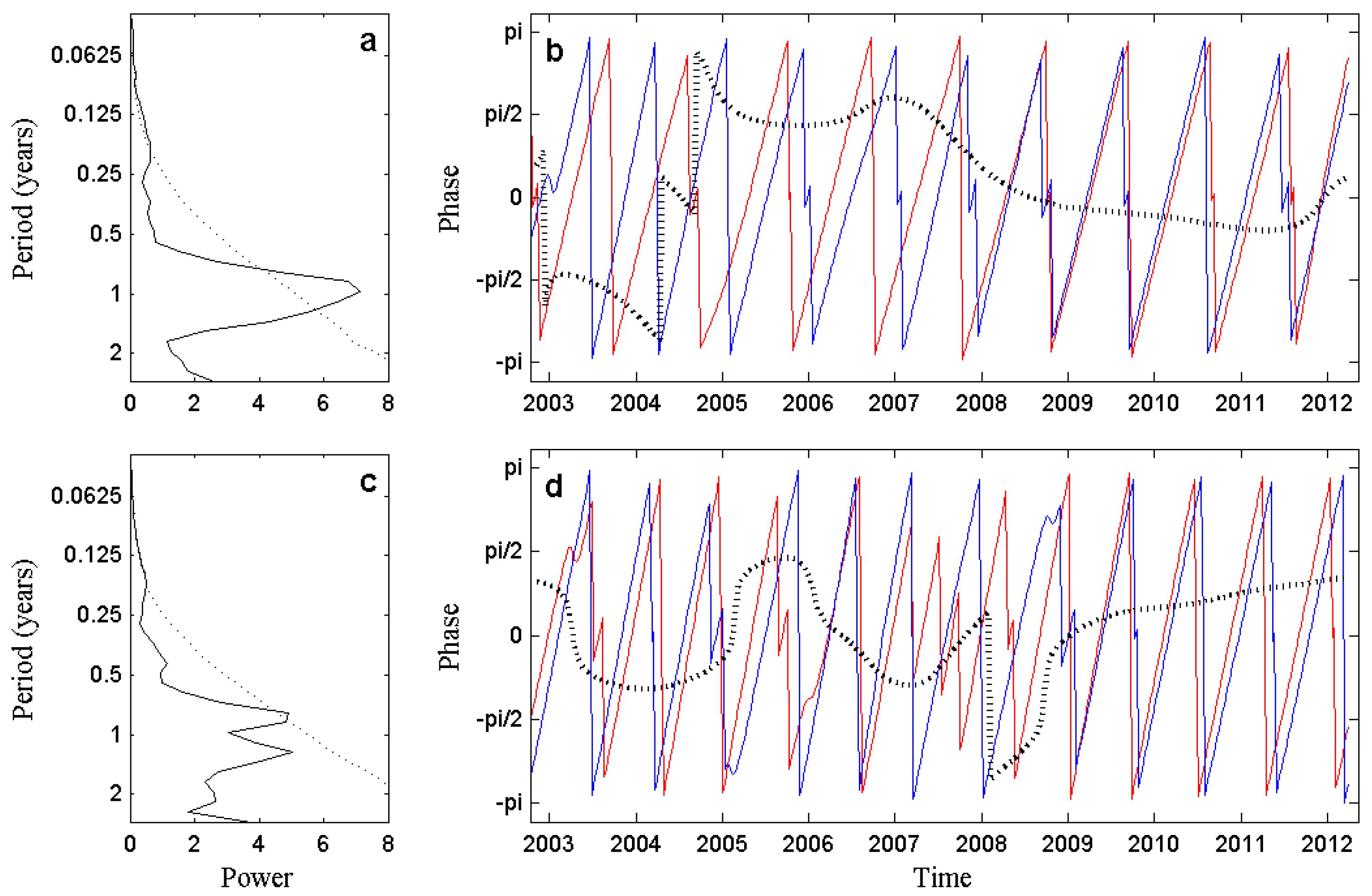
Zonal component of wind. Weekly time series for both u-wind and chl-a concentration variables were used to perform this WCo analysis (see Section 2.4). The strongest coherence between chl-a in Zone 1 and u-wind was found at the annual scale (Figure 9a), with a cross-spectrum power value of ∼3.45 (Table 2). As not all the area under this peak was statistically significant, this information should be interpreted with caution. Between 2003 and 2004, and from ∼2009 onwards, there was a 3-month (i.e., /2) delay between signals. From 2004 to 2009, the sign of the association between chl-a and u-wind changed with a maximum delay of ∼1.5-months, with the chl-a signal appearing before the driver’s signal, revealing a weak coherence at the annual scale (Figure 9b). The coherence between chl-a concentration in Zone 2 and u-wind showed different peaks of similar cross-spectrum power along the analysed period, in ∼10 and ∼15-month periods (Figure 9c). In this case, phase differences were evaluated for the ∼10-month cycle, with a slightly higher cross-spectrum power value of ∼2.34 (Table 2). At the beginning of the study period there was a small delay between signals that disappeared, showing synchrony among them from ∼2004 to 2007. Between 2007 and 2009 there was a delay between the coinciding signals, with a period of high chl-a concentration in this zone. Thereafter, both signals recovered their synchrony (Figure 9d).
Guadalquivir river discharge. WCo analysis of the relationship between Guadalquivir river discharge and chl-a concentration was also performed using weekly time series (see Section 2.4). Guadalquivir river discharge and chl-a concentration in Zone 1 showed the strongest coherence at an annual scale (Figure 10a), with a cross-spectrum power value of ∼6.94 (Table 2). Again, this information should be interpreted with caution, as not all the area under the peak was statistically significant. From ∼2004 to 2008, the phase differences had a ∼3-month delay (i.e., /2; Figure 10b), with a positive sign, appearing the chl-a signal before than the driver’s signal. From 2008, both signals were almost in synchrony (Figure 10b). The average wavelet cross-spectrum between river discharge and Zone 2 showed again two peaks with high values, at ∼10 and ∼15 months (Figure 10c). The oscillation between signals was extracted at a ∼10-month scale (Figure 10d), with a cross-spectrum power value of ∼4.88 (Table 2). From the beginning of the period to 2009, the phase difference among signals oscillated between positive and negative values. In 2009 both signals were synchronised, but from 2010 onwards they lost this synchrony progressively.
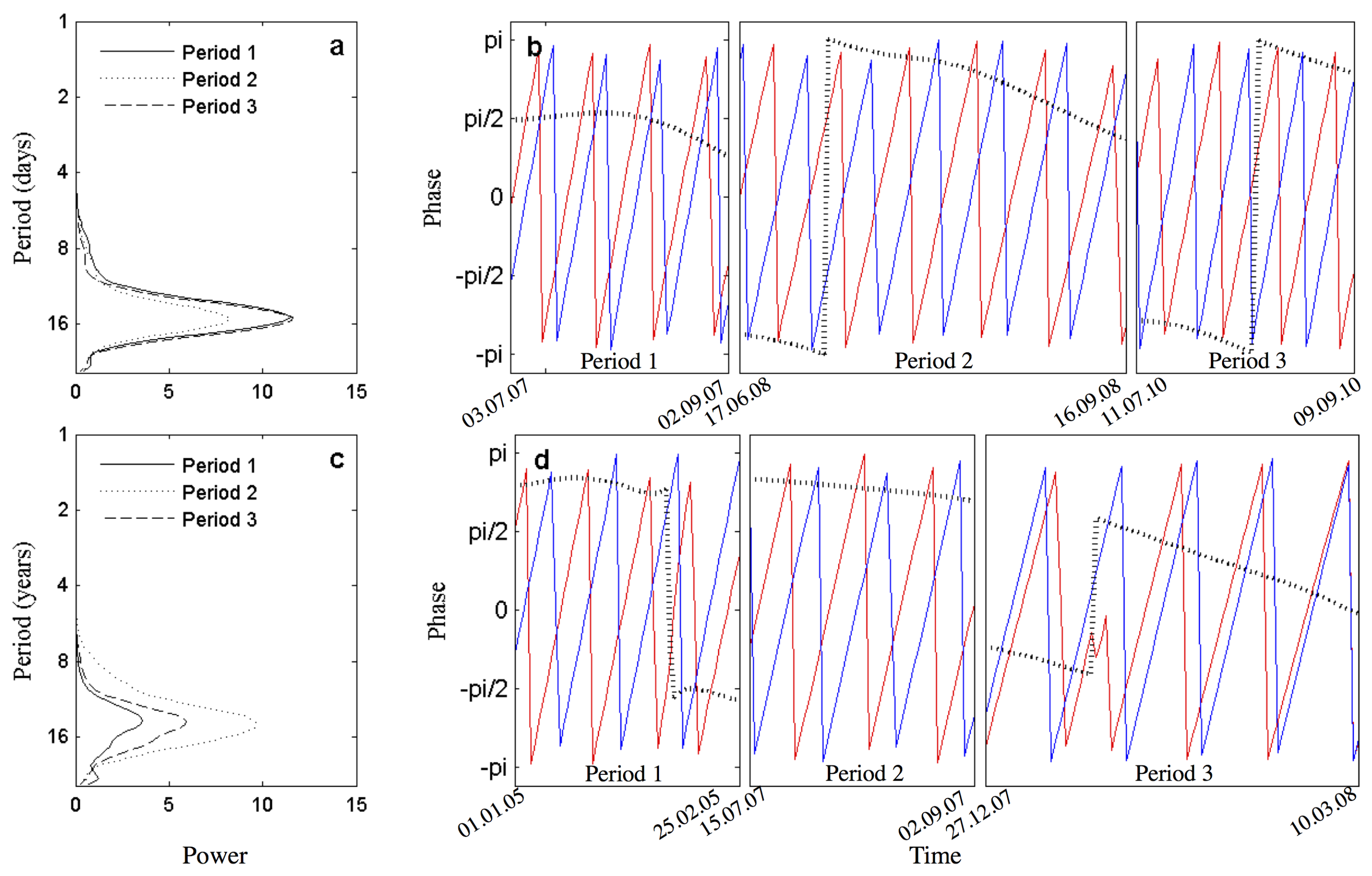
Zonal component of tidal current. To study the co-variation patterns between the u-tide and chl-a concentration, three valid periods for each zone, with daily resolution, were analysed (see Section 2.4). For Zone 1, the three identified periods were from 3 July to 2 September 2007 (Period 1); from 17 June to 16 September 2008 (Period 2); and from 11 July to 9 September 2010 (Period 3). For the three periods, the co-variation between u-tide and chl-a concentration in Zone 1 was particularly consistent at the 15-day scale, with a cross-spectrum power value very similar between them (Figure 11a). Mean power value for the three periods (∼10.31; Table 2) explained ∼45% of the total variance. However, in none of the periods were the driver and response synchronised (Figure 11b). The delay between them was ∼7-days (i.e., ), being the response signal before in time than the driver. At the beginning of Period 2 and Period 3, u-tide’s signal appeared prior to that of chl-a with a delay of 7 days. For Zone 2, the three identified periods were from 2 July to 2 September 2007 (Period 1); from 27 December 2007 to 10 March 2008 (Period 2); and from 14 June to 14 September 2008 (Period 3). In this case, the 15-day scale was the most consistent (Figure 11c). For Zone 2, the mean power values were lower than for Zone 1 (∼5.99; Table 2), explaining ∼36% of the variance. For the three periods, drivers and responses were out of phase, with a delay ∼7-days (Figure 11d). Except for the beginning of Period 3, and the end of Period 1 and Period 3, the response signal appeared before in time than the driver.
4. Discussion
Several studies have highlighted Cape Trafalgar as a spot of high chlorophyll concentration, from in situ data collected in several surveys (e.g., [47]) as well as remote sensing studies (e.g., [16]). The peculiarity of this hotspot lies not only in the fact that it is framed between two regions distinguished by different dynamics—the GoC mainly characterised by long-term seasonal variability, and the SoG highly influenced by the tidal cycle—but also because of its bathymetry [24]. The interaction of the tidal cycle with bathymetry allows the upwelling of cold and nutrient-rich waters [24,48,49,50,51]. Phytoplankton, characterised by fast-growing cells, responds rapidly to this tidal-induced mixing that fertilises illuminated surface waters. Moreover, Cape Trafalgar, due to the dominant mesoscale circulation has been identified as an area with high water residence time [52], acting as a biomass core [47]. However, the focused interest in this hotspot is not only due to the complex hydrodynamics and physical–biological interactions based on its unique geographic framework. Cape Trafalgar is assumed to act as a source of biomass exporting chlorophyll and nutrient rich waters towards the Alborán Sea. Sub-mesoscale processes have been identified as important mechanisms in the chlorophyll distribution between coastal zones and the main channel of the SoG [19,52], along with the transport of nutrients to the Mediterranean Sea [14], highlighting mainly the role of the fortnightly tidal cycle [12,47]. A lateral advection of coastal waters into the centre of the channel takes place when internal waves are generated over the Camarinal Sill (Figure 1a) during the spring tides [12,52], and also, although it is less evident, during the release of arrested internal waves during neap tides [47]. These pulsating events play an important role in the nutrient and biomass input of the Alborán Sea [53,54,55], which has a natural tendency to oligotrophy due to its negative hydrological budget [9,56,57].
Seasonal variability found in Zone 1, initially revealed by the climatological maps (Figure 2), was confirmed by EOF analysis (Figure 3 and Figure 4), as well as wavelet analysis (Figure 7). This variability could be explained by the upwelling of cold and nutrient-rich waters characteristic of the south-western Iberian shelf [11,22,58,59], the seasonal wind-induced variability [11], and the available light intensity. The extension of the upwelling varies throughout seasons, increasing until early winter (e.g., December–January) when the upwelling area reaches Cape Trafalgar. Moreover, high Guadalquivir river discharge is expected during the fall and winter. Thus, westerlies, more common during these seasons, tend to extend the upwelling influence to the east and favour the transport of Guadalquivir river discharge towards Cádiz Bay. Meanwhile, during the spring and summer, the upwelling extension decreases gradually until April, being confined west and out of our ROI until August [11]. Easterlies, especially during spring and summer, induce an upwelling in our ROI, west of the SoG [11]. Our results showed how the extension of chl-a over the continental shelf increased gradually from September to February, coinciding with the evolution of the upwelling. Although from January the upwelling extension starts to decrease, the combination of wind and the increment of available light intensity would allow the increase in concentration and extension of chl-a during spring months. Meanwhile, during the summer when light intensity is not limiting, chl-a distribution decreased gradually, probably due to the fact that influence of easterlies is restricted to shallower waters.
The Open Ocean and Zone 1 showed very similar results in the wavelet analysis, although the annual signal for the coastal zone was weaker (Figure 6 and Figure 7). Drivers like tides, wind, or river discharge, have more impact on coastal areas than offshore (e.g., tidal mixing can enlarge the productive season; [60]), introducing variability to the system and weakening the seasonal signal. This fact coincides with the presence of Zone 1 in several modes of the EOF analysis, highlighting the complexity of this coastal zone (Figure 3 and Figure 4). WCo analysis performed between both seasonal drivers (u-wind, and Guadalquivir river discharge) and chl-a concentration in Zone 1 showed an intense co-variation at an annual scale (Figure 9a and Figure 10a), the co-variation being stronger with river discharge (Table 2). Meanwhile, u-wind and chl-a signals in Zone 1 were never synchronised (Figure 9b). The co-variation with Guadalquivir river discharge showed a period of minimum delay (∼1-month) between 2009 and 2012 (Figure 10b) coinciding with extremely high river discharge [61,62]. After these periods of high river discharge there is a coupling between sediment resuspension and phytoplankton blooms, with satellite data overestimating chl-a in situ concentrations [25]. This scenario would be aggravated during extremely high river discharge, so these results should be interpreted with caution. However, Krug et al. [63], using Ocean Colour Climate Change Initiative Group (OC-CCI; http://www.esa-oceancolour-cci.org) chl-a product (Case I waters) and applying generalised additive mixed models, also identified the direct influence of Guadalquivir river discharge in the chl-a concentration variability in this zone, as well as the less intense influence of wind.
Zone 2, or Barbate High, located in front of Cape Trafalgar, was characterised by the presence of a tongue of high chlorophyll concentration present along the whole climatological year (Figure 2). This zone was slightly influenced by Mode 1 of the EOF analysis (Figure 3b), with a weak seasonal variability probably overshadowed by other stronger signals. However, this zone, really highlighted in Mode 2, perfectly lined up with bathymetry (Figure 3c). Preliminary EOF analysis performed with a dataset that only included chl-a concentration during spring tides and another one that only included chl-a concentration during neap tides, showed Mode 2 with a stronger Zone 2 for the spring tides dataset (Figure A1), and a weaker and slightly more dispersed Zone 2 for the neap tides dataset (Figure A2). For this reason, this mode may be related with the influence of the fortnightly tidal cycle. However, the temporal coefficients for Mode 2, or even the wavelet analysis, did not show a clear pattern of variability (Figure 4b and Figure 8c,d). In fact, WPS analysis evidenced how irregular the chl-a dynamics were in Zone 2. Notwithstanding, the WCo analysis between the u-tide and chl-a concentration in Zone 2 showed a strong linear relationship at the fortnightly scale (Figure 11c). Although the tidal–bathymetry interaction is greater in Zone 2 than in Zone 1, a stronger cross-spectrum value was obtained for Zone 1. Longer valid periods were found for Zone 1, perhaps affecting the obtained results. However, for Zone 1, the longest valid period (Period 2) showed the lowest cross-spectrum value (Figure 11a); meanwhile, for Zone 2, the longest period (Period 3) showed an intermediate value (Figure 11c). Hence, this difference between the zones could be related with the intricate hydrodynamics that characterise the Cape Trafalgar region. Anyhow, the driver and response showed a ∼7-day delay in both areas, this being a necessary lag time for phytoplankton to respond to the new input of nutrients.
Chl-a concentration variability in Zone 2 was also correlated with the seasonal drivers. Co-variation with both drivers (u-wind and Guadalquivir river discharge), was stronger at the ∼10-month scale (Figure 9a and Figure 10a), again with a higher linear correlation with river discharge (Table 2). U-wind and chl-a in Zone 2 showed a quite synchronised co-variation (Figure 9b,d). The influence of easterlies in our ROI was greater than the influence of westerlies [11,64]. East winds enhance the upwelling of nutrient-rich waters, being more noticeable in Zone 2 together with tidal–bathymetry interaction. Co-variation between Guadalquivir river discharge and chl-a in Zone 2, as in Zone 1, showed a period of minimum delay between 2009 and 2012 (Figure 10d) coinciding with extremely high river discharge. The general circulation in the GoC [65,66] and the influence of westerlies [11] would convey the Guadalquivir river discharge along the continental shelf towards Cape Trafalgar. However, only during the period characterised by very high Guadalquivir river discharge were both signals close to synchrony.
The co-variation between both seasonal drivers and chl-a in Zone 2 showed two peaks with very similar cross-spectrum power values, meanwhile the u-tide showed a single and strong peak. Furthermore, the total variance explained by the ∼10-month peak of seasonal drivers was lower (∼11%) than the total variance explained by the 15-day peak of the u-tide (∼36%; Table 2). These differences between seasonal drivers and u-tide reveal a stronger correlation between u-tide and chl-a concentration variability in Zone 2.
5. Conclusions
In this study, satellite data spanning 10 years was analysed in order to understand the singular dynamics of Cape Trafalgar. The results revealed two coastal areas which displayed completely different dynamics, although they are mainly coastal and very close one to another. Both areas were influenced by seasonal variability, wind-induced variability, tidal-induced variability, and river discharge. Notwithstanding, bathymetry was the main feature differentiating the physical–biological interaction occurring in Zone 1 and Zone 2.
Zone 1, located in front of Cádiz Bay in a flat and shallow shelf with an average width of ∼35 km, showed a clear seasonal variability in the distribution and concentration of surface chl-a along the GoC coast. Although Zone 1 did not lose its seasonality along the whole period, this signal was weakened by the influence of the other environmental variables.
Meanwhile, Zone 2 was characterised by the presence of a submarine ridge extending offshore perpendicular to the coast, a feature that interacts with parallel coastal currents driven by tides [24]. Although Zone 2 was characterised by a quasi-permanent high chl-a concentration, it did not show a clear pattern of variability. The u-tide showed the strongest correlation with chl-a variability in this zone. The tidal–bathymetry interaction would lead to strong local mixing, increasing the availability of nutrients and, consequently sustaining phytoplankton blooms in this region [24,48,67]. In addition, this input of nutrient-rich waters could be enhanced by other environmental variables introducing noise into the chl-a concentration variability, thus masking any possible pattern of variability.
This study identifies Cape Trafalgar (Zone 2) as crucial for sustained primary production in the region, and reveals how the intricate hydrodynamics of the area affect the spatial and temporal variability of chl-a concentration as well as the evolution of this proxy of productivity with the selected drivers. However, to better understand its complexity, the effect of these drivers should be quantified. The physical–biological interactions described in this area produce a deep chl-a peak that is not detectable by satellites [48,68,69]. Moreover, these deep chlorophyll maxima in the SoG have been related with the interfaces of different water masses [28,70]. Therefore, to further understand the influence of these drivers in Trafalgar region, the analysis of field samples and modelling exercises would be desirable.
Acknowledgments
The authors thank Lucie Buttay for her support with the wavelet analysis. They also acknowledge the ESA and NASA for providing access to MERIS images. The Spanish National Research Plan through projects, CTM2013-49048, CTM2014-58181-R, and Regional Project PR11-RNM-7722 have supported this work. Iria Sala and Marina Bolado-Penagos are supported by a grant of the FPI fellowship program. Comments provided by four anonymous reviewers substantially improved subsequent versions of the manuscript.
Author Contributions
G.N., I.S., C.M.G., and F.E. designed the study. I.S. and G.N. analysed and interpreted the data. M.B.-P. processed the barotropic tidal prediction. I.S. wrote the manuscript. All authors discussed the results and contributed to the manuscript.
Conflicts of Interest
The authors declare no conflict of interest.
Appendix A
Figure A1.
Spatial coefficient maps corresponding to the first four modes of the empirical orthogonal function (EOF) analysis performed with the spring tides dataset.
Figure A1.
Spatial coefficient maps corresponding to the first four modes of the empirical orthogonal function (EOF) analysis performed with the spring tides dataset.
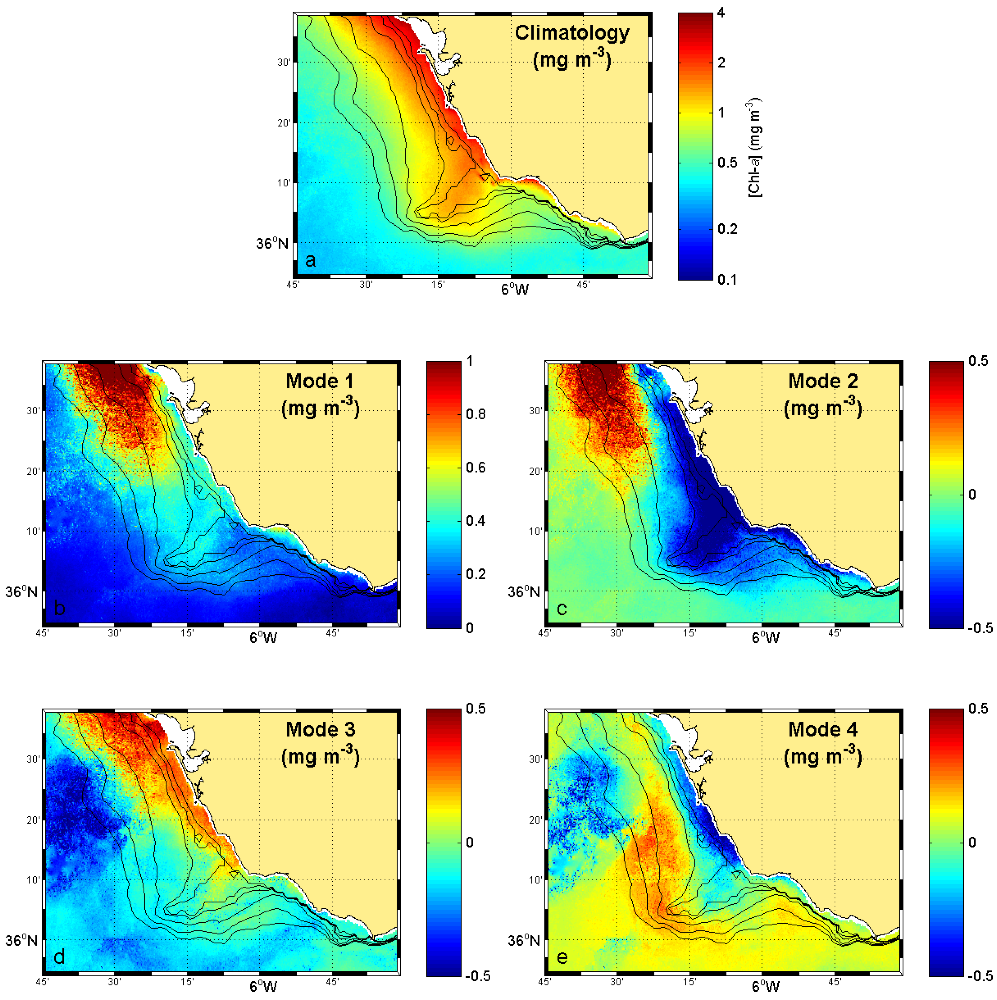
Figure A2.
Spatial coefficient maps corresponding to the first four modes of the EOF analysis performed with the neap tides dataset.
Figure A2.
Spatial coefficient maps corresponding to the first four modes of the EOF analysis performed with the neap tides dataset.
References
- Viúdez, A.; Haney, R.L. On the relative vorticity of the Atlantic jet in the Alborán Sea. J. Phys. Oceanogr. 1997, 27, 175–185. [Google Scholar] [CrossRef]
- La Violette, P.E.; Lacombe, H. Tidal-induced pulses in the flow through the Strait of Gibraltar. Oceanol. Acta 1988, 13–27. Available online: http://www.dtic.mil/dtic/tr/fulltext/u2/a207824.pdf (accessed on 7 December 2017).
- García-Lafuente, J.; Vargas, J.M.; Plaza, F.; Sarhan, T.; Candela, J.; Bascheck, B. Tide at the eastern section of the Strait of Gibraltar. J. Geophys. Res. 2000, 105, 14197–14213. [Google Scholar] [CrossRef] [Green Version]
- Bruno, M.; Alonso, J.J.; Cózar, A.; Vidal, J.; Ruiz-Cañavate, A.; Echevarría, F.; Ruiz, J. The boiling-water phenomena at Camarinal Sill, the Strait of Gibraltar. Deep Sea Res. Part II 2002, 49, 4097–4113. [Google Scholar] [CrossRef]
- Fernández, E.; Pingree, R.D. Coupling between physical and biological fields in the North Atlantic subtropical front southeast of the Azores. Deep Sea Res. Part I 1996, 43, 1369–1393. [Google Scholar] [CrossRef]
- Martins, C.S.; Hamann, M.; Fiúza, A.F. Surface circulation in the eastern North Atlantic, from drifters and altimetry. J. Geophys. Res. 2002, 107, 1–22. [Google Scholar] [CrossRef]
- Sala, I.; Caldeira, R.M.; Estrada-Allis, S.N.; Froufe, E.; Couvelard, X. Lagrangian transport pathways in the northeast Atlantic and their environmental impact. Limnol. Oceanogr. 2013, 3, 40–60. [Google Scholar] [CrossRef]
- Béthoux, J. Budgets of the Mediterranean Sea: Their dependence on the local climate and on the characteristics of the Atlantic waters. Oceanol. Acta 1979, 2, 157–163. [Google Scholar]
- Armi, L.; Farmer, D.M. The flow of Mediterranean water through the Strait of Gibraltar. Prog. Oceanogr. 1988, 21, 1–105. [Google Scholar]
- García-Lafuente, J.; Delgado, J.; Vargas, J.M.; Varela, M.; Plaza, F.; Sarhan, T. Low frequency variability of the exchanged flows through the Strait of Gibraltar during CANIGO. Deep Sea Res. Part II 2002, 49, 4051–4067. [Google Scholar] [CrossRef]
- Vargas, J.M.; García-Lafuente, J.; Delgado, F.C. Seasonal and wind-induced variability of Sea Surface Temperature patterns in the Gulf of Cádiz. J. Mar. Syst. 2003, 38, 205–219. [Google Scholar] [CrossRef]
- Macías, D.; García, C.M.; Echevarría, F.; Vázquez, A.; Bruno, M. Tidal induced variability of mixing processes on Camarinal Sill (Strait of Gibraltar): A pulsating event. J. Mar. Syst. 2006, 60, 177–192. [Google Scholar] [CrossRef]
- Vázquez, A.; Bruno, M.; Izquierdo, A.; Macías, D.; Ruiz-Cañavate, A. Meteorologically forced subinertial flows and internalwave generation at the main sill of the Strait of Gibraltar. Deep Sea Res. Part I 2008, 55, 1277–1283. [Google Scholar] [CrossRef]
- Bruno, M.; Chioua, J.; Romero, J.; Vázquez, A.; Macías, D.; Dastis, C.; Ramírez-Romero, E.; Echevarría, F.; Reyes, J.; García, C.M. The importance of submesoscale processes for the exchange of properties through the Strait of Gibraltar. Progr. Oceanogr. 2013, 116, 66–79. [Google Scholar] [CrossRef]
- García-Lafuente, J.; Sánchez-Román, A.; Díaz del Rí, G.; Sannino, G.; Sánchez-Garrido, J.C. Recent observations of seasonal variability of the Mediterranean outflow in the Strait of Gibraltar. J. Geophys. Res. 2007, 112, 1–11. [Google Scholar]
- Navarro, G.; Ruiz, J. Spatial and temporal variability of phytoplankton in the Gulf of Cádiz through remote sensing images. Deep Sea Res. Part II 2006, 53, 1241–1260. [Google Scholar] [CrossRef]
- García-Lafuente, J.; Ruiz, J. The Gulf of Cádiz pelagic ecosystem: A review. Progr. Oceanogr. 2007, 74, 228–251. [Google Scholar] [CrossRef]
- Bruno, M.; Macías, J.; González-Vida, J.M.; Vázquez, A. Analyzing the tidal-related origin of subinertial flows through the Strait of Gibraltar. J. Geophys. Res. 2010, 115, 1–13. [Google Scholar] [CrossRef]
- Macías, D.; Navarro, G.; Echevarría, F.; García, C.M.; Cueto, J. Phytoplankton pigment distribution in the northwestern Alborán Sea and meteorological forcing: A remote sensing study. J. Mar. Res. 2007, 65, 523–543. [Google Scholar] [CrossRef]
- Prieto, L.; García, C.M.; Corzo, A.; Segura, J.R.; Echevarría, F. Phytoplankton, bacterioplankton and nitrate reductase activity distribution in relation to physical structure in the northern Alborán Sea and Gulf of Cádiz (southern Iberian Peninsula). Boletin Instituto Espanol de Oceanografia 1999, 15, 401–411. [Google Scholar]
- Echevarría, F.; García-Lafuente, J.; Bruno, M.; Gorsky, G.; Goutx, M.; González, N.; García, C.M.; Gómez, F.; Vargas, J.M.; Picheral, M.; et al. Physical-biological coupling in the Strait of Gibraltar. Deep Sea Res. Part II 2002, 49, 4115–4130. [Google Scholar] [CrossRef]
- García, C.M.; Prieto, L.; Vargas, M.; Echevarría, F.; García-Lafuente, J.; Ruiz, J.; Rubín, J.P. Hydrodynamics and the spatial distribution of plankton and TEP in the Gulf of Cádiz (SW Iberian Peninsula). J. Plankton Res. 2002, 24, 817–833. [Google Scholar] [CrossRef]
- Lobo, F.; Hernández-Molina, F.; Somoza, L.; Rodero, J.; Maldonado, A.; Barnolas, A. Patterns of bottom current flow deduced from dune asymmetries over the Gulf of Cádiz shelf (southwest Spain). Mar. Geol. 2000, 164, 91–117. [Google Scholar] [CrossRef]
- Vargas-Yáñez, M.; Sarhan Viola, T.; Jorge, F.P.; Rubín, J.P.; García-Martínez, M.C. The influence of tide-topography interaction on low-frequency heat and nutrient fluxes. Application to Cape Trafalgar. Cont. Shelf Res. 2002, 22, 115–139. [Google Scholar] [CrossRef]
- Caballero, I. Estudio de Procesos en La Desembocadura del Guadalquivir y Golfo de Cádiz: Variabilidad Espacio-Temporal Mediante Teledetección. Ph.D. Thesis, University of Granada, Granada, Spain, 2015. [Google Scholar]
- Morel, A.; Antoine, D. Pigment Index Retrieval in Case 1 waters. MERIS Algorithm Theor. Basis Doc. 2000, 4, 9–25. [Google Scholar]
- Caballero, I.; Morris, E.P.; Prieto, L.; Navarro, G. The influence of the Guadalquivir River on spatio-temporal variability of suspended solid and chlorophyll in the eastern Gulf of Cádiz. Mediterr. Mar. Sci. 2014, 15, 721–738. [Google Scholar] [CrossRef]
- Navarro, G.; Ruiz, J.; Huertas, I.E.; García, C.M.; Criado-Aldeanueva, F.; Echevarría, F. Basin-scale structures governing the position of the deep fluorescence maximum in the Gulf of Cádiz. Deep Sea Res. Part II 2006, 53, 1261–1281. [Google Scholar] [CrossRef]
- Dee, D.; Uppala, S.; Simmons, A.; Berrisford, P.; Poli, P.; Kobayashi, S.; Andrae, U.; Balmaseda, M.; Balsamo, G.; Bauer, P.; et al. The ERA-Interim reanalysis: configuration and performance of the data assimilation system. Q. J. R. Meteorol. Soc. 2011, 137, 553–597. [Google Scholar] [CrossRef]
- Pawlowicz, R.; Beardsley, B.; Lentz, S. Classical tidal harmonic analysis including error estimates in MATLAB using T_TIDE. Comput. Geosci. 2002, 28, 929–937. [Google Scholar] [CrossRef]
- Obukhov, A. Statistically homogeneous fields on a sphere. Usp. Mat. Nauk 1947, 2, 196–198. [Google Scholar]
- Lorenz, E. Empirical orthogonal functions and statistical weather prediction. In Scientific Report No. 1, Statistical Forecasting Project; Department of Meteorology: Cambridge, MA, USA, 1956; Volume 1. [Google Scholar]
- Thomson, R.E.; Emery, W.J. Data Analysis Methods in Physical Oceanography; Elsevier: Amsterdam, The Netherlands, 1998. [Google Scholar]
- Kelly, K.A. Comment on “Empirical orthogonal function analysis of advanced very high resolution radiometer surface temperature patterns in Santa Barbara Channel” by G.S.E. Lagerloef and R.L. Bernstein. J. Geophys. Res. 1988, 93, 15753–15754. [Google Scholar] [CrossRef]
- North, G.R.; Bell, T.L.; Cahalan, R.F.; Moeng, F.J. Sampling errors in the estimation of empirical orthogonal functions. Mon. Weather Rev. 1982, 110, 699–706. [Google Scholar] [CrossRef]
- Cazelles, B.; Chavez, M.; Berteaux, D.; Ménard, F.; Vik, J.O.; Jenouvrier, S.; Stenseth, N.C. Wavelet analysis of ecological time series. Oecologia 2008, 156, 287–304. [Google Scholar] [CrossRef] [PubMed]
- Lau, K.M.; Weng, H. Climate signal detection using wavelet transform: How to make a time series sing. Bull. Am. Meteorol. Soc. 1995, 76, 2391–2402. [Google Scholar] [CrossRef]
- Torrence, C.; Compo, G.P. A practical guide to wavelet analysis. Bull. Am. Meteorol. Soc. 1998, 79, 61–78. [Google Scholar] [CrossRef]
- Klvana, I.; Berteaux, D.; Cazelles, B. Porcupine feeding scars and climatic data show ecosystem effects of the solar cycle. Am. Nat. 2004, 164, 283–297. [Google Scholar] [CrossRef] [PubMed]
- Ménard, F.; Marsac, F.; Bellier, E.; Cazelles, B. Climatic oscillations and tuna catch rates in the Indian Ocean: A wavelet approach to time series analysis. Fish. Oceanogr. 2007, 16, 95–104. [Google Scholar] [CrossRef]
- Keitt, T.H.; Fischer, J. Detection of scale-specific community dynamics using wavelets. Ecology 2006, 87, 2895–2904. [Google Scholar] [CrossRef]
- Buttay, L.; Cazelles, B.; Miranda, A.; Casas, G.; Nogueira, E.; González-Quirós, R. Environmental multi-scale effects on zooplankton inter-specific synchrony. Limnol. Oceanogr. 2017, 62, 1355–1365. [Google Scholar] [CrossRef]
- Grinsted, A.; Moore, J.; Jevrejeva, S. Application of the cross wavelet transform and wavelet coherence to geophysical time series. Nonlinear Process. Geophys. Eur. Geosci. Union 2004, 11, 561–566. [Google Scholar] [CrossRef]
- Cazelles, B.; Stone, L. Detection of imperfect population synchrony in an uncertain world. J. Anim. Ecol. 2003, 72, 953–968. [Google Scholar] [CrossRef]
- Franz, B.A.; Bailey, S.W.; Meister, G.; Werdell, P.J. Consistency of the NASA Ocean Color Data Record. In Proceedings of the Ocean Optics, Glasgow, UK, 8–12 October 2012. [Google Scholar]
- Kremer, J.; Nixon, S. A Coastal Marine Ecosystem: Simulation and Analysis; Springer: Berlin/Heidelberg, Germany, 1978. [Google Scholar]
- Ramírez-Romero, E.; Macías, D.; Bruno, M.; Reyes, E.; Navarro, G.; García, C.M. Submesoscale, tidally-induced biogeochemical patterns in the Strait of Gibraltar. Estuar. Coast. Shelf Sci. 2012, 101, 24–32. [Google Scholar] [CrossRef] [Green Version]
- Pingree, R.D.; Mardell, G.; Cartwright, D. Slope turbulence, internal waves and phytoplankton growth at the Celtic Sea shelf-break. Philos. Trans. R. Soc. Lond. A 1981, 302, 663–682. [Google Scholar] [CrossRef]
- New, A.; Pingree, R.D. Large-amplitude internal soliton packets in the central Bay of Biscay. Deep Sea Res. 1990, 37, 513–524. [Google Scholar] [CrossRef]
- Tee, K.; Smith, P.; LeFraive, D. Topographic upwelling off Southwest Nova Scotia. J. Phys. Oceanogr. 1993, 23, 1703–1726. [Google Scholar] [CrossRef]
- Pereira, A.; Belém, A.; Castro, B.M.; Geremias, R. Tide-topography interaction along the eastern Brazilian shelf. Cont. Shelf Res. 2005, 25, 1521–1539. [Google Scholar] [CrossRef]
- Vázquez, A.; Flecha, S.; Bruno, M.; Macías, D.; Navarro, G. Internal waves and short-scale distribution patterns of chlorophyll in the Strait of Gibraltar and Alborán Sea. Geophys. Res. Lett. 2009, 36. [Google Scholar] [CrossRef]
- Packard, T.T.; Minas, H.; Coste, B.; Martínez, R.; Bonin, M.; Gostan, J.; Garfield, P.; Christensen, J.; Dortch, Q.; Minas, M.; et al. Formation of the Alborán oxygen minimum zone. Deep Sea Res. 1988, 35, 1111–1118. [Google Scholar] [CrossRef]
- Minas, H.; Coste, B.; Le Corre, P.; Minas, M.; Raimbault, P. Biological and geochemical signatures associated with the water circulation through the Strait of Gibraltar and in the Western Alborán Sea. J. Geophys. Res. 1991, 96, 8755–8771. [Google Scholar] [CrossRef]
- Macías, D.; Martin, A.P.; García-Lafuente, J.; García, C.M.; Yool, A.; Bruno, M.; Vázquez, A.; Izquierdo, A.; Sein, D.V.; Echevarría, F. Analysis of mixing and biogeochemical tides on the Atlantic-Mediterranean effects induced by flow in the Strait of Gibraltar through a physical-biological coupled model. Prog. Oceanogr. 2007, 74, 252–272. [Google Scholar] [CrossRef]
- Lacombe, H.; Richez, C. The regime of the Strait of Gibraltar. In Elsevier Oceanography Series; Nihoul, J.C., Ed.; Elsevier: Amsterdam, The Netherlands, 1982; Volume 34, pp. 13–73. [Google Scholar]
- Hopkins, T.S. The thermohaline forcing of the Gibraltar exchange. J. Mar. Syst. 1999, 20, 1–31. [Google Scholar] [CrossRef]
- Fiúza, A.F.; de Macedo, M.; Guerreiro, M. Climatological space and time variation of the Portuguese coastal upwelling. Oceanol. Acta 1982, 5, 31–40. [Google Scholar]
- Fiúza, A.F.G. Upwelling Patterns off Portugal. In Coastal Upwelling Its Sediment Record; Suess, E., Thiede, J., Eds.; Springer: Boston, MA, USA, 1983; Volume 10B, pp. 85–98. [Google Scholar]
- Simpson, J.H.; Hunter, J.R. Fronts in the Irish Sea. Nature 1974, 250, 404–406. [Google Scholar] [CrossRef]
- Navarro, G.; Huertas, I.E.; Costas, E.; Flecha, S.; Díez-Minguito, M.; Caballero, I.; López-Rodas, V.; Prieto, L.; Ruiz, J. Use of a real-time remote monitoring network (RTRM) to characterize the Guadalquivir estuary (Spain). Sensors 2012, 12, 1398–1421. [Google Scholar] [CrossRef] [PubMed] [Green Version]
- Ruiz, J.; Polo, M.J.; Díez-Minguito, M.; Navarro, G.; Morris, E.P.; Huertas, I.E.; Caballero, I.; Contreras, E.; Losada, M.A. The Guadalquivir estuary: A hot spot for environmental and human conflicts. In Environmental Management and Governance; Finkl, C., Makowski, C., Eds.; Coastal Research Library Springer: Cham, Switzerland, 2015; Volume 8. [Google Scholar]
- Krug, L.A.; Platt, T.; Sathyendranath, S.; Barbosa, A.B. Unravelling region-specific environmental drivers of phytoplankton across a complex marine domain (off SW Iberia). Remote Sens. Environ. 2017, 203, 162–184. [Google Scholar] [CrossRef]
- Stanichny, S.; Tigny, V.; Stanichnaya, R.; Djenidi, S. Wind driven upwelling along the African coast of the Strait of Gibraltar. Geophys. Res. Lett. 2005, 32. [Google Scholar] [CrossRef]
- Criado-Aldeanueva, F.; García-Lafuente, J.; Vargas, J.M.; del Río, J.; Vázquez, A.; Reul, A.; Sánchez, A. Distribution and circulation of water masses in the Gulf of Cádiz from in situ observations. Deep Sea Res. Part II 2006, 53, 1144–1160. [Google Scholar] [CrossRef]
- Criado-Aldeanueva, F.; García-Lafuente, J.; Navarro, G.; Ruiz, J. Seasonal and interannual variability of the surface circulation in the eastern Gulf of Cádiz (SW Iberia). J. Geophys. Res. 2009, 114. [Google Scholar] [CrossRef]
- Pingree, R.D.; Mardell, G.; New, A. Propagation of internal tides from the upper slopes of the Bay of Biscay. Nature 1986, 321, 154–158. [Google Scholar] [CrossRef]
- Holligan, P.; Pingree, R.D.; Mardell, G. Oceanic solitons, nutrient pulses and phytoplankton growth. Nature 1985, 314, 348–350. [Google Scholar] [CrossRef]
- Lezama-Ochoa, A.; Irigoien, X.; Chaigneau, A.; Quiroz, Z.; Lebourges-Dhaussy, A.; Bertrand, A. Acoustics reveals the presence of a macrozooplankton biocline in the Bay of Biscay in response to hydrological conditions and predator-prey relationships. PLoS ONE 2014, 9, e88054. [Google Scholar] [CrossRef] [PubMed] [Green Version]
- Macías, D.; Bruno, M.; Echevarría, F.; Vázquez, A.; García, C.M. Meteorologically-induced mesoscale variability of the north-western Alborán Sea (southern Spain) and related biological patterns. Estuar. Coast. Shelf Sci. 2008, 78, 250–266. [Google Scholar] [CrossRef]
Figure 1.
(a) Location map of the Gulf of Cádiz (GoC), Strait of Gibraltar (SoG), and the Alborán Sea. The dashed line frames the region of interest of this study, located in the south-west of Spain. (b) Bathymetry of Cape Trafalgar region. Black solid lines represent the bathymetry (15, 20, 25, 50, 75, 100, 120 m). The black cross represents the mooring location (36.13N–6.03W). The black star represents the location of Camarinal Sill (35.91N–5.74W).

Figure 2.
Monthly climatology of MERIS-OC4Me chlorophyll-a concentration (mg m) centred on the Cape Trafalgar region. Black lines represent the bathymetry (15, 20, 25, 50, 75, 100, 120 m).
Figure 2.
Monthly climatology of MERIS-OC4Me chlorophyll-a concentration (mg m) centred on the Cape Trafalgar region. Black lines represent the bathymetry (15, 20, 25, 50, 75, 100, 120 m).

Figure 3.
Empirical orthogonal function analysis of fortnightly tidal cycle dataset of MERIS-OC4Me chlorophyll-a concentration (mg m). (a) Fortnightly tidal cycle climatology. Spatial coefficients maps for the (b) first, (c) second, (d) third, and (e) fourth mode. Black lines represent the bathymetry (15, 20, 25, 50, 75, 100 m). Pixels belonging to Cádiz Bay were erased in order to avoid their influence in this analysis.

Figure 4.
Empirical orthogonal function analysis of fortnightly tidal cycle dataset of MERIS-OC4Me chlorophyll-a concentration (mg m). Temporal coefficient evolution for the (a) first, (b) second, (c) third, and (d) fourth mode. Dotted lines represent the photoperiod, calculated as the fraction of hours of light versus the hours of darkness per day (Equation (2)). Grey background represents winter and spring seasons versus white background, representing summer and autumn seasons.

Figure 5.
Location of the study zones distinguished by the empirical orthogonal function analyses: Zone 1 (coastal zone in front of Cádiz Bay), Zone 2 (Cape Trafalgar region), and the Open Ocean. Pixels belonging to Cádiz Bay were erased in order to avoid its influence in this analysis.
Figure 5.
Location of the study zones distinguished by the empirical orthogonal function analyses: Zone 1 (coastal zone in front of Cádiz Bay), Zone 2 (Cape Trafalgar region), and the Open Ocean. Pixels belonging to Cádiz Bay were erased in order to avoid its influence in this analysis.
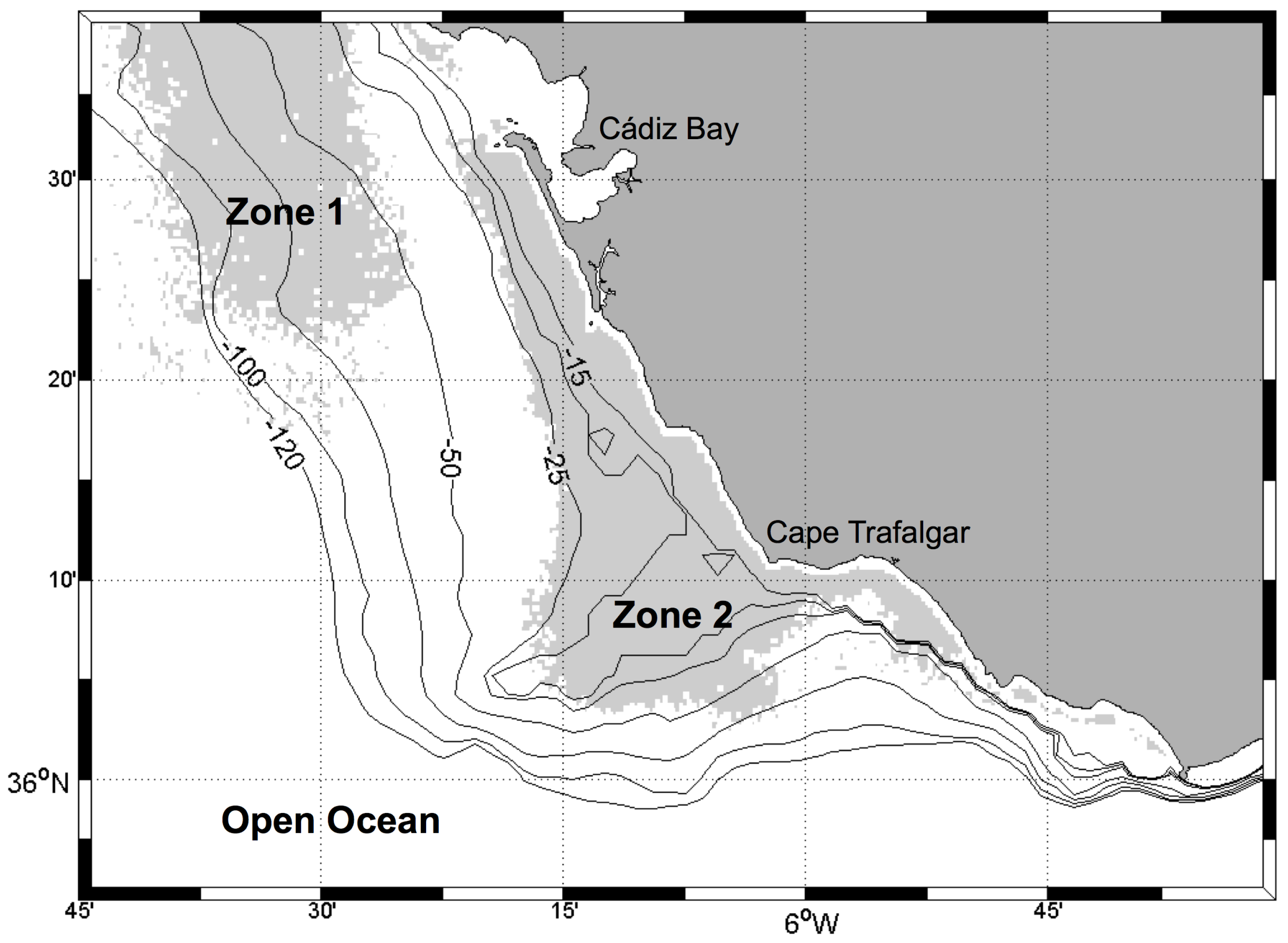
Figure 6.
Analysis of the chlorophyll-a concentration (chl-a; mg m) time series computed for the Open Ocean. (a) Temporal series of tidal cycle dataset chl-a concentration. (b) Distribution of chl-a concentration. Dotted lines (a,b) show average chl-a concentration. (c) Wavelet power spectrum. The colour code varies from dark blue (low values), to dark red (high values). The black line indicates the cone of influence. (d) Average wavelet power spectrum. Dotted lines (c,d) show the = 5% significance level computed based on 1000 Markov bootstrapped series.
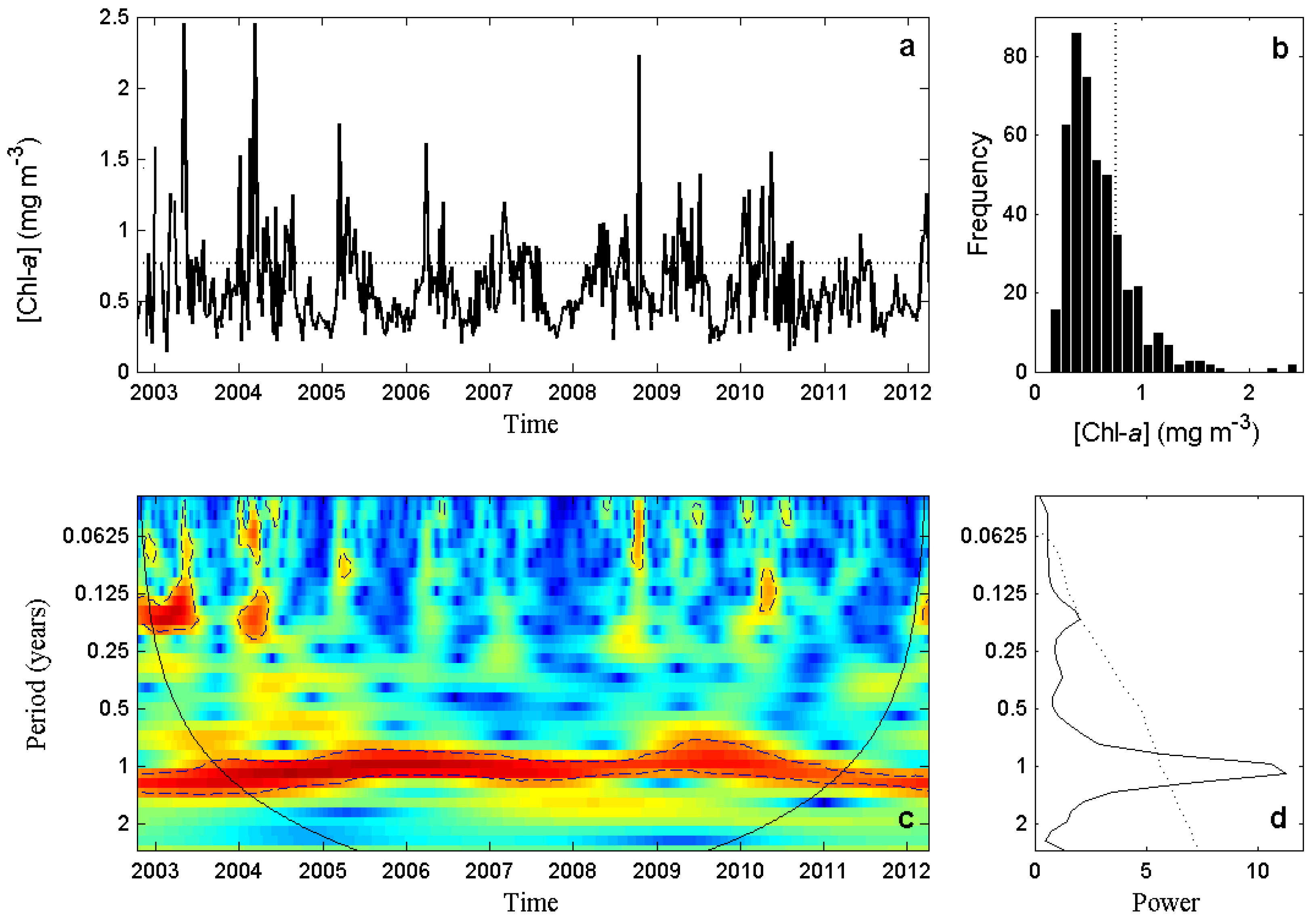
Figure 7.
Analysis of the chlorophyll-a concentration (chl-a; mg m) time series computed for Zone 1. (a) Temporal series of tidal cycle dataset chl-a concentration. (b) Distribution of chl-a concentration. Dotted lines (a,b) show average chl-a concentration. (c) Wavelet power spectrum. Colour code varies from dark blue (low values), to dark red (high values). The black line indicates the cone of influence. (d) Average wavelet power spectrum. Dotted lines (c,d) show the = 5% significance level computed based on 1000 Markov bootstrapped series.
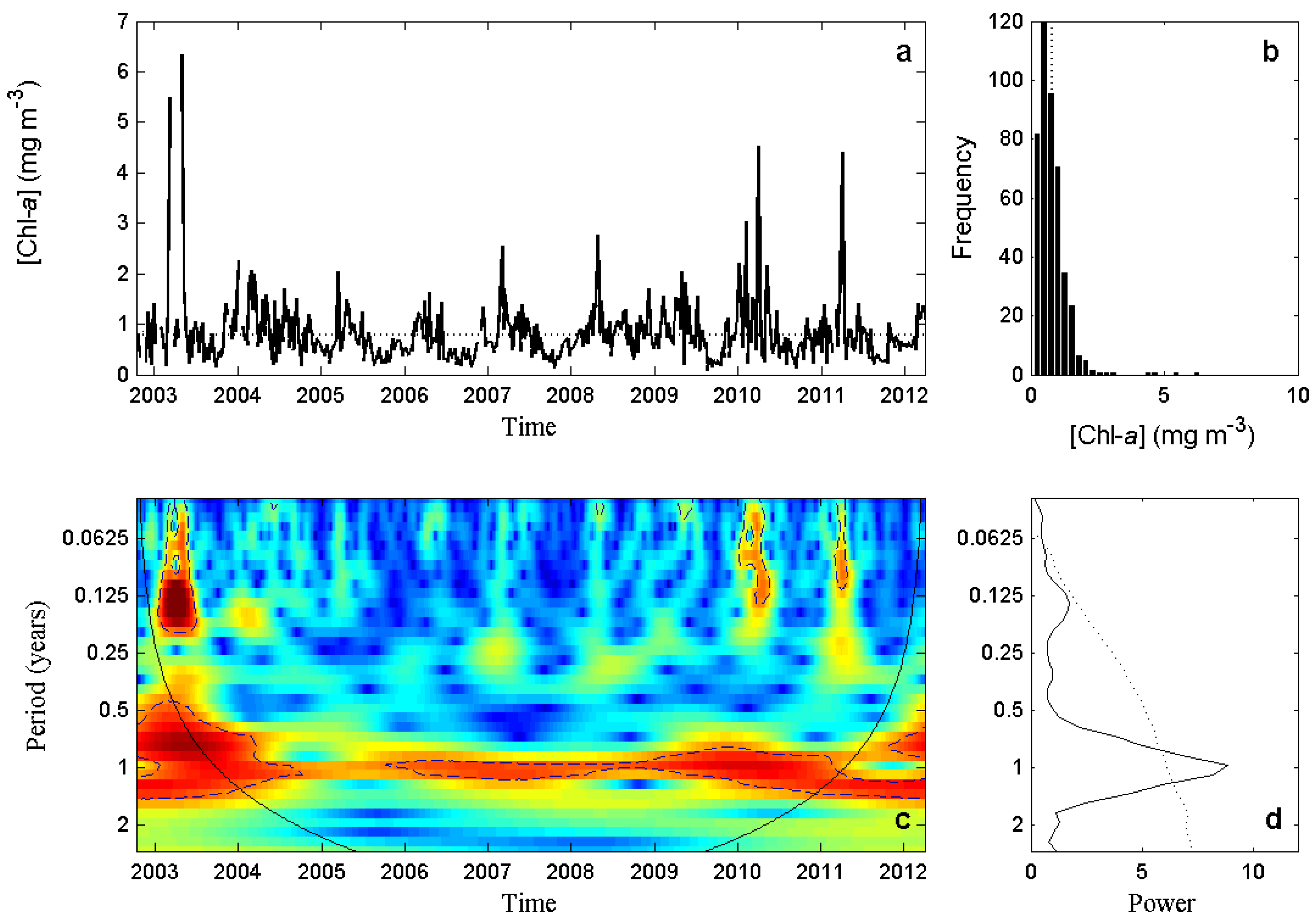
Figure 8.
Analysis of the chlorophyll-a concentration (chl-a; mg m) time series computed for Zone 2. (a) Temporal series of tidal cycle dataset chl-a concentration. (b) Distribution of chl-a concentration. Dotted lines (a,b) show average chl-a concentration. (c) Wavelet power spectrum. The colour code varies from dark blue (low values), to dark red (high values). The black line indicates the cone of influence. (d) Average wavelet power spectrum. Dotted lines (c,d) show the = 5% significance level computed based on 1000 Markov bootstrapped series.

Figure 9.
Left-hand panels: Average wavelet cross-spectrum between chlorophyll-a concentration (chl-a; mg m) and the zonal component of wind (u-wind) in Zone 1 (a) and Zone 2 (c). Dotted lines show the = 5% significance levels computed based on 1000 Markov bootstrapped series. Right-hand panels: Phases of the two time series, chl-a concentration (red line) and u-wind (blue line), computed for the peak of highest coherence in Zone 1 (b) and Zone 2 (d). Dashed lines represent the phase difference between both signals.
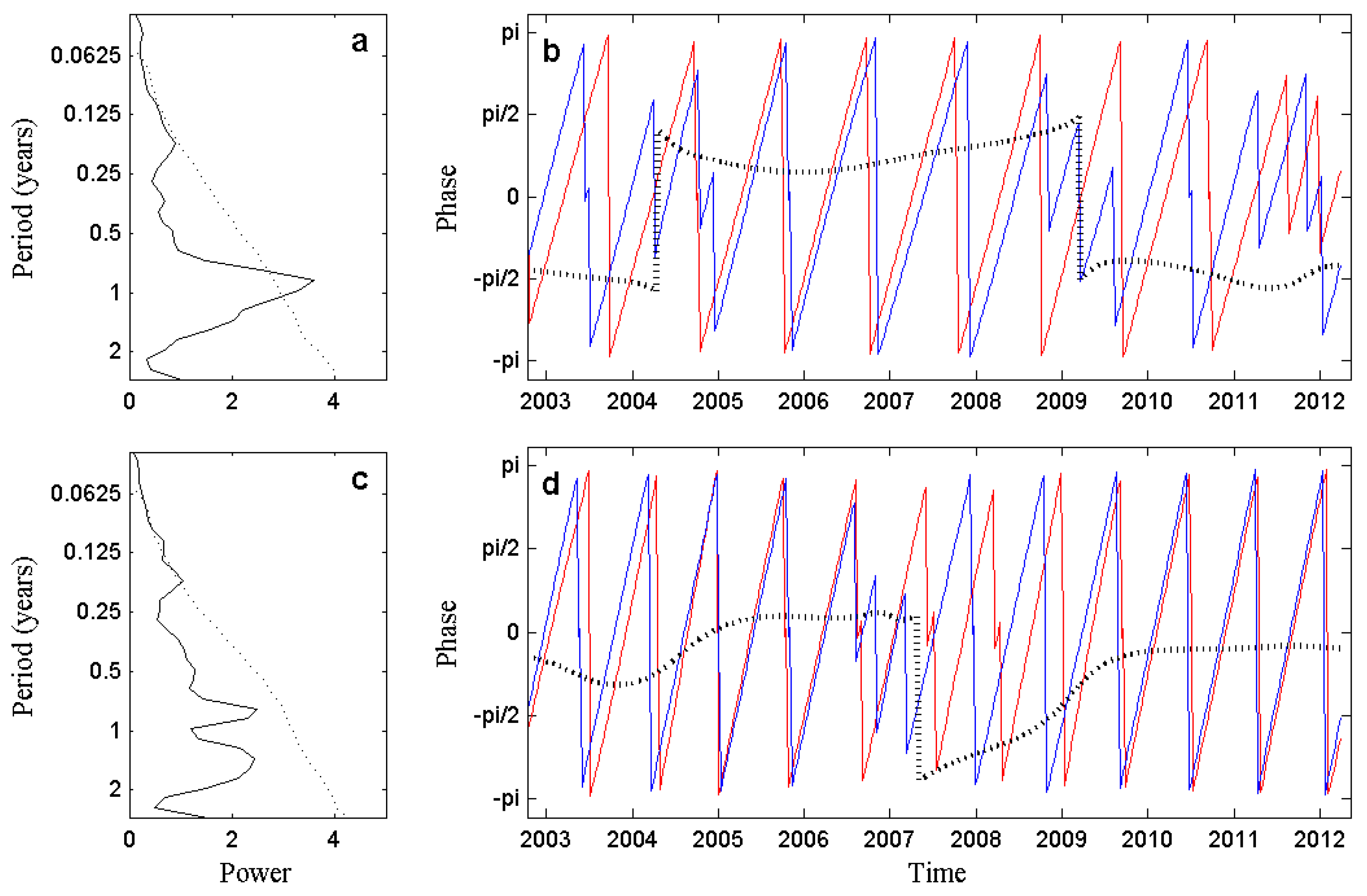
Figure 10.
Left-hand panel: Average wavelet cross-spectrum between chlorophyll-a concentration (chl-a; mg m) and Guadalquivir river discharge in Zone 1 (a) and Zone 2 (c). Dotted lines show the = 5% significance levels computed based on 1000 Markov bootstrapped series. Right-hand panel: Phases of the two time series, chl-a concentration (red line), and river discharge (blue line), computed for the peak of highest coherence in Zone 1 (b) and Zone 2 (d). Dashed lines represent the phase difference between both signals.

Figure 11.
Left-hand panel: Average wavelet cross-spectrum between chlorophyll-a concentration (chl-a; mg m) and zonal component of tidal current (u-tide) for the three selected periods in Zone 1 (a) and Zone 2 (c). Right-hand panel: Phases of the two time series, chl-a concentration (red line), and u-tide (blue line), for the three selected periods, computed for the peak of highest coherence in Zone 1 (b) and Zone 2 (d). Dashed lines represent the phase difference between both signals.


Table 1.
List of L2_flags used in the masking process to assure the quality control of MEdium Resolution Imaging Spectrometer (MERIS) dataset retained for analysis (flags for NASA Level 3-ocean colour processing).
Table 1.
List of L2_flags used in the masking process to assure the quality control of MEdium Resolution Imaging Spectrometer (MERIS) dataset retained for analysis (flags for NASA Level 3-ocean colour processing).
| Flag | Condition |
|---|---|
| LAND | Pixel is over land |
| CLOUD | Cloud contamination |
| ATMFAIL | Atmospheric correction failure |
| HIGLINT | High sun glint |
| HILT | Total radiance above knee |
| HISATZEN | Large satellite zenith |
| CLDICE | Cloud and/or ice |
| COCCOLITH | Coccolithophores detected |
| HISOLZEN | Large solar zenith |
| LOWLW | Very low water-leaving radiance |
| CHLFAIL | Chlorophyll algorithm failure |
| NAVWARN | Questionable navigation |
| MAXAERITER | Maximum iterations of NIR algorithm |
| CHLWARN | Chlorophyll out of range |
| ATMWARN | Atmospheric correction is suspect |
Table 2.
Coherence results between chlorophyll-a concentration and the different environmental variables (zonal component of wind, Guadalquivir river discharge, and zonal component of tidal current). The cycle at which the coherence analysis showed the highest consistency, the power signal for this cycle, and the total variance associated are shown.
| Zonal Component of Wind | |||
| Cycle | Power | Total Variance | |
| Zone 1 | 1 year | ∼3.45 | ∼14.52% |
| Zone 2 | 10 months | ∼2.34 | ∼10.26% |
| Guadalquivir River Discharge | |||
| Cycle | Power | Total Variance | |
| Zone 1 | 1 year | ∼6.94 | ∼18.33% |
| Zone 2 | 10 months | ∼4.88 | ∼11.76% |
| Zonal Component of Tidal Current | |||
| Cycle | Power | Total Variance | |
| Zone 1 | 15 days | ∼10.31 | ∼45.11% |
| Zone 2 | 15 days | ∼5.99 | ∼35.59% |
© 2018 by the authors. Licensee MDPI, Basel, Switzerland. This article is an open access article distributed under the terms and conditions of the Creative Commons Attribution (CC BY) license (http://creativecommons.org/licenses/by/4.0/).
Share and Cite
MDPI and ACS Style
Sala, I.; Navarro, G.; Bolado-Penagos, M.; Echevarría, F.; García, C.M. High-Chlorophyll-Area Assessment Based on Remote Sensing Observations: The Case Study of Cape Trafalgar. Remote Sens. 2018, 10, 165. https://doi.org/10.3390/rs10020165
AMA Style
Sala I, Navarro G, Bolado-Penagos M, Echevarría F, García CM. High-Chlorophyll-Area Assessment Based on Remote Sensing Observations: The Case Study of Cape Trafalgar. Remote Sensing. 2018; 10(2):165. https://doi.org/10.3390/rs10020165
Chicago/Turabian StyleSala, Iria, Gabriel Navarro, Marina Bolado-Penagos, Fidel Echevarría, and Carlos M. García. 2018. "High-Chlorophyll-Area Assessment Based on Remote Sensing Observations: The Case Study of Cape Trafalgar" Remote Sensing 10, no. 2: 165. https://doi.org/10.3390/rs10020165
Note that from the first issue of 2016, this journal uses article numbers instead of page numbers. See further details here.