Article

Estimation of Leaf Area Index in a Mountain Forest of Central Japan with a 30-m Spatial Resolution Based on Landsat Operational Land Imager Imagery: An Application of a Simple Model for Seasonal Monitoring

1
Graduate School of Science, Tohoku University, 6-3, Aramaki Aza-Aoba, Aoba-ku, Sendai 980-8578, Japan
2
River Basin Research Center, Gifu University, 1-1 Yanagido, Gifu 501-1193, Japan
*
Author to whom correspondence should be addressed.
Remote Sens. 2018, 10(2), 179; https://doi.org/10.3390/rs10020179
Submission received: 7 December 2017 / Revised: 19 January 2018 / Accepted: 23 January 2018 / Published: 26 January 2018
(This article belongs to the Section Forest Remote Sensing)

Abstract

:
An accurate estimation of the leaf area index (LAI) by satellite remote sensing is essential for studying the spatial variation of ecosystem structure. The goal of this study was to estimate the spatial variation of LAI over a forested catchment in a mountainous landscape (ca. 60 km2) in central Japan. We used a simple model to estimate LAI using spectral reflectance by adapting the Monsi-Saeki light attenuation theory for satellite remote sensing. First, we applied the model to Landsat Operational Land Imager (OLI) imagery to estimate the spatial variation of LAI in spring and summer. Second, we validated the model’s performance with in situ LAI estimates at four study plots that included deciduous broadleaf, deciduous coniferous, and evergreen coniferous forest types. Pre-processing of the Landsat OLI imagery, including atmospheric correction by elevation-dependent dark object subtraction and Minnaert topographic correction, together with application of the simple model, enabled a satisfactory 30-m spatial resolution estimation of forest LAI with a maximum of 5.5 ± 0.2 for deciduous broadleaf and 5.3 ± 0.2―for evergreen coniferous forest areas. The LAI variation in May (spring) suggested an altitudinal gradient in the degree of leaf expansion, whereas the LAI variation in August (mid-summer) suggested an altitudinal gradient of yearly maximum forest foliage density. This study demonstrated the importance of an accurate estimation of fine-resolution spatial LAI variations for ecological studies in mountainous landscapes, which are characterized by complex terrain and high vegetative heterogeneity.

Graphical Abstract

1. Introduction

Forest ecosystems play an important role in the regulation of the global climate. They are a key component of the carbon cycle because of their large carbon sequestration, heat budget, and hydrological cycle [1]. A major function of forest ecosystems is canopy photosynthesis, determined by multiple factors, including single leaf photosynthetic capacity, meteorological factors (light, humidity, and temperature), and variations of leaf area. In temperate regions, photosynthetic production by forest ecosystems varies seasonally because of the phenology of single leaf photosynthesis and canopy leaf area, and is thus sensitive to climate change [2,3].
Because leaves are the main surface through which energy and mass are exchanged between terrestrial vegetation and the atmosphere, the leaf area index (LAI) is an essential variable used to integrate ecosystem functions such as photosynthesis, transpiration, and autotrophic respiration from the scale of an individual leaf to total tree and canopy scales [4,5,6,7]. LAI is an indicator of forest ecosystem structure, i.e., the geometrical structure and density of foliage. Several definitions of LAI are found in the literature [8,9,10], and the definitions depend on the leaf form (flat or needle) and methods applied for the estimation (true LAI and effective LAI). LAI was first defined by Watson [8] as the total one-sided area of leaf tissue per unit ground surface area. This definition is applicable to flat leaves, both sides of which have the same area. For leaves with other geometries such as needles, Myneni et al. [10] used the term LAI to mean the maximum projected leaf area per unit ground surface area. In this paper, we use the definition of LAI by Myneni et al. [10].
An accurate estimation of the LAI of forest ecosystems is crucial for studies of the structure and function of ecosystems and is required for ecosystem simulation models [11,12,13]. The spatial and temporal variations of LAI are estimated by in situ [4,14] and remote sensing approaches [6,7,15,16,17,18]. The in situ approach consists of direct methods, such as a model tree method, litter-fall collection [4,19,20], and indirect methods, such as contact methods (e.g., inclined point quadrat and allometry [14]) and non-contact optical methods. Optical methods make use of the measurements of PAR transmission through canopies by application of the Monsi-Saeki theory [21]. The Monsi-Saeki theory describes the relationship between the amount of leaves and light penetration in a plant canopy. It states that a total amount of photosynthetically active radiation (PAR), W/m2, intercepted by the canopy, depends on the incident incoming amount of PAR, canopy structure (density of leaves and vertical profile), and leaf optical properties. The equation describing the relationship between PAR-transmittance and amount of leaves (i.e., LAI) of a given plant canopy (Equation (7) in this study) is derived from Beer-Lambert law for the light attenuation in a solution (liquid containing certain concentration of chemical matter). In this study, we use the term “Monsi-Saeki theory” as it is developed for a plant canopy in the original theory. The optical methods include field measurements of light attenuation through the canopy by PAR sensors (namely PAR transmittance), analysis of hemispherical photographs [2,20], or use of commercial instruments [20].
The remote sensing approach is crucial for evaluating spatial variations of LAI over areas from landscape to global scales [16] and includes empirical, semi-empirical, and physical methods. Empirical, or statistical, methods have been used to estimate the spatial variation of LAI based on statistical relationships between LAI and spectral vegetation indices (VIs) derived from passive optical remote sensing imagery. The most frequently used VIs are the normalized difference vegetation index (NDVI), the enhanced vegetation index (EVI), and the soil adjusted vegetation index (SAVI) [6,12,17,18]. While the main advantage of the empirical methods is their simplicity, the passive optical sensors cannot penetrate the dense canopy and obtain the spectral reflectance of the lower canopy and understory. Thus, in high LAI values (LAI ≥ 3), spectral signals, and consequently, LAI–VIs relationships, become saturated [22,23,24]. In addition, VIs are dependent on many factors, such as canopy geometry, leaf and soil optical properties, and sun position [25], which restrict the universal applicability (generality) of the empirical models. Gray and Song [24] have introduced a fine-resolution empirical method for estimating LAI that overcomes the “saturation” limitation by combining image spectral information from Landsat imagery and spatial information from high-resolution panchromatic IKONOS imagery. However, pre-processing of images from multiple sensors increases computational and data requirements, especially in mountainous areas with complex atmospheric and topographic characteristics. In particular, the presence of clouds and aerosols (atmospheric effects) and the shadows of the mountain slopes (topographic effects) lead to a requirement of atmospheric and topographic corrections of each image separately because of the sensor differences in the spectral and spatial resolutions. Above all, if high-resolution imagery is derived with a great off-nadir viewing angle, trees are projected obliquely and cannot be orthorectified without very accurate digital surface elevation models (DEMs).
The physical methods are based on radiative light transfer processes within the canopy, and include radiative transfer modeling, optimization techniques, neural networks, genetic algorithms, Bayesian networks, and look-up tables. Having a firm physical basis, these methods are not restricted to a single plot or biome, and are thus applicable to estimates of LAI over large (up to global) spatial scales [22,24]. The MOD15A2 product of the Moderate Resolution Imaging Spectroradiometer (MODIS) Science Team [15] is among the most frequently used global scale LAI products. It is readily available for the user and has a high temporal resolution (eight days). However, because of the moderate spatial resolution (1 km), MOD15A2 cannot provide a sufficient accuracy required for spatial analysis studies at a landscape scale in the areas of complex terrain. In such areas, topographic and atmospheric characteristics may have a major impact on the ecosystem structure, causing high spatial LAI variation that cannot be resolved by a moderate-resolution imagery pixel size. Furthermore, the reflectance of moderate-resolution imagery, measured with wide field-of-view (FOV) sensors, i.e., MODIS, suffers greatly by bidirectional reflectance characteristics known as the bidirectional reflectance distribution function (BRDF) [26]. Since the correction of bidirectional reflectance characteristics is extremely difficult for mixed forest with different species and BRDFs under rugged terrain, sensors with narrow FOV, i.e., Landsat, have an advantage in deriving accurate reflectance [22]. Thus, for studies at a landscape scale, empirical and semi-empirical methods have been frequently applied to fine-resolution satellite imagery (≤30 m). Fine resolution permits observations of complex and diverse local-scale phenomena, such as land cover changes, deforestation, and growth of vegetation, which have large effects on global carbon dynamics [27].
Landsat mission series (Multispectral Scanner, MSS, Thematic Mapper, TM, Enhanced Thematic Mapper, ETM+ and Operational Land Imager, OLI) provides the world longest continuous globally available fine spatial- (~80 m), temporal- (16 or 18-day revisit), and spectral-resolution imagery, which is, therefore, beneficial for spatially detailed LAI representation compared to moderate-resolution optical satellite imagery. The newest OLI on-board Landsat-8 was launched in 2013 and has several benefits for forest studies compared to its predecessors. First, OLI has a wider dynamic range―higher signal to noise ratio (SNR) and greater (12-bit) quantization than 8 bits of ETM+ [28]. A wide dynamic range is beneficial in the forest studies because of the small reflectance of forest canopies with a narrow digital number (DN) range in visible bands. Landsat OLI can estimate reflectance more accurately than ETM+ because of highly sensitive detectors. Second, the OLI swath width is 185 km (15° FOV from 705 km orbit), which allows vertical (nadir) viewing with a spatial resolution of 30 m per pixel. The reflectance measured with narrow FOV sensors suffers less from BRDF effects. Third, the OLI sensor has a narrower spectral range of the near infrared (NIR) band to exclude water vapor absorption features [28,29]. Thus, OLI imagery involves less atmospheric effects compared to ETM+ and other heritage Landsat sensors. While Landsat products have been widely used to estimate LAI at a landscape scale by the empirical approach [6,12,17,18], very few studies used the benefits of Landsat OLI imagery to estimate spatial variations of forest ecosystem structure and functions [30].
The goal of this study was to estimate the spatial variation of LAI over the forested catchment of a mountainous landscape (ca. 60 km2) in central Japan. For this purpose, we used a simple semi-empirical remote sensing model for estimating LAI based on the Monsi-Saeki theory targeted at densely forested areas. The proposed model benefited from its simplicity and was adaptable for various forest ecosystems. Application of the simple model on the 30-m resolution Landsat OLI imagery allowed spatial analysis in the mountainous area of Japan with high vegetative heterogeneity. Pre-processing of the Landsat OLI imagery was crucial in the area with complex atmospheric and topographic conditions. The complex atmospheric conditions of the study area included high humidity and Mie scattering caused by the yellow sand transported from the Gobi Desert by continental air masses. For atmospheric correction, we applied elevation-dependent dark object subtraction (DOS), which was effective in reducing vertically non-homogeneous atmospheric effects. Minnaert topographic correction diminished the slope shadows in the mountainous landscape, associated with steep topography with an average slope angle of 23° (from approximately 5° to 35°) and the 1000-m elevation gradient (from approximately 600 m above sea level (a.s.l.) to 1600 m a.s.l.).
The present study demonstrated the importance of an accurate estimation of forest LAI in a fine spatial resolution for ecological studies in mountainous landscapes. In particular, we discuss (1) the pre-processing of Landsat OLI imagery for mountainous landscapes; (2) the accuracy of LAI estimations using the simple model; and (3) spatial and temporal variations of LAI in the Daihachiga river basin, with implications for modeling studies aimed at understanding ecosystem structure and functions at a landscape scale.

2. Materials and Methods

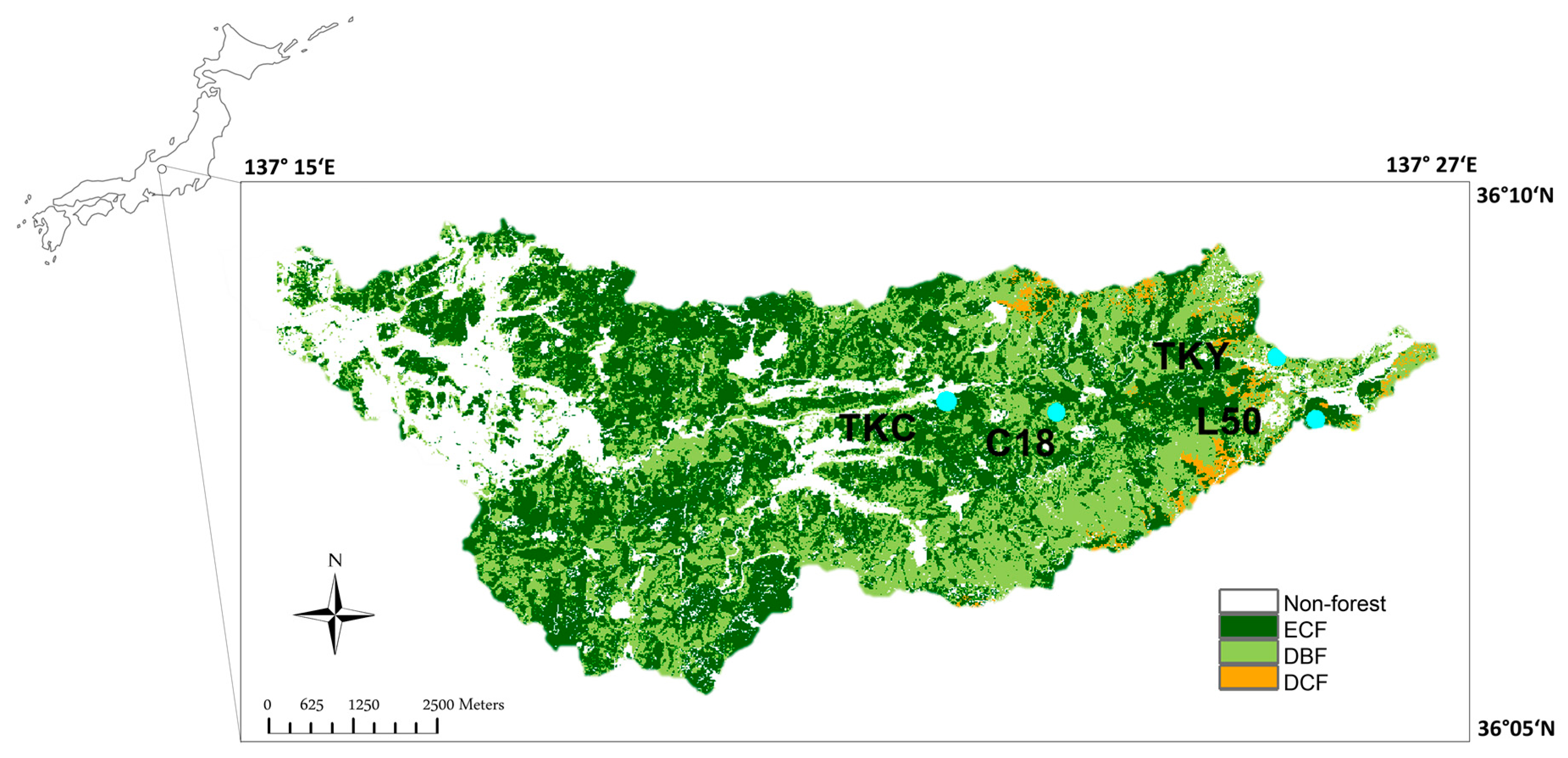
2.1. Study Area and In Situ Measurements

The study area (36°06′ to 36°09′N, 137°15′ to 137°26′E) includes the basin of the Daihachiga River, located on the northwestern side of Mt. Norikura, and comprises the eastern part of the city of Takayama, Japan (Figure 1). The area, which is about 60 km2, has an elevation gradient of 1000 m—from approximately 600 m to 1600 m a.s.l.—and a steep topography [31]. The climate, which is cool and temperate, is influenced by the Asian Monsoon and is characterized by a mild, humid spring and autumn; a hot, humid summer; and a cold, snowy winter [32]. The study area includes various forests—deciduous broadleaf forests (DBFs), deciduous coniferous forests (DCFs), and evergreen coniferous forests (ECFs)—paddy fields, and urban areas [31,33].
An in situ estimation of LAI was carried out at four study plots, which included three different forest types within the study area (see Table 1 for detailed descriptions). Two of the plots, TKY (Takayama Flux Site) and TKC (Takayama Evergreen Coniferous Site), are both part of three research networks—the AsiaFlux network (http://www.asiaflux.net/), the Japan Long–Term Ecological Research network (JaLTER, http://www.jalter.org), and the Phenological Eyes Network (PEN, http://www.pheno-eye.org). C18 and L50 are ecological research plots, which were established in 2004 as a part of the Satellite Ecology (SATECO) project [34]. C18 is covered by young secondary mixed forest, dominated by coppice chestnut and oak after clear-cutting in the autumn of 1986 [35], while its primary climax vegetation was a cool-temperate deciduous broadleaved forest, dominated by Japanese beech (Fagus crenata) and oak (Quercus crispula). L50 is a study plot located in a gentle slope (10–15°) within a 2 km distance from TKY. It is dominated by the only deciduous coniferous forest species in Japan, Japanese larch (Larix kaempferi), and has several broadleaf deciduous species in the understory.
In situ LAI estimates were used to validate the performance of the simple LAI model on the Landsat OLI imagery (spring and summer maximum LAI during 2013). The methods for LAI estimation at the four study plots were based on data availability (Appendix A): either litter-fall collection (at C18 and TKY), PAR transmittance (at TKY), or allometry (at L50 and TKC). Because LAI is a dynamic variable that has a defined phenology in forests, in situ estimation of the LAI seasonal profile was necessary to validate the simple model estimates of spring LAI variations. Unlike PAR transmittance, the application of methods such as litter-fall collection and allometry does not provide a complete seasonal profile of LAI variations, giving little or no information about LAI during the leaf-expansion period [4]. Therefore, we examined leaf seasonality at the deciduous plots (DBF and DCF) making use of the available PAR transmittance-based LAI estimates at TKY and the dependency of LAI phenology on the air temperature during the growing season. We only examined LAI seasonality at three deciduous forest sites, because in the previous study, Saitoh et al. [32] showed that LAI has little seasonality at TKC (an ECF study plot). In temperate deciduous forest areas, LAI increases in spring because of warmer air temperatures and reaches its maximum in the middle of summer following the phenological cycle of the ecosystem. Hence, the rate of the spring LAI increase depends on the air temperature during the growing season that can be described by the cumulative effective temperature (CET), °C, according to:
C E T k ( t ) = i = 1 t max ( T i k , 0 ) ,
where t is time (day of year, DOY); Ti is the daily mean air temperature on DOY i; and k is a base threshold temperature, °C, for temperature accumulation. To estimate the seasonal LAI of deciduous forests, we implemented an empirical in situ logistic model [38,39] that describes the seasonal variations of LAI as a function, f(x), of the CET > 2 °C at a daily time step,
f ( x ) = a + b 1 + exp ( c d x ) ,
where x = CET2, a, b, c, and d are dimensionless parameters: a and b control the lower and upper limit of the function, where (a + b) is the maximum LAI, parameter c causes parallel shifts in response to the driving variable x , and parameter d affects the rate of change of f( x ). Parameters a, b, and d are non-negative, and c is positive in the leaf-expansion and negative in leaf-senescence periods [38].
The above logistic model was based on field measurements at TKY, which has been an intensive multi-year observational station for carbon cycle research [2] (Figure 2). Results yielded a = 0.10, b = 5.94, c = 5.16, and d = 0.01. The logistic model was then adjusted for two other deciduous forest study plots using the maximum LAI estimated via the litter-fall collection and allometric equations at C18 and L50, respectively. Daily mean air temperature at each study plot for the model was estimated from the temperature lapse rate, which is a decrease of air temperature with altitude. We used the annual mean air temperature at four study plots to check the linear dependency of air temperature on the altitude and obtained a lapse rate of 7.00 °C/km.

2.2. Pre-Processing of Satellite Imagery

Because the Landsat OLI has a 30-m spatial resolution and enhanced spectral performance (compared to its predecessors MSS, TM, or ETM+), it can improve the accuracy of ecosystem structure estimations at a landscape scale. However, the Landsat missions provide raw spectral reflectance, which may include atmospheric and topographic effects (distortions). Pre-processing of the imagery is therefore essential to obtain accurate estimates of LAI. We selected four Landsat OLI images (path 109, row 35) with the smallest possible cloud cover for the seasonal spatial analysis (Table 2). The imagery was downloaded from the Earth Resources Observation and Science Center, United States Geological Survey, USGS, (http://glovis.usgs.gov/). Because only visible and near-infrared spectra were required for the proposed LAI model, only OLI bands 2–5 were pre-processed.
We prepared the Landsat OLI sub-images (Figure 3), which included the Daihachiga river basin, a dam (a clear, dark object for atmospheric correction), and a large parking lot (for validation of topographic correction). The area covered by Landsat OLI sub-images, had an elevation gradient of 2700 m—from approximately 500 m to 3200 m a.s.l. Besides the Landsat OLI imagery, we used a DEM with s 30-m resolution distributed by The Geospatial Information Authority of Japan, land cover map with a 2-m resolution, based on LiDAR and Quickbird imagery obtained in 2007 [33], and an aerial composite photograph with a 0.5-m resolution, provided by the Gifu Prefecture government. The DEM was resampled to 30 m from 1-m resolution DEM, produced by an airborne laser measurement on the Japan Plane Rectangular Coordinate System (CS) VII with Japanese Geodetic Datum (JGD) 2000. Therefore, the horizontal and altitudinal accuracy of DEM was very high.
To spatially align remote sensing data and relate it to in situ LAI estimations, we transformed Landsat OLI imagery to the Japan Plane Rectangular CS VII with JGD 2000. However, because OLI images were re-projected after the measurements at least twice (first, by USGS team to Universal Transverse Mercator map projection with World Geodetic System 84), some level of discrepancy with the geographical location or DEM might exist. It probably leads to minor errors in topographic correction and, therefore, LAI estimation; however, this is not significant in the spatial analysis over a large area.
The Landsat OLI sub-images underwent pre-processing, namely atmospheric (Section 2.2.1.) and topographic (Section 2.2.2.) corrections using the software ERDAS Imagine ver. 2015, (ERDAS Inc., Norcross, GA, USA), ArcMap 10 (ESRI, Redlands, CA, USA), and QGIS (Quantum GIS Development Team, 2014). SYSTAT 13 software (Systat Software, San Jose, CA, USA) was used for the statistical analysis. LAI estimations based on spring imagery (26 May 2013 and 18 May 2016) were used for the analysis of spatial variations of leaf expansion timing. LAI estimations based on summer imagery (14 August 2013 and 4 August 2015) were used for the analysis of spatial variations of summer maximum LAI.

2.2.1. Atmospheric Correction

The satellite imagery of the study area was strongly affected by vertically non-homogeneous atmospheric scattering and, therefore, required careful atmospheric correction. Strong atmospheric conditions were induced by high humidity (climate of central Japan is characterized by humid spring and summer), the seasonal variation of scattering effects (the monsoonal circulation leads to prevailing Mie and Rayleigh scattering in the first and second half of the year, respectively), and a large altitudinal gradient in the mountainous terrain (the optical depth decreases with elevation) [30,40]. To atmospherically correct the OLI imagery, we implemented an empirical algorithm, elevation-dependent DOS [30]. This method stems from classical DOS [41] based on the assumption that at least a few pixels within a satellite image (like deep clear water) have zero reflectance (and DN). As these pixels supposedly represent atmospheric scattering, they will not appear absolutely dark. The resulting nonzero value of the pixel should be subtracted from DNs. The DOS method has a great advantage because it is established solely on the imagery with no requirement of ground measurements. Unlike the classical algorithm, the elevation-dependent DOS assumes the presence of the dark object in each selected altitudinal range. Therefore, it can correct for elevation (altitude)-dependent differences in atmospheric effects, which to the best of our knowledge, neither classical DOS nor available commercial software for atmospheric correction would correct.
The elevation-dependent DOS [30] uses the Equation (3)
D N D O S = D N R A W ( t + s × DEM ) + O f f s e t 1 ,
where DNDOS and DNRAW are the atmospherically corrected DN and original DN, respectively; Offset1 denotes the offset DN for correction of negative DN values; DEM denotes the ground elevation; and t and s are the intercept and slope of the regression of minimum DN on the ground elevation, respectively.
We extracted the minimum (MIN) DN of each 100-m altitudinal zone from 500 m to 3200 m a.s.l., checked the pixels using aerial photographs, and calculated linear regressions of MIN DN versus elevation for visible OLI bands (Table 3). For spectral band 5, the relationship between elevation and MIN DN could not be determined because of the large variation of the reflectance of dark objects in the NIR range. We therefore applied the DOS for all the sub-images by subtracting a constant MIN DN of the selected dark object—lake water [41]. After implementation of the atmospheric correction, DNs were converted into reflectance factors (RFs) with Equation (4):
R F A = M ρ D N D O S   ×   sin θ z ,
where RFA is the atmospherically corrected RF, Mρ is the band-specific multiplicative rescaling factor from the metadata (which was 2 × 10⁻⁵ in all cases of the present study), and θz denotes the sun elevation angle [42].
For validation of the atmospheric correction, we used the fact that the reflectance of dense, dark coniferous forest pixels is low in the visible spectrum [43] and stable along an altitudinal gradient. Therefore, using the aerial photographs, we selected seven pixels of the dense, dark ECF at different altitudes. The atmospherically corrected reflectance was compared with the reflectance of Norway spruce measured via a helicopter-borne spectrometer by Williams [44] on the assumption that the spectral reflectance of the dense, dark coniferous forest (both Norway spruce and Japanese cedar) can be used as the equivalent of dark objects controls [45]. The elevation-dependent DOS resulted in overcorrection of the visible spectrum (disappearance of the green peak in the vegetation pixels). The overcorrection was constrained by an additional offset RF (Table 4).

2.2.2. Topographic Correction

The topographic features of the study area with an average slope angle of 23° appeared darker and brighter because of the dependence of the shading effects on the orientation of the slopes to the sun. We applied the Minnaert topographic correction, a method that accounts for non-Lambertian surfaces and makes use of the empirically developed, wavelength-dependent Minnaert constants [46,47,48]. Atmospherically corrected reflectances for bands 2–5 were therefore adjusted for topographic effects using Equation (5) [46]:
R F H = R F T ( c o s θ z cos i ) K k ,
where RFH is the topographically corrected reflectance (of a horizontal surface), RFT is the given reflectance of an inclined surface, i is the solar incidence angle, θZ is the solar zenith angle and Kk is the Minnaert constant for band k. The pixels used to compute the Minnaert constants were extracted from the areas of mixed forest. The areas were examined visually using aerial photographs and a moving window of 3 × 3 pixels in order to choose only pixels with low standard deviations. Using this approach, we extracted 263, 189, 271, and 321 pixel samples from the Landsat OLI sub-images dated 26 May 2013, 14 August 2013, 4 August 2015, and 18 May 2016, respectively.
The main shortcoming of the chosen topographic correction method was overcorrection in the steep, shaded slopes [48]. However, no further procedure for removing the residual topographic effects was implemented on the assumption that minor local effects would not significantly influence the spatial analysis over a large area. The pre-processed Landsat OLI reflectance (bands 2–5) was applied in the LAI model.

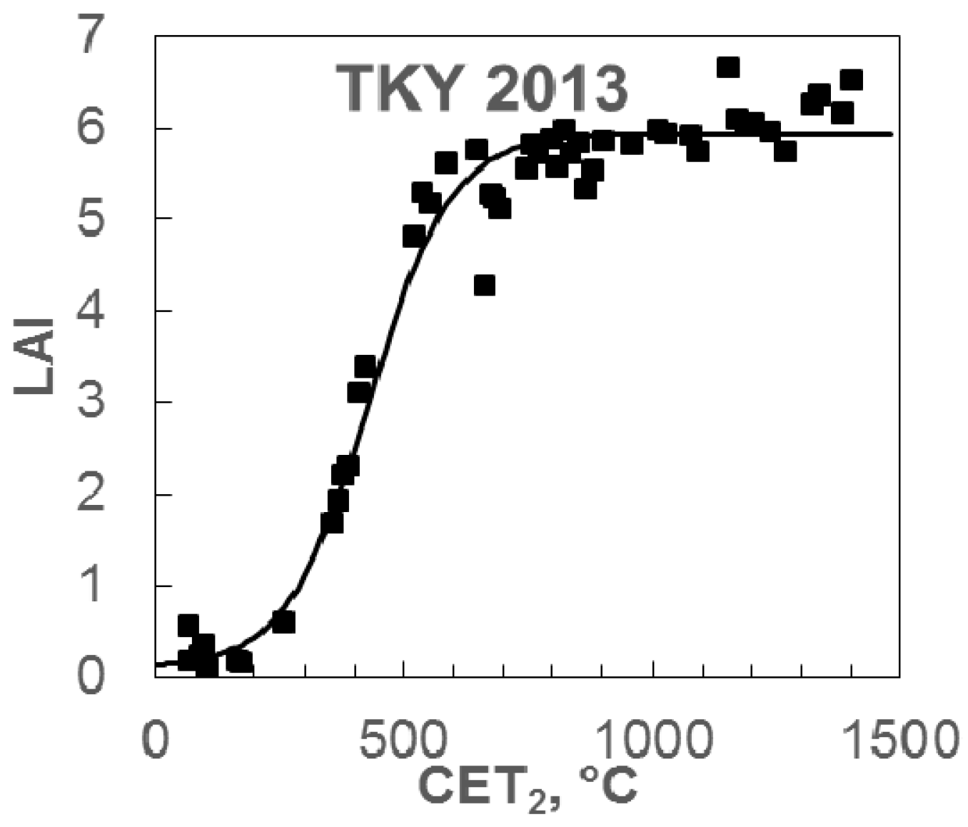
2.3. Leaf Area Index Model

The simple LAI model used in the present study was developed by Awaya et al. [49] and was used to map the seasonal LAI over Japan using MODIS imagery. The model implicates the Monsi-Saeki theory, which describes the relationship between the amount of leaves and light penetration in a canopy [21]. The theory states that light intensity decreases exponentially through the leaf layers according to the Beer-Lambert law on the assumption of the random spatial distribution of leaves. Light, i.e., PAR, W/m2, transmitted through the canopy, can be computed by following Equation (6):
P A R t = P A R 0 e k L A I ,
where PAR0 is the downward PAR reaching the forest canopy top, PARt is the PAR transmitted through the canopy, and k is a dimensionless extinction coefficient of light attenuation defined for each forest type. To estimate LAI, the Equation (6) is modified to:
LAI = k 1 ln ( P A R t / P A R 0 ) .
The Monsi-Saeki theory is widely used in ecological LAI estimation methods, particularly in situ indirect optical methods, i.e., PAR transmittance. Because the approach does not distinguish photosynthetically active leaf tissue from other plant elements (stem, branches), LAI estimated by applying the Monsi-Saeki theory is termed effective LAI [20,50].
Adapting the theory for optical remote sensing, the simple model assumes that the PAR that reaches the canopy is divided into components that are transmitted, absorbed, or reflected by the canopy and ground. Thus, a fraction of absorbed PAR (ƒAPAR), a variable controlling the photosynthetic activity of plants, can be determined according to Equation (8):
ƒ APAR =   P A R 0     P A R r     P A R t     P A R g P A R 0 ,
where PARr is the PAR reflected by the canopy, PARg is is the PARt reflected from the ground.
In the plant communities, where chlorophyll absorption dominates the optical properties, transmitted and reflected PAR (PARt and PARr) are very low (only about a few percent of PAR0), while PARa is high [44]. In the areas of dense vegetation (forests) specifically, PARt is extremely low (at most 1%) [51] and soil reflectance is generally about 15–30% of PARt [22]. Thus, PARg is less than 0.3% of PAR0 (in the visible spectrum). Consequently, because PARg in the areas of dense vegetation cannot be derived or estimated by satellite remote sensing, the simple LAI model assumes that PARg from Equation (8) is very small and negligible in the forests. This assumption restricts the application of the simple model to closed canopies. The model cannot be applied in areas of sparse vegetation, where PARg (i.e., bright sandy soil) can be more than 30% of PAR0.
Commonly, ƒAPAR is estimated as a linear or nonlinear function of the NDVI [49,52,53,54]. Therefore, we assumed the linear NDVI–ƒAPAR relationship to find the fraction of transmitted PAR:
P A R t P A R 0 =   1 P A R r P A R 0 ( a × N D V I + c ) ,
where a and c are the dimensionless slope and intercept of a linear regression between NDVI and ƒAPAR. In remote sensing, a fraction of reflected PAR can be described as reflectance of the visible spectrum (average reflectance of blue, green, and red spectral Landsat OLI bands). Therefore, the equation fraction of transmitted PAR is modified to:
P A R t P A R 0 =   1 V I S ( a × N D V I + c ) ,
where VIS is a reflectance of the visible spectrum. A combination of Equations (7) and (10) gives a final formulation of the simple model:
LAI = k 1 ln [ ( 1 V I S ) ( a × N D V I + c ) ] .
In order to apply the simple LAI model to the Landsat OLI imagery of the Daihachiga river basin, we made several adaptations. First, we used in situ derived extinction coefficients and empirical NDVI–ƒAPAR regression. We selected the empirically derived simple linear regression, developed by Inoue and Olioso [53], from airborne remote sensing imagery of 107 different plant canopies, such as crop fields (e.g., rice, soybean, corn, peanut, etc.) and natural vegetation areas (e.g., tree, turf grass, bush, etc.), for two years (r2 = 0.84). We estimated that a and c in Equation (11) are equal to 1.176 and −0.145, respectively. Second, we determined values of k for the three forest types in the study area (DBF, DCF, and ECF) on the assumption that k was constant throughout the growing seasons [55]. Extinction coefficients for DBF and DCF study plots were taken from the published literature [4,56]. Specifically, for the DBF, we used k = 0.46, a value derived from a direct in situ LAI estimation at TKY [4]. For the DCF, we used k = 0.58, a value derived from the estimated plant area index (PAI) and the attenuation of diffuse solar radiation through the canopy [56]. PAI, which is defined as the aboveground plant area per unit ground surface area [4,5], accounts for both the leaves and woody parts of a tree (stems and branches) and can be derived from Equation (12):
PAI = LAI + WAI ,
where WAI is the wood area index. Because the applied to DCF extinction coefficient was originally developed for PAI, we subtracted WAI to determine the value of LAI after the simple model estimated PAI. We used a constant WAI = 1.4, which was determined for a Japanese larch forest in Tomakomai, Hokkaido, Japan [56]. The extinction coefficient of 0.41 for the ECF was determined from the maximum LAI, which we estimated using the PAR transmittance method, PAR measurements at TKC in 2006, LMA, and allometry-based LAI (Appendix A).

3. Results

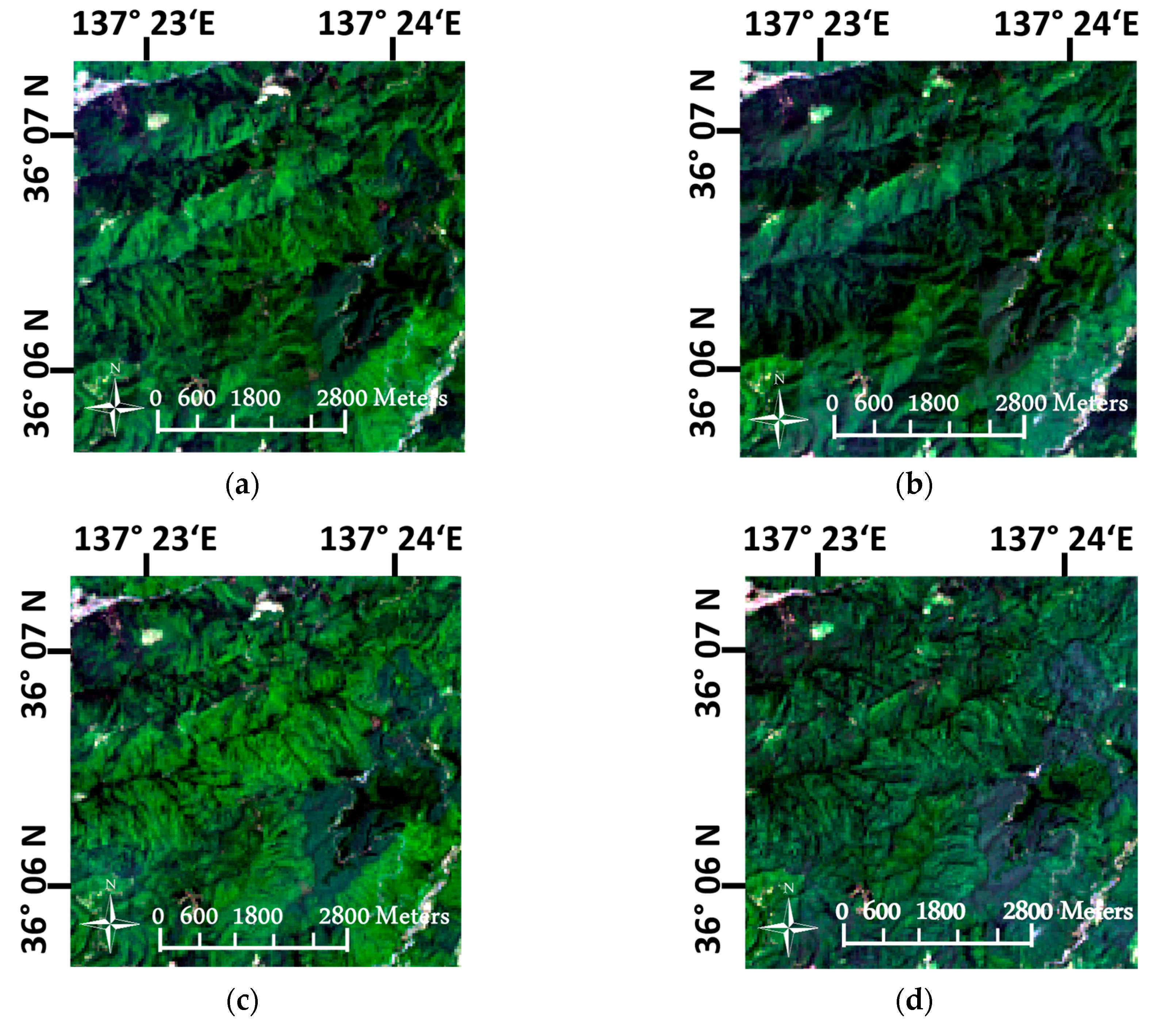
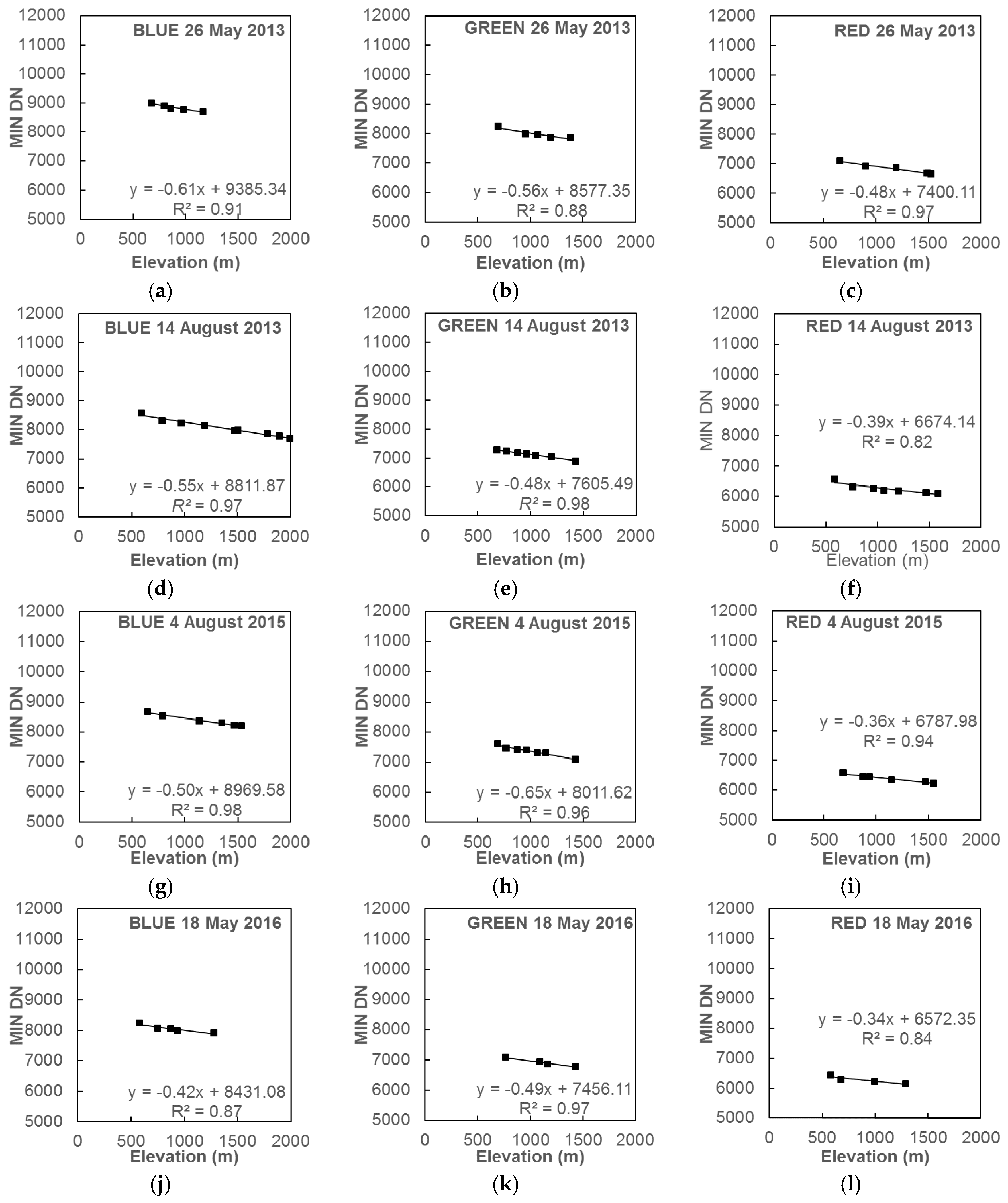
3.1. Pre-Processing of Landsat OLI Imagery

Application of elevation-dependent DOS on the Landsat OLI imagery efficiently reduced the effects of overall atmospheric scattering and variation of optical depth along an altitudinal gradient (Figure 4). Examination of the dark objects pixel-by-pixel in each 100-m altitudinal zone using aerial photographs was necessary to determine reliable linear regressions of atmospheric effects on altitude (Appendix B). The path radiance appeared clearly wavelength-dependent, the highest values being in band 2 (up to 8%) and gradually decreasing at longer wavelengths. Among four sub-images, 26 May 2013 had the strongest atmospheric effects: relatively large cloud coverage was concomitant with two visible aircraft contrails 30 km from the Daihachiga river basin, an indication of humid atmospheric conditions with a large amount of water vapor, in addition to a Mie atmosphere, typical for the main islands of Japan in spring. The applied DOS method corrected for vertically non-homogeneous atmospheric conditions and thereby caused the elevation-dependent difference in reflectance to disappear.
The Minnaert correction method was effective in removing most of the slope shadows in the mountainous terrain (Figure 5). The major topographic features were no longer apparent, although a few shadows could still be detected. For successful implementation of the topographic correction, the selection of pure-pixel samples of the mixed forest randomly distributed in the study area was crucial. The effectiveness of the topographic correction was especially notable in two August sub-images because of the relatively low solar elevation and, consequently, stronger shadow effects in the mountainous landscape.

3.2. LAI Model Performance and Validation

Validation of the simple model involved the in situ LAI estimates of 26 May 2013 (spring) and 14 August 2013 (maximum summer) at four study plots (Table 5). Summer in situ LAI was higher at the two coniferous forest study plots, where it was estimated using the allometric equations for the determination of dry leaf litter mass. Because ECF underwent only a slight seasonal variation [32], LAI at TKC was assumed constant throughout the season. In the cool-temperate Takayama area, leaf expansion generally occurred in the middle of May, foliage density (leaf area) matured in late June, and leaf fall occurred in October [3]. At the two other deciduous forest plots (C18 and L50), which were located at lower altitudes than TKY, leaf expansion was projected to occur earlier in the spring.
Of the three applied methods, the PAR transmittance (indirect optical) method estimated effective LAI, whereas the litter-fall collection (direct contact) method and allometry (indirect contact) method estimated the true LAI. Because the LMA is site- and species-specific [4], estimation errors may be caused by inaccurate LMA values used in Equation (A1). Whereas the LMA at TKY was derived directly from in situ leaf measurements [4], the LMA at C18 was assumed to be equal the LMA at TKY, and LMA at L50 was taken from the published literature [57].
Figure 6 shows estimations of the LAI spatial variation at a spatial resolution of 30 m by the simple model (this study) and at a spatial resolution of 1000 m by the MOD15A2 product. The MOD15A2 could not represent the LAI variation, which was very much affected by heterogeneous vegetation and topographic features smaller than the MODIS product pixel size. The mean maximum LAI of four sub-images was 5.0 ± 0.1, with a maximum of 5.5 ± 0.2 for DBF (1000–1100 m a.s.l.) and 5.3 ± 0.2 for ECF (1100–1200 m a.s.l.) estimated on 14 August 2013. Whereas the mean maximum LAI along an altitudinal gradient was higher in the DBF areas, the mean average LAI was higher in ECF areas. LAI values of both DBF and ECF are the highest in summer.
Figure 7 shows the results of the in situ validation of the estimations on 26 May 2013 and 14 August 2013. The validation procedure verified an adequate performance of the simple LAI model at DBF plots, but the model underestimated the LAI in ECF and DCF areas. The model-based LAI was seasonally and interannually stable within the range 2.7–3.3 at L50 and 4.3–5.4 at TKC during the study period. The largest underestimation occurred in the DCF areas.
Because the model performed best in the DBF areas, we present the spatial analysis solely for that forest type. We derived average LAI values from all DBF pixels (N = 59,075) within the altitudinal range 600–1600 m a.s.l. in the Daihachiga river basin (Figure 8). The maximum spatial average LAI, regardless of seasonality, was consistently in the 800–1100 m a.s.l. range and decreased at lower and higher altitudes. The LAI decrease in May was more apparent than in August because of leaf seasonality (in spring). Both the maximum summer LAI and leaf expansion timing thus appeared dependent on elevation, and LAI therefore decreased with increasing altitude in the mountains. The summer maximum LAI in 2015 appeared lower than in 2013 along the altitudinal gradient, and the LAI was lower on 26 May 2013 than on 18 May 2013. The LAI of the DBF at altitudes of 700–1200 m a.s.l. on 26 May 2013 was as much as 83–85% of the maximum LAI for the year 2013 and gradually decreased at higher altitudes. Although a LAI increase up to altitudes of ca. 1000 m a.s.l. was consistently observed in all Landsat OLI imagery, decreases at altitudes >1000 m a.s.l. were more apparent in spring, the time of leaf expansion, concomitant with temperature decreases at high altitudes.

4. Discussion

4.1. Imagery Pre-Processing in the Mountainous Landscape

The pre-processing of satellite imagery in areas of complex terrain with vertically non-homogeneous atmospheric conditions remains challenging. A method that uses ground-truth information is the most accurate in terms of correcting for atmospheric scattering effects. However, such data are usually difficult to access [17,41,58,59]. Therefore, DOS methods based on the assumption that at least one pixel in an image is a perfect solar radiation absorber (i.e., completely black) are frequently implemented [41]. The elevation-dependent DOS is an appropriate option for regions with complex topography and large variations of optical depth along the altitudinal gradient [45]. The advantage of the proposed atmospheric correction method is its applicability to complex terrains with strong Mie scattering and water vapor effects. Being based completely on satellite imagery, the elevation-dependent DOS does not require any additional ground-based parameters. In addition, the selection of Landsat OLI imagery with higher SNR compared to heritage Landsat sensors allowed us to determine the relationship between elevation and dark objects more accurately.
Although the proposed atmospheric correction method evidenced an ability to correct for vertically non-homogeneous atmospheric effects, the approach did not include systematic ground validation. Because there was no ground validation to confirm the accuracy of the atmospheric corrections, the corrected spectral reflectance of dense, dark Japanese cedar was associated with the published reflectance of Norway spruce [44] on the assumption that the two species are equivalent dark-object controls. Hence, some level of uncertainty related to the reflectance equivalence of the two different types of dark, dense ECF remains in the proposed pre-processing procedure.

4.2. Accuracy of Leaf Area Index Estimation by the Simple LAI Model

The simple model underestimated LAI in areas of coniferous forest—DBF to a greater extent than ECF (Figure 7). The reason for the underestimation by the model might be related to the differences in LAI estimation methods used in the study. In situ LAI at the two coniferous plots was estimated by the direct, non-contact method (e.g., litter-fall collection), which leads to an estimate of the true LAI [60]. Indirect LAI estimation methods involve measurements of radiation transmission through the canopy [20] and lead to estimations of the effective LAI [50], which, without an applied correction, involves clumping effects of the needles and shoots. The effective LAI is more closely related to vegetated surface reflectance [60]. The true LAI may be 1.5 times the effective LAI in coniferous stands [13]. Consequently, because satellite imagery does not distinguish between wooden and photosynthetic canopy parts, but instead records only the reflectance of the canopy roughness [7], the in situ effective LAI is better correlated with the remote-sensing-based LAI. In fact, Saitoh et al. [32] estimated the PAI at TKC as 4.9 and 5.2 in 2006 and 2007, respectively, via the PAR transmittance method [28], a result consistent with the simple-model-estimated LAI reported here.
In situ validation is critical for the estimation of LAI based on satellite imagery. In situ direct contact methods are recognized as the most accurate and are frequently used as a reference tool for indirect estimation methods [20]. However, regardless of the many advantages of in situ direct contact methods, there is no guarantee of their accuracy. Litter-fall collection can considerably miscalculate LAI if the litter traps are affected by winds [61]. The method is not appropriate for estimating a full time series of LAI during a growing season in deciduous forests because it provides little information about LAI during the leaf-expansion stage [4]. In addition, litter-fall collection is not suitable for ECF stands, where the phenology is not clearly defined. Alternatively, indirect methods do not account for foliage clumping [20] that makes derivation of the true LAI unmanageable. As a result, LAI estimated by PAR transmittance is not correlated with LAI estimated by direct methods [62]. This discrepancy arises from differences in the assumptions that the methods make regarding the geometrical features of the canopy—methods that estimate the true LAI assume a horizontal display of leaves, whereas methods that estimate the effective LAI assume a heterogeneous distribution of leaves with differing inclination angles. This inconsistency between the in situ LAI estimation methods accounts for the discrepancy in the validation results in areas with heterogeneous vegetation.
The in situ validation of the model was restricted to the limited number of study plots. Because in this study only four plots were available, there was a large discrepancy between Landsat and in situ LAI estimates. Although the selected plots could represent the variety of forest types in the area, a larger number of plots, and consequently, a larger validation area, is necessary to increase the reliability of the model. Thus, the next step to validate the accuracy and improve the simple model would be creating a larger sample of study plots with a sampling strategy designed by taking into account the seasonal, areal, tree size, and tree density distribution.
The extinction coefficient used in the DCF study (the L50 plot) was originally derived from PAI [56]. To estimate LAI, a constant value of WAI was therefore subtracted from the model-derived LAI. Hirata et al. [56] have estimated the effective LAI estimated by indirect methods to be about 70% of the values derived from the litter-fall collection method. The difference explains the constant underestimation of LAI in the DCF area. In future studies, the relationship between PAI and the effective LAI should be explored more thoroughly. Similarly, because the light extinction coefficient is greater for PAI than for LAI [63], substitution of the relevant coefficients should be done with caution. Several studies [3,54] have suggested that the relationship between photosynthetic parameters and canopy reflectance follows a seasonal pattern and that there is a difference between the green-up and senescence periods. Development of the forest type- and season-dependent relationships between NDVI and ƒAPAR for the LAI model would further improve the model’s performance.
Although the present model is restricted to dense vegetation, it has important advantages compared to existing remote sensing LAI estimation models. First, because the simple model uses a linear NDVI–ƒAPAR rather than curvilinear VI–LAI relationship (with saturation in high LAI values), it is easier to identify the accuracy of the model performance. Second, compared to empirical approaches [17,24,64], the proposed semi-empirical model mainly relies on the Beer-Lambert law (Monsi-Saeki theory) rather than site-specific VI–LAI relationships. In addition, Inoue and Olioso [53] showed that the linear NDVI–ƒAPAR relationship (used in the model) holds among various plants such as crops and tree species. Therefore, the LAI estimation model is adaptable for various forest ecosystems by changing the extinction coefficient, which can be selected for various ecosystems from numerous present in situ studies [4,56]. Unlike physical approaches [15,65], the proposed model benefits from its simplicity and need for only a few input parameters. Consequently, it is suitable for studies over a large range of geographical areas and spatial scales from forest catchment to sub-continental [49].

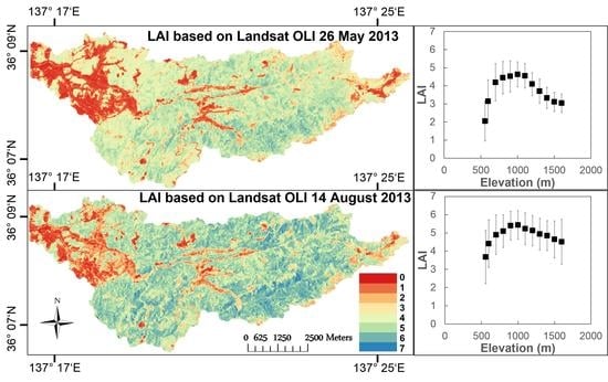
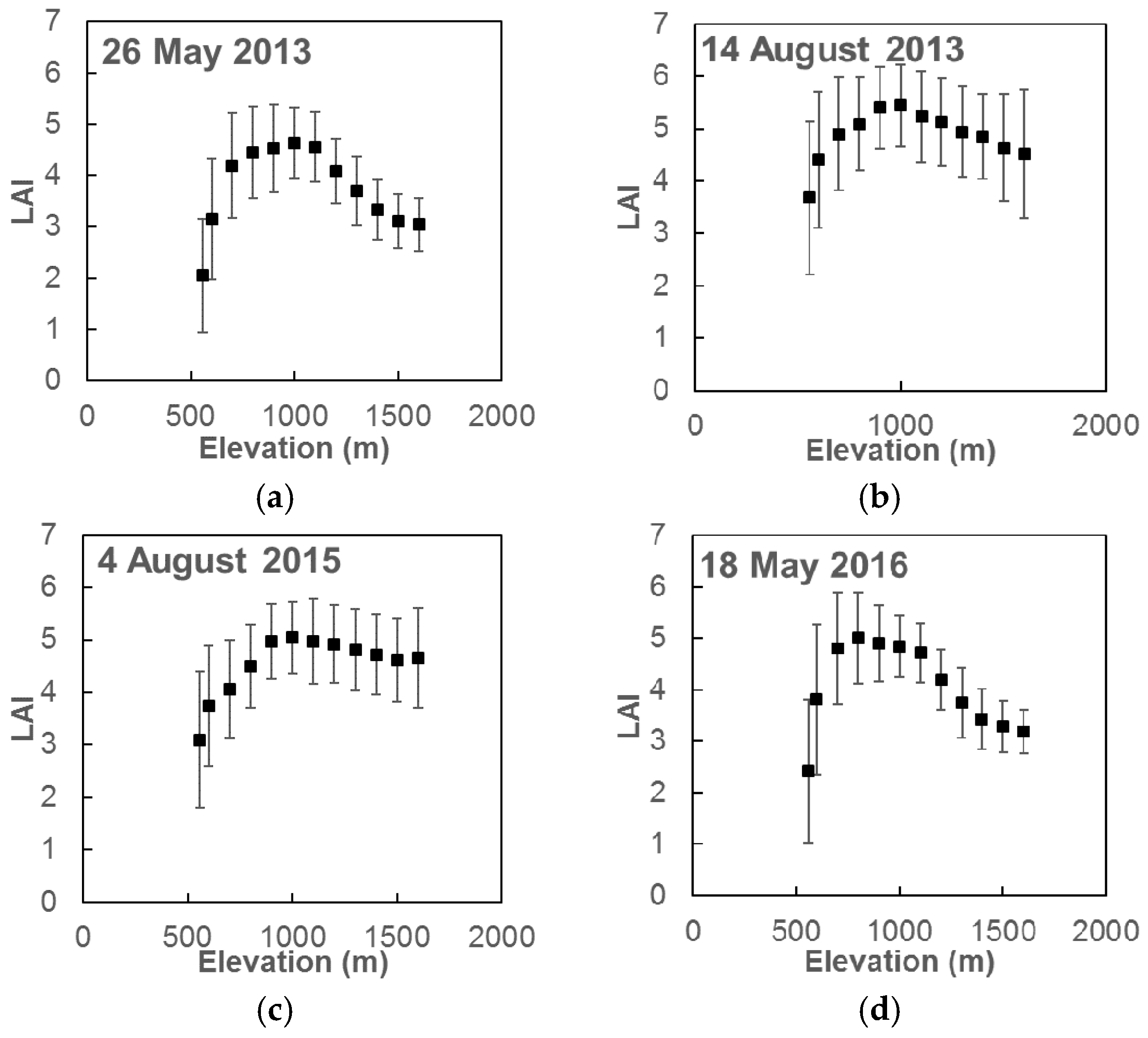
4.3. Spatial Leaf Area Index Variation

The resolution of 30 m allowed representation of the spatial variation of LAI in a mountainous landscape, a representation that could not be achieved by moderate (1000-m) resolution products such as MOD15A2 (Figure 6). In the study area, LAI was altered by anthropogenic disturbances at low elevations, where the city of Takayama (with a population of about 90,000 people) and agricultural facilities (mostly rice paddies) were located. With the decrease of anthropogenic disturbance concomitant with increasing altitude, LAI increased to a maximum at 900–1100 m a.s.l. We conclude that the 900–1100 m a.s.l. zone is favorable for DBF in the study area. Above this elevation range of maximum LAI, the LAI decreased primarily because of the decline of air temperature with altitude. Larger decreases in the spring LAI at elevations >1100 m a.s.l. were associated with the delay in leaf expansion timing, whereas the smaller decrease of the LAI in summer (August) was related to the shorter growing season (lower temperature) at high elevations. The described altitudinal gradient limits net primary productivity and therefore affects both the structure and functions of the ecosystem [14].
The summer maximum LAI in the DBF areas of the Daihachiga river basin, estimated by the simple model, was slightly higher in 2013 than in 2015. Because the study area was under the influence of the Asian Monsoon and because water was not a limiting factor [2,66], we hypothesize that temperature was among the factors that largely contributed to the interannual LAI variation. The summer mean air temperature at TKY was 17.6 °C in 2013 and 16.9 °C in 2015, whereas the in situ maximum LAI estimated by the PAR transmittance method equaled 5.9 ± 0.4 in 2013 and 5.2 ± 0.4 in 2015, respectively. The higher spring temperatures resulted in a higher spatial average of the spring LAI in 2016 compared to 2013. The difference of the LAI between the two study years was apparent at lower altitudes and declined with increases of ground elevation (Figure 8). The fact that the rate of LAI decreases at higher altitudes appeared identical in maps based on the two spring images confirmed the altitudinal gradient of the degree of leaf expansion. Although the study period (2013–2016) was insufficient for a thorough analysis of interannual LAI variation, the estimates based on the summer Landsat OLI imagery demonstrated an altitudinal gradient of forest foliage density. The LAI decreased from its maximum value at 1000–1100 m a.s.l. by 20–30% at 1500–1600 m a.s.l.

5. Conclusions

The dependence of LAI on temperature has been evidenced in numerous ecological studies with respect to spatial variations [1,7,23,40,67] and leaf seasonality [2,38]. This study demonstrated the importance of accurate, fine-resolution spatial LAI estimation for ecological studies in areas of complex topography and high vegetative heterogeneity. The simple model revealed an altitudinal gradient of the degree of leaf expansion and summer maximum foliage density in a mountain forest.
The pre-processing of Landsat OLI imagery was a critical component of this study because of the complex atmospheric and topographic conditions that affect LAI estimation by the remote sensing approach. The elevation-dependent DOS corrected for the vertically non-homogeneous atmospheric conditions, and the Minnaert correction reduced the shadows of mountain slopes. The used LAI estimation model benefitted from its simplicity and was adaptable for various forest ecosystems. The next step to validate the accuracy and improve the simple model would be creating a larger sample of study plots with a carefully designed sampling strategy. In addition, further applications of the simple model to moderate resolution satellite imagery (e.g., MODIS) and a comparison of the resultant LAI estimates with available LAI products of an equivalent spatial resolution would contribute to the improvement of existing LAI estimation algorithms.

Acknowledgments

We thank Kenji Kurumado, Yasumasa Hiomo, and Koji Suzuki of the Takayama field station of Gifu University for their continued support of this research. We also want to thank Toshiyuki Ohtsuka, Shinpei Yoshitake (Gifu University), Hiroshi Koizumi (Waseda University), and Shohei Murayama (National Institute of Advanced Industrial Science and Technology), who generously supplied necessary data, and Toshiharu Kojima (Gifu University) for technical advice concerning data analysis. We thank the Gifu Prefecture government for providing the aerial photography composite of the study area. Special thanks to Shin Nagai (Japan Agency for Marine-Earth Science and Technology) and Hirokazu Yamamoto (National Institute of Advanced Industrial Science and Technology) for valuable advice and suggestions for the research. This study was partly supported by “JSPS KAKENHI Grant Number JP26241005” to HM and by the Social Implementation Program on Climate Change Adaptation Technology (SI-CAT).

Author Contributions

Irina Melnikova performed the data analysis and wrote the paper. Hiroyuki Muraoka, Yoshio Awaya, Taku M. Saitoh, and Takahiro Sasai coordinated the research and contributed to supervision of the methods employed. All the authors worked on editing and revising the manuscript.

Conflicts of Interest

The authors declare no conflict of interest.

Appendix A

In situ LAI at TKY was estimated by two methods―litter-fall collection and gap-fraction, LAI at C18―by litter-fall collection, LAI at L50 and TKC―by allometry. At TKY, continuous in situ measurements at 5-min intervals of incoming PAR above the forest canopy (on the top of an eco-tower, 18 m above the ground) and in the understory (just above the understory vegetation, ca. 2 m above the ground) were used to estimate LAI in 2013 [2]. To eliminate the effects of weather, we only used PAR measurements made on cloudy days; cloudy days were determined using the method described by Saitoh et al. [32,55]. The seasonal LAI was estimated based on the PAR transmittance method [3,21]. In addition, LAI at the Takayama site was validated by litter-fall collection [4], using Equation (A1):
LAI = T o t a l   l e a f   d r y   m a s s L M A ,
where LMA is leaf mass per leaf area (g m−2) at the single-leaf level (we used the mean LMA of the dominant species at TKY, averaged based on the fraction of their basal areas to the total basal area, 69.26 g m−2 [4,36]). At C18, the summer LAI, which was considered to be the maximum LAI of all seasons, was calculated from the measurements of annual litter production [35] using Equation (A1) with the same LMA value, as at TKY. At L50 and TKC, LAI was estimated using Equation (A1), where total leaf dry mass was derived from allometric equations [68,69]. We used the inventory datasets (produced in 2006) and LMA equal to 77.3 g m−2 [57] for L50 and LMA equal to 343.78 ± 16.06 g m−2 (estimation from a sample of 15 shoots of Japanese cedar with lengths of approximately 1.5–15 cm) for TKC. Because L50 and TKC represent mature forests, we assumed the stem growth after the forest inventory to have a negligible effect on the LAI estimated by allometry. In addition, the extinction coefficient for ECF was estimated from allometry-based LAI estimates and PAR-measurements at TKC in 2006 by transforming Equation (7) to:
k = L A I 1 ln ( P A R t / P A R 0 ) .

Appendix B

Figure A1. Linear regressions of MIN DN on elevation for bands 2–4 of Landsat OLI sub-images dated 26 May 2013 (ac), 14 August 2013 (df), 4 August 2015 (gi), and 18 May 2016 (jl), respectively.
Remotesensing 10 00179 g0a1

References

  1. Bonan, G.B. Forests and climate change: forcings, feedbacks, and the climate benefits of forests. Science 2008, 320, 1444–1449. [Google Scholar] [CrossRef] [PubMed]
  2. Muraoka, H.; Saigusa, N.; Nasahara, K.N.; Noda, H.; Yoshino, J.; Saitoh, T.M.; Nagai, S.; Murayama, S.; Koizumi, H. Effects of seasonal and interannual variations in leaf photosynthesis and canopy leaf area index on gross primary production of a cool-temperate deciduous broadleaf forest in Takayama, Japan. J. Plant Res. 2010, 123, 563–576. [Google Scholar] [CrossRef] [PubMed]
  3. Muraoka, H.; Noda, H.M.; Nagai, S.; Motohka, T.; Saitoh, T.M.; Nasahara, K.N.; Saigusa, N. Spectral vegetation indices as the indicator of canopy photosynthetic productivity in a deciduous broadleaf forest. J. Plant Ecol. 2012, 6, 393–407. [Google Scholar] [CrossRef]
  4. Nasahara, K.N.; Muraoka, H.; Nagai, S.; Mikami, H. Vertical integration of leaf area index in a Japanese deciduous broad-leaved forest. Agric. For. Meteorol. 2008, 148, 1136–1146. [Google Scholar] [CrossRef] [Green Version]
  5. Eriksson, H.; Eklundh, L.; Hall, K.; Lindroth, A. Estimating LAI in deciduous forest stands. Agric. For. Meteorol. 2005, 129, 27–37. [Google Scholar] [CrossRef]
  6. Biudes, M.S.; Machado, N.G.; Danelichen, V.H.; Souza, M.C.; Vourlitis, G.L.; Nogueira, J.D.S. Ground and remote sensing-based measurements of leaf area index in a transitional forest and seasonal flooded forest in Brazil. Int. J. Biometeorol. 2014, 58, 1181–1193. [Google Scholar] [CrossRef] [PubMed]
  7. Sprintsin, M.; Karnieli, A.; Berliner, P.; Rotenberg, E.; Yakir, D.; Cohen, S. The effect of spatial resolution on the accuracy of leaf area index estimation for a forest planted in the desert transition zone. Remote Sens. Environ. 2007, 109, 416–428. [Google Scholar] [CrossRef]
  8. Watson, D. Comparative physiological studies on the growth of field crops: II. The effect of varying nutrient supply on net assimilation rate and leaf area. Ann. Bot. 1947, 11, 375–407. [Google Scholar] [CrossRef]
  9. Chen, J.M.; Black, T. Defining leaf area index for non-flat leaves. Plant Cell Environ. 1992, 15, 421–429. [Google Scholar] [CrossRef]
  10. Myneni, R.B.; Ramakrishna, R.; Nemani, R.; Running, S.W. Estimation of global leaf area index and absorbed PAR using radiative transfer models. IEEE Trans. Geosci. Remote Sens. 1997, 35, 1380–1393. [Google Scholar] [CrossRef]
  11. Olivas, P.C.; Oberbauer, S.F.; Clark, D.B.; Clark, D.A.; Ryan, M.G.; O’Brien, J.J.; Ordonez, H. Comparison of direct and indirect methods for assessing leaf area index across a tropical rain forest landscape. Agric. For. Meteorol. 2013, 177, 110–116. [Google Scholar] [CrossRef]
  12. White, J.D.; Running, S.W.; Nemani, R.; Keane, R.E.; Ryan, K.C. Measurement and remote sensing of LAI in Rocky Mountain montane ecosystems. Can. J. For. Res. 1997, 27, 1714–1727. [Google Scholar] [CrossRef]
  13. Manninen, T.; Korhonen, L.; Voipio, P.; Lahtinen, P.; Stenberg, P. Leaf Area Index (LAI) Estimation of Boreal Forest Using Wide Optics Airborne Winter Photos. Remote Sens. 2009, 1, 1380–1394. [Google Scholar] [CrossRef]
  14. Bolstad, P.V.; Vose, J.M.; McNulty, S.G. Forest productivity, leaf area, and terrain in southern Appalachian deciduous forests. For. Sci. 2001, 47, 419–427. [Google Scholar]
  15. Knyazikhin, Y.; Martonchik, J.; Diner, D.; Myneni, R.; Verstraete, M.; Pinty, B.; Gobron, N. Estimation of vegetation canopy leaf area index and fraction of absorbed photosynthetically active radiation from atmosphere-corrected MISR data. J. Geophys. Res. Atmos. 1998, 103, 32239–32256. [Google Scholar] [CrossRef]
  16. Zhu, Z.; Bi, J.; Pan, Y.; Ganguly, S.; Anav, A.; Xu, L.; Samanta, A.; Piao, S.; Nemani, R.R.; Myneni, R.B. Global data sets of vegetation leaf area index (LAI) 3g and Fraction of Photosynthetically Active Radiation (FPAR) 3g derived from Global Inventory Modeling and Mapping Studies (GIMMS) Normalized Difference Vegetation Index (NDVI3g) for the period 1981 to 2011. Remote Sens. 2013, 5, 927–948. [Google Scholar]
  17. Spanner, M.A.; Pierce, L.L.; Peterson, D.L.; Running, S.W. Remote sensing of temperate coniferous forest leaf area index. The influence of canopy closure, understory vegetation and background reflectance. Int. J. Remote Sens. 1990, 11, 95–111. [Google Scholar] [CrossRef]
  18. Peterson, D.L.; Spanner, M.A.; Running, S.W.; Teuber, K.B. Relationship of thematic mapper simulator data to leaf area index of temperate coniferous forests. Remote Sens. Environ. 1987, 22, 323–341. [Google Scholar] [CrossRef]
  19. Nagai, S.; Inoue, T.; Ohtsuka, T.; Kobayashi, H.; Kurumado, K.; Muraoka, H.; Nasahara, K.N. Relationship between spatio-temporal characteristics of leaf-fall phenology and seasonal variations in near surface-and satellite-observed vegetation indices in a cool-temperate deciduous broad-leaved forest in Japan. Int. J. Remote Sens. 2014, 35, 3520–3536. [Google Scholar] [CrossRef]
  20. Jonckheere, I.; Fleck, S.; Nackaerts, K.; Muys, B.; Coppin, P.; Weiss, M.; Baret, F. Review of methods for in situ leaf area index determination: Part I. Theories, sensors and hemispherical photography. Agric. For. Meteorol. 2004, 121, 19–35. [Google Scholar] [CrossRef]
  21. Monsi, M.; Saeki, T. On the factor light in plant communities and its importance for matter production. Ann. Bot. 2005, 95, 549–567. [Google Scholar] [CrossRef] [PubMed]
  22. Liang, S.; Li, X.; Wang, J. Advanced Remote Sensing: Terrestrial Information Extraction and Applications, 1st ed.; Academic Press, Elsevier: Oxford, UK, 2012; pp. 347–380. [Google Scholar]
  23. Propastin, P.; Kappas, M. Retrieval of coarse-resolution leaf area index over the Republic of Kazakhstan using NOAA AVHRR satellite data and ground measurements. Remote Sens. 2012, 4, 220–246. [Google Scholar] [CrossRef]
  24. Gray, J.; Song, C. Mapping leaf area index using spatial, spectral, and temporal information from multiple sensors. Remote Sens. Environ. 2012, 119, 173–183. [Google Scholar] [CrossRef]
  25. Baret, F.; Guyot, G. Potentials and limits of vegetation indices for LAI and APAR assessment. Remote Sens. Environ. 1991, 35, 161–173. [Google Scholar] [CrossRef]
  26. Susaki, J.; Hara, K.; JongGeol, P.; Yasuda, Y.; Kajiwara, K.; Honda, Y. Validation of temporal BRDFs of paddy fields estimated from MODIS reflectance data. IEEE Trans. Geosci. Remote Sens. 2004, 42, 1262–1270. [Google Scholar] [CrossRef]
  27. Sasai, T.; Saigusa, N.; Nasahara, K.N.; Ito, A.; Hashimoto, H.; Nemani, R.; Hirata, R.; Ichii, K.; Takagi, K.; Saitoh, T.M. Satellite-driven estimation of terrestrial carbon flux over Far East Asia with 1-km grid resolution. Remote Sens. Environ. 2011, 115, 1758–1771. [Google Scholar] [CrossRef]
  28. Roy, D.P.; Wulder, M.A.; Loveland, T.R.; C.E, W.; Allen, R.G.; Anderson, M.C.; Helder, D.; Irons, J.R.; Johnson, D.M.; Kennedy, R.; et al. Landsat-8: Science and product vision for terrestrial global change research. Remote Sens. Environ. 2014, 145, 154–172. [Google Scholar] [CrossRef]
  29. Ke, Y.; Im, J.; Lee, J.; Gong, H.; Ryu, Y. Characteristics of Landsat 8 OLI-derived NDVI by comparison with multiple satellite sensors and in-situ observations. Remote Sens. Environ. 2015, 164, 298–313. [Google Scholar] [CrossRef]
  30. Awaya, Y. Forest type classification over Gujo city using NDVI based on phenology (in Japanese). In Proceedings of the 61st Autumn Conference of the Remote Sensing Society of Japan, Tokyo, Japan, 1–2 November 2016; pp. 251–252. [Google Scholar]
  31. Awaya, Y.; Takahashi, T. Evaluating the Differences in Modeling Biophysical Attributes between Deciduous Broadleaved and Evergreen Conifer Forests Using Low-Density Small-Footprint LiDAR Data. Remote Sens. 2017, 9, 572. [Google Scholar] [CrossRef]
  32. Saitoh, T.M.; Tamagawa, I.; Muraoka, H.; Lee, N.-Y.M.; Yashiro, Y.; Koizumi, H. Carbon dioxide exchange in a cool-temperate evergreen coniferous forest over complex topography in Japan during two years with contrasting climates. J. Plant Res. 2010, 123, 473–483. [Google Scholar] [CrossRef] [PubMed]
  33. Fukuda, N.; Awaya, Y.; Kojima, T. Classification of forest vegetation types using LiDAR data and Quickbird images—Case study of the Daihachiga river basin in Takayama. J. Jpn. Agric. Syst. Soc. 2012, 28, 115–122. [Google Scholar]
  34. SATECO. Gifu University 21st Century COE Program “Satellite Ecology”. Available online: http://www.green.gifu-u.ac.jp/sateco/eng/index.html (accessed on 17 January 2018).
  35. Ohtsuka, T.; Shizu, Y.; Nishiwaki, A.; Yashiro, Y.; Koizumi, H. Carbon cycling and net ecosystem production at an early stage of secondary succession in an abandoned coppice forest. J. Plant Res. 2010, 123, 393–401. [Google Scholar] [CrossRef] [PubMed]
  36. Ohtsuka, T.; Akiyama, T.; Hashimoto, Y.; Inatomi, M.; Sakai, T.; Jia, S.; Mo, W.; Tsuda, S.; Koizumi, H. Biometric based estimates of net primary production (NPP) in a cool-temperate deciduous forest stand beneath a flux tower. Agric. For. Meteorol. 2005, 134, 27–38. [Google Scholar] [CrossRef]
  37. Inoue, T.; Nagai, S.; Inoue, S.; Ozaki, M.; Sakai, S.; Muraoka, H.; Koizumi, H. Seasonal variability of soil respiration in multiple ecosystems under the same physical–geographical environmental conditions in central Japan. For. Sci. Technol. 2012, 8, 52–60. [Google Scholar] [CrossRef]
  38. Noda, H.M.; Muraoka, H.; Nasahara, K.N.; Saigusa, N.; Murayama, S.; Koizumi, H. Phenology of leaf morphological, photosynthetic, and nitrogen use characteristics of canopy trees in a cool-temperate deciduous broadleaf forest at Takayama, central Japan. Ecol. Res. 2015, 30, 247–266. [Google Scholar] [CrossRef]
  39. Saitoh, T.M.; Nagai, S.; Yoshino, J.; Kondo, H.; Tamagawa, I.; Muraoka, H. Effects of canopy phenology on deciduous overstory and evergreen understory carbon budgets in a cool-temperate forest ecosystem under ongoing climate change. Ecol. Res. 2015, 30, 267–277. [Google Scholar] [CrossRef]
  40. Kira, T. Forest ecosystems of east and southeast Asia in a global perspective. Ecol. Res. 1991, 6, 185–200. [Google Scholar] [CrossRef]
  41. Chavez, P.S. An improved dark-object subtraction technique for atmospheric scattering correction of multispectral data. Remote Sens. Environ. 1988, 24, 459–479. [Google Scholar] [CrossRef]
  42. USGS. Using the USGS Landsat 8 Product. Available online: https://landsat.usgs.gov/using-usgs-landsat-8-product (accessed on 17 January 2018).
  43. Liang, S.; Fang, H.; Chen, M. Atmospheric Correction of Landsat ETM+ Land Surface Imagery. Part I: Methods. IEEE Trans. Geosci. Remote Sens. 2001, 39, 2490–2498. [Google Scholar] [CrossRef]
  44. Williams, D.L. A comparison of spectral reflectance properties at the needle, branch, and canopy level for selected conifer species. Remote Sens. Environ. 1991, 35, 79–93. [Google Scholar] [CrossRef]
  45. Kaufman, Y.J. The atmospheric effect on remote sensing and its correction. In Theory and Applications of Optical Remote Sensing; Asrar, G., Ed.; Wiley: New York, NY, USA, 1989; pp. 336–428. [Google Scholar]
  46. Ge, H.; Lu, D.; He, S.; Xu, A.; Zhou, G.; Du, H. Pixel-based Minnaert correction method for reducing topographic effects on a Landsat 7 ETM+ image. Photogramm. Eng. Remote Sens. 2008, 74, 1343–1350. [Google Scholar] [CrossRef]
  47. Smith, J.; Lin, T.L.; Ranson, K. The Lambertian assumption and Landsat data. Photogramm. Eng. Remote Sens. 1980, 46, 1183–1189. [Google Scholar]
  48. Tokola, T.; Sarkeala, J.; Van der Linden, M. Use of topographic correction in Landsat TM-based forest interpretation in Nepal. Int. J. Remote Sens. 2001, 22, 551–563. [Google Scholar] [CrossRef]
  49. Awaya, T.; Kodani, E.; Iehara, T.; Hosoda, K.; Takahashi, T.; Sakai, T. Mapping leaf area index over Japanese Archipelago—Comparison of the results by plot data and MODIS data. In Proceedings of the 16th Seiken forum on earth environmental monitoring, University of Tokyo, Tokyo, Japan, 26–27 March 2007; pp. 88–91. (In Japanese). [Google Scholar]
  50. Chen, J.M.; Rich, P.M.; Gower, S.T.; Norman, J.M.; Plummer, S. Leaf area index of boreal forests: Theory, techniques, and measurements. J. Geophys. Res. Atmos. 1997, 102, 29429–29443. [Google Scholar] [CrossRef]
  51. Ross, J.; Sulev, M. Sources of errors in measurements of PAR. Agric. For. Meteorol. 2000, 100, 103–125. [Google Scholar] [CrossRef]
  52. Ridao, E.; Conde, J.R.; Mínguez, M.I. Estimating ƒAPAR from nine vegetation indices for irrigated and nonirrigated faba bean and semileafless pea canopies. Remote Sens. Environ. 1998, 66, 87–100. [Google Scholar] [CrossRef]
  53. Inoue, Y.; Olioso, A. Methods of Estimating Plant Productivity and CO 2 Flux in Agro-Ecosystems–Liking Measurements, Process Models, and Remotely Sensed Information. Elsevier Oceanogr. Ser. 2007, 73, 295–502. [Google Scholar]
  54. Jenkins, J.; Richardson, A.D.; Braswell, B.; Ollinger, S.V.; Hollinger, D.Y.; Smith, M.-L. Refining light-use efficiency calculations for a deciduous forest canopy using simultaneous tower-based carbon flux and radiometric measurements. Agric. For. Meteorol. 2007, 143, 64–79. [Google Scholar] [CrossRef]
  55. Saitoh, T.M.; Nagai, S.; Noda, H.M.; Muraoka, H.; Nasahara, K.N. Examination of the extinction coefficient in the Beer–Lambert law for an accurate estimation of the forest canopy leaf area index. For. Sci. Technol. 2012, 8, 67–76. [Google Scholar] [CrossRef]
  56. Hirata, R.; Hirano, T.; Saigusa, N.; Fujinuma, Y.; Inukai, K.; Kitamori, Y.; Takahashi, Y.; Yamamoto, S. Seasonal and interannual variations in carbon dioxide exchange of a temperate larch forest. Agric. For. Meteorol. 2007, 147, 110–124. [Google Scholar] [CrossRef]
  57. Koike, T.; Mao, Q.; Inada, N.; Kawaguchi, K.; Hoshika, Y.; Kita, K.; Watanabe, M. Growth and photosynthetic responses of cuttings of a hybrid larch (Larix gmelinii var. japonica x L. kaempferi) to elevated ozone and/or carbon dioxide. Asian J. Atmos. Environ. 2012, 6, 104–110. [Google Scholar] [CrossRef]
  58. Teillet, P.; Fedosejevs, G. On the dark target approach to atmospheric correction of remotely sensed data. Can. J. Remote Sens. 1995, 21, 374–387. [Google Scholar] [CrossRef]
  59. Kaufman, Y.J.; Sendra, C. Algorithm for automatic atmospheric corrections to visible and near-IR satellite imagery. Int. J. Remote Sens. 1988, 9, 1357–1381. [Google Scholar] [CrossRef]
  60. Chen, J.M.; Cihlar, J. Retrieving leaf area index of boreal conifer forests using Landsat TM images. Remote Sens. Environ. 1996, 55, 153–162. [Google Scholar] [CrossRef]
  61. Staelens, J.; Nachtergale, L.; Luyssaert, S.; Lust, N. A model of wind-influenced leaf litterfall in a mixed hardwood forest. Can. J. For. Res. 2003, 33, 201–209. [Google Scholar] [CrossRef]
  62. Smith, F.W.; Sampson, D.A.; Long, J.N. Notes: Comparison of leaf area index estimates from tree allometrics and measured light interception. For. Sci. 1991, 37, 1682–1688. [Google Scholar]
  63. Baldocchi, D.D.; Matt, D.R.; Hutchison, B.A.; McMillen, R.T. Solar radiation within an oak—Hickory forest: An evaluation of the extinction coefficients for several radiation components during fully-leafed and leafless periods. Agric. For. Meteorol. 1984, 32, 307–322. [Google Scholar] [CrossRef]
  64. Lee, B.; Kwon, H.; Miyata, A.; Lindner, S.; Tenhunen, J. Evaluation of a Phenology-Dependent Response Method for Estimating Leaf Area Index of Rice Across Climate Gradients. Remote Sens. 2017, 9, 20. [Google Scholar] [CrossRef]
  65. Li, C.; Song, J.; Wang, J. Modifying Geometric-Optical Bidirectional Reflectance Model for Direct Inversion of Forest Canopy Leaf Area Index. Remote Sens. 2015, 7, 11083–11104. [Google Scholar] [CrossRef]
  66. Setoyama, Y.; Sasai, T. Analyzing decadal net ecosystem production control factors and the effects of recent climate events in Japan. J. Geophys. Res. Biogeosci. 2013, 118, 337–351. [Google Scholar] [CrossRef]
  67. Parton, W.; Scurlock, J.; Ojima, D.; Gilmanov, T.; Scholes, R.; Schimel, D.; Kirchner, T.; Menaut, J.C.; Seastedt, T.; Garcia Moya, E. Observations and modeling of biomass and soil organic matter dynamics for the grassland biome worldwide. Glob. Biogeochem. Cycles 1993, 7, 785–809. [Google Scholar] [CrossRef]
  68. Watanabe, H.; Mogi, Y. Soil carbon stocks in mature Sugi and Hinoki stands. Bull. Gifu Prefect. Res. Inst. For. 2005, 34, 11–18. (In Japanese) [Google Scholar]
  69. Schulze, E.-D.; Schulze, W.; Koch, H.; Arneth, A.; Bauer, G.; Kelliher, F.; Hollinger, D.; Vygodskaya, N.; Kusnetsova, W.; Sogatchev, A. Aboveground biomass and nitrogen nutrition in a chronosequence of pristine Dahurian Larix stands in eastern Siberia. Can. J. For. Res. 1995, 25, 943–960. [Google Scholar] [CrossRef]
Figure 1. Forest types in the Daihachiga river basin by Fukuda et al., 2012 [33] with a 2-m spatial resolution, and the location of the four study plots.
Remotesensing 10 00179 g001
Figure 2. LAI of forest canopy as a function of cumulative effective temperature >2 °C (CET2) during the leaf expansion period of 2013 at TKY. The line represents the model, and squares are estimated LAI values.
Remotesensing 10 00179 g002
Figure 3. Original Landsat OLI sub-images dated 26 May 2013 (a); 14 August 2013 (b); 4 August 2015 (c); and 18 May 2016 (d). Yellow polygons denote the Daihachiga river basin. OLI bands 6, 5, and 4 are shown in red, green, and blue, respectively.
Remotesensing 10 00179 g003
Figure 4. Reflectance of ECF pixels at two different altitudes (601 m a.s.l. and 1289 m a.s.l.) before atmospheric correction (a,d,g,j), after elevation-dependent DOS (b,e,h,k), and after the application of additional offset (c,f,i,l) for Landsat OLI sub-images dated 26 May 2013, 14 August 2013, 4 August 2015, and 18 May 2016, respectively.
Remotesensing 10 00179 g004
Figure 5. Mountainous area before (a,b) and after (c,d) topographic correction for sub-images dated 26 May 2013 (a,c) and 14 August 2013 (b,d); OLI bands 4, 3, and 2 correspond to red, green, and blue colors, respectively.
Remotesensing 10 00179 g005
Figure 6. LAI estimations based on Landsat OLI sub-images dated 26 May 2013, 14 August 2013, 4 August 2015, and 18 May 2016, and the LAI map from the MOD15A2 dated 25 May 2013 over the Daihachiga river basin. The red color (LAI = 0) outlines the urban areas, grasslands, water objects, rice paddies, crops, and bare lands.
Remotesensing 10 00179 g006
Figure 7. Scatterplot between Landsat OLI imagery–based LAI estimations and ground truth LAI for the four study plots dated 26 May 2013 (a) and 14 August 2013 (b). Error bars represent standard errors.
Remotesensing 10 00179 g007
Figure 8. Spatial average LAI of DBF area for each 100-m altitudinal zone based on Landsat OLI sub-images dated 26 May 2013 (a); 14 August 2013 (b); 4 August 2015 (c); and 18 May 2016 (d) over the Daihachiga river basin. Error bars represent standard deviations.
Remotesensing 10 00179 g008
Table 1. Information about the four study plots.
Plot CodeLocationAltitude (m a.s.l.)Forest TypeDominant SpeciesForest Age (years)Plot Size (m2)Annual Mean Air Temperature (°C) Annual Precipitation (mm)References
TKY36°08′46″N, 137°25′23″E1420DBFQuercus crispula, Betula ermanii, Betula platyphylla var. japonica50–60100 × 1006.62400[36]
TKC36°08′24″N, 137°22′15″E800ECFCryptomeria japonica40–5030 × 5011.21723[3,32]
C1836°08′22″N, 137°23′17″E1160DBFBetula platyphylla var. japonica, Castanea crenata, Quercus crispula3020 × 307.2NA*[35]
L5036°08′04″N, 137°25′41″E1330DCFLarix kaempferi50–6030 × 307.22075[37]
* NA: Not available.
Table 2. Information of the Landsat OLI imagery used in this study.
Image DateSun Elevation Angle (°)Cloud Coverage (%)
26 May 201367.366.49
14 August 201361.071.82
4 August 201562.689.90
18 May 201665.870.35
Table 3. Linear regressions of MIN DN on elevation for three visible bands of four Landsat OLI sub-images.
Image DateOLI BandRegression *R2
26 May 2013Bluey = −0.61x + 9385.340.91
Greeny = −0.56x + 8577.350.88
Redy = −0.48x + 7400.110.97
14 August 2013Bluey = −0.55x + 8811.870.97
Greeny = −0.48x + 7605.490.98
Redy = −0.39x + 6674.140.82
4 August 2015Bluey = −0.50x + 8969.580.98
Greeny = −0.65x + 8011.620.96
Redy = −0.36x + 6787.980.94
18 May 2016Bluey = −0.42x + 8431.080.87
Greeny = −0.49x + 7456.110.97
Redy = −0.34x + 6572.350.84
* x is ground elevation (m a.s.l.); y is MIN DN.
Table 4. RF offset, determined by a comparison of visible spectral reflectance of ECF with Norway spruce measured by the airborne Spectrometer.
Image DateImage Reflectance of Dark ECF PixelsOffset RF
Blue (%)Green (%)Red (%)Blue (%)Green (%)Red (%)
26 May 20130.6 ± 0.2 *1.1 ± 0.10.9 ± 0.11.32.81.0
14 August 20130.6 ± 0.01.0 ± 0.10.8 ± 0.11.32.91.1
4 August 20150.5 ± 0.10.6 ± 0.10.4 ± 0.21.42.31.5
18 May 20161.4 ± 0.11.3 ± 0.11.4 ± 0.10.52.60.5
Norway spruce [44]1.9 ± 0.23.9 ± 0.41.9 ± 0.2---
* Standard deviation of adjacent pixels.
Table 5. Estimation of in situ LAI at the four study plots.
Plot CodeEstimation MethodMaximum LAISpring LAI *
TKYPAR transmittance5.9 ± 0.41.7
TKYLitter-fall collection5.0 ± 0.5-
TKCAllometry7.37.3
C18Litter-fall collection5.25.1
L50Allometry7.67.0
* Spring LAI was projected using phenological model at three deciduous forest study plots for 26 May 2013.

