Wind Direction Signatures in GNSS-R Observables from Space

 , , , , and
Abstract
:
1. Introduction
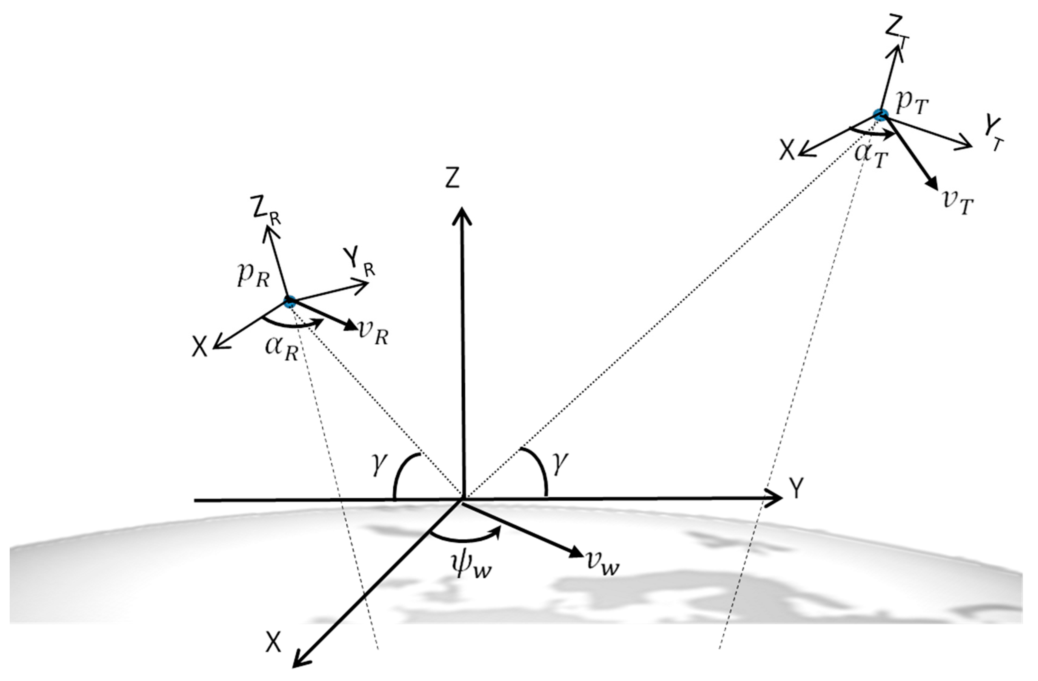
2. Methodology
2.1. Theoretical Background of Wind Speed Retrieval from the DDM
2.2. Simulation Studies
3. Results and Discussion
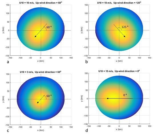
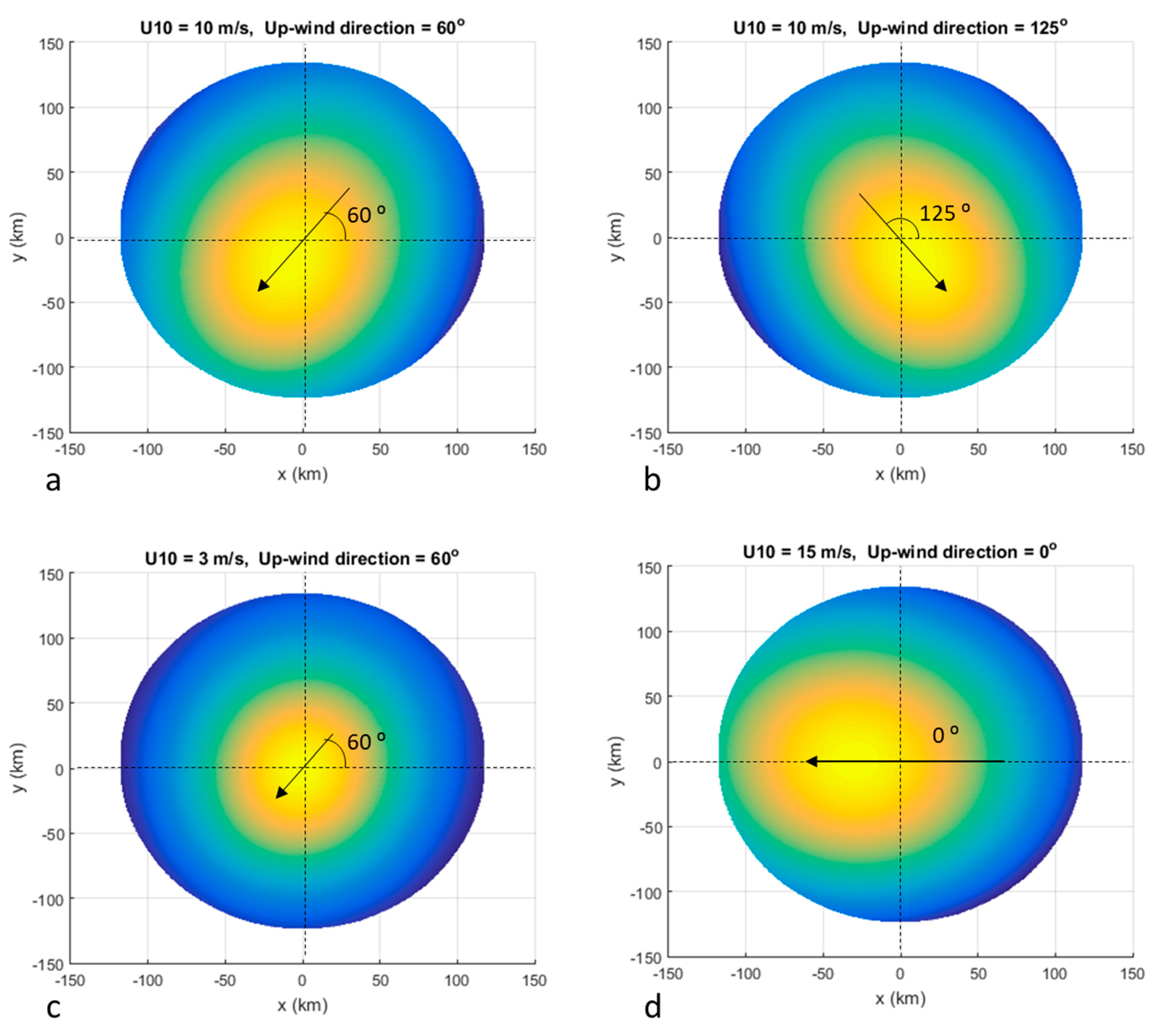
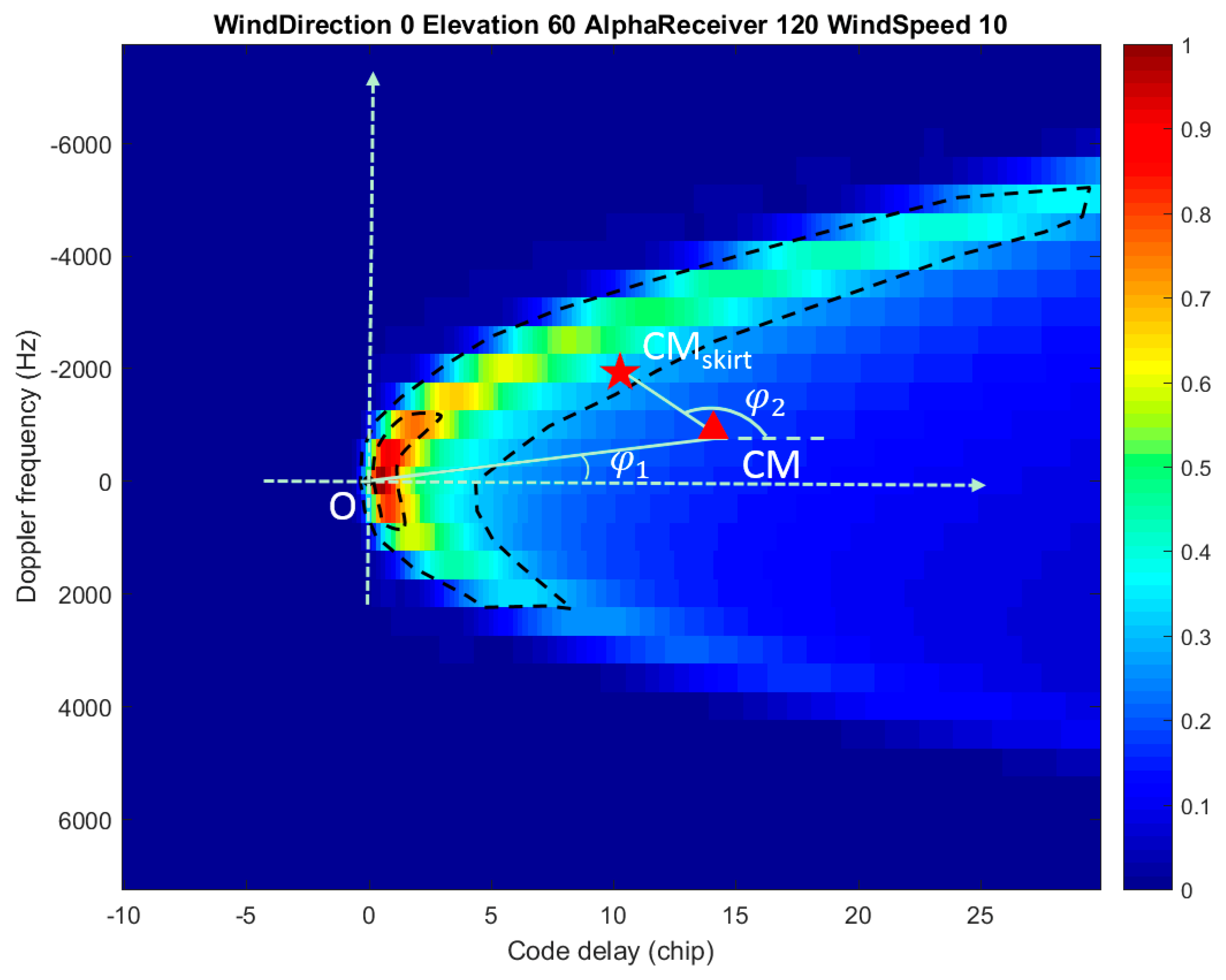
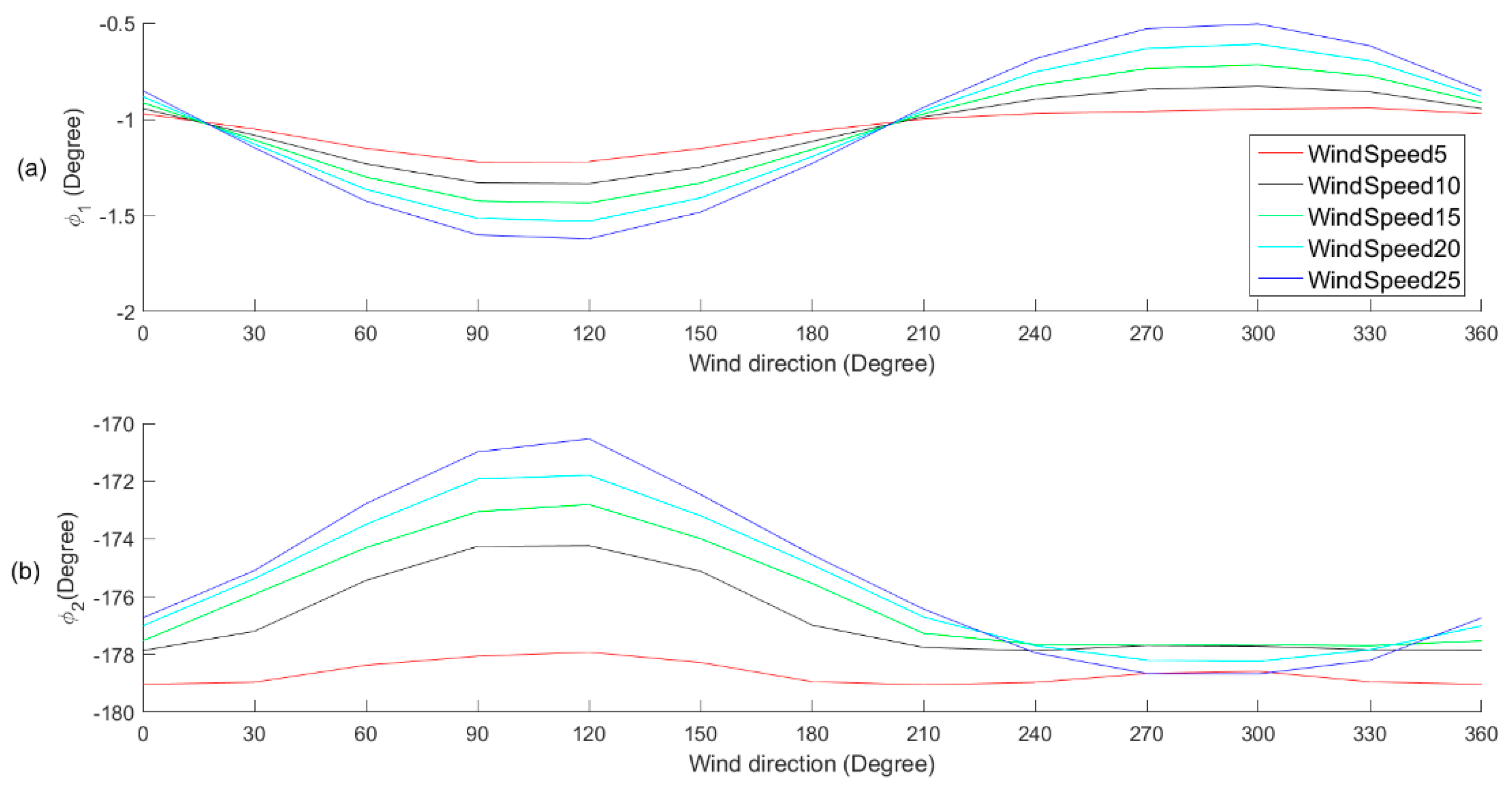
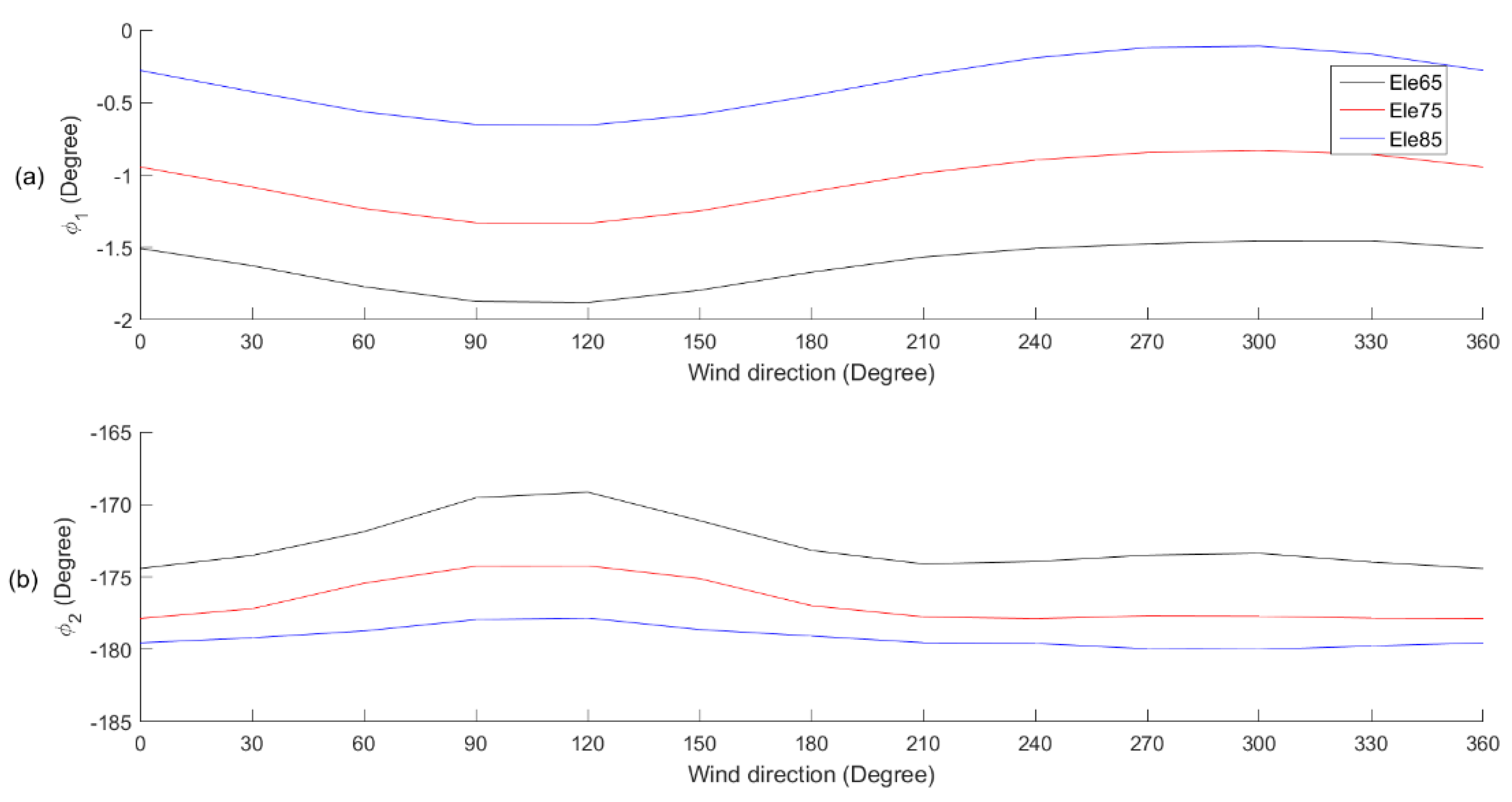
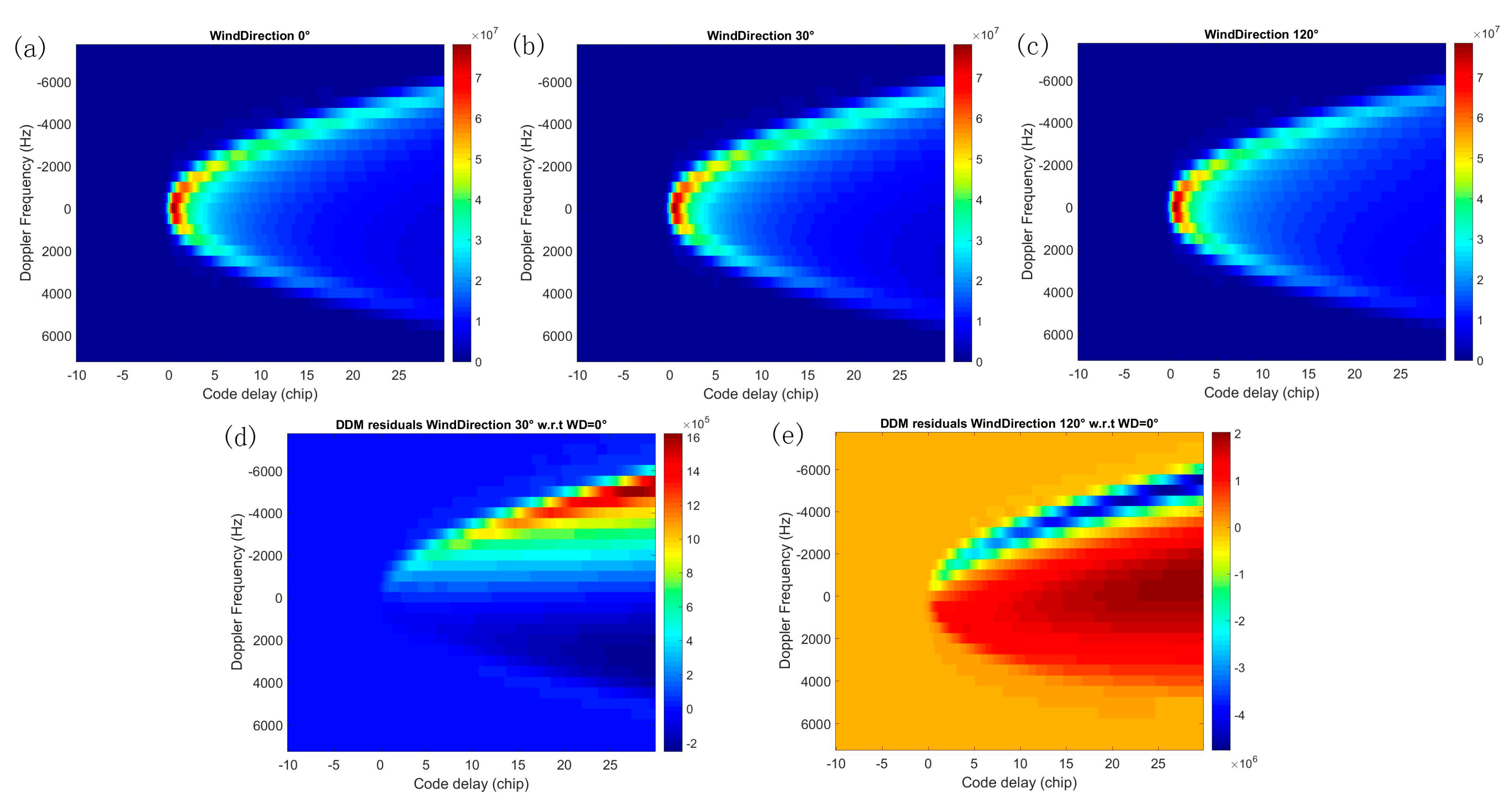
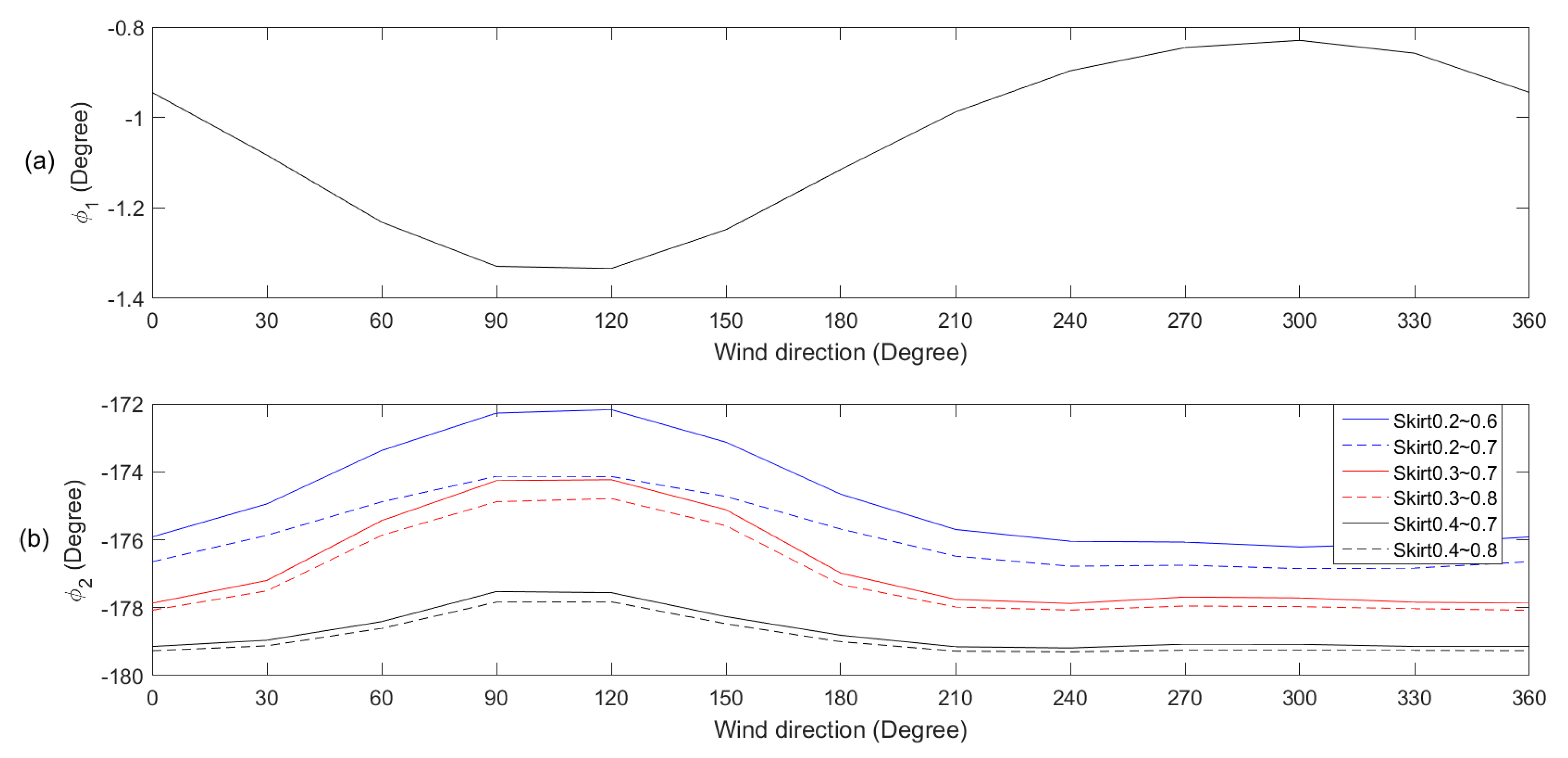
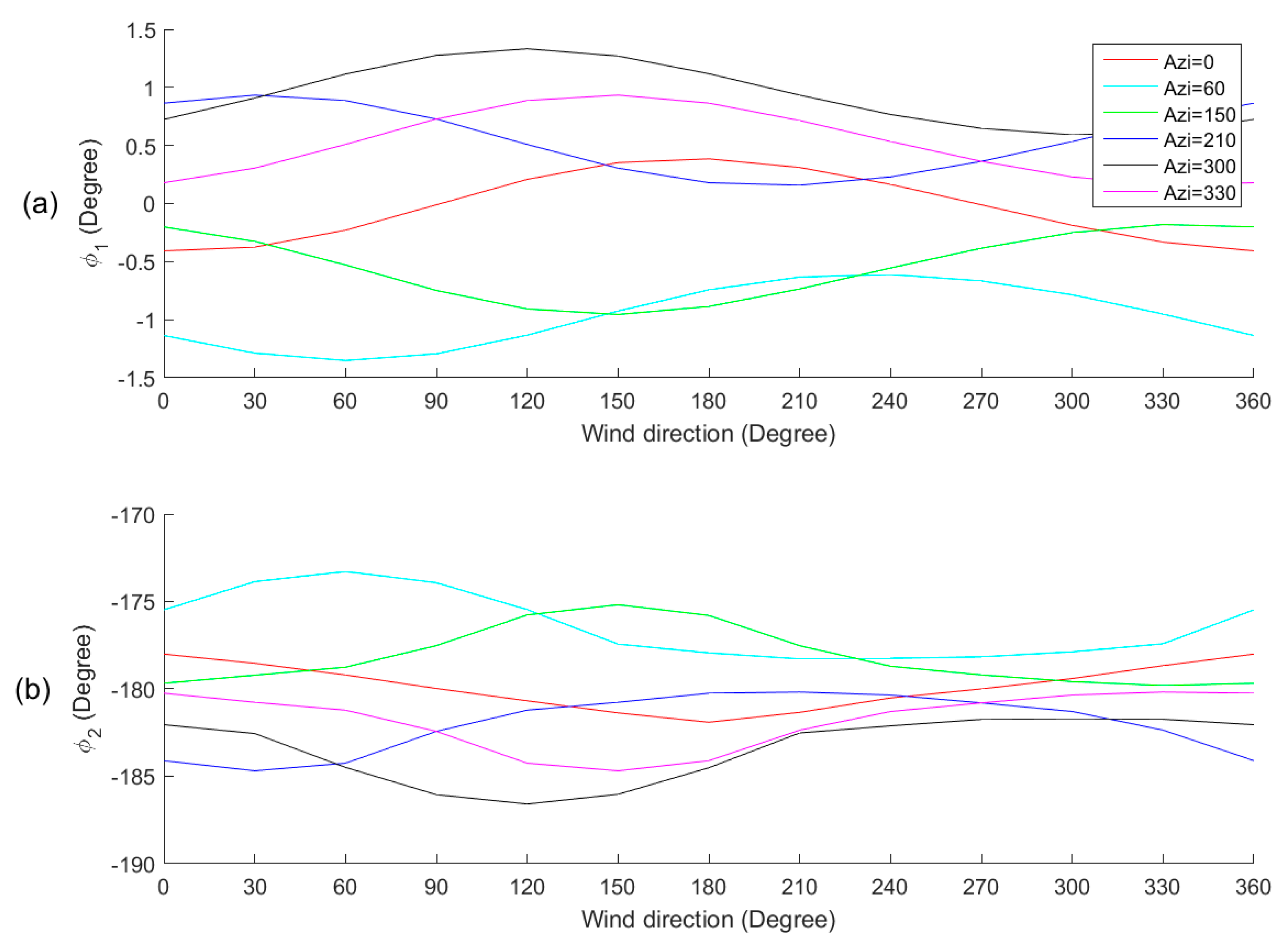
3.1. DDM Variations Caused by Wind Direction Changes
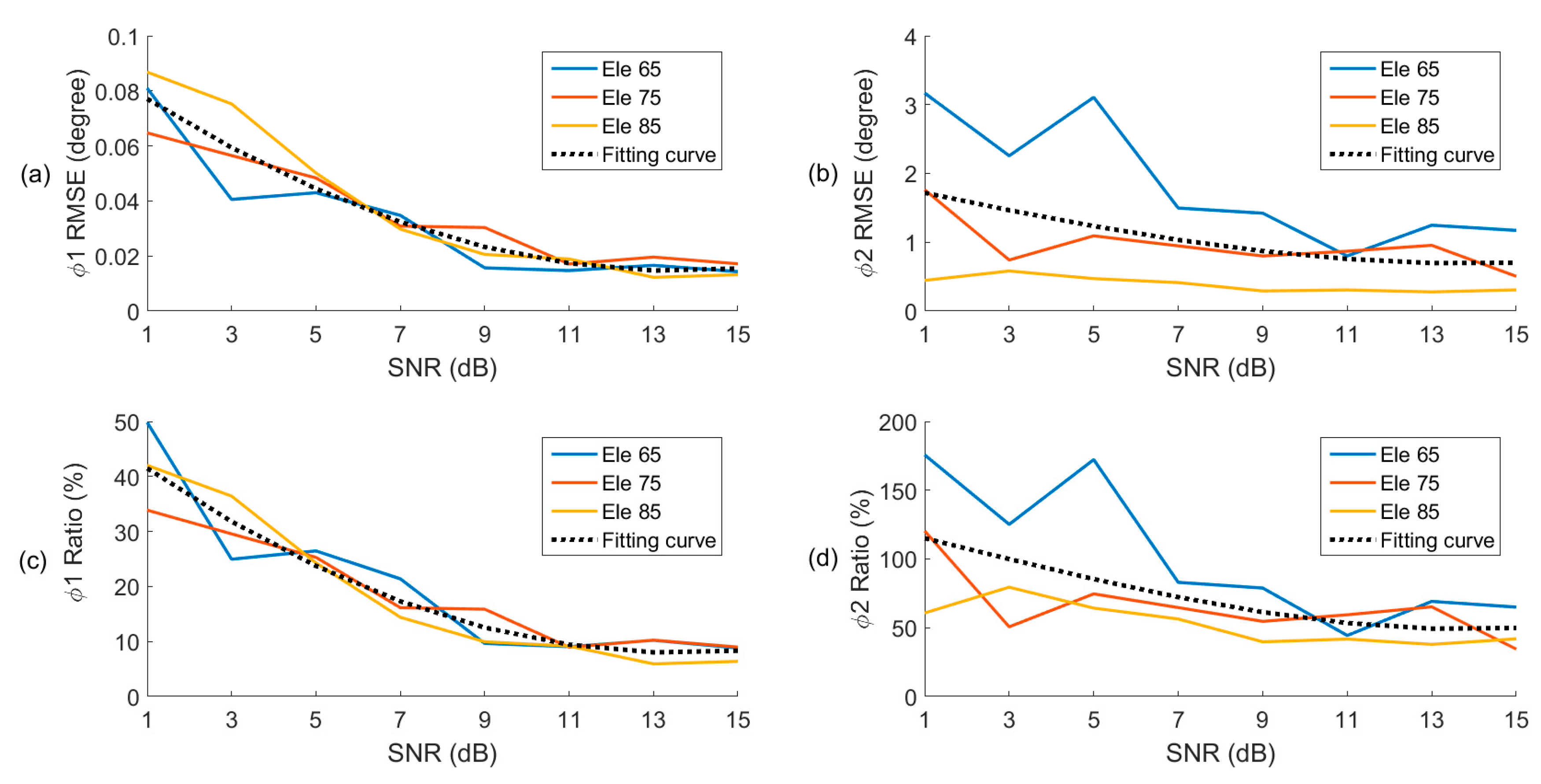
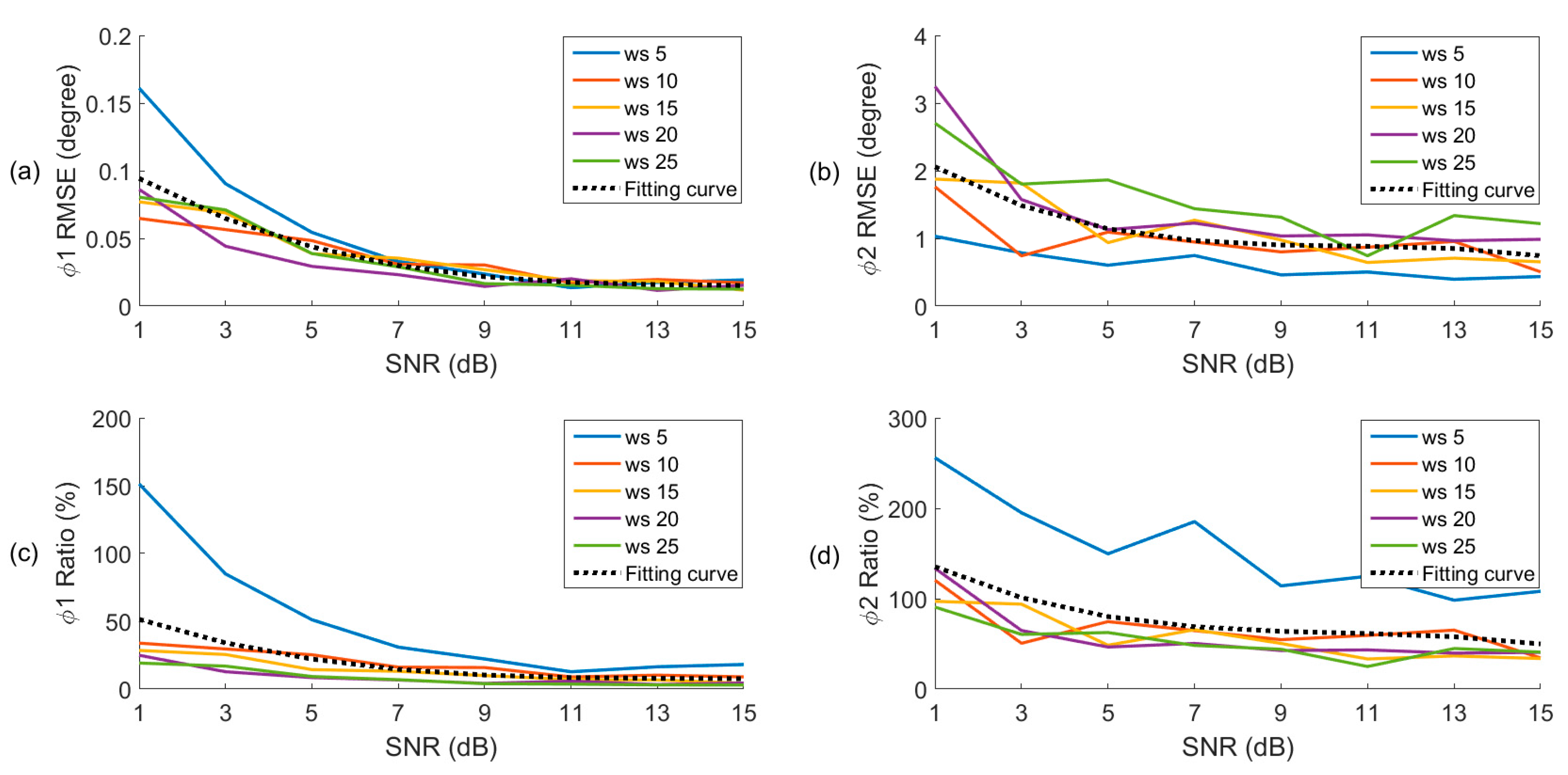
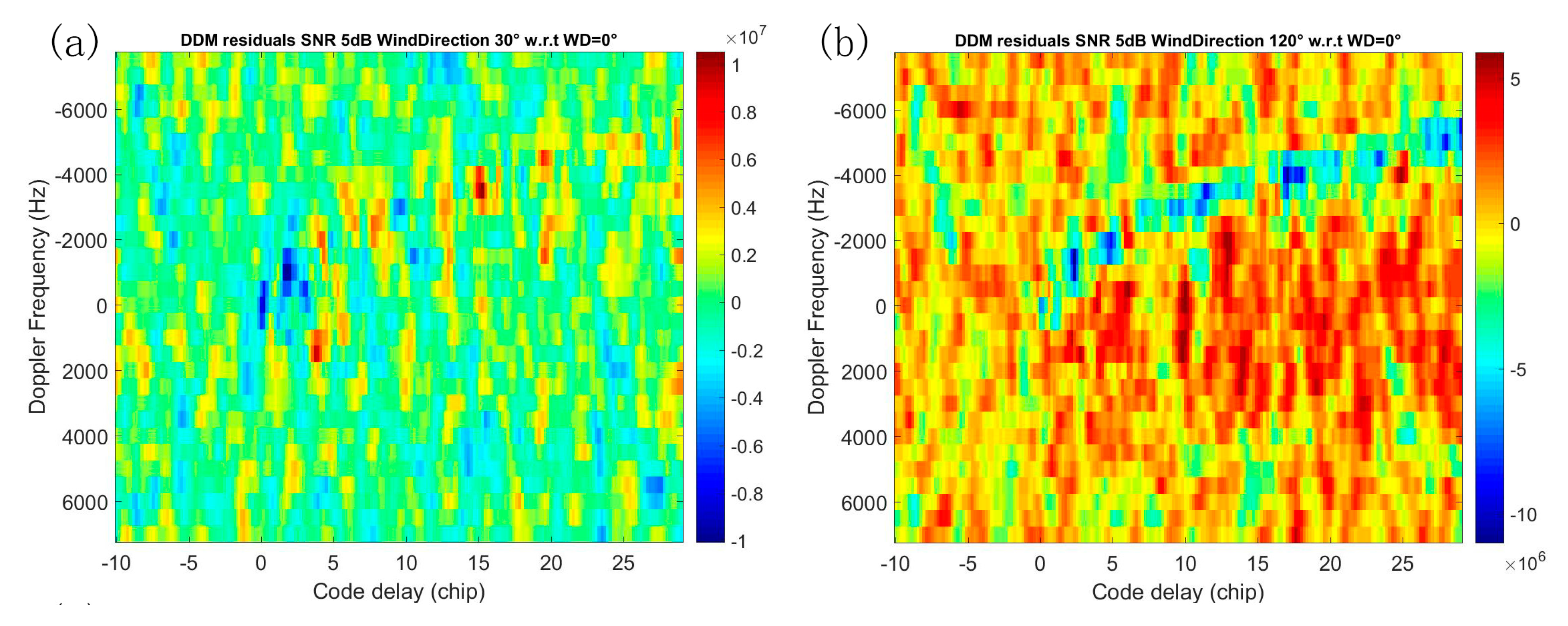
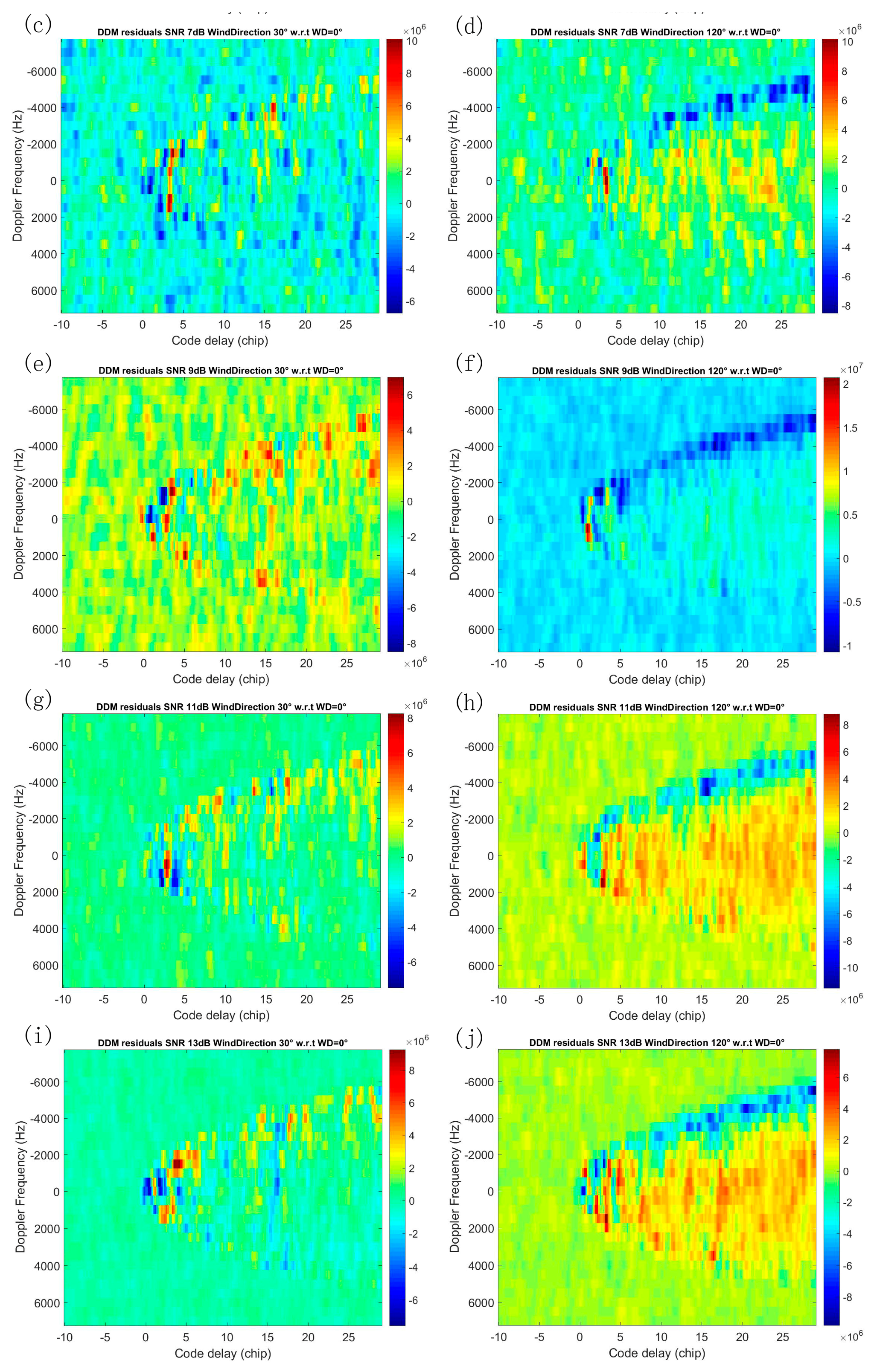
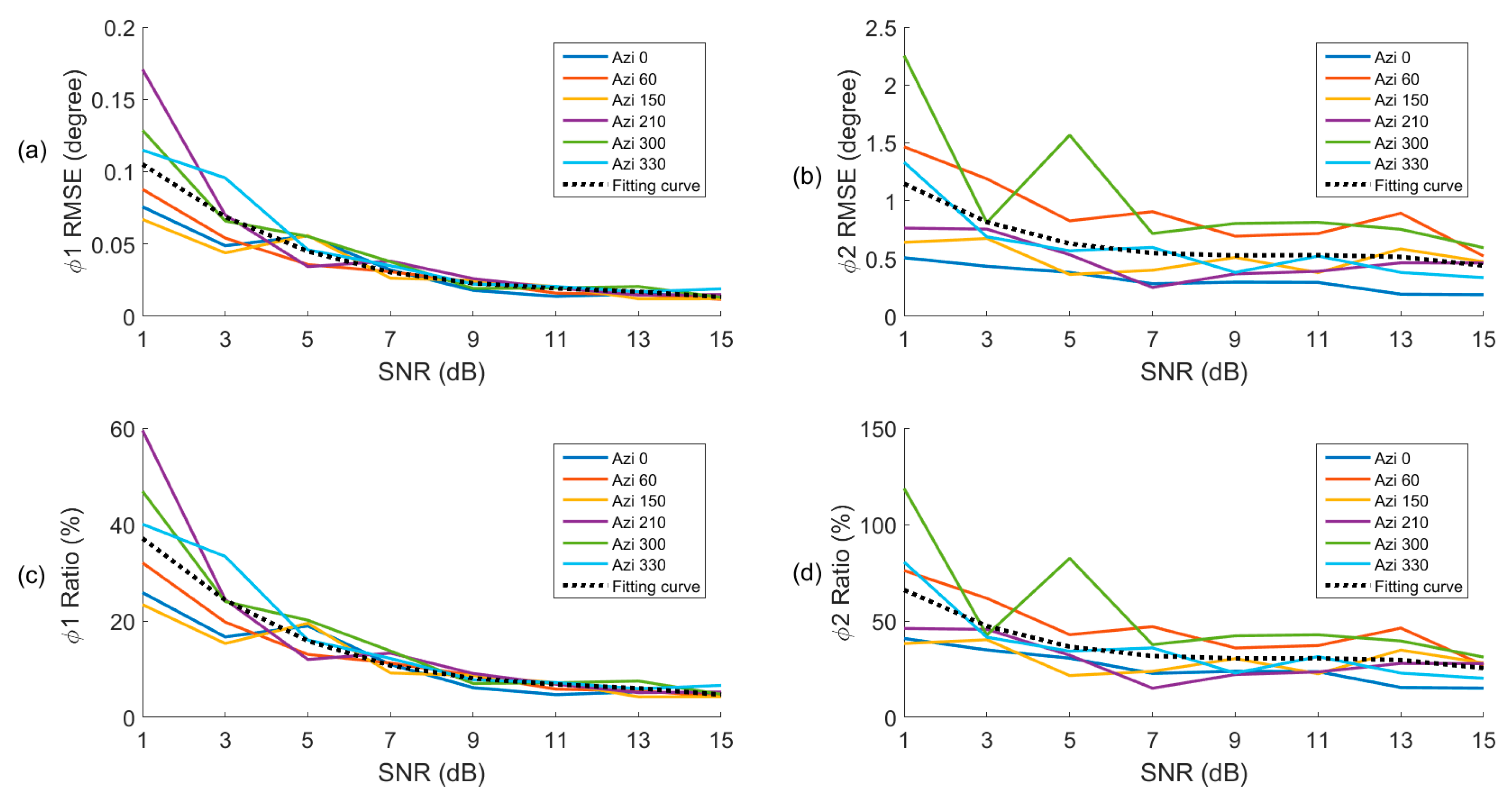
3.2. Effect of Noise
4. Conclusions
Acknowledgments
Author Contributions
Conflicts of Interest
References
- Gaiser, P.W.; St Germain, K.M.; Twarog, E.M.; Poe, G.A.; Purdy, W.; Richardson, D.; Grossman, W.; Jones, W.L.; Spencer, D.; Golba, G. The WindSat spaceborne polarimetric microwave radiometer: Sensor description and early orbit performance. IEEE Trans. Geosci. Remote Sens. 2004, 42, 2347–2361. [Google Scholar] [CrossRef]
- Unwin, M.; Jales, P.; Tye, J.; Gommenginger, C.; Foti, G.; Rosello, J. Spaceborne GNSS-reflectometry on TechDemoSat-1: Early mission operations and exploitation. IEEE J. Sel. Top. Appl. Earth Obs. Remote Sens. 2016, 9, 4525–4539. [Google Scholar] [CrossRef]
- Carreno-Luengo, H.; Camps, A.; Via, P.; Munoz, J.F.; Cortiella, A.; Vidal, D.; Jané, J.; Catarino, N.; Hagenfeldt, M.; Palomo, P. 3Cat-2—An Experimental Nanosatellite for GNSS-R Earth Observation: Mission Concept and Analysis. IEEE J. Sel. Top. Appl. Earth Obs. Remote Sens. 2016, 9, 4540–4551. [Google Scholar] [CrossRef]
- Ruf, C.; Chang, P.; Clarizia, M.; Gleason, S.; Jelenak, Z.; Murray, J.; Morris, M.; Musko, S.; Posselt, D.; Provost, D. CYGNSS Handbook; Michigan Publishing: Ann Arbor, MI, USA, 2016. [Google Scholar]
- Chew, C.; Lowe, S.; Parazoo, N.; Esterhuizen, S.; Oveisgharan, S.; Podest, E.; Zuffada, C.; Freedman, A. SMAP radar receiver measures land surface freeze/thaw state through capture of forward-scattered L-band signals. Remote Sens. Environ. 2017, 198, 333–344. [Google Scholar] [CrossRef]
- Carreno-Luengo, H.; Lowe, S.; Zuffada, C.; Esterhuizen, S.; Oveisgharan, S. Spaceborne GNSS-R from the SMAP Mission: First Assessment of Polarimetric Scatterometry over Land and Cryosphere. Remote Sens. 2017, 9, 362. [Google Scholar] [CrossRef]
- Clarizia, M.P.; Ruf, C.; Cipollini, P.; Zuffada, C. First spaceborne observation of sea surface height using GPS-Reflectometry. Geophys. Res. Lett. 2016, 43, 767–774. [Google Scholar] [CrossRef] [Green Version]
- Hu, C.; Benson, C.; Rizos, C.; Qiao, L. Single-Pass Sub-Meter Space-Based GNSS-R Ice Altimetry: Results From TDS-1. IEEE J. Sel. Top. Appl. Earth Obs. Remote Sens. 2017, 10, 3782–3788. [Google Scholar] [CrossRef]
- Rius, A.; Cardellach, E.; Fabra, F.; Li, W.; Ribó, S.; Hernández-Pajares, M. Feasibility of GNSS-R Ice Sheet Altimetry in Greenland Using TDS-1. Remote Sens. 2017, 9, 742. [Google Scholar] [CrossRef]
- Clarizia, M.; Gommenginger, C.; Gleason, S.; Srokosz, M.; Galdi, C.; Di Bisceglie, M. Analysis of GNSS-R delay-Doppler maps from the UK-DMC satellite over the ocean. Geophys. Res. Lett. 2009, 36. [Google Scholar] [CrossRef]
- Foti, G.; Gommenginger, C.; Jales, P.; Unwin, M.; Shaw, A.; Robertson, C.; Rosello, J. Spaceborne GNSS reflectometry for ocean winds: First results from the UK TechDemoSat-1 mission. Geophys. Res. Lett. 2015, 42, 5435–5441. [Google Scholar] [CrossRef] [Green Version]
- Tye, J.; Jales, P.; Unwin, M.; Underwood, C. The first application of stare processing to retrieve mean square slope using the SGR-ReSI GNSS-R experiment on TDS-1. IEEE J. Sel. Top. Appl. Earth Obs. Remote Sens. 2016, 9, 4669–4677. [Google Scholar] [CrossRef]
- Schiavulli, D.; Nunziata, F.; Migliaccio, M.; Frappart, F.; Ramilien, G.; Darrozes, J. Reconstruction of the radar image from actual DDMs collected by TechDemoSat-1 GNSS-R mission. IEEE J. Sel. Top. Appl. Earth Obs. Remote Sens. 2016, 9, 4700–4708. [Google Scholar] [CrossRef]
- Clarizia, M.P.; Ruf, C.S. Bayesian Wind Speed Estimation Conditioned on Significant Wave Height for GNSS-R Ocean Observations. J. Atmos. Ocean. Technol. 2017, 34, 1193–1202. [Google Scholar] [CrossRef]
- Valencia, E.; Camps, A.; Marchan-Hernandez, J.F.; Park, H.; Bosch-Lluis, X.; Rodriguez-Alvarez, N.; Ramos-Perez, I. Ocean surface’s scattering coefficient retrieval by delay–Doppler map inversion. IEEE Geosci. Remote Sens. Lett. 2011, 8, 750–754. [Google Scholar] [CrossRef]
- Park, H.; Valencia, E.; Rodriguez-Alvarez, N.; Bosch-Lluis, X.; Ramos-Perez, I.; Camps, A. New approach to sea surface wind retrieval from gnss-r measurements. In Proceedings of the 2011 IEEE International Geoscience and Remote Sensing Symposium (IGARSS), Vancouver, BC, Canada, 24–29 July 2011; IEEE: Piscataway, NJ, USA, 2011; pp. 1469–1472. [Google Scholar]
- Yan, Q.; Huang, W. Spaceborne GNSS-R sea ice detection using Delay-Doppler Maps: First results from the UK TechDemoSat-1 mission. IEEE J. Sel. Top. Appl. Earth Obs. Remote Sens. 2016, 9, 4795–4801. [Google Scholar] [CrossRef]
- Yan, Q.; Huang, W.; Moloney, C. Neural Networks Based Sea Ice Detection and Concentration Retrieval From GNSS-R Delay-Doppler Maps. IEEE J. Sel. Top. Appl. Earth Obs. Remote Sens. 2017, 10, 3789–3798. [Google Scholar] [CrossRef]
- Alonso-Arroyo, A.; Zavorotny, V.U.; Camps, A. Sea Ice Detection Using UK TDS-1 GNSS-R Data. IEEE Trans. Geosci. Remote Sens. 2017, 55, 4989–5001. [Google Scholar] [CrossRef]
- Valencia, E.; Camps, A.; Rodriguez-Alvarez, N.; Park, H.; Ramos-Perez, I. Using GNSS-R imaging of the ocean surface for oil slick detection. IEEE J. Sel. Top. Appl. Earth Obs. Remote Sens. 2013, 6, 217–223. [Google Scholar] [CrossRef]
- Camps, A.; Park, H.; Pablos, M.; Foti, G.; Gommenginger, C.P.; Liu, P.-W.; Judge, J. Sensitivity of GNSS-R spaceborne observations to soil moisture and vegetation. IEEE J. Sel. Top. Appl. Earth Obs. Remote Sens. 2016, 9, 4730–4742. [Google Scholar] [CrossRef]
- Chew, C.; Shah, R.; Zuffada, C.; Hajj, G.; Masters, D.; Mannucci, A.J. Demonstrating soil moisture remote sensing with observations from the UK TechDemoSat-1 satellite mission. Geophys. Res. Lett. 2016, 43, 3317–3324. [Google Scholar] [CrossRef]
- Camps, A.; Park, H.; Foti, G.; Gommenginger, C. Ionospheric effects in GNSS-reflectometry from space. IEEE J. Sel. Top. Appl. Earth Obs. Remote Sens. 2016, 9, 5851–5861. [Google Scholar] [CrossRef]
- Gleason, S. Space-based GNSS scatterometry: Ocean wind sensing using an empirically calibrated model. IEEE Trans. Geosci. Remote Sens. 2013, 51, 4853–4863. [Google Scholar] [CrossRef]
- Li, C.; Huang, W. An algorithm for sea-surface wind field retrieval from GNSS-R delay-Doppler map. IEEE Geosci. Remote Sens. Lett. 2014, 11, 2110–2114. [Google Scholar]
- Clarizia, M.P.; Ruf, C.S.; Jales, P.; Gommenginger, C. Spaceborne GNSS-R minimum variance wind speed estimator. IEEE Trans. Geosci. Remote Sens. 2014, 52, 6829–6843. [Google Scholar] [CrossRef]
- Clarizia, M.P.; Ruf, C.S. Wind speed retrieval algorithm for the Cyclone Global Navigation Satellite System (CYGNSS) mission. IEEE Trans. Geosci. Remote Sens. 2016, 54, 4419–4432. [Google Scholar] [CrossRef]
- Rodriguez-Alvarez, N.; Garrison, J.L. Generalized Linear Observables for Ocean Wind Retrieval from Calibrated GNSS-R Delay–Doppler Maps. IEEE Trans. Geosci. Remote Sens. 2016, 54, 1142–1155. [Google Scholar] [CrossRef]
- Soisuvarn, S.; Jelenak, Z.; Said, F.; Chang, P.S.; Egido, A. The GNSS reflectometry response to the ocean surface winds and waves. IEEE J. Sel. Top. Appl. Earth Obs. Remote Sens. 2016, 9, 4678–4699. [Google Scholar] [CrossRef]
- Giangregorio, G.; Addabbo, P.; Galdi, C. Wind retrieval for GNSS reflectometry from TechDemoSat-1. In Proceedings of the 2017 IEEE International Geoscience and Remote Sensing Symposium (IGARSS), Fort Worth, TX, USA, 23–28 July 2017; IEEE: Piscataway, NJ, USA, 2017; pp. 2667–2670. [Google Scholar]
- Garrison, J.L. Anisotropy in reflected GPS measurements of ocean winds. In Proceedings of the 2003 IEEE International Geoscience and Remote Sensing Symposium, 2003, IGARSS’03, Toulouse, France, 21–25 July 2003; IEEE: Piscataway, NJ, USA, 2003; pp. 4480–4482. [Google Scholar]
- Zuffada, C.; Elfouhaily, T.; Lowe, S. Sensitivity analysis of wind vector measurements from ocean reflected GPS signals. Remote Sens. Environ. 2003, 88, 341–350. [Google Scholar] [CrossRef]
- Komjathy, A.; Armatys, M.; Masters, D.; Axelrad, P.; Zavorotny, V.; Katzberg, S. Retrieval of ocean surface wind speed and wind direction using reflected GPS signals. J. Atmos. Ocean. Technol. 2004, 21, 515–526. [Google Scholar] [CrossRef]
- Valencia, E.; Zavorotny, V.U.; Akos, D.M.; Camps, A. Using DDM asymmetry metrics for wind direction retrieval from GPS ocean-scattered signals in airborne experiments. IEEE Trans. Geosci. Remote Sens. 2014, 52, 3924–3936. [Google Scholar] [CrossRef]
- Zavorotny, V.U.; Voronovich, A.G. Recent progress on forward scattering modeling for GNSS reflectometry. In Proceedings of the 2014 IEEE International Geoscience and Remote Sensing Symposium (IGARSS), Quebec City, QC, Canada, 13–18 July 2014; IEEE: Piscataway, NJ, USA, 2014; pp. 3814–3817. [Google Scholar]
- Park, J.; Johnson, J.T.; Ouellette, J. Modeling polarimetric sea surface specular scattering for GNSS-R applications. In Proceedings of the 2016 IEEE International Geoscience and Remote Sensing Symposium (IGARSS), Beijing, China, 10–15 July 2016; IEEE: Piscataway, NJ, USA, 2016; pp. 1903–1904. [Google Scholar]
- Park, J.; Johnson, J.T. A Study of Wind Direction Effects on Sea Surface Specular Scattering for GNSS-R Applications. IEEE J. Sel. Top. Appl. Earth Obs. Remote Sens. 2017, 10, 4677–4685. [Google Scholar] [CrossRef]
- Zavorotny, V.U.; Voronovich, A.G. Scattering of GPS signals from the ocean with wind remote sensing application. IEEE Trans. Geosci. Remote Sens. 2000, 38, 951–964. [Google Scholar] [CrossRef]
- Skolnik, M.I. Radar Handbook; McGraw-Hill: New York, NY, USA, 1970. [Google Scholar]
- Cox, C.; Munk, W. Measurement of the roughness of the sea surface from photographs of the sun’s glitter. JOSA 1954, 44, 838–850. [Google Scholar] [CrossRef]
- Wu, J. Mean square slopes of the wind-disturbed water surface, their magnitude, directionality, and composition. Radio Sci. 1990, 25, 37–48. [Google Scholar] [CrossRef]
- Park, H.; Camps, A.; Pascual, D.; Kang, Y.; Onrubia, R.; Querol, J.; Alonso-Arroyo, A. A Generic Level 1 Simulator for Spaceborne GNSS-R Missions and Application to GEROS-ISS Ocean Reflectometry. IEEE J. Sel. Top. Appl. Earth Obs. Remote Sens. 2017, 10, 4645–4659. [Google Scholar] [CrossRef]
- Park, H.; Camps, A.; Pascual, D.; Kang, Y.; Onrubia, R.; Querol, J. GARCA/GEROS-SIM M2 (Instrument to L1 module) Web Online Simulation Tool. Available online: http://rscl-grss.org/coderecord.php?id=474 (accessed on 12 January 2017).
- Park, H.; Camps, A.; Valencia, E.; Rodriguez-Alvarez, N.; Bosch-Lluis, X.; Ramos-Perez, I.; Carreno-Luengo, H. Retracking considerations in spaceborne GNSS-R altimetry. GPS Solut. 2012, 16, 507–518. [Google Scholar] [CrossRef]
- Foti, G.; Gommenginger, C.; Unwin, M.; Jales, P.; Tye, J.; Roselló, J. An assessment of non-geophysical effects in spaceborne GNSS Reflectometry data from the UK TechDemoSat-1 mission. IEEE J. Sel. Top. Appl. Earth Obs. Remote Sens. 2017, 10, 3418–3429. [Google Scholar] [CrossRef]


| Azimuth (°) | Elevation (°) | (°) | (°) | Wind Speed (m/s) | Wind Direction(°) |
|---|---|---|---|---|---|
| 108 | 65 | −173.52 | −1.63 | 10 | 30 |
| 108 | 65 | −169.15 | −1.88 | 10 | 120 |
| 108 | 75 | −175.44 | −1.23 | 10 | 60 |
| 108 | 75 | −173.50 | −1.36 | 20 | 60 |
| 108 | 85 | −177.73 | −0.67 | 15 | 150 |
| 30 | 75 | −179.81 | −0.18 | 15 | 210 |
| 60 | 75 | −173.92 | −1.29 | 15 | 90 |
© 2018 by the authors. Licensee MDPI, Basel, Switzerland. This article is an open access article distributed under the terms and conditions of the Creative Commons Attribution (CC BY) license (http://creativecommons.org/licenses/by/4.0/).
Share and Cite
Guan, D.; Park, H.; Camps, A.; Wang, Y.; Onrubia, R.; Querol, J.; Pascual, D. Wind Direction Signatures in GNSS-R Observables from Space. Remote Sens. 2018, 10, 198. https://doi.org/10.3390/rs10020198
Guan D, Park H, Camps A, Wang Y, Onrubia R, Querol J, Pascual D. Wind Direction Signatures in GNSS-R Observables from Space. Remote Sensing. 2018; 10(2):198. https://doi.org/10.3390/rs10020198
Chicago/Turabian StyleGuan, Dongliang, Hyuk Park, Adriano Camps, Yong Wang, Raul Onrubia, Jorge Querol, and Daniel Pascual. 2018. "Wind Direction Signatures in GNSS-R Observables from Space" Remote Sensing 10, no. 2: 198. https://doi.org/10.3390/rs10020198
APA StyleGuan, D., Park, H., Camps, A., Wang, Y., Onrubia, R., Querol, J., & Pascual, D. (2018). Wind Direction Signatures in GNSS-R Observables from Space. Remote Sensing, 10(2), 198. https://doi.org/10.3390/rs10020198