Interferometric SAR DEMs for Forest Change in Uganda 2000–2012
by
 ,
,
Svein Solberg
* ,
,
Johannes May
,
Wiley Bogren
,
Johannes Breidenbach
,
Torfinn Torp
and
Belachew Gizachew
Norwegian Institute for Bioeconomy Research, 1431 Ås, Norway
*
Author to whom correspondence should be addressed.
Remote Sens. 2018, 10(2), 228; https://doi.org/10.3390/rs10020228
Submission received: 13 September 2017
/
Revised: 19 January 2018
/
Accepted: 30 January 2018
/
Published: 2 February 2018
Abstract
:Monitoring changes in forest height, biomass and carbon stock is important for understanding the drivers of forest change, clarifying the geography and magnitude of the fluxes of the global carbon budget and for providing input data to REDD+. The objective of this study was to investigate the feasibility of covering these monitoring needs using InSAR DEM changes over time and associated estimates of forest biomass change and corresponding net CO2 emissions. A wall-to-wall map of net forest change for Uganda with its tropical forests was derived from two Digital Elevation Model (DEM) datasets, namely the SRTM acquired in 2000 and TanDEM-X acquired around 2012 based on Interferometric SAR (InSAR) and based on the height of the phase center. Errors in the form of bias, as well as parallel lines and belts having a certain height shift in the SRTM DEM were removed, and the penetration difference between X- and C-band SAR into the forest canopy was corrected. On average, we estimated X-band InSAR height to decrease by 7 cm during the period 2000–2012, corresponding to an estimated annual CO2 emission of 5 Mt for the entirety of Uganda. The uncertainty of this estimate given as a 95% confidence interval was 2.9–7.1 Mt. The presented method has a number of issues that require further research, including the particular SRTM biases and artifact errors; the penetration difference between the X- and C-band; the final height adjustment; and the validity of a linear conversion from InSAR height change to AGB change. However, the results corresponded well to other datasets on forest change and AGB stocks, concerning both their geographical variation and their aggregated values.
1. Introduction
This study presents an approach for mapping the net forest change during a 12-year period, and the associated CO2 emissions, for the country of Uganda using Interferometric SAR (InSAR). The background for this is the need for forest monitoring due to its significance for environmental issues, in particular because deforestation and forest degradation in the tropics contributes with considerable fractions of anthropogenic greenhouse gas emissions [1,2]. At the same time, the presently-used methods tend to suffer from a range of limitations, which are outlined below. The present study is based on two existing datasets having global or near-global coverage and being 12 years apart, which means that the approach has the potential to be applied near-globally and covering a time period long enough to be robust against short-term variations. An implementation of REDD+ (Reducing Emissions from Deforestation and Forest Degradation, and promoting conservation, sustainable management of forests and enhancement of forest carbon stocks) [3], requires a system of an unprecedented scale for Measuring, Reporting and Verification (MRV) of forest carbon [4] to realize the core idea of performance-based payments. Furthermore, prior to estimating annual emissions and removals, there is a need for a Forest Reference Emission Level (FREL), a benchmark against which the actual emissions and removals are compared. Mapping and quantification of forest carbon changes are also required to improve the understanding of the global carbon cycle and budget, where forests contribute with major, yet uncertain, stocks and fluxes [5].
Carbon emissions from forests are commonly estimated with a book-keeping approach where areas of forest (or land use) change categories are multiplied with corresponding changes in carbon stock densities, or emission factors [6]. A global input data source often used for the area data is land use change data obtained from UN-FAO’s compilation of national statistics [7]. A major uncertainty in this approach is that the FAO data quality varies considerably between countries and because of crude and uncertain emission factors. In the global carbon budget, which is essential in understanding climate change, there is currently a considerable land sink, the size and location of which is unknown [8]. Remote sensing-based approaches are increasingly used for mapping areas having a change in land use or forest cover based on Landsat and similar satellites at the global scale [9] or at the national scale as exemplified for Brazil by Hansen, et al. [10]. Remote sensing is also increasingly used to obtain the biomass or carbon densities [11,12,13]; however, major discrepancies have been found in comparisons of such datasets [14,15]. Another limitation when using optical satellite data is that gradual changes in forest biomass due to forest growth or forest degradation are hardly picked up. Hence, new approaches overcoming these limitations would be valuable, and remote sensing data with 3D capabilities are promising because the biomass in a forest is largely determined by its vertical structure.
3D remote sensing methods are sensitive to both the height and the coverage of the foliage, and deriving estimates of Above Ground Biomass (AGB) from this relies on a relationship between AGB and the distribution of foliage in the 3D space. This is the case for remote sensing methods working with electromagnetic wavelengths in the range from visible light (optical sensors), via near-infrared (LiDAR) to short wavelength SAR (X- and C-band). Longer wavelengths such as L- and P-band SAR are more sensitive to the main biomass components directly, i.e., trunks and large branches.
Airborne LiDAR provides point clouds of echoes, from which data on forest height and growing stock have been obtained in operational forest planning for more than a decade [16], while the spaceborne LiDAR on IceSAT GLAS has provided waveforms in large footprints globally, and the planned GEDI (Global Ecosystems Dynamic Investigation) space LiDAR will provide high resolution data for the tropics.
3D data can be obtained from processing of image pairs, i.e., either stereo-matching of optical (photogrammetry) (e.g., [17]), or SAR images (radargrammetry) (e.g., [18]), or interferometric processing of SAR images (InSAR). The present paper is based on the latter. A number of models has been developed for interpretation of InSAR data from a forest model consisting of a vegetation layer above a ground surface, where coherence magnitude, phase and backscatter intensity vary with the height and coverage of the vegetation layer. This layer is composed of uniformly-distributed foliage objects working as elementary, volumetric scatterers. It is modeled either as a volume with full coverage in the RVoG (Random Volume over Ground) model [19,20]; as a volume with partial coverage in IWCM (Interferometric Water Cloud Model) [21]; or as a single layer with partial coverage in TLM (Two-Level Model) [22,23]. Estimates of AGB or stem volume (growing stock) can then be derived based on the InSAR-based height and coverage measures of this vegetation layer. However, these models require a DTM as input, which is rarely available for tropical forests, and hence, they cannot be used today for monitoring forest change in such forests. In the present paper, we will apply InSAR in a simpler way, by utilizing only the elevation of the phase center, and its changes over time. This elevation is given by:
where az is the vertical wavenumber, i.e., the height shift that corresponds to one phase cycle; and is the complex correlation of the signals E1 and E2 obtained with the two TanDEM-X receivers, given that the 2π phase height ambiguity can be resolved. If the ground elevation is known, we can derive the phase height above ground, or InSAR height, which depends on the height and the density of the canopy. This InSAR height is close to the power-averaged mean canopy height [24]. InSAR height has been correlated to canopy height, growing stock and AGB [22,25,26,27,28,29,30]. It has been shown that forest growth and logging can be monitored as increases and decreases, respectively, in InSAR height, and this does not require a DTM [24,31].
However, a conversion from InSAR height changes to AGB changes in areas without a DTM, there are certain requirements that must be met. One is that AGB must vary proportionally to InSAR height, or at least be close to this. From a theoretical point of view, it has been argued that the relationship between AGB (or growing stock) and InSAR height follows a power-law model, AGB ∝ Hα, where α takes a value in the range 1–2 [24,32]. Studies of InSAR height and field-measured growing stock or AGB have shown both proportional and curve-linear relationships, as well as relationships having too large of a residual variation to clarify this [30,33,34,35,36]. However, although a proportionality model is simple, in one study, it yielded more accurate results than a multi-variate model based on airborne LiDAR [36], and in another study, it performed better than the TLM model [22]. It has also been demonstrated that AGB changes could be mapped and quantified based on changes in InSAR height, with results corresponding fairly well to changes measured by field inventory and airborne LiDAR, although a certain bias remained apparently due to errors in the input InSAR DEMs [37]. A second requirement is that the relationship between AGB and InSAR height needs to be the same at the points of time of the InSAR acquisitions, and although a certain temporal stability has been found in TanDEM-X height [38,39], one should avoid severe differences in weather conditions and effects of leaf-on versus leaf-off in deciduous forests, if possible [40,41].
The objective of this paper was to investigate the feasibility of using SRTM and TanDEM-X DEMs for mapping the geography of forest height changes over large areas, i.e., wall-to-wall over Uganda, and derive estimates of the corresponding biomass and carbon changes. In order for this to be a promising large-scale approach, the above-mentioned issues need to be taken into account, and some additional problems need to be solved. Firstly, there are considerable errors in the SRTM DEMs, i.e., height biases of several meters varying at the continental scale [42] and artifacts in the form of stripes [43], which need to be removed. Secondly, the full-coverage SRTM DEM and the TanDEM-X DEM are obtained with C- and X-band, respectively, and their different penetration depths into a forest canopy need to be corrected for. The SRTM acquired also X-band data for parts of the area, and these data can be used for this correction.
2. Materials and Methods
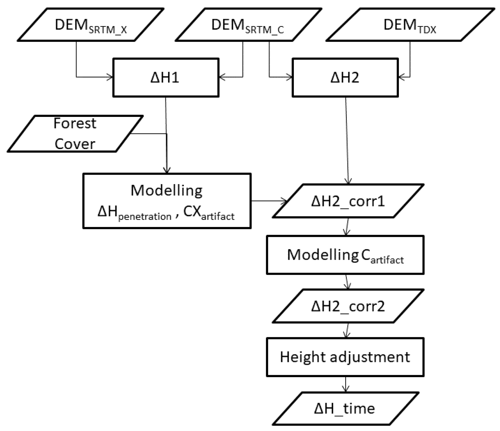
The SRTM and TanDEM-X DEMs were supplemented with a number of auxiliary datasets, all having full coverage over Uganda. We resampled the datasets to a 1-arc second spatial resolution in the WGS 84 datum and converted the SRTM DEMs to WGS 84 ellipsoidal heights. We combined the data into a stack with pixel alignment. An overview of the processing is shown in Figure 1.
2.1. Study Area
Uganda is a landlocked country with a total area of 241,551 km2, with elevation ranging from 500–5100 m a.s.l. With its location close to the Equator, the country experiences favorable rainfall and temperature and is thus endowed with diverse forest vegetation. Vegetation in natural forests can be categorized as tropical high forests and woodlands, accounting for 21 and 62% of the total forest area, respectively, and forest plantations with broadleaved and coniferous species accounting for 17% [44]. Uganda has experienced a forest loss from 3.1 million ha in the year 2000 down to 2.4 million ha in 2015. Forest losses vary greatly by management type, with a faster loss in private lands than those managed by forest and wildlife authorities [45]. Uganda has a large number of protected areas, covering 14% of the land area, and managed by either the Wildlife Authority, the National Forest Authority or district forestry services.
2.2. SRTM Data
From the SRTM mission, we used both the X- and C-band InSAR DEMs, which were acquired in February 2000 [46]. The SRTM mission acquired bi-static data by mounting SAR sensors both in the space shuttle body and on the tip of a 60-m extended boom. The C-band data were acquired with a scanSAR system of the Spaceborne Imaging Radar-C (SIR-C) hardware, while the X-band data were acquired with a strip map system. The C-band data had full areal coverage, while the X-band had partial coverage. The data were in geographic (lat/lon) projection in meters above sea level with a spatial resolution of 1 arc second. We downloaded the data as DEM tiles. The C-band data were downloaded from USGS and the X-band from the German Aerospace Centre (DLR). The tiles were mosaicked together into one C-band and one X-band DEM file over Uganda. We converted the elevation data to ellipsoidal heights using ENVI/Sarscape software. In the C-band, two small mountain areas contained void areas making up 0.24% of the country area.
2.3. TanDEM-X Data
TanDEM-X is a SAR satellite mission operating with two TerraSAR-X satellites in bistatic mode. Both satellites are operated by DLR. During their flight around the Earth, they form a crossing helix orbit, allowing them to cover the same spot from two positions [47]. The main objective of TanDEM-X is to provide data for a global DEM, the WorldDEM™, a global DEM with unprecedented accuracy [47]. However, the data are also excellent for forest monitoring applications. The satellites operate in the short wavelength, i.e., X-band, with the phase center located in the upper part of the forest canopy [48]. In the present study, we did not use the WorldDEM data as they are normally purchased, but another version having a coarser spatial resolution, i.e., 1 arc second and slightly coarser resolution in height, i.e., meters without decimals. The data were provided by Airbus Defense and Space as 37 1° × 1° tiles covering Uganda, where pixels outside Uganda were blanked. The data were given as ellipsoidal heights in WGS84-G1150 latitude/longitude projection. Each tile had been generated from a number of acquisitions, where the number varied from 13–64. The timeframe of acquisitions was from December 2010–November 2014, and we have assigned the data to one year, i.e., 2012, which represents the average year of acquisitions.
2.4. Estimating the X-C Penetration Difference
The first step was to correct for penetration difference between X- and C-band SRTM data. A part of the country was covered by SRTM X-band. Having both X- and C-band DEMs acquired here at the same point of time in the year 2000 enabled the comparison of the two DEMs and modeling of the penetration difference down into the canopy, i.e., the height difference between the X- and C-band phase centers. In order to model this, we here used Landsat-based forest cover data and estimated the penetration difference for 10% forest cover classes. A visual inspection of the difference between the X- and C-band DEMs (ΔH1) indicated a height shift, as well as artifacts in the form of line segments of about 1 km in width perpendicular to the belts that had X-band coverage (Figure 2, left). These linear features could be due to errors in the X- or C-band SRTM DEMs. We divided the belts having SRTM X-band coverage into 1 km-wide and parallel lines and assumed a fixed height error for each. We derived estimates of penetration difference between X- and C-band (ΔH_penetration) from the following models:
where Lm denoted the height shift of each artifact line segment (m = 1–1967) mentioned above. The term ΔH_penetrationn represented the penetration difference for a given 10% forest cover class (n = 0, 10%, …, 100%) (Figure 3). The final term e1 was a random error.
ΔH1 = DEMSRTM_X − DEMSRTM_C + e1
ΔH1mn = Lm + ΔH_penetrationn + e1mn
2.5. Estimating Height Changes Over Time
We derived an initial height change (ΔH2) for the time period from 2000–2012 as the difference between the TanDEM-X DEM (DEMTDX) and the SRTM C-band DEM (DEMSRTM_C).
ΔH2 = DEMTDX − DEMSRTM_C
After correcting this height change for the difference in penetration between X- and C-band, we derived a corrected height change (ΔH2_corr1).
ΔH2_corr1 = ΔH2 − ΔH_penetrationn
However, this height difference contained artifacts similar to those described above in addition to the temporal height change. The artifacts were evident from a visual inspection of the map of these height differences (Figure 4, left), appearing as parallel lines and bands, assumed to be errors in the SRTM C-band DEM in line with the findings of [43]. These lines and bands represented height errors, where all pixels of a given belt or line appeared to have a common vertical offset. The artifact pattern contained two sets of lines and two sets of belts, and we estimated a fixed height shift for each line and belt using an Analysis of Variance (ANOVA) model to make a tailored filter:
where µ was an intercept, L1i represented lines (i = 1, …, 757) of 1 km in width being parallel in the −29.8° direction; L2j was lines (j = 1, …, 535) of the same width and in the 29.6° direction; B1k was a set of belts (k = 1, …, 4) of different widths and perpendicular to L1i (60.2°); and similarly, B2l was a set of belts (l = 1, …, 4) of different widths and perpendicular to L2j (−60.4°). The directions of the lines and belts were revealed from inspection of the data; however, they could not be unambiguously and accurately determined. The e2ijkl denoted the residual error term in the ANOVA, which is assumed to be N(0,σ), and represented a further corrected height change over time (ΔH2_corr2). The intention of the ANOVA was to pick up artifacts only and leave the real temporal change in the data. We excluded pixels having large height changes by being outside the 1–99 percentile range of ΔH2_corr1, as well as pixels classified as ‘gain’ or ‘loss’ in the Global Forest Change (GFC) dataset based on a Landsat 7 ETM+ time series between 2000 and 2012 [9], leaving about 77 million pixels for the ANOVA model. The result of this modelling was not very sensitive to the selection of data to be included in the model, i.e., whether to include gain and loss pixels or not.
ΔH2_corr1ijkl = μ + L1i + L2j + B1k + B2l + e2ijkl
2.6. Vertical Bias Adjustment
We carried out a final vertical adjustment of the height difference, in order to remove a potential bias in the DEMs. We here used the median value of the ΔH2_corr2 to represent this bias. The assumption here was that there is a certain fraction of height decreases and height increases in the population of height changes and that all locations in Uganda having no height change would make up a central part of the frequency distribution. We selected the median to represent this part of the pixels. With this median (ΔH_adjust) value, we obtained the 12-year height change as:
ΔH_time = ΔH2_corr2 − ΔH_adjust
2.7. Estimating AGB and Carbon Change
We converted the height change (ΔH_time) to an estimated AGB change for every pixel. This was based on the best available conversion models. For areas with evergreen, broadleaf forest, which typically has tall trees and high biomass densities, we used a conversion model based on the relationship found between AGB from a field inventory in the same forest type in the Amani sub-mountain area in the East Usumbara mountain region in northeast Tanzania and InSAR height obtained from a TanDEM-X DEM subtracted by an airborne LiDAR DTM. Here, AGB was found to increase proportionally with InSAR height with the factor 18.4 t/ha/m [35]. There was considerable residual scattering around the AGB model, and it could not be determined whether there was a proportionality between AGB and InSAR height or whether a curve-linear model would be more appropriate. The large residual variation was likely to result mainly from small field plots, being 900 m2. When field-based AGB data were replaced by AGB estimates from airborne LiDAR, there was a clear proportionality with InSAR height and much lower residual scattering; however, this might be attributable to a saturation effect in the LiDAR model used.
For all other land cover types in Uganda, which are dominated by scattered trees and low-biomass forests, we used a model based on a study in a miombo woodland in the Liwale region, in southeast Tanzania, having similar field, TanDEM-X and airborne LiDAR data. Here, the AGB was found to increase proportionally with InSAR height with 11.9 t/ha/m [36]. It is notable that this simple proportionality model yielded a higher accuracy than an AGB model based on airborne LiDAR data. Field inventory data were available from plots of 700 m2.
We calculated the expansion from AGB to total biomass (B) using ratio values of below-ground biomass to total biomass from various literature used in draft IPCC good practice guidance for LULUCF (Land Use, Land-Use Change and Forestry) [49]. For the evergreen broadleaf forests, we used total biomass (B) = 1.24 AGB. For all other land cover types, we used B = 1.48 AGB. We further calculated total carbon as 47% of total biomass [49], which in return was converted to CO2 equivalents by multiplying with the ratio of the molecular weight of carbon dioxide to that of carbon (44/12). We did this for the entirety of Uganda, including urban areas and farmlands, assuming that trees are present also in these land cover categories. The surface height in villages and cities may change over time due to non-forest changes, e.g., due to construction of new buildings; however, these changes will cover negligible areas. Other carbon pools, i.e., soil organic carbon, dead wood and litter, might also be significant. However, we have not included these due to a lack of reliable data.
2.8. Estimation of Uncertainty and Summary Statistics
We estimated the uncertainty with Monte Carlo (MC) simulation where ΔH2 was converted through four steps as ΔH2_corr1, ΔH2_corr2, ΔH_time to finally ΔAGB. We used a random sample of 1% of the entire dataset and carried out the above sequence of processing steps for every pixel, and we did this in 100 Monte Carlo iterations. For each processing step, we allowed the relevant parameters to vary randomly according to their estimated value and the standard error of this estimate. These estimates and standard errors were derived from the GLM and ANOVA in the present study and for the conversion to ΔAGB from published values [35,36]. The Monte Carlo simulations resulted in 100 sets of data, and after aggregation, we got 100 mean values of ΔH_time and 100 mean values of ΔAGB.
From these mean values, we derived standard deviations and 95% confidence intervals, and the latter intervals were corrected for a slight deviation between the mean values of the entire dataset and the mean values of the Monte Carlo sample. We recalculated the standard deviations and confidence intervals of ΔAGB to standard deviations and confidence intervals of ΔC and ΔCO2 by scaling, and we divided the summary statistics by 12 to get annual estimates.
2.9. Comparison and Validation with External Data Sets
Ground truth data for height and biomass changes were not available for validation. However, we carried out a comparison with two sets of external data, which partly served as a validation. One set was the gain and loss dataset [9] based on Landsat data covering the same time period (2000–2012) as the present InSAR data, and the other set was three full coverage datasets of AGB over Uganda [11,12,15]. The comparisons were partly done by visual assessments of geographical patterns on maps of the data. In addition, we derived mean values of changes for the Landsat-based change categories loss, gain and no change and for land cover types. We used the land cover types from the MCD12Q1 land cover map from the U.S. Geological Survey based on MODIS data between 2001 and 2010 [50]. Ten land cover types were present in Uganda, and we reduced this to eight types by combining land cover types having a small extent. We evaluated the consistency between the InSAR height changes and Landsat based change categories. Finally, concerning the use of external, reference AGB datasets, we calculated 90, 95 and 99 percentile values. We did this for the absolute values of our estimated AGB changes and also for the external AGB stocks, and we did it separately for each land cover type. The idea behind this was that the maximum change in AGB for a given land cover type should correspond to the maximum stock in AGB for that type.
3. Results and Discussion
3.1. Estimating the X-C Penetration Difference
Linear artifacts dominated the height difference between the X- and C-band SRTM DEMs. The GLM model effectively picked up these artifacts, as well as the penetration difference between the X- and C-band in vegetation (Figure 2). The residuals of the model appeared to be random noise (Figure 2, right) with an RMSE of 2.8 m. The artifacts clearly occurred as lines across the X-band belts. The model explained 56% of the variation, and this was almost entirely attributable to linear artifacts (Table 1). The analysis of variance table is sequential, i.e., the sums of squares are obtained by entering the sources of variation sequentially.
As expected, the penetration difference increased with forest cover. However, the increase was not linear, with the largest difference found for 20% forest cover. Towards both ends of the forest cover scale, the difference was intermediate. The explanation may be that the forest cover estimation with Landsat has a problem with separating zero forest cover and complete forest cover, because these cases may appear as homogeneous areas where the contrast between forested and non-forested land is less apparent. In addition, it is possible that tall and dense grass vegetation causes a difference between the two bands in non-forest areas. We redid this modelling with separate penetration differences for different land cover types, but this had a minor influence on the results, so we discarded this.
3.2. Estimating Height Changes Over Time
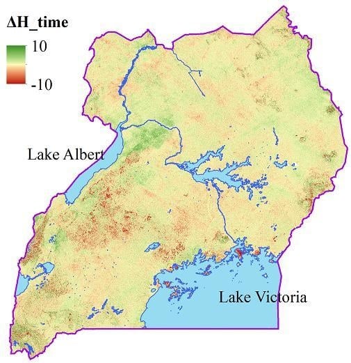
The initial height difference between the TanDEM-X and the SRTM C-band DEM (ΔH2) had pronounced artifacts similar to those described above (Figure 4). These artifacts remained when we corrected for the penetration difference between X- and C-band. The artifacts were caused by errors in the C-band SRTM DEM. We identified them with the ANOVA as clearly linear features at four different angles. The model explained 19% of the initial variance in the dataset, and the RMSE of the model was 2.2 m. The residuals of this model represented the corrected height difference (ΔH2_corr2) and appeared to represent temporal height changes more reliably. The height differences were in general smaller in magnitude, varied more smoothly over Uganda, and a number of spatial features became visible, indicating forest areas having height changes (Figure 4). The four bands going in the northeast-southwest direction were the strongest features, which alone explained 11% and by far had the highest mean square value (Table 2). These four bands largely occurred as a split of the country in two halves with a particular difference.
3.3. Vertical Bias Adjustment
The median height difference was now 0.14 m (Figure 5), which we used as an estimate of the vertical bias of the height differences. We subtracted 0.14 m from ΔH2_corr2 and obtained the final dataset representing the 12-year change in forest height (ΔH_time). The width of the 99% confidence interval of the median value was less than 1 cm. However, using this estimate for the bias and its uncertainty relies on the assumption that the median height change was an appropriate estimate of the bias between the TanDEM-X DEM and the corrected SRTM C-band DEM. This assumption represents the largest uncertainty in the results of this study, and further research on how to obtain a reliable estimate of the vertical bias would be valuable. If we assume that a considerable fraction of the land area in Uganda had no height change, then these pixels should appear as a block of data with a stable height change value in the center of the population in Figure 5. In this case, the median value would be a robust estimate of the bias, even when the number of pixels having a decrease and the number of pixels having an increase were not equal. We can see in the frequency distribution that the population of height changes had a clear peak, and not a flat top of stable height change values. However, this narrow peak can be attributable to random errors of the InSAR measurements and models applied, and not to a lack of pixels having no height change in Uganda.
3.4. Summary Statistics and Uncertainty
The mean InSAR height change for the entirety of Uganda was −7.3 cm during the years from 2000–2012 (Table 3). The standard error on this was estimated by the Monte Carlo simulation to 2.2 cm, and with a 95% confidence interval ranging from 3–11.6 cm. The input parameters for the Monte Carlo simulation are given in Table 4. This includes the penetration difference between the X- and C-band from Equation (3), the intercept and artifacts of Equation (6) and the conversion from height change to AGB change based on published models [35,36]. The estimated decrease in AGB was 1.26 ± 0.27 t/ha. The uncertainty of this decrease is underestimated, mainly because we used models based on data from smaller parts of Tanzania. However, the fact that two completely different forest types in Tanzania, i.e., the evergreen broadleaf forest and the miombo woodland, had models with parameter estimates of similar magnitude indicates that this may have a moderate influence on the uncertainty.
This corresponded to an annual carbon stock loss of 1.4 ± 0.29 Mt, with a 95% confidence interval from 0.79–1.94 Mt C. The corresponding figures for the annual emission of CO2 to the atmosphere was 5.0 ± 1.1 Mt, with a 95% confidence interval from 2.9–7.1 Mt CO2. The expansion from AGB change to CO2 change did not take into account uncertainties in the recalculation from AGB to total biomass change and, further, the conversion of this to CO2, because the uncertainties in these conversion steps were not available. These aggregated values were derived from 213 million pixels covering an area of 204,299 km2.
The Ugandan Forest Reference Level (FRL) [45] reported an annual carbon loss of 8.05 Mt/year, in CO2 equivalent, between 2000 and 2015 from deforestation and degradation after deducting a carbon gain from conservation and sustainable forest management. The difference between this and our estimate of annual carbon loss can be partially explained by differences in the approach and forest definition. In the FRL, carbon gain was estimated only from non-forest lands converted into forests. Our approach, however, accounted for non-forest conversion to forests, as well as carbon gain due to growth in forests remaining as forests. The FRL defined degradation as tropical high forests or woodlands converted into other forest types of low carbon stock, such as plantations. Our approach however accounts for carbon loss due to all forms of degradation, i.e., reduction in forest carbon due to reduction in forest height. Furthermore, unlike the FRL, the current study did not apply lower thresholds of forest definition in terms of height, forest area and crown cover parameters.
3.5. Comparison and Validation with External Datasets
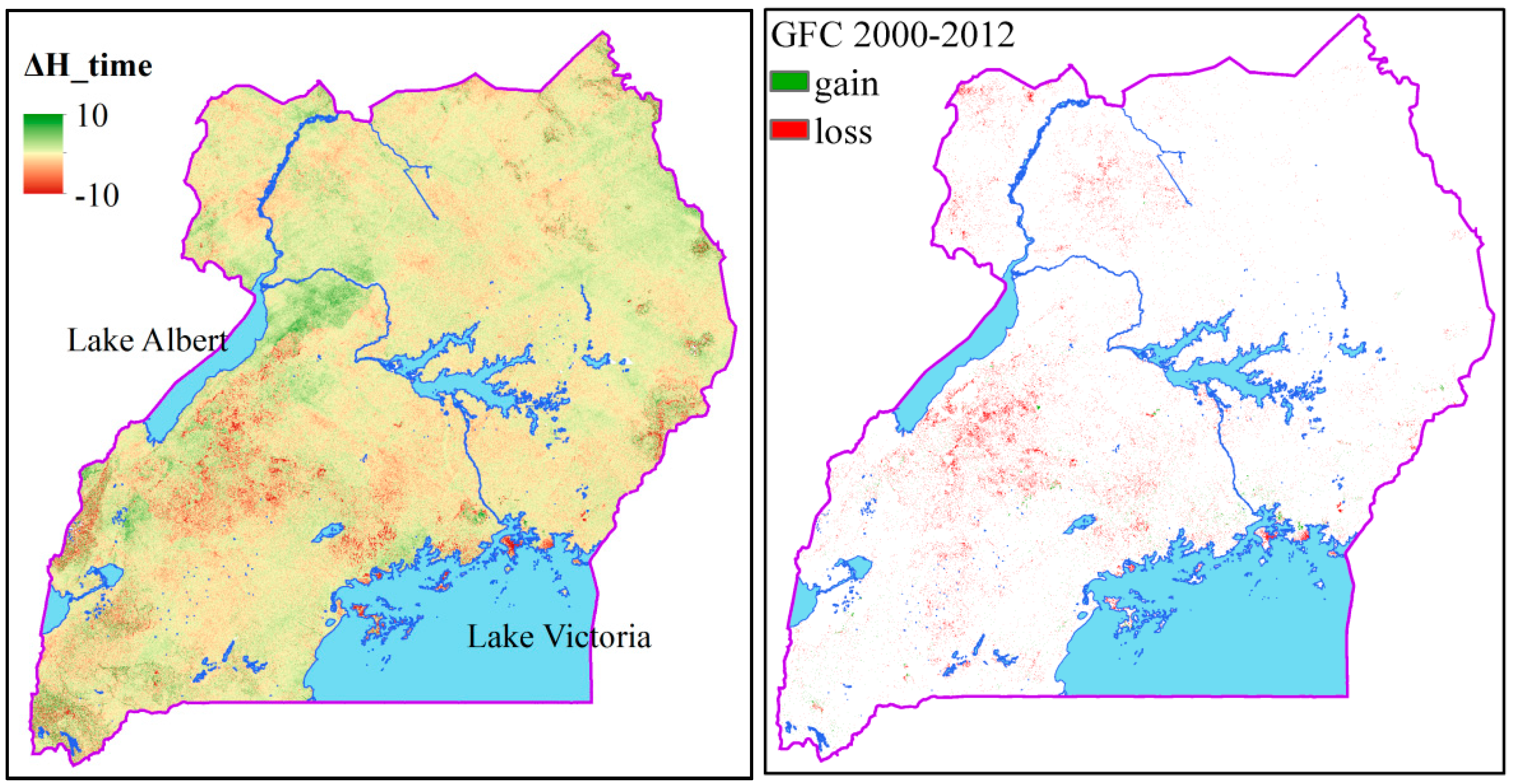
A comparison with Landsat-based change categories served as a validation of the results, while also clarifying the unique and supplementary value of the present InSAR approach. Our results show decreases in forest height occurring largely in a zone going across the country from Lake Albert in the west to Lake Victoria in the east, and being most severe in the western part (Figure 6, upper left). Increases in forest height occurred in the large Murchison Falls protected area, which is seen as a large, green area northeast of Lake Albert. Zooming up revealed a similar height increase in other protected forest areas such as Bugoma (Figure 6, lower left). There was an abrupt change from a decrease to an increase in forest height when going from the outside to the inside of the protected area, indicating an efficient protection. The changes obtained with Landsat and provided as forest gain and forest loss were generally seen in smaller fractions of the country, as compared to the other changes. The forest loss category occurred largely in the same area containing the height decreases seen with InSAR, in particular to the southeast of Lake Albert. A closer look around Bugoma also revealed a strong similarity between the InSAR- and Landsat-based decreases, which is striking when taking into account that there are two completely different measurement types. The former is based on 3D measurements of height changes, while the latter is based on spectral properties of reflected solar radiation. However, there is less similarity between InSAR and Landsat when it comes to height increases and forest gain. This is evident in the protected areas like Murchison Falls and Bugoma, where forest height apparently has increased by several meters, while no change was detected in forest cover with Landsat data. This is as expected in the case where forest cover is complete and the trees are growing in height. It is notable that the residual land sink flux of the global carbon budget, the geography and magnitude of which is largely unknown, may well occur as smaller areas and spots like the present protected areas. The obscurity of their location and magnitude may be a result of the dominance of monitoring with 2D data such as Landsat, while a 3D approach like with InSAR is required for them to be detected.
However, some SRTM errors were apparently not removed in our processing, and methods to remove such errors should be further developed. There is a narrow linear feature in the northeast-southwest direction, obviously being a remaining error. In addition, in the northern part of Uganda, some red areas are present, which appear to be erroneous due to their linear borders (Figure 6, upper left). The explanation for these features may partly be that the patterns seen are not straight linear, but rather arcs, and further studies could focus on how to identify the geometry of these arcs accurately. In addition, the linear features are likely influenced by orbit adjustments during the SRTM campaign [43] causing stripes and bands to have slightly different directions than elsewhere in the country.
The agreement between the Landsat and InSAR-based approaches, both representing the time period 2000–2012, was also demonstrated by calculating mean height changes for Landsat change categories (Table 5). For all the land cover types, the loss category had height decreases of some meters, while the no change category had mean values around zero and the gain categories had positive mean values. The mean height decrease of the loss category in the evergreen broadleaf forest type was 8.5 m, which was clearly more than the other categories, and this is reasonable as this forest type in general has very tall trees and a clear cut is expected to make up a considerable decrease in canopy height. For only one of the land cover types, i.e., grasslands, the estimated height increase for the category ‘gain’ was slightly smaller (0.2 m) than that for ‘no change’ (0.3 m). A synergistic way of combining Landsat and InSAR data is to apply such mean ΔAGB values and their corresponding CO2 emissions as local emission factors.
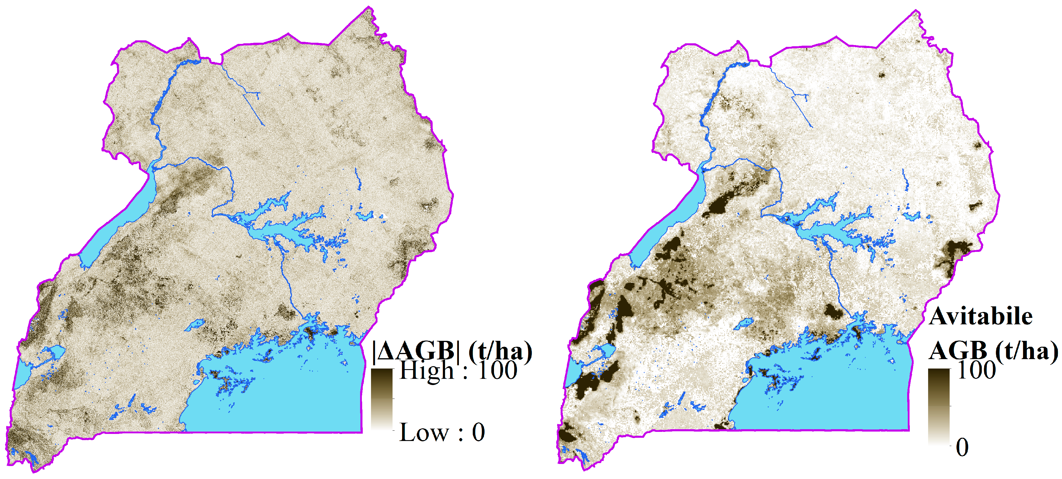
The absolute value of our estimated AGB changes varied geographically in a similar way as the AGB stocks [15]. A large magnitude of changes occurred in the western and southwestern part of Uganda and in some scattered areas including mountains around the country (Figure 7). Here, we see estimated AGB losses and increases up to about 100 t/ha or more. The same areas are seen in the map of estimated AGB stock, although the magnitude of the stocks is in general higher than the magnitude of the changes. Similar geographical patterns in AGB stocks are seen in the other published maps of AGB in Uganda [11,12]. The similarities in the magnitudes of AGB changes and AGB stocks are also evident when plotting the 99 percentile values of AGB changes for different land cover types against the corresponding 99 percentiles of published AGB stocks (Figure 8). In general, the 99 percentile values are scattered close to the 1:1 line, in particular for the Baccini [11] and Saatchi data [12]. The 99 percentile values were highly correlated with Pearson correlation coefficients above 0.9.
4. Conclusions
The presented method has a number of uncertainties that requires further research before it can be recommended as an operational method for forest monitoring. The particular SRTM biases and artifact errors need to be investigated for other and larger areas. The penetration difference between the X- and C-band in the SRTM DEMs should be studied in other forest types. The final height adjustment is crucial for the carbon change values aggregated at the national scale, as the mean forest height change is given on a cm or dm scale. The validity of a linear conversion from InSAR height change to AGB change requires more research in different forest types. However, this is an alternative and promising method as a complement to other widely-used methods today. The results corresponded well with other datasets on forest change and AGB stocks, concerning both their geographical variation and their mean and percentile values for land cover types. The next few years will provide opportunities for this approach based on the extended lifetime of TanDEM-X, expected to last until 2021, while related methods may be available through new missions like the TanDEM-L.
Acknowledgments
This study was funded by the programme on Commercialising R&D Results (FORNY2020) of The Research Council of Norway. We acknowledge Airbus Defense and Space for providing the TanDEM-X DEM.
Author Contributions
Svein Solberg carried out the statistical analyses and did the majority of the writing. Johannes May downloaded and prepared the data, Wiley Bogren contributed with data management. Johannes Breidenbach and Torfinn Torp contributed with theoretical inputs and recommendations to the uncertainty analyses. Belachew Gizachew contributed with REDD+ relevant text.
Conflicts of Interest
The authors declare no conflict of interest.
References
- Ciais, P.; Sabine, C.; Bala, G.; Bopp, L.; Brovkin, V.; Canadell, J.; Chhabra, A.; DeFries, R.; Galloway, J.; Heimann, M.; et al. Carbon and Other Biogeochemical Cycles. In Climate Change 2013: The Physical Science Basis; Stocker, T.F., Qin, D., Plattner, G.-K., Tignor, M., Allen, S.K., Boschung, J., Nauels, A., Xia, Y., Bex, V., Midgley, P.M., Eds.; Cambridge University Press: Cambridge, UK; New York, NY, USA, 2013. [Google Scholar]
- Intergovernmental Panel on Climate Change (IPCC). Climate Change 2014: Mitigation of Climate Change: IPCC Working Group III Contribution to the Fifth Assesment Report of the Intergovernmental Panel on Climate Change; Edenhofer, O., Pichs-Madruga, R., Sokona, Y., Farahani, E., Kadner, S., Seyboth, K., Adler, A., Baum, I., Brunner, S., Eickemeier, P., et al., Eds.; Cambridge University Press: Cambridge, UK; New York, NY, USA, 2014. [Google Scholar]
- UNFCCC. Decision 2/Cp. 13: Reducing Emissions from Deforestation in Developing Countries: Approaches to Stimulate Action; United Nations Framework Convention on Climate Chgange: Bonn, Germany, 2007; Available online: http://Unfccc.Int/Resource/Docs/2007/Cop13/Eng/06a01.Pdf (accessed on 19 September 2014).
- Decision 4/Cp.15. Methodological Guidance for Activities Relating to Reducing Emissions from Deforestation and Forest Degradation and the Role of Conservation, Sustainable Management of Forests and Enhancement of Forest Carbon Stocks in Developing Countries; United Nations Framework Convention on Climate Change: Bonn, Germany, 2009; Available online: http://Unfccc.Int/Resource/Docs/2009/Cop15/Eng/11a01.Pdf (accessed on 19 September 2014).
- Quéré, C.L.; Moriarty, R.; Andrew, R.M.; Canadell, J.G.; Sitch, S.; Korsbakken, J.I.; Friedlingstein, P.; Peters, G.P.; Andres, R.J.; Boden, T.A.; et al. Global Carbon Budget 2015. Earth Syst. Sci. Data 2015, 7, 349–396. [Google Scholar] [CrossRef] [Green Version]
- Houghton, R.A.; House, J.I.; Pongratz, J.; Van Der Werf, G.R.; DeFries, R.S.; Hansen, M.C.; Quere, C.L.; Ramankutty, N. Carbon Emissions from Land Use and Land-Cover Change. Biogeosciences 2012, 9, 5125–5142. [Google Scholar] [CrossRef]
- MacDicken, K.G. Global Forest Resources Assessment 2015: What, Why and How? For. Ecol. Manag. 2015, 352, 3–8. [Google Scholar] [CrossRef]
- Pan, Y.D.; Birdsey, R.A.; Fang, J.Y.; Houghton, R.; Kauppi, P.E.; Kurz, W.A.; Phillips, O.L.; Shvidenko, A.; Lewis, S.L.; Canadell, J.G.; et al. A Large and Persistent Carbon Sink in the World’s Forests. Science 2011, 333, 988–993. [Google Scholar] [CrossRef] [PubMed]
- Hansen, M.C.; Potapov, P.V.; Moore, R.; Hancher, M.; Turubanova, S.A.; Tyukavina, A.; Thau, D.; Stehman, S.V.; Goetz, S.J.; Loveland, T.R.; Kommareddy, A.; et al. High-Resolution Global Maps of 21st-Century Forest Cover Change. Science 2013, 342, 850–853. [Google Scholar] [CrossRef] [PubMed]
- Hansen, M.C.; Shimabukuro, Y.E.; Potapov, P.; Pittman, K. Comparing Annual MODIS and Prodes Forest Cover Change Data for Advancing Monitoring of Brazilian Forest Cover. Remote Sens. Environ. 2008, 112, 3784–3793. [Google Scholar] [CrossRef]
- Baccini, A.; Goetz, S.J.; Walker, W.S.; Laporte, N.T.; Sun, M.; Sulla-Menashe, D.; Hackler, J.; Beck, P.S.A.; Dubayah, R.; Friedl, M.A.; et al. Estimated Carbon Dioxide Emissions from Tropical Deforestation Improved by Carbon-Density Maps. Nat. Clim. Chang. 2012, 2, 182–185. [Google Scholar] [CrossRef]
- Saatchi, S.S.; Harris, N.L.; Brown, S.; Lefsky, M.; Mitchard, E.T.A.; Salas, W.; Zutta, B.R.; Buermann, W.; Lewis, S.L.; Hagen, S.; et al. Benchmark Map of Forest Carbon Stocks in Tropical Regions across Three Continents. Proc. Natl. Acad. Sci. USA 2011, 108, 9899–9904. [Google Scholar] [CrossRef] [PubMed]
- Avitabile, V.; Baccini, A.; Friedl, M.A.; Schmullius, C. Capabilities and Limitations of Landsat and Land Cover Data for Aboveground Woody Biomass Estimation of Uganda. Remote Sens. Environ. 2012, 117, 366–380. [Google Scholar] [CrossRef]
- Mitchard, E.T.A.; Feldpausch, T.R.; Brienen, R.J.W.; Lopez-Gonzalez, G.; Monteagudo, A.; Baker, T.R.; Lewis, S.L.; Lloyd, J.; Quesada, C.A.; Gloor, M.; et al. Markedly Divergent Estimates of Amazon Forest Carbon Density from Ground Plots and Satellites. Glob. Ecol. Biogeogr. 2014, 23, 935–946. [Google Scholar] [CrossRef] [PubMed] [Green Version]
- Avitabile, V.; Herold, M.; Henry, M.; Schmullius, C. Mapping Biomass with Remote Sensing: A Comparison of Methods for the Case Study of Uganda. Carbon Balance Manag. 2011, 6, 7. [Google Scholar] [CrossRef] [PubMed]
- Næsset, E. Predicting Forest Stand Characteristics with Airborne Scanning Laser Using a Practical Two-Stage Procedure and Field Data. Remote Sens. Environ. 2002, 80, 88–99. [Google Scholar] [CrossRef]
- Persson, H. Estimation of Boreal Forest Attributes from Very High Resolution Pléiades Data. Remote Sens. 2016, 8, 736. [Google Scholar] [CrossRef]
- Karjalainen, M.; Kankare, V.; Vastaranta, M.; Holopainen, M.; Hyyppa, J. Prediction of Plot-Level Forest Variables Using Terrasar-X Stereo Sar Data. Remote Sens. Environ. 2012, 117, 338–347. [Google Scholar] [CrossRef]
- Treuhaft, R.N.; Madsen, S.N.; Moghaddam, M.; Zyl, J.J. Vegetation Characteristics and Underlying Topography from Interferometric Radar. Radio Sci. 1996, 31, 1449–1485. [Google Scholar] [CrossRef]
- Treuhaft, R.N.; Siqueira, P.R. Vertical Structure of Vegetated Land Surfaces from Interferometric and Polarimetric Radar. Radio Sci. 2000, 35, 141–177. [Google Scholar] [CrossRef]
- Askne, J.I.H.; Dammert, P.B.G.; Ulander, L.M.H.; Smith, G. C-Band Repeat-Pass Interferometric Sar Observations of the Forest. IEEE Trans. Geosci. Remote Sens. 1997, 35, 25–35. [Google Scholar] [CrossRef]
- Soja, M.J.; Persson, H.; Ulander, L.M.H. Estimation of Forest Height and Canopy Density from a Single Insar Correlation Coefficient. IEEE Geosci. Remote Sens. Lett. 2015, 12, 646–650. [Google Scholar] [CrossRef]
- Soja, M.J.; Persson, H.J.; Ulander, L.M. Estimation of Forest Biomass from Two-Level Model Inversion of Single-Pass Insar Data. IEEE Trans. Geosci. Remote Sens. 2015, 53, 5083–5099. [Google Scholar] [CrossRef]
- Treuhaft, R.; Lei, Y.; Gonçalves, F.; Keller, M.; Santos, J.; Neumann, M.; Almeida, A. Tropical-Forest Structure and Biomass Dynamics from Tandem-X Radar Interferometry. Forests 2017, 8, 277. [Google Scholar] [CrossRef]
- Kellndorfer, J.; Walker, W.; Pierce, L.; Dobson, C.; Fites, J.A.; Hunsaker, C.; Vona, J.; Clutter, M. Vegetation Height Estimation from Shuttle Radar Topography Mission and National Elevation Datasets. Remote Sens. Environ. 2004, 93, 339–358. [Google Scholar] [CrossRef]
- Kenyi, L.W.; Dubayah, R.; Hofton, M.; Schardt, M. Comparative Analysis of Srtm-Ned Vegetation Canopy Height to Lidar-Derived Vegetation Canopy Metrics. Int. J. Remote Sens. 2009, 30, 2797–2811. [Google Scholar] [CrossRef]
- Sexton, J.O.; Bax, T.; Siqueira, P.; Swenson, J.J.; Hensley, S. A Comparison of Lidar, Radar, and Field Measurements of Canopy Height in Pine and Hardwood Forests of Southeastern North America. For. Ecol. Manag. 2009, 257, 1136–1147. [Google Scholar] [CrossRef]
- Solberg, S.; Astrup, R.; Bollandsas, O.M.; Naesset, E.; Weydahl, D.J. Deriving Forest Monitoring Variables from X-Band Insar Srtm Height. Can. J. Remote Sens. 2010, 36, 68–79. [Google Scholar] [CrossRef]
- Ni, W.; Guo, Z.; Sun, G.; Chi, H. Investigation of Forest Height Retrieval Using Srtm-Dem and Aster-Gdem. Presented at the International Geoscience and Remote Sensing Symposium (IGARSS), Honolulu, HI, USA, 25–30 July 2010. [Google Scholar]
- Solberg, S.; Astrup, R.; Breidenbach, J.; Nilsen, B.; Weydahl, D. Monitoring Spruce Volume and Biomass with Insar Data from Tandem-X. Remote Sens. Environ. 2013, 139, 60–67. [Google Scholar] [CrossRef]
- Solberg, S.; Astrup, R.; Weydahl, D.J. Detection of Forest Clear-Cuts with Shuttle Radar Topography Mission (Srtm) and Tandem-X Insar Data. Remote Sens. 2013, 5, 5449–5462. [Google Scholar] [CrossRef]
- Woodhouse, I.H. Predicting Backscatter-Biomass and Height-Biomass Trends Using a Macroecology Model. IEEE Trans. Geosci. Remote Sens. 2006, 44, 871–877. [Google Scholar] [CrossRef]
- Neeff, T.; Dutra, L.V.; Dos Santos, J.R.; Freitas, C.D.; Araujo, L.S. Tropical Forest Measurement by Interferometric Height Modeling and P-Band Radar Backscatter. For. Sci. 2005, 51, 585–594. [Google Scholar]
- Gama, F.F.; Dos Santos, J.R.; Mura, J.C. Eucalyptus Biomass and Volume Estimation Using Interferometric and Polarimetric Sar Data. Remote Sens. 2010, 2, 939–956. [Google Scholar] [CrossRef]
- Solberg, S.; Hansen, E.H.; Gobakken, T.; Næssset, E.; Zahabu, E. Biomass and Insar Height Relationship in a Dense Tropical Forest. Remote Sens. Environ. 2017, 192, 166–175. [Google Scholar] [CrossRef]
- Puliti, S.; Solberg, S.; Næsset, E.; Gobakken, T.; Zahabu, E.; Mauya, E.; Malimbwi, R.E. Modelling above Ground Biomass in Tanzanian Miombo Woodlands Using Tandem-X Worlddem and Field Data. Remote Sens. 2017, 9, 984. [Google Scholar] [CrossRef]
- Solberg, S.; Næsset, E.; Gobakken, T.; Bollandsås, O.M. Forest Biomass Change Estimated from Height Change in Interferometric Sar Height Models. Carbon Balance Manag. 2014, 9, 5. [Google Scholar] [CrossRef] [PubMed]
- Solberg, S.; Weydahl, D.J.; Astrup, R. Temporal Stability of X-Band Single-Pass Insar Heights in a Spruce Forest: Effects of Acquisition Properties and Season. IEEE Trans. Geosci. Remote Sens. 2015, 53, 1607–1614. [Google Scholar] [CrossRef]
- Solberg, S.; Lohne, T.P.; Karyanto, O. Temporal Stability of Insar Height in a Tropical Rainforest. Remote Sens. Lett. 2015, 6, 209–217. [Google Scholar] [CrossRef]
- Praks, J.; Demirpolat, C.; Antropov, O.; Hallikainen, M. On Forest Height Retrival from Spaceborne X-Band Inferometic Sar Images under Variable Seasonal Conditions. In Proceedings of the XXXII Finnish URSI Convention on Radio Science and SMARAD Seminar, Otaniemi, Finland, 24–25 April 2013; pp. 115–118. [Google Scholar]
- Way, J.; Paris, J.; Kasischke, E.; Slaughter, C.; Viereck, L.; Christensen, N.; Dobson, M.C.; Ulaby, F.; Richards, J.; Milne, A.; et al. The Effect of Changing Environmental-Conditions on Microwave Signatures of Forest Ecosystems: Preliminary Results of the March 1988 Alaskan Aircraft Sar Experiment. Int. J. Remote Sens. 1990, 11, 1119–1144. [Google Scholar] [CrossRef]
- Hoffmann, J.; Walter, D. How Complementary Are Srtm-X and -C Band Digital Elevation Models? Photogramm. Eng. Remote Sens. 2006, 72, 261–268. [Google Scholar] [CrossRef]
- Walker, W.S.; Kellndorfer, J.M.; Pierce, L.E. Quality Assessment of Srtm C- and X-Band Interferometric Data: Implications for the Retrieval of Vegetation Canopy Height. Remote Sens. Environ. 2007, 106, 428–448. [Google Scholar] [CrossRef]
- Drichi, P. National Biomass Study Technical Report 1996–2002; Kampala, Forest Department, Ministry of Water, Lands and Environment: Kampala, Uganda, 2002.
- MoWE. Proposed Forest Reference Level for Uganda; Republic of Uganda Ministry of Water and Environment: Kampala, Uganda, 2017. Available online: http://Redd.Unfccc.Int/Files/Uganda_Frel_Final_Version_16.01.Pdf (accessed on 23 August 2017).
- Rabus, B.; Eineder, M.; Roth, A.; Bamler, R. The Shuttle Radar Topography Mission—A New Class of Digital Elevation Models Acquired by Spaceborne Radar. ISPRS J. Photogramm. Remote Sens. 2003, 57, 241–262. [Google Scholar] [CrossRef]
- Krieger, G.; Moreira, A.; Fiedler, H.; Hajnsek, I.; Werner, M.; Younis, M.; Zink, M. Tandem-X: A Satellite Formation for High-Resolution Sar Interferometry. IEEE Trans. Geosci. Remote Sens. 2007, 45, 3317–3341. [Google Scholar] [CrossRef] [Green Version]
- Chen, Y.; Shi, P.; Deng, L.; Li, J. Generation of a Top-of-Canopy Digital Elevation Model (DEM) in Tropical Rain Forest Regions Using Radargrammetry. Int. J. Remote Sens. 2007, 28, 4345–4349. [Google Scholar] [CrossRef]
- Intergovernmental Panel on Climate Change (IPCC). Guidelines for National Greenhouse Gas Inventories: Volume 4: Agriculture, Forestry and Other Land Use; Institute for Global Environmental Strategies: Kanagawa Prefecture, Japan, 2006. [Google Scholar]
- Friedl, M.A.; Sulla-Menashe, D.; Tan, B.; Schneider, A.; Ramankutty, N.; Sibley, A.; Huang, X. MODIS Collection 5 Global Land Cover: Algorithm Refinements and Characterization of New Datasets, 2001–2012; Collection 5.1 Igbp Land Cover; Boston University: Boston, MA, USA, 2010. [Google Scholar]
Figure 1.
Flowchart for estimating temporal change in X-band InSAR elevation in Uganda (ΔH_time).

Figure 2.
The height difference between the X- and C-band SRTM DEMs (left), the linear artifacts predicted by the GLM model (middle) and the residual noise (right).
Figure 2.
The height difference between the X- and C-band SRTM DEMs (left), the linear artifacts predicted by the GLM model (middle) and the residual noise (right).

Figure 3.
The effect of forest cover on the penetration difference between the X- and C-band SRTM DEMs.
Figure 3.
The effect of forest cover on the penetration difference between the X- and C-band SRTM DEMs.

Figure 4.
Map of Uganda with the height difference between the TanDEM-X DEM and the C-band SRTM DEM (left), the predicted errors identified by the ANOVA representing the line and belt artifacts of the SRTM C-band DEM (middle) and the residuals from the ANOVA representing ΔH2_corr2.
Figure 4.
Map of Uganda with the height difference between the TanDEM-X DEM and the C-band SRTM DEM (left), the predicted errors identified by the ANOVA representing the line and belt artifacts of the SRTM C-band DEM (middle) and the residuals from the ANOVA representing ΔH2_corr2.

Figure 5.
Frequency distribution of height differences (ΔH2_corr2) within its 1–99 percentile range.
Figure 5.
Frequency distribution of height differences (ΔH2_corr2) within its 1–99 percentile range.

Figure 6.
Changes in forest height based on InSAR DEMs (left) and in forest cover based on Landsat (right) from 2000–2012 [9], where the upper panels show results for the entirety Uganda and lower panels for an area around the Bugoma protected forest in the western part. The white areas in the right panels represent no change.


Figure 7.
Maps of the absolute value of ΔAGB (left) and AGB based on [15].
Figure 7.
Maps of the absolute value of ΔAGB (left) and AGB based on [15].

Figure 8.
The 99th percentile of ΔAGB for seven land cover classes plotted against the corresponding 99th percentile of the AGB stocks based on [11,12,15]. The land cover types are given as labels for the points of [15], where the numbers correspond to land cover types as given in Table 5.


Table 1.
Analyses of variance of the GLM model of ΔH1 (m) (Equation (3)). The model had an R2 of 56%.
Table 1.
Analyses of variance of the GLM model of ΔH1 (m) (Equation (3)). The model had an R2 of 56%.
| Source | DF | Sum of Squares | Mean Square |
|---|---|---|---|
| Artifact lines, Lm | 1966 | 678,972,490 | 345,357 |
| ΔH_penetration | 10 | 1,553,541 | 155,354 |
| Error, e1 | 68,309,116 | 540,543,128 | 8 |
| Corrected Total | 68,311,092 | 1,221,069,159 |
Table 2.
Results of the analyses of variance (ANOVA) for removing artifact lines and bands of the SRTM C-band DEM (m) (Equation (6)). The model had an R2 of 19%.
Table 2.
Results of the analyses of variance (ANOVA) for removing artifact lines and bands of the SRTM C-band DEM (m) (Equation (6)). The model had an R2 of 19%.
| Source | DF | Sum of Squares | Mean Square |
|---|---|---|---|
| Artifact lines, L1i | 756 | 16,031,767 | 21,206 |
| Artifact lines, L2j | 534 | 17,213,609 | 32,235 |
| Artifact bands, B1k | 3 | 46,665,641 | 15,555,214 |
| Artifact bands, B2l | 3 | 2,378,282 | 792,761 |
| Error, e2 | 76,153,436 | 361,137,038 | 5 |
| Corrected Total | 76,154,732 | 443,426,337 |
Table 3.
Summary statistics and uncertainty for ΔH_time and ΔAGB. The mean is derived from the entire population, while the standard error of the mean (SE) and the 95% confidence intervals (CI) are derived from 100 Monte Carlo iterations based on a subsample of 1% of the dataset and rescaled to the mean.
| Source | Mean | SE | Lower 95% CI | Upper 95% CI |
|---|---|---|---|---|
| ΔH_time | −0.073 | 0.022 | −0.116 | −0.030 |
| ΔAGB | −1.26 | 0.27 | −1.79 | −0.73 |
Table 4.
The 7 input parameters for the Monte Carlo simulation, with the number of parameter values (N), their mean and min-max and the mean and min-max of their standard errors.
Table 4.
The 7 input parameters for the Monte Carlo simulation, with the number of parameter values (N), their mean and min-max and the mean and min-max of their standard errors.
| Parameter | N | Mean | Min | Max | SE_mean | SE_min | SE_max |
|---|---|---|---|---|---|---|---|
| Penetration XC | 11 | −0.368 | −0.799 | 0.205 | 0.00354 | 0.00000 | 0.00522 |
| Intercept | 1 | 0.00513 | - | - | 0.208 | - | - |
| L1 | 757 | 0.437 | −0.897 | 1.710 | 0.0607 | 0.0000 | 0.0921 |
| L2 | 535 | −1.61 | −3.92 | 0.500 | 0.200 | 0.000 | 0.659 |
| B1 | 4 | −0.921 | −1.32 | 0.000 | 0.00162 | 0.00000 | 0.00348 |
| B2 | 4 | 0.541 | 0.000 | 1.22 | 0.00204 | 0.00000 | 0.00349 |
| AGB | 2 | 11.90 | 18.40 | 24.1 | 203 |
Table 5.
Mean height change and corresponding AGB change for combinations of land cover type and Landsat-based gain-loss categories.
Table 5.
Mean height change and corresponding AGB change for combinations of land cover type and Landsat-based gain-loss categories.
| No. | MODIS Land Cover Type | ΔH_Time, m | ΔAGB, t/ha | ||||
|---|---|---|---|---|---|---|---|
| Loss | No Change | Gain | Loss | No Change | Gain | ||
| 2 | Evergreen broadleaf forest | −8.5 | −0.7 | 1.0 | −156.3 | −12.9 | 18.0 |
| 8 | Woody savanna | −3.3 | 0.4 | 1.2 | −39.3 | 4.8 | 13.8 |
| 9 | Savanna | −1.3 | −0.1 | 1.9 | −15.0 | −0.9 | 22.1 |
| 10 | Grassland | −1.5 | 0.3 | 0.2 | −18.4 | 3.7 | 2.8 |
| 11 | Permanent wetlands | −3.0 | 0.5 | 0.6 | −36.0 | 6.5 | 7.0 |
| 12 | Croplands | −1.2 | 0.2 | 1.4 | −14.3 | 2.9 | 16.3 |
| 14 | Cropland and natural vegetation mosaic | −3.6 | −0.1 | 1.5 | −42.6 | −1.3 | 17.3 |
| Others | −3.7 | 0.7 | 1.5 | −44.5 | 8.3 | 17.7 | |
© 2018 by the authors. Licensee MDPI, Basel, Switzerland. This article is an open access article distributed under the terms and conditions of the Creative Commons Attribution (CC BY) license (http://creativecommons.org/licenses/by/4.0/).
Share and Cite
MDPI and ACS Style
Solberg, S.; May, J.; Bogren, W.; Breidenbach, J.; Torp, T.; Gizachew, B. Interferometric SAR DEMs for Forest Change in Uganda 2000–2012. Remote Sens. 2018, 10, 228. https://doi.org/10.3390/rs10020228
AMA Style
Solberg S, May J, Bogren W, Breidenbach J, Torp T, Gizachew B. Interferometric SAR DEMs for Forest Change in Uganda 2000–2012. Remote Sensing. 2018; 10(2):228. https://doi.org/10.3390/rs10020228
Chicago/Turabian StyleSolberg, Svein, Johannes May, Wiley Bogren, Johannes Breidenbach, Torfinn Torp, and Belachew Gizachew. 2018. "Interferometric SAR DEMs for Forest Change in Uganda 2000–2012" Remote Sensing 10, no. 2: 228. https://doi.org/10.3390/rs10020228
Note that from the first issue of 2016, this journal uses article numbers instead of page numbers. See further details here.