An Optimal Tropospheric Tomography Method Based on the Multi-GNSS Observations

Abstract

Aside from the well-known applications (positioning, navigation and timing) brought by Global Navigation Satellite System (GNSS), reconstruction of tropospheric atmosphere distribution information using tomography technique based on the multi-GNSS observations has been developed as a research point in the fields of GNSS Meteorology. In this paper, an optimal tropospheric tomography method using observations from multi-GNSS (Global Navigation Satellite System) is proposed, which considers the reasonable weightings of observation equations derived from multi-GNSS as well as the various constraints. Comparing to the equal weighting strategy of multi-GNSS observations for the previously multi-GNSS tomography studies, the proposed method in this paper has the ability to tune the weightings for a different type of equations. Experiments show that the proposed method can improve the internal/external accuracy of GNSS tomography modeling with the GNSS precise point positioning (PPP)-estimated slant wet delay as reference when compared to the conventional method. In addition, the data derived from radiosonde is used as an external testing, and the result also expresses the superiority of the proposed method when compared to the conventional method.

1. Introduction

Since the tomography technique is proposed by [1] for exploring the possibility to calculate the density distribution of an object using the X-ray projections, its application has first been used in the medicinal field by [2]. After that, such technique became a popular and powerful tool to describe the spatial-temporal distribution of the parameters of the interested area in many areas like geology [3,4,5]. In the troposphere area, the conception of reconstruction of troposphere water vapor information were pointed out by [6] using twenty ground-based GPS (Global Positioning System) stations from the local network. The application of troposphere tomography technique was first realized and verified its accuracy by [7].

Usually, the troposphere tomographic area was discretized into many voxels and with the assumption that the value of each voxel is a constant for a given period. Therefore, the Global Navigation Satellite System (GNSS) signal ray that crossed those voxels can be used to build the observation equation for tomography modeling [8,9]. However, subjecting to the geometric distribution of GNSS satellite constellations and the unfavorable geometry of ground-based GNSS stations in a network, many voxels cannot be crossed by any ray during the tomography period. Consequently, this will result in a problem of rank deficiency [10]. To solve such ill-posed issue, some constraints (horizontal and vertical constraints) are needed to impose onto the tomography modeling [11,12,13,14]. [15] proposed a tomography method using the adaptive smoothing and ground meteorological observations, which improves the tomographic result in the lower troposphere.

With the increasing improvement of multi-GNSS, especially for BDS (BeiDou navigation satellite system), GLONASS satellite system and Galileo, more satellite rays can be used for establishing the tomography observation modeling, which is favorable for the multi-GNSS troposphere tomography. [16] have analyzed the accuracy of tomography results using the simulated data from three satellite systems (GPS, GLONASS and Galileo) and verified its improvement over that of the single GPS system. [17] also obtained similar results using the simulated data from BDS and GPS system. [18] found that, in some epochs, the additional Galileo observations do not have a positive impact in the tomography solution based on the simulated GPS and Galileo data. [19] obtained the three-dimensional water vapor in Wuhan using GPS, BDS and GLONASS observations with the Multiplicative Algebraic Reconstruction Technique (MART) method. However, two points need to be noted that: (1) only the simulated data was used to perform the multi-GNSS tropospheric tomography; and (2) the weightings for different satellite systems as well as the various constraints were not considered before. Therefore, an optimal tropospheric tomography method based on the Multi-GNSS Observations is proposed, while considering the weightings of different input information for establishing the tomography modeling. In this paper, the observed data from multi-GNSS (GPS, GLONASS and BDS) was used to establish the observation equation, and the horizontal, vertical and prior constraints were also introduced. In addition, the improved Bartlett test was used to determine the optimal weightings of different input information of tomography modeling by adjusting their posterior unit weight variances.

2. Tomography Theory and Method

2.1. Establishment of Tropospheric Tomography Modeling

It is well known that the zenith total delay (ZTD) is an average parameter in spatial aspects, and some important information about the local variability of the atmosphere is lost. In fact, ZTD is an integral parameter, and the information about the vertical structure of the atmosphere is lost [20]. The zenith wet delay (ZWD) can be extracted from ZTD by removing the zenith hydrostatic delay (ZHD) calculated using the Saastamoinen model [21]. Therefore, the SWD (Slant wet delay) can be obtained by projecting the ZWD value to the slant path, which is regarded as the input information of GNSS troposphere tomography modeling.

According to the distances of GNSS rays calculated in each divided voxel of the tomography area and the unknown wet refractivity to be estimated, the observation equation of troposphere tomography can be expressed as:

$$SWD={\displaystyle \sum d_{ijk}\cdot x_{ijk}},$$

(1)

where the subscripts of ($i,j,k$) represent the location of voxels in horizontal and vertical directions. $d$ is the distance of satellite ray in the voxel ($i,j,k$), while $x$ is the unknown parameters to be estimated in the voxel ($i,j,k$).

As mentioned before, some empirical constraints are considered to overcome the rank deficiency problem. For the small tomography area, a certain voxel can be described by the weighted value of its neighbors horizontally [22]. The relative horizontal constraint can be unified expressed as follows:

$$h_1\cdot x_1+h_2\cdot x_2+\cdots +h_{m-1}\cdot x_{m-1}-x_m+h_{m+1}\cdot x_{m+1}+\cdots +h_n\cdot x_n=0,$$

(2)

where $h$ is the horizontal weighted coefficient while $n$ is the total number of voxels in the same layer.

The vertical constraint is constructed based on the exponential function in different layers as follows [23,24]:

$$x_i=x_{i-1}\cdot e^{(h_{i-1}-h_i)/H},$$

(3)

where $x_i$ and $h_i$ are the wet refractivity value and the corresponding height of the voxel $i$, respectively. $H$ denotes the water vapor scale height, which ranges from 1 to 2 km.

Aside from horizontal and vertical constraints, an a priori constraint is also imposed for the location of radiosonde station using the mean value of radiosonde data in the first three days before the tomography epoch. The priori constraint can be described as follows:

$$x_q=x_{0_q}^{rs},$$

(4)

where $x_0^{rs}$ represents the initial wet refractivity value calculated using the radiosonde data in the first three days before the tomography epoch. $q$ is equal to the number of vertical layers of the tomography area.

Due to the data from multi-GNSS (GPS, GLONASS and BDS) being used in our study, the final tomography modeling can thus be expressed as follows:

$$\left[\begin{array}{l}{\mathbf{y}}_{m1\times 1}^{gps}\\ {\mathbf{y}}_{m2\times 1}^{glonass}\\ {\mathbf{y}}_{m3\times 1}^{bds}\\ {\mathbf{y}}_{m4\times n1}^H\\ {\mathbf{y}}_{m5\times n1}^V\\ {\mathbf{y}}_{m6\times 1}^P\end{array}\right]=\left[\begin{array}{l}{\mathbf{A}}_{m1\times n1}^{gps}\\ {\mathbf{A}}_{m2\times n1}^{glonass}\\ {\mathbf{A}}_{m3\times n1}^{bds}\\ {\mathbf{A}}_{m4\times n1}^H\\ {\mathbf{A}}_{m5\times n1}^V\\ {\mathbf{A}}_{m6\times n1}^P\end{array}\right]\cdot {\mathbf{X}}_{n1\times 1}+\left[\begin{array}{l}{\mathbf{\Delta }}_{m1\times 1}^{gps}\\ {\mathbf{\Delta }}_{m2\times 1}^{glonass}\\ {\mathbf{\Delta }}_{m3\times 1}^{bds}\\ {\mathbf{\Delta }}_{m4\times 1}^H\\ {\mathbf{\Delta }}_{m5\times 1}^V\\ {\mathbf{\Delta }}_{m6\times 1}^P\end{array}\right],$$

(5)

where ${\mathbf{y}}^{tp1}$, ${\mathbf{A}}^{tp1}$ and ${\mathbf{\Delta }}^{tp1}$ ($tp1=\mathit{gps},\mathit{glonass},\mathit{bds}$) represent the column vectors with a set of SWD observations derived from multi-GNSS (GPS, GLONASS and BDS), the design matrices with the value of the distance of the satellite ray inside a certain voxel and the noise of the multi-GNSS observation equations, respectively. ${\mathbf{y}}^{tp2}$ ($tp2=H,V,P$) represents the column vectors with the value of 0 for horizontal and vertical constraints while the value for priori constraint is calculated using radiosonde data in the first three days before tomography epoch. ${\mathbf{A}}^{tp2}$ represents the coefficient matrices of horizontal, vertical and priori constraints while ${\mathbf{\Delta }}^{tp2}$ represents the noise of the different constraint equations. $mi$ ($i=1,2,\cdots ,5,6$) represents the number of six equations while $n1$ denotes the number of unknown parameters to be estimated.

Assuming that the covariance matrices for different inputs are ${\mathbf{D}}^{tp}$ ($tp=\mathit{gps},\mathit{glonass},\mathit{bds},H,V,P$), which can be described as follows:

$$\begin{array}{ll}{\mathbf{D}}^{tp}& =\mathrm{diag}({\mathbf{D}}^{gps},{\mathbf{D}}^{glonass},{\mathbf{D}}^{bds},{\mathbf{D}}^H,{\mathbf{D}}^V,{\mathbf{D}}^P)\\ & =\mathrm{diag}({\mathsf{\sigma }}_{0_{gps}}^2,{\mathsf{\sigma }}_{0_{glonass}}^2,{\mathsf{\sigma }}_{0_{gps}}^2,{\mathsf{\sigma }}_{0_H}^2,{\mathsf{\sigma }}_{0_V}^2,{\mathsf{\sigma }}_{0_P}^2)\cdot \mathrm{diag}({\mathbf{P}}_{gps}^{-1},{\mathbf{P}}_{glonass}^{-1},{\mathbf{P}}_{bds}^{-1},{\mathbf{P}}_H^{-1},{\mathbf{P}}_V^{-1},{\mathbf{P}}_P^{-1})\end{array},$$

(6)

where ${\mathsf{\sigma }}_{0_{tp}}^2$ and ${\mathbf{P}}_{tp}^{-1}$ ($tp=\mathit{gps},\mathit{glonass},\mathit{bds},H,V,P$) denote the variances of unit weight and the weight matrices for the six types of equations, respectively.

2.2. Optimal Solution Strategy for Multi-GNSS Troposphere Tomography Modeling

As described in Section 2.1, the final unknown parameter can be estimated based on Equations (5) and (6):

$$\widehat{\mathbf{X}}={\left({\displaystyle \sum {\mathbf{A}}_{\mathrm{tp}1}^T\cdot {\mathbf{P}}_{\mathrm{tp}1}^T\cdot {\mathbf{A}}_{\mathrm{tp}1}^{}+{\displaystyle \sum {\mathbf{A}}_{\mathrm{tp}2}^T\cdot {\mathbf{P}}_{\mathrm{tp}2}^T\cdot {\mathbf{A}}_{\mathrm{tp}2}^{}}}\right)}^{-1}\cdot \left({\displaystyle \sum {\mathbf{A}}_{\mathrm{tp}1}^T\cdot {\mathbf{P}}_{\mathrm{tp}1}^T\cdot {\mathbf{y}}_{\mathrm{tp}1}^{}+{\displaystyle \sum {\mathbf{A}}_{\mathrm{tp}2}^T\cdot {\mathbf{P}}_{\mathrm{tp}2}^T\cdot {\mathbf{y}}_{\mathrm{tp}2}^{}}}\right).$$

(7)

Usually, the unit weight variances for different types of equations are regarded as the same value. Due to the fact that the troposphere tomography modeling is established using different types of multi-GNSS observations as well as various constraints, it is therefore critical to determine the reasonable weightings of different equations. In this study, the proper unit weight variances for six types of equations are determined by combining the posterior residuals of different types of equations and the improved homogeneity test method. The specific procedure can be expressed as follows:

(a) Calculate the posterior residual values of different types of equations ${\mathbf{V}}_{tp}$ ($tp=\mathit{gps},\mathit{glonass},\mathit{bds},H,V,P$)

$${\mathbf{V}}_{\mathit{tp}}={\mathbf{A}}_{\mathit{tp}}\cdot \widehat{\mathbf{X}}-{\mathbf{y}}_{tp},$$

(8)

(b) Obtain the posterior unit weight variance of different types of tomographic equation [25]

$${\widehat{\mathsf{\sigma }}}_{0_{tp}}^2=\frac{{\mathbf{V}}_{tp}^T\cdot {\mathbf{P}}_{\mathit{tp}}\cdot {\mathbf{V}}_{\mathit{tp}}}{n_{tp}-tr({\mathbf{N}}^{-1}\cdot {\mathbf{N}}_{tp})},$$

(9)

where $n_{tp}$ is the total number of different tomographic equations, while $tr$ represents the rank of the corresponding matrix. In addition, $\mathbf{N}={\mathbf{A}}^T\cdot \mathbf{P}\cdot \mathbf{A}$.

(c) Calculate the pooled variance of the involved variance components as [26]

$${\widehat{\sigma }}_{0_{tp}}^2=\frac{{\displaystyle \sum _{i=1}^m\left(n_i-1\right){\widehat{\sigma }}_{0_i}^2}}{{\displaystyle \sum _{i=1}^m\left(n_i-1\right)}},$$

(10)

where ${\widehat{\sigma }}_{0_i}^2$ is the posterior unit weight variance of different equations and $m$ is the number of different types of equations.

(d) Here, the concept of Bartlett test [27] is introduced to examine whether the involved variance components are statistically equal:

$${\chi }_{0_{tp}}^2=\frac{{\displaystyle \sum _{i=1}^m\left(n_i-1\right)ln\frac{{\widehat{\sigma }}_{0_{tp}}^2}{{\widehat{\sigma }}_{0_i}^2}}}{1+\frac{{\displaystyle \sum _{i=1}^m{\left(n_i-1\right)}^{-1}-{\left({\displaystyle \sum _{i=1}^m\left(n_i-1\right)}\right)}^{-1}}}{3\left(m-1\right)}}.$$

(11)

It is generally considered that the Bartlett test is approximate to the chi-square distribution. However, when the sampling, like the number of $m$ in Equation (10) is small, the rejection region of statistics is large, which is caused by the unequal mean value between the Bartlett statistics and chi-square distribution. Therefore, an improved Bartlett statistics is introduced for the small sample based on the principle of the mean equality, and the improved statistics are as follows:

$${\chi }_{0_{tp}}^2=\frac{{\displaystyle \sum _{i=1}^m\left(n_i-1\right)ln\frac{{\widehat{\sigma }}_{0_{tp}}^2}{{\widehat{\sigma }}_{0_i}^2}}}{1+\frac{{\displaystyle \sum _{i=1}^m{\left(n_i-1+{0.23}^{n_i}\right)}^{-1}-{\left({\displaystyle \sum _{i=1}^m\left(n_i-1\right)}\right)}^{-1}}}{3\left(m-1\right)}}$$

(12)

Some Monte Carlo simulation [28] experiments have been performed in which the improved statistics have a better obedience of chi-square distribution and enhanced the tested accuracy significantly. According to the improved statistics and the number of tomographic equations, the degree of freedom and the significant level are select as 5 and 0.1 in the chi-square distribution, respectively; therefore, the critical value ${\chi }_{0.1}^2$ can be retrieved from the lookup table as 9.236. Judging from the inequality ${\chi }_{0_{tp}}^2\le {\chi }_{0.1}^2$, if true, we assumed that the unit weight variances of different tomographic equations are statistically equal, otherwise, continue the following produces.

(e) Calculate the updated weightings for different tomographic equations based on the following formula:

$${\mathit{P}}_{tp}^j=\frac{c}{{\widehat{\sigma }}_{0_{tp}}^2}\cdot {\mathit{P}}_{tp}^{(j-1)}(tp=gps,glonass,bds,H,V,P),$$

(13)

where $j$ is the number of iteration times while $c$ is an arbitrary value. In our test, $c={\widehat{\sigma }}_{0_{gps}}^2$ is determined.

3. Experiment Description and GNSS Data Processing

3.1. Experiment Description

In order to validate the proposed method considering the weightings of different tomographic information, the data from six ground-based GNSS stations over the period of Doy (day of year) 303 to 317, 2015 was selected in Guiyang, which is the capital of Guizhou province. The range of the tomographic area is from 106.10°E to 107.30°E in longitude and 26.10°N to 27.30°N in latitude, respectively. The horizontal resolution are both 0.24° in longitude and latitude directions while the vertical resolution adopts a non-uniformed strategy with the steps of 0.5/0.5/0.6/0.6/0.6/0.8/0.8/0.8/0.8/1.0/1.0 km from the bottom to the top, which results in a tomography grid with 5 × 5 × 11 voxels, five longitudinally, 5 latitudinally, and 11 in vertical directions. Fortunately, there is a radiosonde station (57816) located at this area of interest, which is regarded as the reference to assess the accuracy of tomographic results later. Figure 1 shows the geographic distribution of the selected stations and radiosonde station as well, while the details of each ground-based multi-GNSS stations are given in

Table 1. Description of the selected ground-based multi-GNSS stations in Guiyang.

Station Name	Height (m)	Receiver Type	Observation Types
XIUW	1175.11	Trimble NetR9+GNSS	R+G+C
BAIY	1274.44	Trimble NetR9+GNSS	R+G+C
YONG	1122.00	Trimble NetR9+GNSS	R+G+C
QINZ	1262.15	Trimble NetR9+GNSS	R+G+C
QINY	1028.87	Trimble NetR9+GNSS	R+G+C
KAIY	1211.27	Trimble NetR9+GNSS	R+G+C

. For tropospheric tomography modeling, two schemes, including the equal weighting strategy for six types of equations which is regarded as Scheme 1 and the optimal weighting strategy proposed in this paper which is considered as Scheme 2, are determined.

3.2. GNSS Data Processing Strategy

In this paper, the precise pointing positioning (PPP) technique [29,30] is used to process the multi-GNSS observations by the conventional ionosphere-free (IF) code and phase measurements based on the multi-GNSS PPP software developed by our research group, which has been validated with the amount of GNSS observations [31]. The receiver coordinates, the troposphere zenith wet delay, the receiver clock error and the IF phase ambiguities are regarded as unknown parameters, which are estimated using the extended Kalman Filter. The station coordinates were estimated in static mode, and the strategy of GNSS PPP is summarized in

Table 2. Specific processing strategy for multi-GNSS observations based on the PPP technique.

Satellite System	GPS: L1/L2; GLONASS: G1/G2; BDS: B1/B2
Sampling rate	30 s
Elevation angle mask	10°
Error model	Satellite orbit: Precision Orbit (5 min), 10 order lagrange interpolation
	Satellite clock: Precision clock error (30s), Linear interpolation
	Relativistic effect: Modeling correction
	Troposphere GPT (Global Pressure and Temperature) model [41] and VMF (Vienna Mapping Functions) mapping function were applied [42], Not considering the tropospheric gradient
	Ionosphere: The first order of the ionospheric delays is eliminated by IF (Ionosphere-Free) combination; Not
	considering the higher-order delays [43]
	Phase wind-up: Modeling correction [44]
	Tidal correction: Solid tides, ocean tide loading and polar tides (IERS 2010 [45])
	Satellite antenna Phase center correction: PCO (Phase Center Offset) and PCV (Phase Center Variations) values for GPS /GLONASS/Galileo from igs.atx were used; Corrections for BDS adopted the values provided by WHU [46])
	Receiver antenna Phase center correction: PCO and PCV values for GPS and GLONASS from igs.atx were used; Corrections for Galileo/BDS were assumed the same as that of GPS;
Parameters to be estimated	Station coordinate: Static
	Receiver clock: White noise
	Zenith wet delay: Random walk with a power density of 10-8 m2/s
	BDS: inter-system bias (ISB) (whole BDS constellation)
	GLONASS: inner-frequency bias (IFB) (each satellite)
	Float ambiguities

. The orbit and satellite clock errors are corrected using the final products downloaded from ftp://ftp.gfz-potsdam.de/. Some points need to be noted that [32,33]: (a) one more inner-frequency bias (IFB) parameter is introduced for each GLONASS satellite during the data processing due to its application of FDMA Frequency Division Multiple Access; (b) one more system bias, which refers to the inter-system bias (ISB), is added for BDS observation with respect to GPS system. The prior variances of GNSS obserbvations are determined as follows:

$$\sigma ={\sigma }_0^2(1+1/{sin}^{2}e),$$

(14)

where $e$ is the satellite elevation angle, the values of ${\sigma }_0$ for GPS are set to 0.3 m and 0.003 m for the original pseudorange and phase observables, respectively. The values of ${\sigma }_0$ for GLONASS pseudorange observables is enlarged as 0.9 m while the value for GLONASS phase data can be set as the same as that of GPS [34]. As for the BDS observations, the values of ${\sigma }_0$ for GEO (Geostationary Earth Orbit) satellite can be set as 1.2 m and 0.009 m for raw pseudorange and phase observables, respectively [35,36]. For IGSO (Inclined Geosynchronous Satellite Orbit)/MEO (Medium Earth Orbit) satellites, the value of ${\sigma }_0$ is set to 0.4 m for pseudorange observables [37], while the value of that for phase observations is the same as that of GPS [35]. The detailed description of processing strategy is listed in Table 2.

One point should be noted that, when the ZTD parameter is estimated by the above strategy, the accurate surface pressure parameter is derived from the European Centre for Medium-range Weather Forecasts (ECMWF) ERA-Interim products with the resolution of 0.125° × 0.125° so as to obtain the accurate ZHD parameter by Saastamoinen model [21]. Then, the ZWD is retrieved from ZTD by extracting the ZHD. Finally, the SWD is calculated based on the wet mapping function (NMF) [38] and the calculated ZWD parameter, which is considered as the input information for wet refractivity tomography [7,39,40].

4. Result and Validation

4.1. Posterior Unit Weight Variance and Statistics

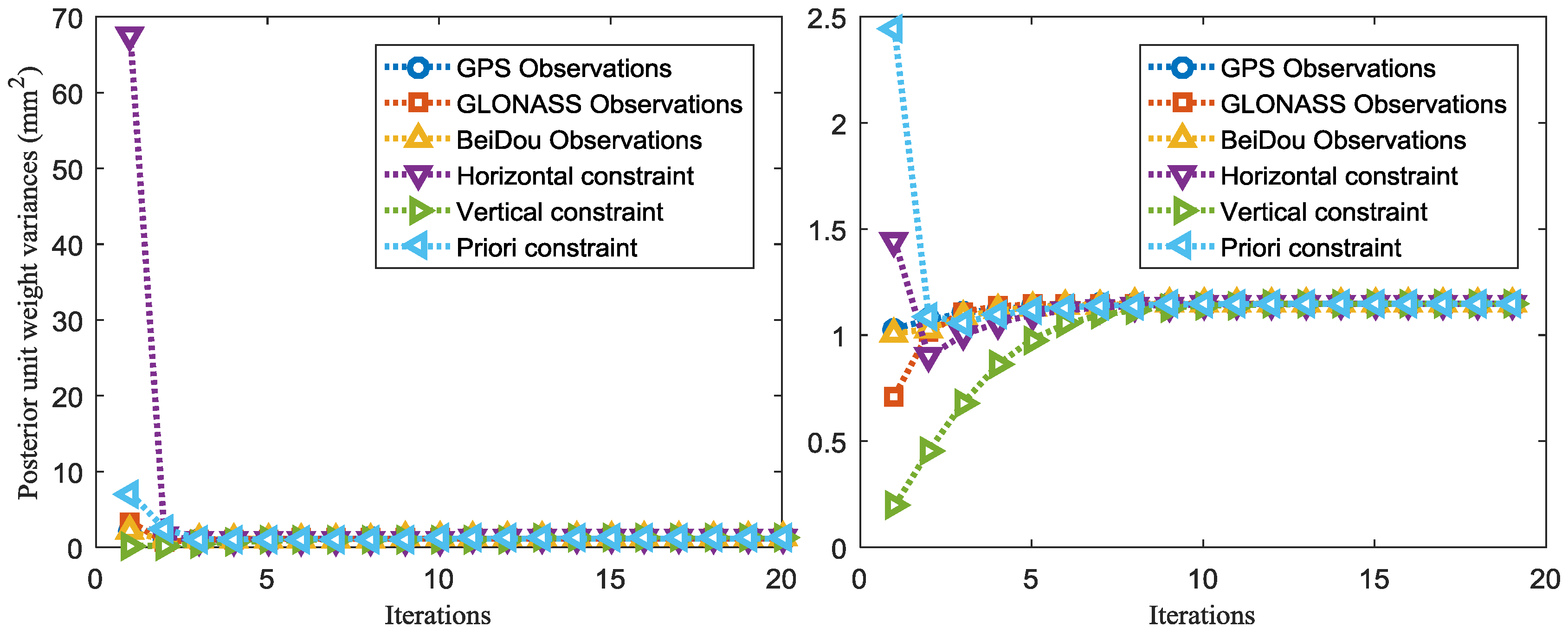
In this section, we first analyzed the change of iterations with the posterior unit weight variance changes as well as the statistics based on the optimal weighting method proposed in Section 2.2. Figure 2 (left) gives the change of posterior unit weight variance for six types of equations with iterations for Scheme 2 at date UTC 12:00 p.m. day of year (Doy) 303, 2015, while the Figure 2 (right) is an enlargement of Figure 2 (left) for the iterations from 2 to 20. As it is presented that the posterior unit weight variances tune to very similar values after two iterations and meet the requirement stated in Section 2.2 after five iterations, five iterations is therefore selected in this resolution. It also can be seen that the posterior unit weight variances of three types of GNSS observations (GPS/GLONASS/BDS) are actually different and converged to the same value gradually, and the value is about 1.15 at UTC 12:00 p.m., Doy 303, 2015 in our experiment after 10 iterations, which manifest the point that the observation equation established using different satellite systems should be regarded as the various input information. Figure 3 shows the relationship between the statistics of improved Bartlett test and iterations over the experimental period of Doy 303 to 317, 2015 with the tomography interval of one hour under the conditions of 10° and 15° elevation angle mask, respectively. It can be clearly seen from Figure 3 that most statistics reach the given criterion after five to seven iterations with the average iterations of 5.5 and 5.7, respectively, which expresses the features of quick convergence of the proposed method mentioned above.

4.2. Internal/External Accuracy Testing

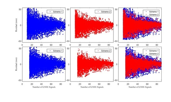
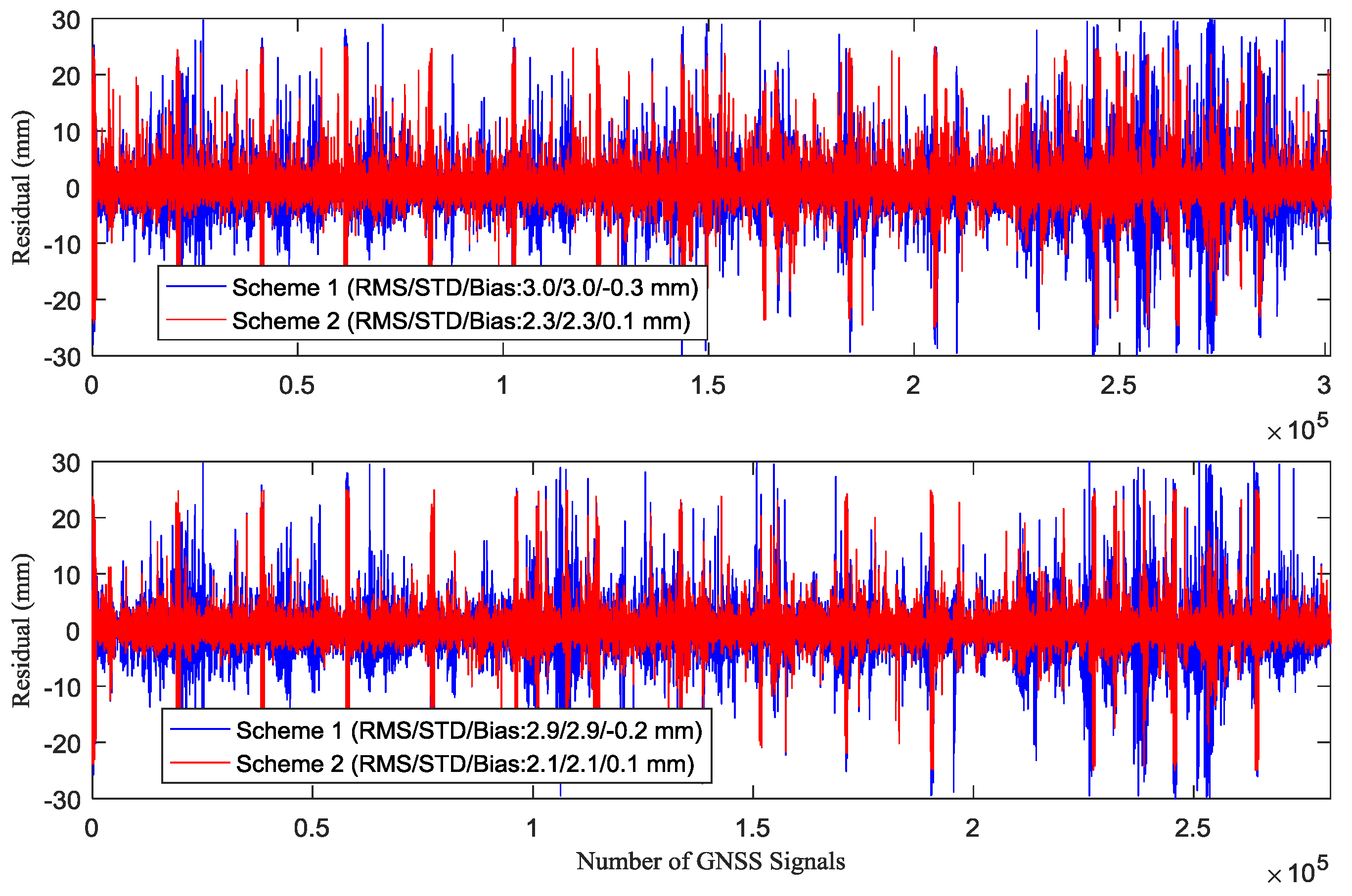
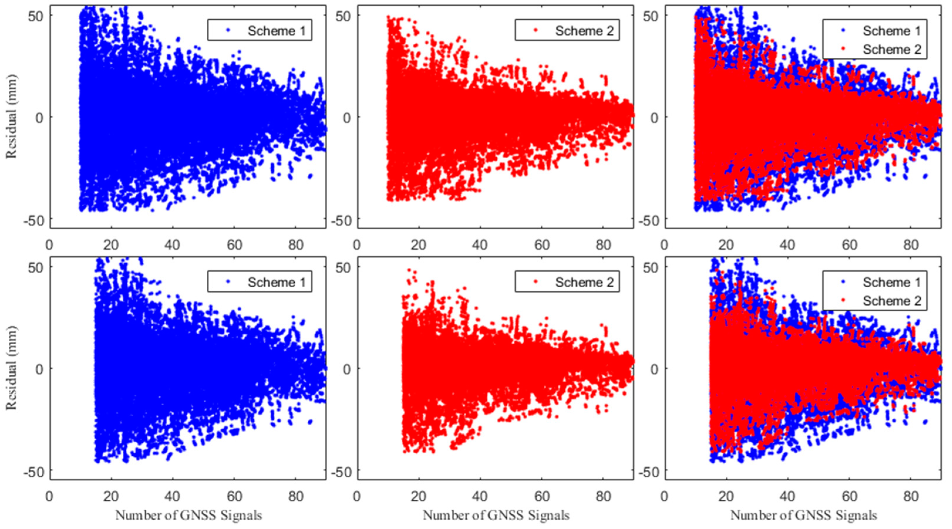
The slant wet delays of six stations (XIUW, BAIY, YONG, QINZ, QINY and KAIY) for the data of Doy 303 to 317, 2015 were used to validate the internal/external accuracy of the proposed method based on the tomographic modeling established in Section 2.1. For the internal accuracy testing, six stations are both used to reconstruct the atmosphere wet refractivity, two elevation angle masks of 10° and 15° were both selected for the two schemes. The residuals of tropospheric delay in the two schemes are shown in Figure 4, where the top and bottom represent the case of 10° and 15° of elevation masks, separately. It is clearly seen that the residual of the proposed method (Scheme 2) is smaller than that of conventional method (Scheme 1) for two cases. The Root Mean Square (RMS) error and the mean bias (Bias) for schemes 1 and 2 are 3.0/−0.3 mm and 2.3/0.1 mm, respectively, under the condition of 10° elevation angle mask while those values are 2.9/−0.2 mm and 2.1/0.1 mm, respectively, under the condition of 15° elevation angle mask. In addition, Figure 5 also gives the change of slant wet delay residuals with elevation angle for two schemes under different elevation angle masks. It is clear that the residuals decreased with ascending elevation angles. The residuals of Scheme 2 (red dots) are obviously smaller than those in Scheme 1 (blue dots) for two cases of 10° and 15° of elevation angle masks.

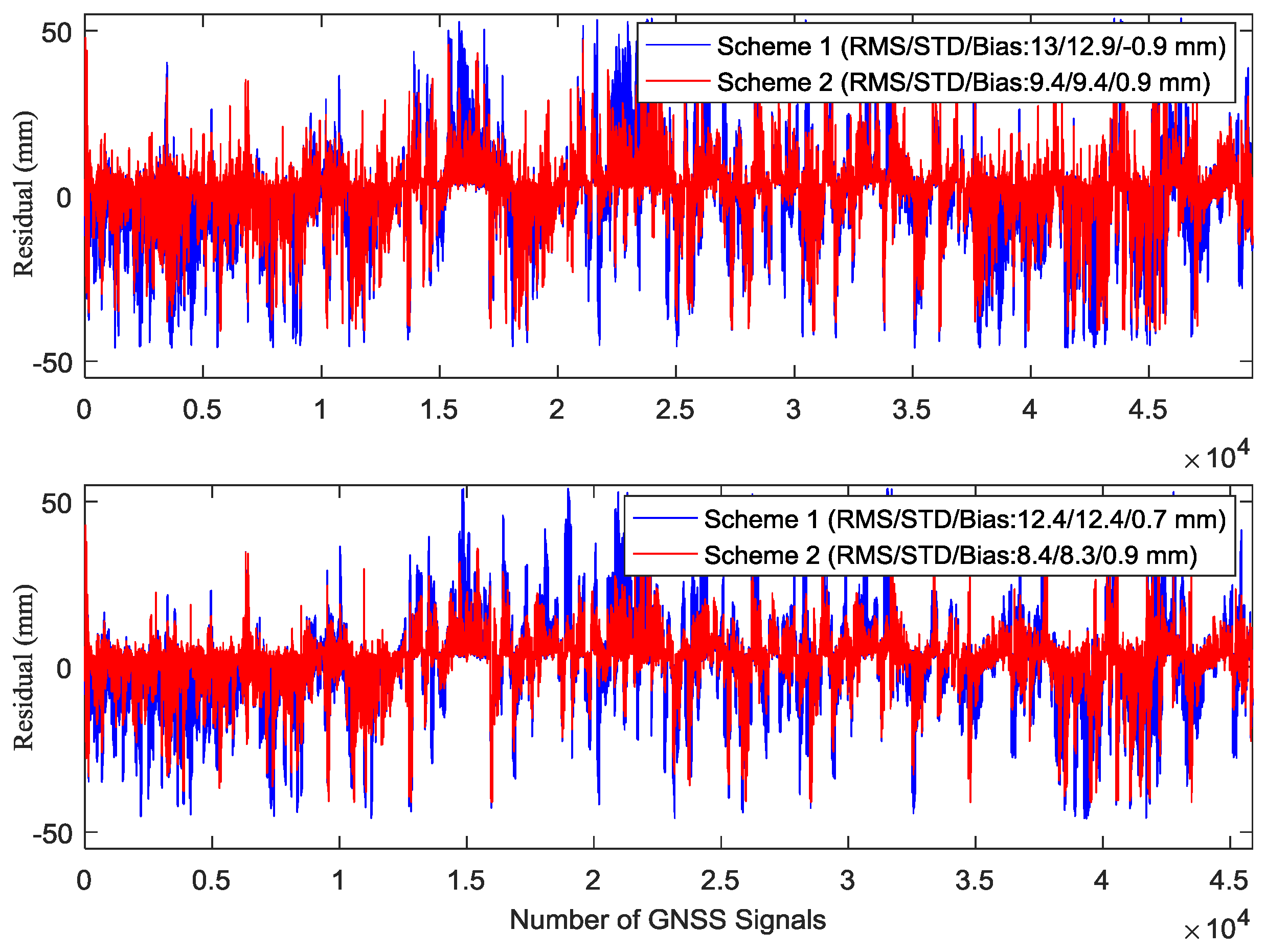
To further assess the proposed method of troposphere tomography using the multi-GNSS observation, another experiment was carried out to validate the external accuracy of the tomography modeling. In this experiment, only five stations (XIUW, YONG, QINZ, QINY and KAIY) were used to reconstruct the wet refractivity for the data of Doy 303 to 317, 2015 with two elevation angle masks of 10° and 15°, respectively. The slant wet delay of BAIY derived from GNSS PPP-estimated is regarded as a reference. Figure 6 shows the residuals of the slant wet delay of the BAIY station for the whole day, where the blue and red lines represent the slant wet delay residuals obtained by Schemes 1 and 2, respectively. It can be clearly seen that the trend of residuals acquired by Scheme 2 fluctuates less wildly than that acquired by Scheme 1. The RMS/Bias for schemes 1 and 2 are 13/−0.9 mm and 9.4/0.9 mm, respectively, under the condition of 10° elevation angle mask while those values are 12.4/0.7 mm and 8.4/0.9 mm, respectively, under the condition of 15° elevation angle mask.

In addition, the trend of slant wet delay residuals of station BAIY with elevation angle were also analyzed and shown in Figure 7. It is clear that the slant wet delay residuals for two schemes decreased with ascending elevation angles. The residuals distribution calculated from Scheme 2 (red dots) obviously shows a smaller change trend than those obtained from Scheme 1 (blue dots) for all ranges of elevation angles.

Table 3. RMS (Root Mean Square) error and Bias of the slant wet delay residuals derived from two schemes in various elevation angle range over the experimental period of Doy 303 to 317, 2015.

Elevation Angle Mask of 10°					Elevation Angle Mask of 15°
Elevation Angle Range (°)	RMS (mm)		Bias (mm)		Elevation Angle Range (°)	RMS (mm)		Bias (mm)
	Scheme		Scheme			Scheme		Scheme
	1	2	1	2		1	2	1	2
10–20	18.9	15.1	−0.5	0.7	15–20	17.7	12.5	0.8	0.8
20–30	14.9	10.0	−0.8	0.9	20–30	15.5	9.8	1.4	1.02
30–40	12.5	9.7	−2.0	−0.6	30–40	12.8	9.4	−0.5	0.6
40–50	10.5	6.7	−0.4	1.5	40–50	10.7	6.5	1.1	1.3
50–60	9.4	6.7	−1.2	0.7	50–60	9.3	6.1	0.3	0.7
60–70	9.0	6.0	−0.4	1.1	60–70	9.1	5.7	0.9	1.3
70–80	8.4	6.0	−0.2	1.3	70–80	8.2	5.4	0.5	1.1
80–90	8.4	5.4	−1.9	0.3	80–90	7.9	4.8	−0.7	0.6

also gives the specific statistical information about the slant wet delays residuals within the elevation angle ranges of 10–20°(15–20°), 20–30°, 30–40°, 40–50°, 50–60°, 60–70°, 70–80°, and 80–90°. Similar conclusions can also be concluded from Table 2 that the RMS error and Bias of slant wet delay residuals acquired by the Scheme 2 is smaller than those by Scheme 1 for different elevation angle masks. The mean RMS error was decreased from 11.4 mm to 7.9 mm and 11.3 mm to 7.1 mm for different cases of elevation angle masks, respectively. In total, the proposed strategy considering the weightings of different observations from multi-GNSS as well as the various constraints can generate a good performance for multi-GNSS troposphere tomography.

4.3. Comparison with Wet Refractivity Derived from Radiosonde Data

It is accepted that the radiosonde data can provide precise atmospheric profile information vertically [40,47,48]. Fortunately, there is a radiosonde station (57816) located in the tomographic area, where the radiosonde balloon is launched twice a day at UTC 12:00 a.m. and 12:00 p.m., respectively. Therefore, such data was also introduced in this paper to validate the accuracy of the tomographic result derived from different schemes. In this experiment, the data of fifteen days from Doy 303 to 317, 2015 was selected for tropospheric tomography and compared with that derived from radiosonde data. Thus, there is a total of thirty sets of data are used and analyzed over the experimental period.

The tomographic wet refractivity value of voxels derived from two schemes were compared with those from radiosonde at the location of the overlapped voxels. The RMS error and Bias of the differences between the radiosonde and different schemes for two epoch (UTC 12:00 a.m. and 12:00 p.m.) of tomography are calculated and showed in Figure 8. It is clearly shown that the values of RMS error and Bias obtained from Scheme 2 are smaller than those from Scheme 1. In addition, the statistical results of wet refractivity between radiosonde and tomography for schemes 1 and 2 was also given and the result reveals that the mean RMS error and Bias of their differences for two schemes are 13.8/8.2 ppm and 3.9/2.8 ppm, respectively.

To further assess the performance of the proposed method considering the weightings of different input information of tomography modeling, the mean wet refractivity profiles at various altitudes derived from two schemes were compared with those from radiosonde over the tested period. In addition, the RMS error of those differences and relative error (RE) are also calculated to analyze the relationship of tomographic modeling error with respect to altitude in Figure 9. It can be clearly seen that the mean wet refractivity profiles of Scheme 2 has a better agreement with that of radiosonde data, especially at the bottom altitudes, compared to that of scheme 1. They also show a smaller value of mean RMS at different altitudes. For the comparison of relative error, the values of Scheme 2 are smaller than those of Scheme 1 below 4 km and shows the opposite case for the above altitudes. From Figure 9 (left), we can see that the water vapor density is mainly focused on the bottom layers, which changes from more than 60 ppm to about 10 ppm at the height of 0–4 km. Therefore, the proposed method in this paper can effectively improve the accuracy of the tomography result, especially at low altitudes. As for the slightly larger relative error above 4 km (Figure 9, right), it is accepted because of the small wet refractivity value in the upper layers, and even a small difference can result in a large relative error.

4.4. Comparison of Final Weightings for Different Observables/Constraints

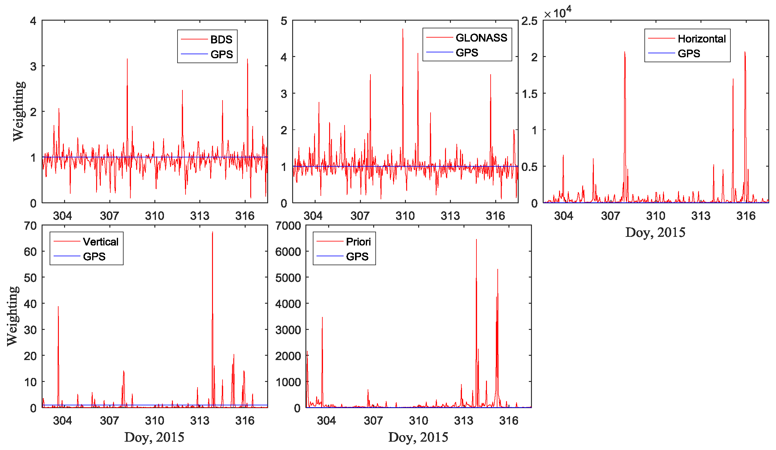
In this section, the change of final weighting for different observables/constraints has been analyzed with the interval of one hour over the period of Doy 303 to 317, 2015 (See Figure 10). It can be seen from Figure 10 that the weighting of different observables/constraints are changed with time, where the weighting of GPS observation is regarded as one in the experiment. For BDS and GLONASS observations, their fluctuatation of final weightings is very small, but the value is different from that with GPS observation, while the values of final weightings for constriaints are very large. The above phenomenon manifested the significance of the proposed method in this paper, which has the ability to tune the weightings of different input information for different epochs.

5. Discussion

The advantage of the proposed method is to obtain the reasonable weightings of tomography observations quickly, but the feasibility remains to be further validated for different regions and weather conditions. With the further development of the GNSS meteorology, the proposed method can also be used for determining the weightings of the different data derived from more multi-GNSS observations. In addition, the weightings of PWV data from Moderate-resolution imaging spectroradiome (MODIS), Constellation Obsering System for Meteorology, Ionosphere, and Climate (COSMIC) and Interferometric Synthetic Aperture Radar (InSAR) used for the troposphere tomography can also be determined based on the method proposed in this manuscript. As for the positioning aspect, [49] proposed five different weighting schemes for the GPS + GLONASS + Galileo + BeiDou combination in real-time PPP, and the result shows, when compared to the GPS-only solution, that the weighted strategy can reduce the formal errors and shorten the convergence time for horizontal and vertical components, respectively. Therefore, the proposed method in this manuscript may also have the potential for determining the accurate weightings of multi-GNSS observations during the PPP processing, but the final result remains to be further verified.

6. Conclusions

In this paper, a tropospheric tomographic method has been proposed, which considers the weightings of multi-GNSS observations as well as that of different constraint information. The data from GPS, GLONASS and BeiDou is used to carry out the experiment, and the improved Bartlett statistics is introduced for the small sample based on the principle of the mean equality in order to determine the final weightings of different input information of tomography modeling. The experimental results using the observed multi-GNSS data show that the posterior unit weight variances of different input information converged to a stable value after three to six iterations for the most epochs. Internal and external accuracy testing are both implemented for two tomography modeling based on the conventional and proposed method under the conditions of 10° and 15° elevation angle masks. For the internal accuracy testing, the RMS error and Bias of Scheme 2 under two kinds of elevation angle masks are both smaller than that of Scheme 1, with the values of 1.6/0.1 mm and 1.3/0.1 mm, respectively. For the external accuracy testing, the same conclusion is also concluded that the slant wet delay residual derived from Scheme 2 has a small discrepancy than those from Scheme 1, with the RMS error and Bias of 5.0/0.9 mm and 4.6/1.1 mm, respectively, under two cases of elevation angle masks.

In addition, the radiosonde data is also introduced to validate the proposed method over the tested period of Doy 303 to 317, 2015, and the statistical results show that the RMS and Bias of the proposed method are both smaller than those of the conventional method, with the value of 9.0/3.1 ppm. By analyzing the relationship of tomographic modeling error with respect to altitudes, we find that the accuracy of tomography result using the proposed method is improved evidently, especially for the height of 0–4 km.

References

- Radon, J. Über die bestimmung von funktionen durch ihre in-te-gral-werte längs gewisser mannigfaltigkeiten. Comput. Tomogr. 1917, 69, 262–277. [Google Scholar]
- Bramlet, R. Reconstruction Tomography in Diagnostic Radiology and Nuclear Medicine. Clin. Nucl. Med. 1978, 3, 245. [Google Scholar]
- Bourjot, L.; Romanowicz, B. Crust and upper mantle tomography in Tibet using surface waves. Geophys. Res. Lett. 1992, 19, 881–884. [Google Scholar]
- Kissling, E.; Ellsworth, W.L.; Eberhart-Phillips, D.; Kradolfer, U. Initial reference models in local earthquake tomography. J. Geophys. Res. Solid Earth 1994, 99, 19635–19646. [Google Scholar]
- Hajj, G.A.; Ibanez-Meier, R.; Kursinski, E.R.; Romans, L.J. Imaging the ionosphere with the Global Positioning System. Int. J. Imaging Syst. Technol. 1994, 5, 174–187. [Google Scholar]
- Braun, J.; Rocken, C.; Meertens, C.; Ware, R. Development of a water vapor tomography system using low cost L1 GPS receivers. In Proceedings of the Ninth ARM Science Team Meeting, US Department of Energy, San Antonio, TX, USA, 22–26 March 1999. [Google Scholar]
- Flores, A.; Ruffini, G.; Rius, A. 4D tropospheric tomography using GPS slant wet delays. Annal. Geophys. 2000, 18, 223–234. [Google Scholar]
- Troller, M. GPS Based Determination of the Integrated and Spatially Distributed Water Vapor in the Troposphere; Swiss Geodetic Commission: Zurich, Switzerland, 2004; Volume 67, p. 70. [Google Scholar]
- Rohm, W.; Bosy, J. Local tomography troposphere model over mountains area. Atmos. Res. 2009, 93, 777–783. [Google Scholar]
- Troller, M.; Geiger, A.; Brockmann, E.; Bettems, J.-M.; Burki, B.; Kahle, H.-G. Tomographic determination of the spatial distribution of water vapor using GPS observations. Adv. Space Res. 2006, 37, 2211–2217. [Google Scholar]
- Skone, S.; Hoyle, V. Troposphere modeling in a regional GPS network. Positioning 2005, 4, 230–239. [Google Scholar]
- Bi, Y.; Mao, J.; Li, C. Preliminary results of 4-D water vapor tomography in the troposphere using GPS. Adv. Atmos. Sci. 2006, 23, 551–560. [Google Scholar]
- Bender, M.; Stosius, R.; Zus, F.; Dick, G.; Wicker, J.; Raabe, A. GNSS water vapour tomography—Expected improvements by combining GPS, GLONASS and Galileo observations. Adv. Space Res. 2011, 47, 886–897. [Google Scholar] [CrossRef]
- Rohm, W. The precision of humidity in GNSS tomography. Atmos. Res. 2012, 107, 69–75. [Google Scholar] [CrossRef]
- Zhang, B.; Fan, Q.; Yao, Y.; Xu, C.; Li, X. An Improved Tomography Approach Based on Adaptive Smoothing and Ground Meteorological Observations. Remote Sens. 2017, 9, 886. [Google Scholar] [CrossRef]
- Bender, M.; Dick, G.; Ge, M.; Deng, Z.; Wicker, J.; Kahle, H.-G.; Raabe, A.; Tetzlaff, G. Development of a GNSS water vapour tomography system using algebraic reconstruction techniques. Adv. Space Res. 2011, 47, 1704–1720. [Google Scholar] [CrossRef]
- Wang, X.; Wang, X.; Dai, Z.; Ke, F.; Cao, Y.; Wang, F.; Song, L. Tropospheric wet refractivity tomography based on the BeiDou satellite system. Adv. Atmos. Sci. 2014, 31, 355–362. [Google Scholar] [CrossRef]
- Benevides, P.; Nico, G.; Catalão, J.; Miranda, P.M. Analysis of Galileo and GPS Integration for GNSS Tomography. IEEE Trans. Geosci. Remote Sens. 2017, 55, 1936–1943. [Google Scholar] [CrossRef]
- Dong, Z.; Jin, S. 3-D Water Vapor Tomography in Wuhan from GPS, BDS and GLONASS Observations. Remote Sens. 2018, 10, 62. [Google Scholar] [CrossRef]
- Guerova, G.; Jones, J.; Dousa, J.; Dick, G.; de Haan, S. Review of the state-of-the-art and future prospects of the ground-based GNSS meteorology in Europe. Atmos. Meas. Tech. 2016, 9, 5385–5406. [Google Scholar] [CrossRef]
- Saastamoinen, J. Contributions to the theory of atmospheric refraction. Bull. Géodésique (1946–1975) 1973, 107, 13–34. [Google Scholar] [CrossRef]
- Rius, A.; Ruffini, G.; Cucurull, L. Improving the vertical resolution of ionospheric tomography with GPS occultations. Geophys. Res. Lett. 1999, 24, 2291–2294. [Google Scholar] [CrossRef]
- Elósegui, P.; Rius, A.; Davis, J.L.; Ruffini, G.; Keihm, S.J.; Burki, B.; Kruse, L.P. An experiment for estimation of the spatial and temporal variations of water vapor using GPS data. Phys. Chem. Earth 1998, 23, 125–130. [Google Scholar] [CrossRef]
- Yao, Y.; Zhao, Q. A novel, optimized approach of voxel division for water vapor tomography. Meteorol. Atmosp. Phys. 2016, 129, 57–70. [Google Scholar] [CrossRef]
- Mikhail, E.; Ackerman, F. Observation and Least Square; A Dun-Donnelley Publisher: New York, NY, USA, 1976; pp. 110–115. [Google Scholar]
- Perera, G.; Carrasco, H.; Díaz, V. Mathematical statistics: On the Hartley-Bartlett test. Int. J. Math. Educ. Sci. Technol. 1996, 27, 553–559. [Google Scholar] [CrossRef]
- Bartlett, M.S. Properties of sufficiency and statistical tests. Proc. R. Soc. Lond. Ser. A Math. Phys. Sci. 1937, 160, 268–282. [Google Scholar] [CrossRef]
- Mahadevan, S. Monte Carlo Simulation; In Mechanical Engineering; Marcel Dekker: New York, NY, USA; Basel, Switzerland, 1997; pp. 123–146. [Google Scholar]
- Zumberge, J.F.; Heflin, M.B.; Jefferson, D.C.; et al. Precise point positioning for the efficient and robust analysis of GPS data from large networks. J. Geophys. Res. Solid Earth 1997, 102, 5005–5017. [Google Scholar] [CrossRef]
- Kouba, J.; Héroux, P. Precise Point Positioning Using IGS Orbit and Clock Products. GPS Solut. 2001, 5, 12–28. [Google Scholar] [CrossRef]
- Cao, X.; Zhang, S.; Kuang, K.; Liu, T.; Gao, K. The Impact of Eclipsing GNSS Satellites on the Precise Point Positioning. Remote Sens. 2018, 10, 94. [Google Scholar] [CrossRef]
- Lou, Y.; Liu, Y.; Shi, C.; Yao, X.; Zheng, F. Precise orbit determination of BeiDou constellation based on BETS and MGEX network. Sci. Rep. 2014, 4, 4692. [Google Scholar] [CrossRef] [PubMed]
- Li, X.; Zhang, X.; Ren, X.; Fritsche, M.; Wicker, J.; Schuh, H. Precise positioning with current multi-constellation global navigation satellite systems: GPS, GLONASS, Galileo and BeiDou. Sci. Rep. 2015, 5, 8328. [Google Scholar] [CrossRef] [PubMed]
- Cai, C.; Gao, Y. Modeling and assessment of combined GPS/GLONASS precise point positioning. GPS Solut. 2013, 17, 223–236. [Google Scholar] [CrossRef]
- Li, P.; Zhang, X.; Guo, F. Ambiguity resolved precise point positioning with GPS and BeiDou. J. Geod. 2017, 91, 25–40. [Google Scholar]
- Guo, F.; Li, X.; Zhang, X.; Wang, J. Assessment of precise orbit and clock products for Galileo, BeiDou, and QZSS from IGS Multi-GNSS Experiment (MGEX). GPS Solut. 2017, 21, 279–290. [Google Scholar] [CrossRef]
- Wanninger, L.; Beer, S. BeiDou satellite-induced code pseudorange variations: Diagnosis and therapy. GPS Solut. 2015, 19, 639–648. [Google Scholar] [CrossRef]
- Niell, A.E. Global mapping functions for the atmosphere delay at radio wavelengths. J. Geophys. Res. Solid Earth 1996, 101, 3227–3246. [Google Scholar] [CrossRef]
- Bevis, M.; Businger, S.; Herring, T.A.; Rocken, C.; Anthes, R.A.; Ware, R.H. GPS meteorology: Remote sensing of atmospheric water vapor using the Global Positioning System. J. Geophys. Res. Atmos. 1992, 97, 15787–15801. [Google Scholar] [CrossRef]
- Niell, A.E.; Coster, A.J.; Solheim, F.S.; Mendes, V.B.; Toor, P.C.; Langley, R.B.; Upham, C.A. Comparison of measurements of atmospheric wet delay by radiosonde, water vapor radiometer, GPS, and VLBI. J. Atmos. Ocean. Technol. 2001, 18, 830–850. [Google Scholar] [CrossRef]
- Boehm, J.; Heinkelmann, R.; Schuh, H. Short note: A global model of pressure and temperature for geodetic applications. J. Geod. 2007, 81, 679–683. [Google Scholar] [CrossRef]
- Lagler, K.; Schindelegger, M.; Böhm, J.; Krásná, H.; Nilsson, T. GPT2: Empirical slant delay model for radio space geodetic techniques. Geophys. Res. Lett. 2013, 40, 1069–1073. [Google Scholar] [CrossRef] [PubMed]
- Hadas, T.; Krypiak Gregorczyk, A.; Hernández Pajares, M.; Kaplon, J.; Paziewski, J.; Wielgosz, P.; Garcia Rigo, A.; Kazmierski, K.; Sosnica, K.; Kwasniak, D.; et al. Impact and Implementation of Higher-Order Ionospheric Effects on Precise GNSS Applications. J. Geophys. Res. Solid Earth 2017, 122, 9420–9436. [Google Scholar] [CrossRef]
- Wu, J.T.; Wu, S.C.; Hajj, G.A.; Bertiger, W.I.; Lichten, S.M. Effects of antenna orientation on GPS carrier phase. In Proceedings of the AAS/AIAA Astrodynamics Conference, San Diego, CA, USA, 19–22 August 1992; pp. 1647–1660. [Google Scholar]
- Petit, G.; Luzum, B. IERS Conventions (2010). Bureau International des Poids et Mesures Sevres (France), 2010. Available online: https://www.iers.org/IERS/EN/Publications/TechnicalNotes/tn36.html (accessed on 1 July 2017).
- Guo, J.; Xu, X.; Zhao, Q.; Liu, J. Precise orbit determination for quad-constellation satellites at Wuhan University: Strategy, result validation, and comparison. J. Geod. 2016, 90, 143–159. [Google Scholar] [CrossRef]
- Liu, Z.; Wong, M.S.; Nichol, J.; Chan, P.W. A multi-sensor study of water vapour from radiosonde, MODIS and AERONET: A case study of Hong Kong. Int. J. Climatol. 2013, 33, 109–120. [Google Scholar] [CrossRef]
- Chen, B.; Liu, Z. Voxel-optimized regional water vapor tomography and comparison with radiosonde and numerical weather model. J. Geod. 2014, 88, 691–703. [Google Scholar] [CrossRef]
- Kazmierski, K.; Hadas, T.; Sośnica, K. Weighting of Multi-GNSS Observations in Real-Time Precise Point Positioning. Remote Sens. 2018, 10, 84. [Google Scholar] [CrossRef]
Figure 1.
Geographic distribution of the selected ground-based GNSS stations in Guiyang and the radiosonde station located in the tomographic area.
Figure 2.
The change of posterior unit weight variances for six types of equations with iteration for Scheme 2 at date UTC 12:00 p.m. Doy 303, UTC 12:00 p.m., 2015.
Figure 3.
The statistics of Bartlett test and iterations under two conditions with elevation angle masks of 10° and 15°, respectively, over the experimental period of Doy 303 to 317, 2015.
Figure 4.
Residuals of the slant wet delay using two schemes with 10° (top) and 15° (bottom) elevation angle mask over the experimental period of Doy 303 to 317, 2015.
Figure 5.
Scatter diagram of the slant wet delay residual using two schemes with 10° (top) and 15° (bottom) elevation angle mask over the experimental period of Doy 303 to 317, 2015.
Figure 6.
Residuals of the slant wet delay for the station of BAIY using two schemes with 10° (top) and 15° (bottom) elevation angle mask over the experimental period of Doy 303 to 317, 2015.
Figure 7.
Scatter diagram of the slant wet delay residual of station BAIY using two schemes with 10° (top) and 15° (bottom) elevation angle masks over the experimental period of Doy 303 to 317, 2015.
Figure 8.
The RMS (Root Mean Square) error and Bias between raidosonde and two schemes for the Doy 303 to 317, 2015.
Figure 9.
Wet refractivity profiles derived from two schemes and radiosonde (left), as well as the RMS and relative error (RE) of their differences (right) at various altitudes over the period of Doy 303 to 317, 2015.
Figure 10.
The change of final weightings for different input information over the period of Doy 303 to 317, 2015, while the weight of GPS observation is regarded as one.