Abstract
Arctic sea ice extent has continued to decline in recent years, and the fractional coverage of multi-year sea ice has decreased significantly during this period. The Beaufort Sea region has been the site of much of the loss of multi-year sea ice, and it continues to play a large role in the extinction of ice during the melt season. We present an analysis of the influence of satellite-derived ice surface temperature, ice thickness, albedo, and downwelling longwave/shortwave radiation as well as latitude and airborne snow depth estimates on the change in sea ice concentration in the Beaufort Sea from 2009 to 2016 using a Lagrangian tracking database. Results from this analysis indicate that parcels that melt during summer in the Beaufort Sea reside at lower latitudes and have lower ice thickness at the beginning of the melt season in most cases. The influence of sea ice thickness and snow depth observed by IceBridge offers less conclusive results, with some years exhibiting higher thicknesses/depths for melted parcels. Parcels that melted along IceBridge tracks do exhibit lower latitudes and ice thicknesses, however, which indicates that earlier melt and breakup of ice may contribute to a greater likelihood of extinction of parcels in the summer.
1. Introduction
Arctic sea ice continues to decline in extent as a result of changes in global climate [1]. This reduction in ice contributes to changes in freshwater balances, the region’s biosphere, energy input at the surface, and the future hardiness of the ice pack against climatic forcing [2]. A reduction of the extent of multi-year sea ice has coincided with this loss of total ice extent, which has led to weakening of the Arctic ice pack [3]. Further study of the major variables influencing these changes in the Arctic is of significant interest to governments, commercial entities, and regional stakeholders [4,5,6].
The Beaufort Sea region of the Arctic in particular has acted as a “sink” for sea ice over the past decade, and it accounts for a significant portion of the total areal loss of sea ice each year [7,8,9,10,11]. The region is the extinction location for many of the multi-year ice floes that advect from the Canadian Archipelago. The loss of multi-year sea ice further weakens the Arctic ice cover against future warming, as older ice floes are typically thicker and stronger than younger floes [12], which can help increase their odds of surviving the summer melt season. Given this region’s relative importance in sea ice loss, it is valuable to explore the factors leading to the survival and/or extinction of ice parcels that reside there.
Through the use of Lagrangian tracking methods, the trajectory of sea ice parcels in the Arctic can be tracked and recorded. These sea ice parcel positions provide a means by which parcels that inhabit a specific region such as the Beaufort Sea can be sorted and analyzed. Further, coincident airborne and satellite data products can be tracked with these parcels over time.
We examine the influence of ice surface temperature (IST), ice thickness, surface albedo, downwelling longwave/shortwave radiation, and snow depth on the change in ice concentration in the Beaufort Sea from 2009 to 2016. Our analysis utilizes a Lagrangian tracking database developed at the University of Colorado that matches sea ice parcel locations with ice surface temperature, albedo, and downwelling longwave and shortwave radiation from satellite-based datasets, and ice thickness from a sea ice model [13]. Furthermore, we compare individual sea ice parcel ice thickness and snow depth as estimated along flight tracks during NASA’s Operation IceBridge [14]. The use of Lagrangian tracked data provides a means by which changes in the health of individual sea ice parcels can be observed over time, with additional initial conditions provided by the airborne observations.
2. Study Area and Data Sources
The Beaufort Sea study region mask utilized in this study is shown in Figure 1. This region contains roughly 6000 12.5 km EASE-Grid cells that formed the study area for this analysis. The landward boundaries of the study region were also conservatively masked in order to prevent the inclusion of parcels that made landfall in this analysis. Sea ice parcel positions were compared against the final Beaufort Sea region mask to determine weeks in which they were present during the study period.
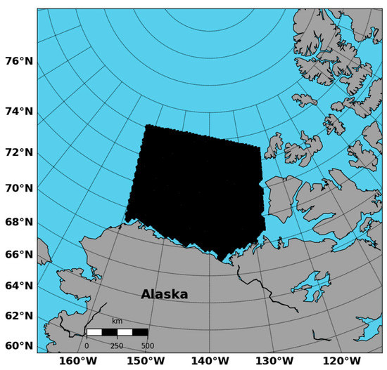
Figure 1.
Beaufort Sea Study Region Shaded in Black.
This analysis utilizes six surface products derived from satellite measurements that are built into a Lagrangian tracking sea ice product [13,15]. Additional airborne data from NASA’s Operation IceBridge Campaigns were also incorporated into the study [14].
2.1. Lagrangian Tracking Product
A database of pan-Arctic Lagrangian tracked ice parcel locations with ancillary sea ice property datasets was utilized for this study [13,15]. The database provides weekly sea ice parcel positions in the Arctic that were used to determine whether particular parcels inhabited the study region. Parcel positions are determined using EASE-Grid sea ice motion vectors [16,17] and ancillary data products from the nearest grid cell to each parcel are provided as part of the dataset [13]. Data are available for 2001–2016 through the Pangaea Data Publisher [15].
2.1.1. APP-x Products
Broadband albedo, downwelling shortwave, and downwelling longwave are obtained from the AVHRR Polar Pathfinder-Extended (APP-x) dataset [18,19]. The data are provided on a 25 km EASE-Grid that is re-gridded to a 12.5 km grid by splitting each 25 km grid cell into four equal-valued cells [13]. Albedo is corrected for clouds, and is derived through the procedures described in [20]. Comparisons of APP-x albedos with SHEBA measurements yielded a bias of −0.05 and an RMSE of 0.1 [19]. Downwelling shortwave and longwave fluxes at the surface are computed using FluxNet: a neural network that was trained to simulate a radiative model [21]. Comparisons of downwelling shortwave radiation with SHEBA campaign measurements obtained a bias of and an RMSE of . Comparisons between downwelling longwave and SHEBA yielded a bias of and an RMSE of [19].
2.1.2. MODIS Terra IST
MODIS ice surface temperatures (IST) are provided through the National Snow and Ice Data Center (NSIDC) on a 4 km EASE-Grid [22], and are re-gridded to fit the 12.5 km EASE-Grid as described in [13]. Comparisons with other IST sources and in-situ measurements have yielded estimated accuracies of 1–3 Kelvin under ideal conditions [23]. The accuracy of the IST data degrades in the presence of clouds and water vapor, which lends to seasonally lower accuracy during the summer [24,25].
2.1.3. SSM/I and SSMI-S Sea Ice Concentration
Sea ice concentrations from SSM/I and SSMI-S are derived through the NASA team algorithm [26], and are available through NSIDC [27]. The data are provided on a 25 km EASE-grid, and are interpolated to fit a 12.5 km EASE-grid as described in [13]. The concentration data are less accurate in the presence of thin ice, melt ponds, and near the ice edge where ocean and atmospheric effects can be mistaken for sea ice. The seasonality of error sources lends to a accuracy during the winter and a accuracy during the summer [27]. Further discussion of the error and performance of the product can be found in [28,29].
2.1.4. PIOMAS Modeled Ice Thickness
The Pan-Arctic Ice-Ocean Modeling and Assimilation System (PIOMAS) provides modeled sea ice thickness derived from a multi-category thickness and enthalpy distribution model [30,31,32]. The model has been compared against submarine and moored ULS and airborne electromagnetic measurements of ice thickness, and has been found to exhibit mean RMS differences near 0.78 m. The model also overestimates thin ice thickness and underestimates thick ice thickness [30]. The product is provided on a stretched generalized orthogonal curvilinear coordinate (GOCC) grid with a displaced north pole that is located in Greenland. The mean resolution of the grid is stated as 4–5, with the greatest resolutions and accuracies being found in the Greenland Sea, Baffin Bay, and the Eastern Canadian Archipelago [32]. The data are re-gridded and interpolated to fit the 12.5 km EASE-Grid as described in [13].
2.2. EASE-Grid Sea Ice Age Data
EASE-Grid sea ice age data based on Lagrangian tracks were obtained from NSIDC in order to investigate the age of parcels advecting through the Beaufort Sea [33]. Sea ice age is based on the NSIDC sea ice motion product [16]. Sea ice motion is estimated by merging calculations from three types of motion vectors: from successive SSM-I passive microwave images, from IABP buoys, and from winds provided by the NCEP/NCAR Reanalysis [16]. Sea ice age is calculated by initially assigning all ice as first-year ice and then, as the model spins up over five simulated years, adding one year of age to each ice parcel that survives the summer melt. The NSIDC sea ice age product is available for 1984–2016, and are provided on a 12.5 km EASE-Grid [33].
2.3. Operation IceBridge Data
Airborne data from spring NASA Operation IceBridge Campaigns were also incorporated into this analysis for years 2009–2016 [14]. The level-4 airborne data were obtained from NSIDC on a 40 m length scale, and are further described in their related documentation page and publication [14,34]. The data include KT-19 infrared pyrometer IST values [35], snow depth estimates retrieved using the University of Kansas’ snow radar [36,37,38], Digital Mapping System (DMS) derived open water concentrations [39], and Airborne Topographic Mapper (ATM) derived thickness estimates [40,41,42].
IceBridge thickness data rely on ATM estimates of freeboard and retrieval of snow depth from radar measurements [14,34]. Freeboard measurements are further refined through the use of DMS measurements to detect leads that are used as surface tie points [34], and final thickness is determined through the use of the hydrostatic balance equation [14]. The mean uncertainty of the thickness data used in this study was 0.82m, and was obtained by averaging the provided uncertainty in each measurement utilized in this analysis. This value is highly variable however, as it depends on several factors that can change in flight [43]. The uncertainty in snow depth estimates is cited as 5.7–5.8 cm [34,44].
3. Methodology
A set of sea ice parcel tracks for 2009–2016 was generated by searching the parcel database files for parcels that resided in the Beaufort Sea study region during any part of each analysis year. Parcels were sorted into two categories containing those that melted during the study year, and those that survived that year’s melt season through the use of a melting threshold of 15% sea ice concentration. Additional checks removed parcels that were considered lost when they coincided with the shore of a land-mask, as these parcels could introduce potentially misleading results into the analysis. The result was a set of weekly observations for parcels that inhabited the Beaufort Sea study area during the years of study. An example of the behavior of the populations in 2009 demonstrates some of the general relationships between the melted and surviving populations present in this data set, such as lower average albedos and ice thickness in the melted parcels (Figure 2).
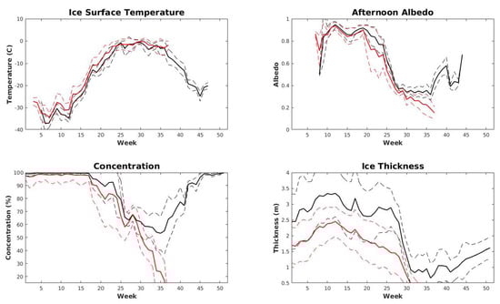
Figure 2.
Example plots of four studied variables for melted (red) and surviving (black) parcels during 2009. Dotted lines indicate one standard deviation away from the main curve.
Weekly averages for values of IST, concentration, thickness, albedo, latitude, and shortwave/ longwave energy input were then computed for both the melted and surviving populations of parcels, with sample sizes shown in Table 1. These values were used to determine Pearson Correlations (measures of the linear relationship) between major variables and change in sea ice concentration. The results of this branch of the analysis are further discussed in Section 4.

Table 1.
Number of melted and surviving parcels analyzed for each year of study.
The Operation IceBridge airborne data were processed by converting the provided latitude and longitude coordinates to EASE-Grid coordinates through the use of the Python Basemap package. Once grid coordinates were obtained, the Operation IceBridge data points were compared against the Beaufort Sea region mask to determine which observations were obtained in the study region. These observations were binned and averaged for each cell with data, and were stored in separate files for use in generating statistics.
The IceBridge flights available in the Beaufort Sea region were sorted by week, and combined to form weekly observation files for each year of study (Table 2). The data used in this analysis included averages of snow depth, concentration, IST, and thickness for each overflown cell along the tracks shown in Figure 3. Parcels with coincident Operation IceBridge data during the weeks of observation were separated into their own distinct melted and surviving populations for the second thrust of this analysis, which is further described in Section 5.
Table 2.
Weeks of IceBridge data for years 2009–2016.
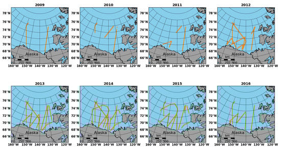
Figure 3.
Operation IceBridge flight track sections utilized for 2009–2016.
4. Results of Analysis of Satellite Data
4.1. Parcel Ages
The percentage of parcels in each age class (1–5+ years) in the Beaufort Sea from 2009–2016 are shown in Figure 4. During years 2009 and 2010, the studied ice parcel population was comprised of approximately 30% old ice (5+ years) that melted. Twenty-five percent of the studied population in 2009 was older ice that survived the transit through the Beaufort Sea, while only 2% of parcels in 2010 were surviving older ice. Years 2011–2016 show a general trend of large losses of first-year sea ice parcels in the Beaufort Sea, with varying losses in the older age classes. In 2013 and 2014, there was an increase in surviving ice aged 5+ years (8% and 11%, respectively), but this increase was followed by an 8% increase in melted older ice during 2015. In 2016, the amount of surviving and melted older ice decreased, with a corresponding rise in melted and surviving young ice (1–2 years). Melted first-year ice made up the largest percent share of ice in all years excepting 2009, in which a large section of multi-year ice had advected into, and melted in, the Beaufort Sea. We observe that in most cases a higher fraction of multi-year ice survives over first-year ice.
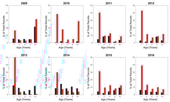
Figure 4.
Percent of population in age categories 1–5+ years for surviving (black) and melted (red) ice parcels in the Beaufort Sea during 2009–2016.
The age of the Arctic ice cover has been declining over recent decades as measured by the EASE-Grid Sea Ice Age Product [3,33]. The extent of ice older than four years of age has decreased from 2.54 million km to 0.13 million km from March 1985 to March 2017 [1]. We observe significant loss of older (5+ years) ice during 2009 and 2010 in the Beaufort Sea, with a large reduction in ice that survived the transit through the region between the two years. While there was a slight recovery in surviving older ice during 2013 and 2014, the following years 2015 and 2016 returned to the general trend of more older ice being extinguished than surviving. The Beaufort Sea has accounted for much of the loss of older ice in previous years [3], and these data suggest that it has continued to play a role in the reduction of older ice in the Arctic due to the advection of older ice from the Canadian Archipelago into the Beaufort Sea.
4.2. Ice Surface Temperatures
Weekly mean ISTs obtained from MODIS data [22] for the melted and surviving parcels in this study are shown in Figure 5. Temperatures for the melted population of sea ice parcels exceeded those of the surviving population for every year of study by an average of 1.8 C. This gap in mean temperatures persisted until the melt season, during which the ice surface is uniformly at its melting temperature. The warmer IST for melted parcels is likely due to the melted population having lower average latitudes, which typically exhibit higher spring temperatures due to greater downwelling shortwave flux and/or advection of warm air masses [45,46].
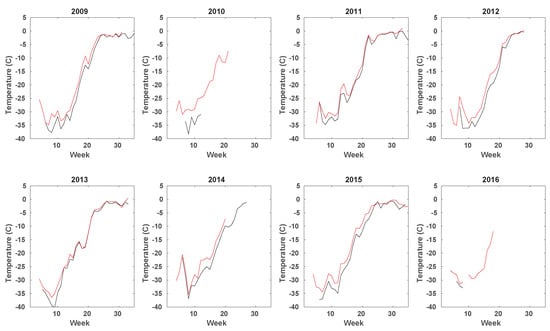
Figure 5.
Ice Surface Temperature trends for melted (red) and surviving (black) parcels during 2009–2016.
4.3. Ice Thickness
Mean weekly sea ice thickness for the melted and surviving parcel populations were obtained from the the Pan-Arctic Ice-Ocean Modeling and Assimilation System (PIOMAS) for years 2009–2016 (Figure 6) [30,31]. Parcels that survived a melt season were 0.5 m thicker on average than their melted counterparts in a given study year. Thicker sea ice parcels should be more likely to survive the melt season due to the larger mass of ice that must be melted to bring the sea ice parcel to the melted threshold of 15%, and their greater ability to resist breakup during collisions. In 2009, we observe an increase in mean thickness for melted parcels near the end of the study period. This is due to a smaller population of thicker parcels surviving at that point in the year.
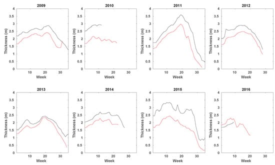
Figure 6.
PIOMAS model ice thickness of melted (red) and surviving (black) sea ice parcels during 2009–2016.
4.4. Mean Latitudes
The mean latitudes of the sea ice parcels, which are shown in Figure 7, had a strong influence on the probability of survival in all years of study. Surviving parcels were typically 2–3 higher in latitude than melted parcels prior to the onset of melt. As the melt season progressed, the mean latitude of melted parcels progresses northward with the retreating ice edge, but this is a typical seasonal pattern of ice retreat.
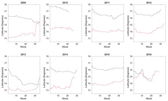
Figure 7.
Mean latitudes of sea ice parcel populations during 2009–2016. Melted parcels are shown in red, surviving parcels are shown in black.
4.5. Downwelling Radiative Fluxes
Downwelling shortwave and longwave radiative fluxes were obtained from the APP-x dataset [19]. Mean downwelling shortwave radiative fluxes for melted and surviving parcels were very similar for all years in the study period (Figure 8). The melted population typically received 10–15 W/m more downwelling shortwave flux during the first part of the year, but after Week 20 the surviving population received up to 20 W/m more downwelling flux. Mean downwelling longwave radiative fluxes were also very similar for both the surviving and melted parcels, with periods of up to 10 W/m greater downwelling flux for the melted parcel population (Figure 9). The relationship of greater downwelling longwave flux for melted parcels typically held during later parts of the study years.
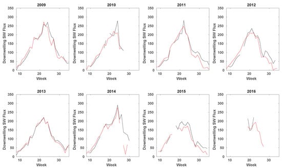
Figure 8.
Mean downwelling shortwave radiation in W/m for surviving (black) and melted (red) parcels during 2009–2016.
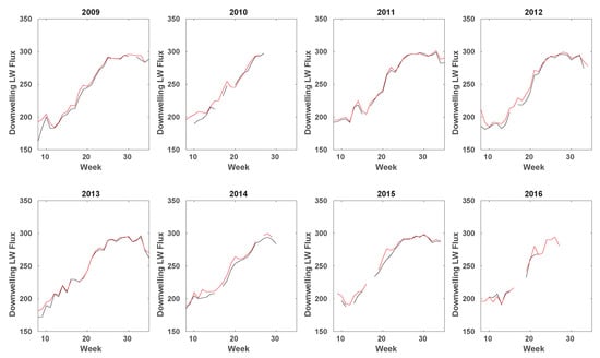
Figure 9.
Mean downwelling longwave radiation in W/m for surviving (black) and melted (red) parcels during 2009–2016.
4.6. Surface Albedos
The mean APP-x [19] albedos of the melted and surviving parcels in this study are shown in Figure 10. The albedos in the melted populations were lower than the surviving parcel population means, which led to greater energy input for equal radiative forcing at the surface in the melted population. The mean difference was typically 0.1, which represents a significant difference in available shortwave radiation during the melt season.
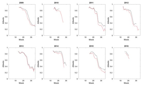
Figure 10.
Mean albedo for melted (red) and surviving (black) parcels during 2009–2016.
4.7. Pearson Correlations between Major Variables and Concentration Change
Pearson correlations were calculated to explore the linear relationship between the major thermodynamic variables discussed above, and the change in sea ice parcel concentration obtained from SSMI/SSMI-S [27] for the overall sample population in each year (Table 3). Due to the use of total change in parcel concentration as the variable to compare against, positive correlations imply that an increase in the variable will lead to an increase in melt rate, while negative correlations imply that an increase in the variable will lead to a decrease in melt rate.
Table 3.
Pearson correlations between studied variables and total change in concentration for 2009–2016. Values with p > 0.05 are shown in red.
5. Results for Parcels with Coincident Operation IceBridge Data
The Operation IceBridge data analyzed in this study were comprised of twenty-six separate flights over the Beaufort Sea study region during the analysis period. Files containing coincident data for a given week were combined to form weekly observation files for use in computing mean surface conditions for each year (Table 4). The year 2009 featured one week of data, while the years 2010–2016 each had two weeks of data to use as a point of comparison (Table 2). These data provided initial values for parcels prior to the onset of melt.
Table 4.
Mean Operation IceBridge and satellite derived spring surface conditions of melted (red) and surviving (black) ice parcels.
Ice surface temperature measurements from Operation IceBridge were available in the region of study for all observation years except 2009, 2011, and 2016 [35]. These data showed an average IST difference between melting and surviving populations of 5.8 C. The relationship of higher average temperatures for melted parcels as compared to surviving parcels held for all years in this analysis. This relationship is also present in the satellite IST means for this subset of parcels. These results match those described in the previous section, where the population of melted parcels endured higher surface temperatures than the surviving population during the spring. IST can change quickly from day to day however, so these results are limited due to their sparse sampling.
Snow depth was also considered in this analysis, as its higher albedo and negative heat flux contribution can help prevent the loss of an ice parcel by delaying melt [47]. Snow depths were greater in the surviving sea ice parcel population for all years except 2010 and 2016. Outside of years 2010 and 2016, the surviving parcels possessed an average of 5 cm greater snow depths than their melted counterparts.
Results from Operation IceBridge ice thickness estimates and PIOMAS model thicknesses yield contrasting results. In the IceBridge data, the melted parcels had an average of 27 cm greater mean ice thickness than surviving parcels in 2009, while melted parcels in 2010 and 2012 were an average of 4.5 cm thicker than surviving parcels. In 2014, the average thickness of surviving parcels exceeded that of melted parcels by 48 cm, and surviving parcels were an average of 10.5 cm thicker than melted parcels in 2015 and 2016. Coincident PIOMAS thickness data for these parcels indicate that surviving parcels were thicker in every year by an average of 30 cm.
IceBridge concentration data for all years in which they were available indicate that sea ice parcels in both populations were near 100% sea ice concentration. SSMI sea ice concentrations along the flight tracks were also at or near 100%. While lower ice concentrations are possible in some regions during the spring, there weren’t parcels lower then 100% present in the IceBridge estimates used in this study.
6. Discussion
For the satellite data studied from 2009–2016, we observe that albedo exhibited the strongest negative Pearson correlation with change in ice concentration. This is likely a result of the ice albedo feedback [48,49]. The downwelling longwave radiative flux had the highest positive Pearson correlation with change in ice concentration. These results agree well with other studies that have found that greater downwelling longwave radiation in the spring, and other linked processes, contribute to earlier melt onset and lower end of season ice extent [50,51,52]. We note that downwelling shortwave flux correlated negatively with change in ice concentration, but this is likely due to the observed seasonal decline in downwelling shortwave radiation (Figure 8) while melt continues at the end of the melt season [46]. Other studies have suggested that longwave radiation anomalies have a greater impact on melt onset, while shortwave radiation anomalies act as an amplifying feedback once melt has started [51].
We observe that melted out parcels are located at lower latitudes and are thinner than surviving ice parcels prior to the onset of melt. These parcels are more likely to break up due to their lower ice thickness, which further contributes to their extinction due to increased lateral melt from the surrounding ocean [53]. We also observe that first year ice comprised the majority of melted ice in all years except 2009. The predominance of younger ice in the melted population is linked to the thickness of the ice, as older parcels are generally thicker than younger ones [12].
For the subset of parcels that had IceBridge data available during 2009–2016, we observe that spring snow depth may influence the survival of ice parcels in the Beaufort Sea, but these results are inconclusive. Sea ice parcels that survived a summer melt season had an average of 5 cm of additional snow cover when compared against those that did not survive the melt season. Snow depth data from two of the study years exhibited greater average snow depth for the melted parcel population however, so there isn’t conclusive evidence that snow depth directly contributes to survival. The potential importance of snow is linked with our previous discussion of albedo, as snow on the sea ice surface helps to delay melt onset by protecting the ice from further energy input through its higher albedo [47,54]. This is limited to the summer melt season however, as snow can dampen sea ice growth during the fall and winter seasons [55].
We observe that IceBridge parcels had mixed results for parcel ice thickness throughout the study period, with half of the years exhibiting greater mean ice thickness in the melted population. The mean latitude of melted parcels was lower than that of the surviving parcels, which may have contributed to the extinction of thicker parcels during years in which mean thicknesses in the melted population exceeded those of the survivors. PIOMAS model data for these parcels show that surviving parcels were thicker than melted parcels in all study years. The reported uncertainties for PIOMAS model thicknesses and IceBridge thickness estimates were similar for this study. The difference between the IceBridge and PIOMAS results may be a result of the smaller 40 m footprint of IceBridge observations as compared to the 12.5 km PIOMAS values. This difference in sampling size causes IceBridge tracks to report thicknesses for a much smaller region of ice as compared to the PIOMAS averages over entire EASE-Grid cells, which could lead to the mixed results that we observe for IceBridge thicknesses.
We note that, while this study has demonstrated the use of Lagrangian tracks to study sea ice parcel histories in a region of interest, its results are limited by several key factors. This analysis excludes ocean surface temperatures under the ice, which are an important factor during the melt season [56]. Dynamic variables such as surface winds and their impact on the deformation and further breakup of sea ice were also not considered. In addition, the variables considered in this work, such as snow cover and albedo, are not independent [57], and there are other factors that influence the extinction of ice in the Beaufort Sea. The results from this study do suggest that albedo, initial latitude, and thickness are the strongest predictors of ice survival for the variables studied. Results for snow are less conclusive, but snow on sea ice is an ongoing area of study [47,55,58,59]. Future sources of snow data should help to further clarify its influence on the survival of sea ice parcels in the Beaufort Sea.
7. Conclusions
Major variables influencing the survival of sea ice in the Beaufort Sea during 2009–2016 have been considered through the combined use of a Lagrangian tracking database of sea ice parcels and coincident Operation IceBridge airborne observations. The parcels have been sorted into melted and survived categories, and their weekly average values of IST, albedo, latitude, and downwelling longwave/shortwave radiation have been compared against weekly concentration change. Additional average values of snow depth, thickness, IST, and concentrations estimates from NASA’s Operation IceBridge flights during the spring have also been compared.
The results of this study indicate that albedo appears to linearly correlate most with percent change in sea ice concentration, and thus survival, of sea ice parcels in the Beaufort Sea. Parcels that survived the summer melt had consistently higher initial albedos than those that melted. The Pearson correlation between albedo and change in concentration was found to have the strongest negative correlation of the variables studied, while downwelling longwave radiative flux was most positively correlated with change in concentration.
We also observe that melted parcels were located at lower latitudes earlier in the year, and were thinner than their surviving counterparts. This led to earlier reduction in sea ice concentration that likely contributed to the extinction of these sea ice parcels. Melted parcels with coincident IceBridge data were located at lower latitudes than surviving parcels, but there were several years in which melted parcels had greater mean ice thickness. This is in contrast with PIOMAS model data along the flight tracks, which exhibit greater mean thicknesses for surviving parcels in all years. We conclude that the disagreement between the IceBridge and PIOMAS data is likely due to the limited footprint of the IceBridge observations, which can misrepresent the overall thickness of a 12.5 km EASE-Grid cell due to sampling limitations. Results from IceBridge snow radar estimates are inconclusive, as melted and surviving parcels did not exclusively exhibit higher or lower depths in all cases.
Additional research with more sources of snow data throughout the spring are warranted. The inclusion of more thermodynamic and dynamic data sources to this analysis would also help provide context for possible breakup of ice and input of additional energy at the surface and from the underlying ocean. The use of statistical learning techniques on the Lagrangian tracking data utilized in this study may also be of future interest for addressing these relationships.
Acknowledgments
The authors would like to acknowledge support from NASA Grant #NNX16AQ41G for the work in this publication. The authors also acknowledge contributions from three anonymous reviewers of this publication, whose comments greatly improved the quality of this manuscript.
Author Contributions
Matthew Tooth created codes to perform the airborne/satellite data comparisons. Mark Tschudi and Matthew Tooth contributed to the analysis of the resulting data. Matthew Tooth and Mark Tschudi both contributed to the production and editing of this manuscript.
Conflicts of Interest
The authors declare no conflict of interest.
Abbreviations
The following abbreviations are used in this manuscript:
| APP-x | Extended AVHRR Polar Pathfinder |
| ATM | Airborne Topographic Mapper |
| DMS | Digital Mapping Sensor |
| EASE | Equal-Area Scalable Earth |
| GOCC | Generalized Orthogonal Curvilinear Coordinate |
| IST | Ice surface temperature |
| LW | Longwave Radiation |
| MODIS | Moderate Resolution Imaging Spectroradiometer |
| NSIDC | National Snow and Ice Data Center |
| PIOMAS | Pan-Arctic Ice Ocean Modeling and Assimilation System |
| SSM/I | Special Sensor Microwave Imager |
| SSMIS | Special Sensor Microwave Imager/Sounder |
| SW | Shortwave Radiation |
References
- Richter-Menge, J.; Overland, J.E.; Mathis, J.T.; Osborne, E. Arctic Report Card 2017. Available online: http://www.arctic.noaa.gov/Report-Card (accessed on 8 January 2018).
- Stroeve, J.C.; Markus, T.; Boisvert, L.; Miller, J.; Barrett, A. Changes in Arctic Melt Season and Implications for Sea Ice Loss. Geophys. Res. Lett. 2014, 41, 1216–1225. [Google Scholar] [CrossRef]
- Maslanik, J.; Stroeve, J.; Fowler, C.; Emery, W. Distribution and Trends in Arctic Sea Ice Age Through Spring 2011. Geophys. Res. Lett. 2011, 38, L13502. [Google Scholar] [CrossRef]
- Ebinger, C.K.; Zambetakis, E. The Geopolitics of Arctic Melt. Int. Aff. 2009, 85, 1215–1232. [Google Scholar] [CrossRef]
- Melia, N.; Haines, K.; Hawkins, E. Sea Ice Decline and 21st Century Trans-Arctic Shipping Routes. Geophys. Res. Lett. 2016, 43, 9720–9728. [Google Scholar] [CrossRef]
- Emmerson, C.; Lahn, G. Lloyd’s Arctic Opening: Opportunity and Risk in the High North. Available online: https://www.lloyds.com/~/media/files/news%20and%20insight/360%20risk%20insight/arctic_risk_report_webview.pdf (accessed on 8 January 2018).
- Stroeve, J.; Serreze, M.; Holland, M.; Kay, J.; Maslanik, J.; Barrett, A. The Arctic’s Rapidly Shrinking Sea Ice Cover: A Research Synthesis. Clim. Chang. 2012, 110, 1005–1027. [Google Scholar] [CrossRef]
- Proshutinsky, A.; Dukhovskoy, D.; Timmermans, M.L.; Krishfield, R.; Bamber, J. Arctic Circulation Regimes. Philos. Trans. R. Soc. A Math. Phys. Eng. Sci. 2015. [Google Scholar] [CrossRef] [PubMed]
- Krishfield, R.A.; Proshutinsky, A.; Tateyama, K.; Williams, W.J.; Carmack, E.C.; McLaughlin, F.A.; Timmermans, M.L. Deterioration of Perennial Sea Ice in the Beaufort Gyre from 2003 to 2012 and its Impact on the Oceanic Freshwater Cycle. J. Geophys. Res. Oceans 2014, 119, 1271–1305. [Google Scholar] [CrossRef]
- Howell, S.; Brady, M.; Derksen, C.; Kelly, R. Recent Changes in Sea Ice Area Flux Through the Beaufort Sea during the Summer. J. Geophys. Res. Oceans 2016, 121, 2569–2672. [Google Scholar] [CrossRef]
- Steele, M.; Dickinson, S.; Zhang, J.; Lindsay, R. Seasonal Ice Loss in the Beaufort Sea: Toward Synchrony and Prediction. J. Geophys. Res. Oceans 2015, 120, 1118–1132. [Google Scholar] [CrossRef]
- Tschudi, M.; Stroeve, J.; Stewart, S. Relating the Age of Arctic Sea Ice to its Thickness, as Measured during NASA’s ICESat and IceBridge Campaigns. Remote Sens. 2016, 8, 457. [Google Scholar] [CrossRef]
- Tooth, M.; Tschudi, M. A Database of Weekly Sea Ice Parcel Tracks Derived from Lagrangian Motion Data with Ancillary Data Products. Data 2017, 2, 25. [Google Scholar] [CrossRef]
- Kurtz, N.; Studinger, M.S.; Harbeck, J.; Onana, V.; Yi, D. IceBridge L4 Sea Ice Freeboard, Snow Depth, and Thickness; NASA DAAC at the National Snow and Ice Data Center: Boulder, CO, USA, 2015.
- Tooth, M.; Tschudi, M. EASE-Grid Sea Ice Parcel Tracks with Ancillary Satellite Data Products from 2001 to 2016. Pangaea Data Publ. Earth Data Sci. 2017. [Google Scholar] [CrossRef]
- Tschudi, M.; Fowler, C.; Maslanik, J.; Stewart, J.S.; Meier, W. Polar Pathfinder Daily 25 km EASE-Grid Sea Ice Motion Vectors; NASA DAAC at the National Snow and Ice Data Center: Boulder, CO, USA, 2016.
- Tschudi, M.; Fowler, C.; Maslanik, J. Tracking the Movement and Changing Surface Characteristics of Arctic Sea Ice. IEEE J. Sel. Top. Appl. Earth Obs. Remote Sens. 2010, 3, 536–540. [Google Scholar] [CrossRef]
- Key, J.; Wang, X.; Liu, Y. NOAA Climate Data Record of AVHRR Polar Pathfinder Extended (APP-X), Version 1, Revision 1; NOAA National Climatic Data Center: Asheville, NC, USA, 2014.
- Key, J.; Wang, X.; Liu, Y.; Dworak, R.; Letterly, A. The AVHRR Polar Pathfinder Climate Data Records. Remote Sens. 2016, 8, 167. [Google Scholar] [CrossRef]
- Key, J.; Wang, X.; Stroeve, J.; Fowler, C. Estimating the Cloudy-Sky Albedo of Sea Ice and Snow from Space. J. Geophys. Res. Atmos. 2001, 106, 12489–12497. [Google Scholar] [CrossRef]
- Key, J.; Schweiger, A. Tools for Atmospheric Radiative Transfer: Streamer and FluxNet. Comput. Geosci. 1998, 24, 443–451. [Google Scholar] [CrossRef]
- Hall, D.K.; Riggs, G.A. MODIS/Terra Sea Ice Extent and IST Daily L3 Global 4 km EASE-Grid Day, Version 6; NASA DAAC at the National Snow and Ice Data Center: Boulder, CO, USA, 2015.
- Hall, D.K.; Nghiem, S.; Rigor, I.; Miller, J. Uncertainties of Temperature Measurements on Snow-Covered Land and Sea Ice from In-Situ and MODIS Data during BROMEX. J. Appl. Meteorol. Climatol. 2015, 54, 966–978. [Google Scholar] [CrossRef]
- Scambos, T.A.; Haran, T.M.; Massom, R. Validation of AVHRR and MODIS Ice Surface Temperature Products Using In-Situ Radiometers. Ann. Glaciol. 2006, 44, 345–351. [Google Scholar] [CrossRef]
- Shuman, C.A.; Hall, D.K.; DiGirolamo, N.; Mefford, T.; Schnaubelt, M. Comparison of Near-Surface Air Temperatures and MODIS Ice Surface Temperatures at Summit, Greenland (2008–2013). J. Appl. Meteorol. Climatol. 2014, 53, 2171–2180. [Google Scholar] [CrossRef]
- Cavalieri, D. NASA Sea Ice Validation Program for the DMSP SMM/I: Final Report; NASA Technical Memorandum 104559; National Aeronautics and Space Administration: Washington, DC, USA, 1992.
- Cavalieri, D.; Parkinson, C.; Gloersen, P.; Zwally, H.J. Sea Ice Concentrations From Nimbus-7 SMMR and DMSP SSM/I-SSMIS Passive Microwave Data; NASA DAAC at the National Snow and Ice Data Center: Boulder, CO, USA, 1996.
- Ivanova, N.; Pedersen, L.T.; Tonboe, R.T.; Kern, S.; Heygster, G.; Lavergne, T.; Sørensen, A.; Saldo, R.; Dybkjær, G.; Brucker, L.; et al. Inter-Comparison and Evaluation of Sea Ice Algorithms: Towards Further Identification of Challenges and Optimal Approach Using Passive Microwave Observations. Cryosphere 2015, 9, 1797–1817. [Google Scholar] [CrossRef]
- Andersen, S.; Tonboe, R.; Kaleschke, L.; Heygster, G.; Pedersen, L.T. Intercomparison of Passive Microwave Sea Ice Concentration Retrievals over the High-Concentration Arctic Sea Ice. J. Geophys. Res. Oceans 2007, 112, C08004. [Google Scholar] [CrossRef]
- Schweiger, A.; Lindsay, R.; Zhang, J.; Steele, M.; Stern, H. Uncertainty in Modeled Arctic Sea Ice Volume. J. Geophys. Res. Oceans 2011. [Google Scholar] [CrossRef]
- Wang, X.; Key, J.; Kwok, R.; Zhang, J. Comparison of Arctic Sea Ice Thickness from Satellites, Aircraft, and PIOMAS Data. Remote Sens. 2016, 8, 713. [Google Scholar] [CrossRef]
- Zhang, J.; Rothrock, D.A. Modeling Global Sea Ice with a Thickness and Enthalpy Distribution Model in Generalized Curvilinear Coordinates. Mon. Weather Rev. 2003, 131, 845–861. [Google Scholar] [CrossRef]
- Tschudi, M.; Fowler, C.; Maslanik, J.; Stewart, J.S.; Meier, W. EASE-Grid Sea Ice Age, Version 3; NASA DAAC at the National Snow and Ice Data Center: Boulder, CO, USA, 2016. [CrossRef]
- Kurtz, N.T.; Farrell, S.L.; Studinger, M.; Galin, N.; Harbeck, J.P.; Lindsay, R.; Onana, V.D.; Panzer, B.; Sonntag, J.G. Sea Ice Thickness, Freeboard, and Snow Depth Products from Operation IceBridge Airborne Data. Cryosphere 2013, 7, 1035–1056. [Google Scholar] [CrossRef]
- Krabill, W.B.; Buzay, E. IceBridge KT19 IR Surface Temperature, Version 1; NASA DAAC at the National Snow and Ice Data Center: Boulder, CO, USA, 2012.
- Kwok, R.; Panzer, B.; Leuschen, C.; Pang, S.; Markus, T.; Holt, B.; Gogineni, S. Airborne Surveys of Snow Depth over Arctic Sea Ice. J. Geophys. Res. Oceans 2011, 116, C11018. [Google Scholar] [CrossRef]
- Rodriguez-Morales, F.; Gogineni, S.; Leuschen, C.J.; Paden, J.D.; Li, J.; Lewis, C.C.; Panzer, B.; Gomez-Garcia, D.; Patel, A.; Byers, K.; et al. Advanced Multifrequency Radar Instrumentation for Polar Research. IEEE Trans. Geosci. Remote Sens. 2014, 52, 2824–2842. [Google Scholar] [CrossRef]
- Kanagaratnam, P.; Markus, T.; Lytle, V.; Heavey, B.; Jansen, P.; Prescott, G.; Gogineni, S.P. Ultrawideband Radar Measurements of Thickness of Snow Over Sea Ice. IEEE Trans. Geosci. Remote Sens. 2007, 45, 2715–2724. [Google Scholar] [CrossRef]
- Dominguez, R. IceBridge DMS L1B Geolocated and Orthorectified Images, Version 1; NASA DAAC at the National Snow and Ice Data Center: Boulder, CO, USA, 2010.
- Brunt, K.M.; Hawley, R.; Lutz, E.; Studinger, M.; Sonntag, J.; Hofton, M.; Andrews, L.; Neumann, T. Assessment of NASA Airborne Laser Altimetry Data Using Ground-Based GPS Data Near Summit Station, Greenland. Cryosphere 2017, 11, 681–692. [Google Scholar] [CrossRef]
- Kwok, R.; Cunningham, G.F.; Manizade, S.S.; Krabill, W.B. Arctic Sea Ice Freeboard from IceBridge Acquisitions in 2009: Estimates and Comparisons with ICESat. J. Geophys. Res. Oceans 2012, 117, C02018. [Google Scholar] [CrossRef]
- Yi, D.; Harbeck, J.; Manizade, S.; Kurtz, N.; Studinger, M.; Hoft, M. Arctic Sea Ice Freeboard Retrieval with Waveform Characteristics for NASA’s Airborne Topographic Mapper (ATM) and Land, Vegetation, and Ice Sensor (LVIS). IEEE Trans. Geosci. Remote Sens. 2015, 53, 1403–1410. [Google Scholar] [CrossRef]
- Kurtz, N.; Harbeck, J. Operation IceBridge Sea Ice Freeboard, Snow Depth, and Thickness Data Products Manual, Version 2 Processing. NSIDC, 2015. Available online: https://nsidc.org/sites/nsidc.org/files/files/data/icebridge/IDCSI4-icebridge-products-manual-Version2-June-2015.pdf (accessed on 10 January 2018).
- Farrell, S.; Kurtz, N.; Connor, L.; Elder, B.; Leuschen, C.; Markus, T.; McAdoo, D.; Panzer, B.; Richter-Menge, J.; Sontaag, J. A First Assessment of IceBridge Snow and Ice Thickness Data Over Arctic Sea Ice. IEEE Trans. Geosci. Remote Sens. 2012, 50. [Google Scholar] [CrossRef]
- Rigor, I.; Colony, R.; Martin, S. Variations in Surface Air Temperature Observations in the Arctic, 1979–1997. J. Clim. 2000, 13, 896–914. [Google Scholar] [CrossRef]
- Serreze, M.; Barry, R. The Arctic Climate System, 2nd ed.; Cambridge University Press: New York, NY, USA, 2014; pp. 146–147. [Google Scholar]
- Perovich, D.; Polashenski, C.; Arntsen, A.; Stwertka, C. Anatomy of a Late Spring Snowfall on Sea Ice. Geophys. Res. Lett. 2017, 44, 2802–2809. [Google Scholar] [CrossRef]
- Curry, J.A.; Schramm, J.L. Sea Ice-Albedo Climate Feedback Mechanism. J. Clim. 1995, 8, 240–247. [Google Scholar] [CrossRef]
- Perovich, D.; Light, B.; Eicken, H.; Jones, K.; Runciman, K.; Nghiem, S. Increasing Solar Heating of the Arctic Ocean and Adjacent Seas, 1979-2005: Attribution and Role in the Ice-Albedo Feedback. Geophys. Res. Lett. 2007, 34, L19505. [Google Scholar] [CrossRef]
- Mortin, J.; Svensson, G.; Graversen, R.; Kapsch, M.L.; Stroeve, J.; Boisvert, L. Melt Onset over Arctic Sea Ice Controlled by Atmospheric Moisture Transport. Geophys. Res. Lett. 2016, 43, 6636–6642. [Google Scholar] [CrossRef]
- Kapsch, M.; Graversen, R.; Tjernstrom, M. Springtime Atmospheric Energy Transport and the Control of Arctic Summer Sea-Ice Extent. Nat. Clim. Chang. 2013, 3, 744–748. [Google Scholar] [CrossRef]
- Kapsch, M.; Graversen, R.; Tjernstrom, M.; Bintanja, R. The Effect of Downwelling Longwave and Shortwave Radiation on Arctic Summer Sea Ice. J. Clim. 2016, 29, 1143–1159. [Google Scholar] [CrossRef]
- Tsamados, M.; Feltham, D.; Petty, A.; Schroeder, D.; Flocco, D. Processes Controlling Surface, Bottom, and Lateral Melt of Arctic Sea Ice in a State of the Art Sea Ice Model. Philos. Trans. R. Soc. A Math. Phys. Eng. Sci. 2015. [Google Scholar] [CrossRef] [PubMed]
- Perovich, D.; Polashenski, C. Albedo Evolution of Seasonal Arctic Sea Ice. Geophys. Res. Lett. 2012, 39, L08501. [Google Scholar] [CrossRef]
- Merkouriadi, I.; Cheng, B.; Graham, R.; Rosel, A.; Granskog, M. Critical Role of Snow on Sea Ice Growth in the Atlantic Sector of the Arctic Ocean. Geophys. Res. Lett. 2017. [Google Scholar] [CrossRef]
- Perovich, D.; Richter-Menge, J. Regional Variability in Sea Ice Melt in a Changing Arctic. Philos. Trans. R. Soc. A Math. Phys. Eng. Sci. 2015, 373. [Google Scholar] [CrossRef] [PubMed]
- Barry, R. The Parameterization of Surface Albedo for Sea Ice and its Snow Cover. Prog. Phys. Geogr. 1996, 20, 63–79. [Google Scholar] [CrossRef]
- Kwok, R.; Markus, T. Potential Basin-Scale Estimates of Arctic Snow Depth with Sea Ice Freeboards from CryoSat-2 and ICESat-2: An Exploratory Analysis. Adv. Space Res. 2017. [Google Scholar] [CrossRef]
- Castro-Morales, K.; Ricker, R.; Gerdes, R. Regional Distribution and Variability of Model-Simulated Arctic Snow on Sea Ice. Polar Sci. 2017, 13, 33–49. [Google Scholar] [CrossRef]
© 2018 by the authors. Licensee MDPI, Basel, Switzerland. This article is an open access article distributed under the terms and conditions of the Creative Commons Attribution (CC BY) license (http://creativecommons.org/licenses/by/4.0/).