An Efficient Hyperspectral Image Retrieval Method: Deep Spectral-Spatial Feature Extraction with DCGAN and Dimensionality Reduction Using t-SNE-Based NM Hashing

Abstract

Hyperspectral images are one of the most important fundamental and strategic information resources, imaging the same ground object with hundreds of spectral bands varying from the ultraviolet to the microwave. With the emergence of huge volumes of high-resolution hyperspectral images produced by all sorts of imaging sensors, processing and analysis of these images requires effective retrieval techniques. How to ensure retrieval accuracy and efficiency is a challenging task in the field of hyperspectral image retrieval. In this paper, an efficient hyperspectral image retrieval method is proposed. In principle, our method includes the following steps: (1) in order to make powerful representations for hyperspectral images, deep spectral-spatial features are extracted with the Deep Convolutional Generative Adversarial Networks (DCGAN) model; (2) considering the higher dimensionality of deep spectral-spatial features, t-Distributed Stochastic Neighbor Embedding-based Nonlinear Manifold (t-SNE-based NM) hashing is utilized to make dimensionality reduction by learning compact binary codes embedded on the intrinsic manifolds of deep spectral-spatial features for balancing between learning efficiency and retrieval accuracy; and (3) multi-index hashing in Hamming space is measured to find similar hyperspectral images. Five comparative experiments are conducted to verify the effectiveness of deep spectral-spatial features, dimensionality reduction of t-SNE-based NM hashing, and similarity measurement of multi-index hashing. The experimental results using NASA datasets show that our hyperspectral image retrieval method can achieve comparable and superior performance with less computational time.

1. Introduction

With the rapid development of hyperspectral imaging technology, a considerable volume of high-resolution hyperspectral imagery is constantly emerging [1]. However, how to efficiently organize and manage the huge volume of hyperspectral data is a challenge in the field of remote sensing image processing [2,3]. Hyperspectral image retrieval, which aims to find and return the appropriate images from a large database, is an effective and indispensable method for the management of a large amount of hyperspectral data. Content-based hyperspectral image retrieval roughly includes three components, i.e., feature extraction, dimensionality reduction and similarity measurement [4,5]. Feature extraction focuses on generating powerful feature representation for hyperspectral imagery, while dimensionality reduction aims to solve the problem of over-high dimensionality in feature space for hyperspectral data, and similarity measurement makes a feature match between the query image and other images in the database [6].

As we know, a hyperspectral image is represented as an intricate 3D image cube, which acquires light intensity for a large number of contiguous spectral bands (typically a few tens to several hundred) from ultraviolet to the microwave range, including not only the visual features, but also the most significant spectral features and spatial features [7]. Commonly, handcrafted features, such as spectral features, spatial features, and texture features, are customarily extracted for traditional hyperspectral image retrieval. However, hyperspectral imagery contains hundreds of bands, in which the most useful information can be concentrated in a few bands after hyperspectral image bands transform [8]. Due to the complexity of hyperspectral imagery, the feature representation of hyperspectral imagery requires a stronger descriptive ability [9]. Obviously, the traditional low-level handcrafted features are unhelpful for achieving this requirement [10,11]. Deep Learning (DL) represents the latest research in artificial intelligence, combining low-level features to form more abstract high-level feature representations [12]. Some researchers have adopted DL networks, such as the Deep Belief Network (DBN) and the Convolutional Neural Network (CNN) to extract deep spectral-spatial features from hyperspectral images [13,14,15], which show excellent performance under conditions of large-scale labeled samples. However, since there is no public labeled dataset for hyperspectral image retrieval, and hyperspectral images acquire the spectrum of a scene from hundreds of narrow wavelength ranges of the electromagnetic spectrum, including visible and invisible bands, the limited human visual system makes it very difficult to obtain labeled samples. Recently, as one of the most popular DL methods, the Deep Convolutional Generative Adversarial Networks (DCGAN) model can effectively learn the image features jointly in unsupervised (learning without labeled training samples) and supervised (learning with labeled training samples) ways when labeled data is scarce [16]. According to the characteristic of hyperspectral image, DCGAN could provide a new approach for extracting a stronger descriptive ability of hyperspectral image features with limited data.

However, the deep feature usually has up to thousands of dimensionalities, which would further aggravate the problem of “curse of dimensionality”, especially for hyperspectral images, greatly affecting the retrieval performance [17]. To solve this problem, various dimensionality reduction methods are developed, such as Principal Component Analysis (PCA), Locally Linear Embedding (LLE) and Locality Sensitive Hashing (LSH) [18,19,20]. Hashing techniques that map the high-dimensional data points to low-dimensional compact binary codes have attracted considerable attention due to their computational and storage efficiency [18]. Manifold learning-based hashing techniques, including nonlinear manifold learning and linear manifold learning-based hashing, in contrast, are better able to model the intrinsic structure embedded in the original high-dimensional data [21]. In general, dimensionality reduction of nonlinear manifold learning-based hashing methods are more powerful than linear manifold techniques, as they are able to more effectively preserve the local structure of the input data without assuming global linearity [22]. However, there are two problems hindering the use of nonlinear manifold learning for hashing. One is that nonlinear manifold learning-based hashing methods are unsuitable when the datasets are larger, for example, when the number of samples in the dataset is 10,000, the computational complexity reaches O(10⁸). Thus, constructing the neighborhood graph O(n²) for n data points is intractable to a large dataset. The other one is the loss of semantic information in a feature after dimensionality reduction with nonlinear manifold learning-based hashing methods. How best to preserve the semantic information in this process is a practical issue [23,24]. The first problem is that a representative small dataset is selected to replace the entire dataset for calculating. Along the way, the computational complexity will not increase, even the dataset is larger, because the number of the representative dataset would not get larger. As for the second problem, the best performing of the identified manifolds-based t-Distributed Stochastic Neighbor Embedding (t-SNE) is introduced, which has been shown to be effective in discovering semantic manifolds among a set of all features with lower computational complexity [25]. According to the above analysis, t-Distributed Stochastic Neighbor Embedding-based Nonlinear Manifold (t-SNE-based NM) hashing is adopted for dimensionality reduction of deep spectral-spatial features, which not only can preserve the local structure and semantic information, but also can improve the retrieval efficiency enormously.

After dimensionality reduction by using the above-mentioned t-SNE-based NM hashing, the original deep spectral-spatial feature is projected into a series of binary codes. Next, the similarities between the query image and the images in the database are measured [26]. Until now, many measurements, for example Euclidean distance, Chebyshev distance and Hamming distance, are proposed to compute similarity distance. For binary codes, Hamming distance is available for similarity measurement. There are mainly two ways to compute similarity in Hamming space: one is the K-Nearest Neighbors (K-NN) search, i.e., Hamming distance ranking; the other one is approximate nearest neighbor search. The most popular is fixed-radius (Hamming radius) near neighbor (r-neighbor) search. Although K-NN search in Hamming space is easy to program, the hash code of the query image would be compared with every image in the database enormously reducing the search efficiency. Thus, many research efforts have been devoted to r-neighbor search owning to better efficiency [26,27]. The r-neighbor search includes two steps: (1) Indexing data items using hash tables: if the hash code were q bits, the hash table would be built with 2^q hash buckets that store the items with the same code in a hash bucket. This step requires the items laying in the buckets to correspond to the query as the nearest neighbor candidates by exploiting the locality sensitive property, i.e., similar items have higher probability mapped into the same code than dissimilar items. (2) Approximating the similarity distance using short codes: after selecting candidates with the Hamming distance less than r, the items are ranked according to the hamming distances computed with the short codes. However, there is a problem to be solved in r-neighbor search: the number of distinct hash buckets is proved to grow very rapidly with hash codes. In most cases, many hash buckets are empty; mass of storage space is wasted. Thus, this approach is only flexible for short code length. Lately, a multi-index hashing algorithm for r-neighbor search in Hamming space has been proposed [28], in which the hash codes are partitioned into several disjoint substrings so that the number of hash buckets can be greatly reduced. For example, compared with the original 2^q hash buckets, the number of hash buckets is m × 2^q/m when the q bits hash codes are divided into m substrings. It shows multi-index hashing can greatly reduce space complexity.

Based on the aforementioned analysis, an efficient hyperspectral image retrieval method is proposed, which is divided into the following parts: firstly, the DCGAN model is adopted to extract the deep spectral-spatial features, which can learn powerful feature representation on hyperspectral images. For the high-dimensional deep spectral-spatial features, t-Distributed Stochastic Neighbor Embedding-based Nonlinear Manifold (t-SNE-based NM) hashing is utilized for dimensionality reduction of deep spectral-spatial features by projecting the original deep spectral-spatial feature into short binary codes, which could enormously reduce the time complexity under proper performance. Finally, similarity measurement in Hamming space with multi-index hashing is applied for finding the similar hyperspectral images. In order to verify the effectiveness of our method, five experiments are conducted. The main contributions of this paper are summarized as follows:

(1)

Differently to previous work in this field, deep spectral-spatial features are extracted to represent the hyperspectral image by using the DCGAN model. Considering the limitations of the human visual system, it is hard to obtain a large volume of labeled data. DCGAN can learn the high-level features jointly in supervised and unsupervised ways when the labeled data is scarce, which is suitable for the characteristics of hyperspectral image data. Therefore, we firstly attempt to extract the deep spectral-spatial features with the DCGAN model for hyperspectral image retrieval.

(2)

t-Distributed Stochastic Neighbor Embedding Nonlinear Manifold (t-SNE-based NM) hashing is introduced to make dimensionality reduction of deep spectral-spatial features by projecting the original deep spectral-spatial features into short hash codes. In this way, the dimensionality of deep spectral-spatial features not only can be reduced from tens of thousands to tens of dimensions, but also preserves the semantic information of the deep spectral-spatial feature more effectively.

(3)

Multi-index hashing is utilized for similarity measurement in Hamming space for hyperspectral image retrieval. Considering the traditional hashing method will consume a large amount of storage space resulting in too much time being lost in searching for a similar one’s process, the multi-index hashing search method is explored to further reduce the space complexity with highly efficient retrieval, especially for large-scale hyperspectral image retrieval.

The rest of this paper is organized as follows: Section 2 states the details of our method, including deep spectral-spatial feature extraction of hyperspectral images, dimensionality reduction for deep spectral-spatial feature, and similarity measurement to find the similar images. In Section 3, experimental results of precision-recall ratios, MAP scores, and complexity are computed and compared to verify the effectiveness of our proposed method. The discussion is presented in Section 4. Finally, some beneficial conclusions have been drawn in Section 5.

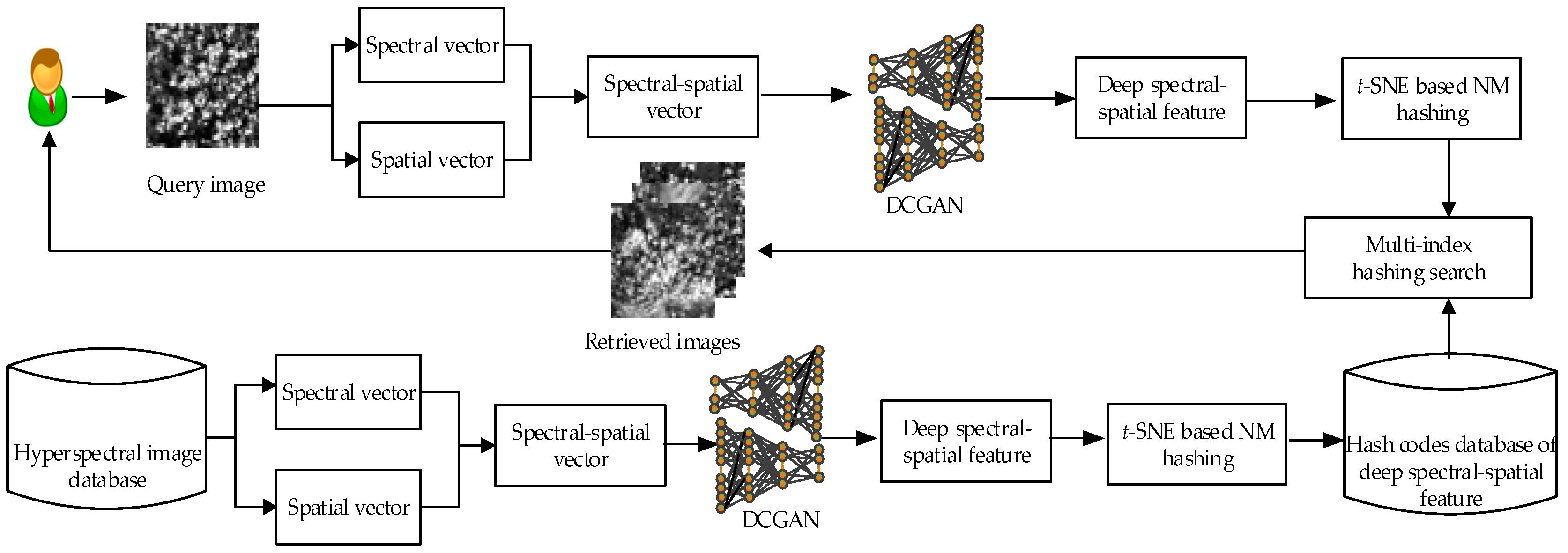
2. Our Proposed Method

The proposed hyperspectral image retrieval method mainly includes three parts: (1) deep spatial-spectral features are extracted from hyperspectral images by the DCGAN model; (2) t-SNE-based NM hashing method is utilized for dimensionality reduction of deep spectral-spatial features by projecting the deep spatial-spectral features into compact binary codes; (3) multi-index hashing search method is explored to measure similarity in Hamming space for finding the similar images.

Figure 1 shows the framework of the proposed hyperspectral image retrieval method. Our method queries hyperspectral images from pixel-wise-based matching. Firstly, spectral vectors and spatial vectors of manually selected pure pixels are extracted to combine into the spectral-spatial vector as training samples of the DCGAN model. The pixels are sampled from query hyperspectral image and hyperspectral images in the dataset respectively by using a sliding window. Deep spatial-spectral features of sampled pixels are obtained respectively by using the trained DCGAN model. Then t-SNE-based NM hashing method is utilized for dimensionality reduction by projecting the deep spatial-spectral vector into binary hash codes. Finally, similar hyperspectral images are retrieved through pixel-wise-based matching with the multi-index hashing search method. Next, we will make a detailed description of the proposed retrieval method.

2.1. Deep Spectral-Spatial Feature Extraction with DCGAN

Hyperspectral images include not only visual features, but also the most significant spectral features and spatial features. The spectrum of a pixel contains important information for discriminating between different kinds of ground categories. The K × K neighbor pixels of chosen pixels as spatial vectors are selected from the three principal bands. Spatial vectors are the statistics of the pixels in a neighbor region, which record relative position information among the pixels [10]. Spectral vectors and spatial vectors have been proved to be significant for representing hyperspectral images [29]. Deep learning, the latest research in the field of machine learning, has brought new opportunities for hyperspectral image retrieval [12,13,14]. Since hyperspectral images acquire the spectrum of a scene from hundreds of narrow-wavelength ranges within the electromagnetic spectrum, including visible and invisible bands, the limited human visual system makes it difficult to obtain labeled samples. However, most of the deep-learning networks demand a large number of labeled samples to train the models. Recently, Deep Convolutional Generative Adversarial Network (DCGAN) proposed by Alec Radford has become one of the most popular deep-learning methods. The DCGAN model is composed of a generator and discriminator, which can effectively learn the image features jointly in unsupervised and supervised ways when the labeled data is scarce [30]. For hyperspectral imagery, undesired scattering from other objects may deform the spectral characteristics of the object of interest. Furthermore, other factors, such as different atmospheric scattering condition and intraclass variability, make it extremely difficult to extract the features of hyperspectral data effectively [13]. To address such issues, deep architecture is known as a promising option since it can potentially lead to more abstract features at higher levels, which are generally robust and invariant. Compared with low-level handcrafted features, such as color, texture, and shape features, deep spectral-spatial features extracted by using DCGAN can reveal the intrinsic properties of the original data. Therefore, it can effectively eliminate influence of surrounding environmental conditions, such as illumination. Furthermore, differently to common two-dimensional images, three-dimensional hyperspectral images cannot be trained with a DCGAN model directly. Therefore, considering the high dimensionality and abundant spectral information, deep spectral-spatial features are extracted as follows:

(1)

Obtain the spectral-spatial vectors. Spectral vectors and spatial vectors are extracted respectively, and then spectral-spatial vectors can be obtained by combining spectral and spatial vectors using a Vector Stacking (VS) approach;

(2)

Train the DCGAN model. The DCGAN model is trained by spectral-spatial vectors as training samples and then optimized by using the Adaptive Moment Estimation (Adam) algorithm [31];

(3)

Extract the deep spectral-spatial features with the DCGAN model. The samples of the pixels are taken from hyperspectral images with a sliding window. The spatial vector and spectral vector of sampled pixels are extracted with Step 1). Finally, deep spectral-spatial features are extracted with the trained DCGAN model.

The deep spectral-spatial feature extraction flowchart is shown in Figure 2. In Figure 2, the manual pixel selection is not related to the pixel selection using the sliding window, which is separately utilized in training and testing processes. Firstly, the spectral-spatial vectors of pure pixels are extracted as a training set after pure pixels are selected manually from the hyperspectral image dataset. Then, pixels are selected using the sliding window to sample the pixels regularly from the query image and the images in the dataset. At last, the spectral-spatial vectors of sampled pixels are extracted as the testing set.

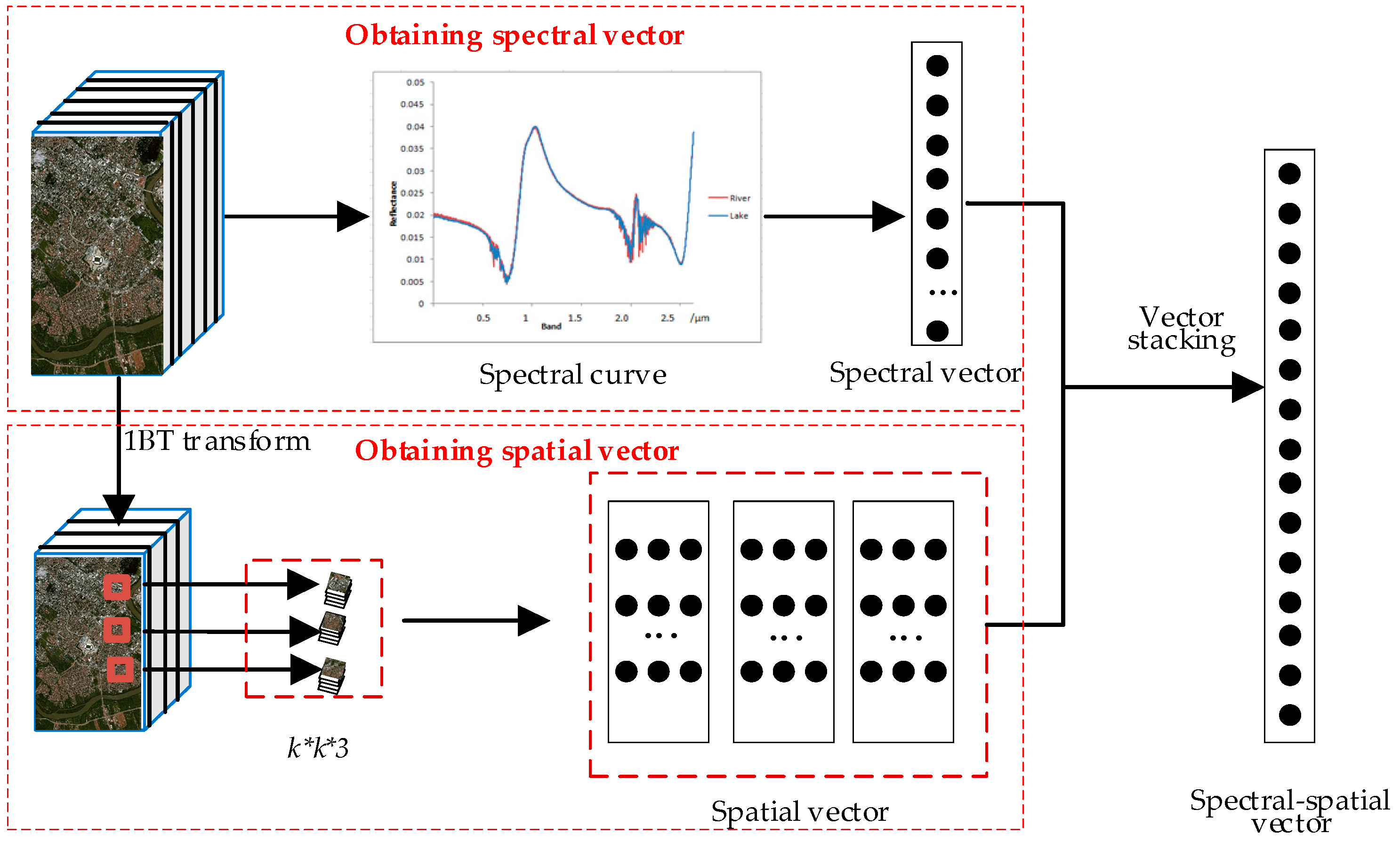
2.1.1. Obtaining Spectral-Spatial Vector

Pure pixels are acquired from the image in the same class of land-cover, which are the most spectrally unique or pure. That is to say, spectral vectors and spatial vectors of pure pixels are the most significant information in hyperspectral images. Therefore, we will combine pure pixels to form spectral-spatial vectors as training samples for each land-cover class. The obtaining process of spectral-spatial vectors is shown in Figure 3. Firstly, spectral vectors and spatial vectors are extracted respectively, and then spectral-spatial vectors can be obtained by combining the spectral vectors and spatial vectors using the Vector Stacking (VS) method. Next, we will introduce the detailed process of spectral and spatial vector extraction.

Spectral vectors are extracted directly by selecting the pure pixels manually from the images. For example, adjacently located pure pixels of a hyperspectral image are selected with a red box (see the river, soil, and plant in Figure 4a). Then, the red box is enlarged, and the pure pixels are fixed with a blue box in Figure 4b. Finally, the spectral vectors of pure pixels in the blue box are output directly. We connect pure pixels into a continuous spectral curve; the responding spectral curves of the river, soil and plant are shown in Figure 4c. Spatial vectors can be obtained by selecting the neighbor pixels of the pure pixels. Firstly, one-bit band image (1BT) representations of image bands are calculated for removing redundant information into hyperspectral images. 1BT representations of image bands, i.e., one-bit band images (1BTs), are obtained by filtering the image frames with a multi band-pass filter kernel. 1BTs can preserve important structure information of image bands, which is the basis for selecting the principal bands. Therefore, we need 1BT representations of image bands to preserve the structure information, in which the bands containing more structure information are selected as principal bands. Then, three principal bands of the hyperspectral image are selected after one-bit (1BT) transform. The specific processing can be divided into the following steps:

(1)

A multi band-pass filter kernel is used to filter the image frames for obtaining the one-bit band images (1BTs).

(2)

The spatial bit transitions A(l) in 1BTs (changes from 1 to 0, and vice-versa) are counted in horizontal and vertical directions.

(3)

The first three well-structured bands are selected as principal bands instead of the full bands by comparing the value of A(l) [32,33,34].

Finally, the spatial vectors of k × k neighbor pixels of pure pixels are extracted. After obtaining the spectral vectors and spatial vectors of pure pixels, a Vector Stacking (VS) approach is used to combine the spectral vectors with spatial vectors to form spectral-spatial vectors as training samples.

2.1.2. Training DCGAN Model

Since there is no public labeled dataset for hyperspectral retrieval, it is difficult to obtain a large number of labeled samples under the limitation of the human visual system. The DCGAN model is considered to have performed excellently. On the one hand, convolutional networks can effectively improve the feature-learning ability of discriminative networks; on the other, the network exhibits good convergence with shallow networks and fewer parameters when the labeled data is scarce. The DCGAN model includes two parts, i.e., a generator and a discriminator (see Figure 5). The generator is composed of a series of deconvolution layers, while the discriminator is composed of a series of convolution layers. In the generator, the output layer uses the tanh activation function while the other layers use the ReLU activation function. The tanh activation function selection in the output layer is determined based on the characteristics of tanh, which can be seen in Ref. [35]. Compared with ReLU, having no upper bound, tanh activation function is zero-centered with the range of [−1, 1], which is considered to have an advantage of expressive ability in the output layer. Just as in [35]: “We observed that using a bounded activation allowed the model to learn more quickly to saturate and cover the color space of the training distribution”. The size of convolution kernel is 5 × 5 with stride 2. All weights are initialized from a zero-centered normal distribution with standard deviation 0.02. The value of batch size and the epoch are set as 64 and 60. Batch Normalization (BN) and Leaky ReLU are used on each layer of the whole network except the input layer in the discriminator. The numbers of channels are halved, and the image dimension doubles from the previous layers in the discriminator; the generator is just the opposite. For the selection of kernel size, mini-batch size and feature map depth, we refer to the works in [16,30] to set the kernel size, mini-batch size, and feature map depth during training of the DCGAN model. For kernel size, when the size is smaller, the number of parameters and computational complexity can be greatly reduced without affecting the scope of the receptive field. This means that a smaller kernel size is able to consider information from as large an area of the original input volume as a bigger one. In comparison with other sizes during training, the kernel is set to 5 × 5 in this paper. In order to maximize the use of computer memory and ensure the descent direction accuracy, we try to increase the value of the mini-batch size. However, as the mini-batch size increases, the number of iterations decreases, and the time cost increases dramatically while achieving the same accuracy. Based on the aforementioned analysis, the mini-batch size is set to 64 in this paper. The value of the feature map depth is selected based on other formal studies and individual experience. We refer to [16] to set the value of feature map depth.

The DCGAN model is trained as follows:

(1)

Normalize all training samples to the range of [−1, 1] using the tanh activation function. In the generator, the output layer uses the tanh activation function. It means that the generated sample is normalized to the range of [−1, 1] by the tanh activation function through the output layer. After that, the generated samples and training samples need to be put into the discriminator respectively. Finally, the discriminator outputs the probability value that the input sample is real training data. To be consistent with the generated samples, all the training samples need to be scaled to the range of [−1, 1] with the tanh activation function before being put into the discriminator:

$$\mathrm{tanhx}=\frac{1-e^{-2\mathrm{x}}}{1+e^{-2\mathrm{x}}}$$

(1)

(2)

Train all models using mini-batch Stochastic Gradient Descent (SGD) with a mini-batch size of 64. All weights of parameters in the DCGAN model are initialized from a zero-centered normal distribution with standard deviation 0.02.

(3)

Generate the image g(Z) is by using a generator. First, the uniform distribution of the 100-dimensional noise vector Z is input into the generator, and then the Z is reshaped for the 4 × 4 × 1024 dimensional image through the full connection layer to finally generate the image after four times deconvolution.

(4)

Put the generated image g(Z) and the training image h into the discriminator network respectively. In the discriminator, a four-convolution layer and a fully connected layer are used to output a probability value that the input sample is real training data.

(5)

Calculate the loss V(G,D) of generated image g(Z) and the training image h in the discriminator, and update the variables in the generator and discriminator. The loss V(G,D) can be calculated as follows:

$$\underset{G}{\min } \underset{D}{\max } V(G,D)=E_{h\to p_{data}}\left[\log (D(h\left)\right)\right]+E_{Z\to p_{Z\left(x\right)}}\left[\log (-D(g(Z)\left)\right)\right]$$

(2)

where h is the training sample from the P_data distribution, Z is randomly selected from a 100-dimensional uniform distribution, G is the generative model and D is the discriminative model. As for (2), simply stated, G is updated to fool D into mistakenly judging the generated sample g(z), while D tries not to be fooled.

In order to further improve the accuracy of model, the parameters of the generator and discriminator model are optimized by the Adam algorithm [31]. The learning rate of each parameter is dynamically adjusted by the first moment estimation and second moment estimation of the gradient.

2.1.3. Deep Spectral-Spatial Feature Extraction

After training the DCGAN model, the deep spectral-spatial feature of each pixel in the hyperspectral image can be extracted. Considering the high dimensionality and abundant spectral and spatial information, the feature dimensions of an image will be as high as hundreds of thousands, and more if calculating all the pixels in the image. In order to effectively reduce the feature dimensionality while not dropping the descriptive ability, we choose an m × m sliding window to scan the image with the step size of s, which can be used to take samples of the pixels from images, as shown in Figure 6.

Next, spectral-spatial vectors as training samples are obtained by combining spectral vectors with spatial vectors by using the VS approach. After training the DCGAN model, the sampled pixels of the query image and images in database are put into the trained DCGAN respectively. The features are pooled in each layer by using a 4 × 4 pooling window, cascading all the features of all layers into a vector, which is used as a representation of the contents of the whole image. The deep spectral-spatial features containing high-level semantic information can be extracted through the aforementioned processes. For more details about deep spectral-spatial feature extraction, please refer to our previous work [36].

2.2. Dimensionality Reduction of Deep Spectral-Spatial Features by Using the t-SNE-Based Nonlinear Manifolds Hashing Method

Hashing-based dimensionality reduction has attracted more attention due to its highly efficient search within huge data archives and high data storage capability. Recently, learning-based hashing methods have been developed with the goal of learning more compact hash codes, including linear manifold learning and nonlinear manifold learning hashing. Nonlinear manifold learning methods are considered to preserve the local structure of the input data more effectively without assuming global linearity. However, there are two problems preventing the efficiency of manifold learning for hashing. In order to best preserve the semantic information, t-SNE is applied into the nonlinear manifold learning hashing method. t-SNE provides an effective technique for visualizing data and dimensionality reduction, which is capable of preserving local structures in high-dimensional data while retaining some global structures [25]. In order to reduce computational complexity as well as ensure the retrieval accuracy of a larger dataset, we select a representative small base set instead of the entire dataset to participate in dimensionality reduction by using t-SNE. Then, the low-dimensional embedding of the entire dataset can be obtained by using the inductive learning framework [20]. The steps of the t-SNE-based NM hashing project are divided into: (1) Fuzzy C-Means (FCM) clustering method, which is applied into dataset Y{y₁, y₂,…, y_n} to obtain a base set C (c₁, c₂, …, c_m), in which c_i (i = 1, 2, …, m) is the clustering center; (2) C (c₁, c₂,…, c_m), which is embedded into the low-dimensional space using the t-SNE method; (3) the low-dimensional embedding Y for the whole dataset, which is obtained using the inductive learning framework; and (4) Y, which is compared with the threshold zero to obtain the hash codes [20]. The details about the processing is as follows:

(1)

The FCM clustering method is utilized to partition Y{y₁, y₂, …, y_n} observations into m clusters C (c₁, c₂, …, c_m), in which each observation belongs to the cluster with the nearest mean [37].

(2)

The t-SNE method is applied into C (c₁, c₂, …, c_m) to obtain its low-dimensional embedding E_C{E₁, E₂,…,E_m}.

∙

Kullback-Leibler divergences is utilized to measure the faithfulness with the symmetrized conditional probability p_ij in the high-dimensional space and the joint probability q_ij defined using t-distribution in the low-dimensional embedding space.

∙

Then Ec can be obtained by minimizing Kullback-Leibler divergence over cluster center C using a gradient descent method. Kullback-Leibler divergence is a quantitative measurement of the information loss when choosing an approximation; ${\displaystyle \sum _{c_i\in C}{\displaystyle \sum _{c_j\in C}{p}_{ij}}}\log (\frac{p_{ij}}{q_{ij}})$ means relative entropy, representing the lost information.

∙

The low-dimensional embedding E_C can be obtained by minimizing the value of Kullback-Leibler divergence.

$$\underset{E_C}{\min }{\displaystyle \sum _{c_i\in C}{\displaystyle \sum _{c_j\in C}{p}_{ij}}}\log (\frac{p_{ij}}{q_{ij}})$$

(3)

(3)

The low-dimensional embedding $E_Y(E_{y_1},E_{y2},\dots ,E_{y_n})$ for the entire dataset Y{y₁, y₂, …, y_n} can be computed by (4), which is an inductive formulation derived from the inductive learning framework, as in [20]. The low-dimensional embedding E_Y can be computed with all cluster centers instead of the entire dataset Y because cluster centers have the overall weight with respect to the neighboring points.

$$E_{y_i}=\frac{{\displaystyle \sum _{j=1}^{m}w(y_i,c_j)E_j}}{{\displaystyle \sum _{j=1}^{m}w(y_i,c_j)}}$$

(4)

where w(y_i, c_i) is the element of graph affinity matrix that denotes the similarity correlation between data point y_i and cluster center c_j, which can be predicted as:

$$w(y_i,c_j)=\{\begin{array}{l}\exp (-{\Vert y_i-c_j\Vert }^2)/{\sigma }^2,c_j\in N\left(y_i\right)\\ 0,\mathrm{otherwise}\end{array}$$

(5)

where N(y_i) is the neighbor of y_i, and σ is the bandwidth parameter.

(4)

After obtaining the embeddings $E_{y_i}$ of samples y_i, the hash codes h(y_i) for the entire dataset Y{y₁, y₂, …, y_n} can be easily binaried by using (6).

$$h\left(y_i\right)=\mathrm{sgn}\left(E_{y_i}\right)$$

(6)

2.3. Similarity Measurement with Multi-Index Hashing in Hamming Space

As mentioned above, there are two ways to make a similarity measurement in Hamming space. However, it turns out that the traditional hashing method will consume a large amount of storage space in the retrieval process meaning that too much time is cost in searching for a similar process [25]. For example, for l bit hash code, the total number hash buckets is 2^l, the number Num of hash buckets to be examined when the radius is less than r is:

Num = C(l, 0)+C(l, 1)+...+C(l, r)

(7)

where C(l, i) (i = 0, 1, 2, …, r) is the hash buckets number with the radius i. However, Num will grow very rapidly with r, which greatly increases the time and storage complexity.

In order to solve the problems mentioned above, recently, a fast exact search method in Hamming space, i.e., multi-index hashing, is proposed [28]. It has proven that for uniformly distributed binary codes of l bits, the query time is sub-linear in the size of dataset with a search radius r when r/l is small. The similarity match process of the multi-index hashing for r-neighbor search can be divided into two parts:

(1)

Hash table building.

∙

Divide the length of hash code b into m disjointed substrings. The length of each substring is b/m, i.e., it is indexed m times into m different hash tables.

∙

Insert the hash code into jth (j = 1, 2, …, m) hash table. There are 2^b/m hash buckets in each hash table, and the total number of hash buckets H for the entire hash code is m × 2^b/m, which is much less than 2^b.

(2)

r-neighbor search.

For query substring q^j (j = 1, 2, …, a + 1, a + 2, …, m):

∙

When j = 1 to a + 1, look up the neighbors of q^j(j = 1, …, a + 1) with radius less than r’ in jth substring of H, in which the substring radius r’ and parameter a can be calculated as [28]:

r’ = ⌊r/m⌋, a = r − mr’

(8)

∙

When j = a + 1 to m, look up the neighbors of q^j(j = a + 2, …, m) with radius less than r’ − 1 in jth substring of H.

∙

Merge the m substrings and remove the non r-neighbors to obtain the r-radius neighbors of q^j.

Top-N similar hyperspectral images can be obtained from r-radius neighbors as follows: if the number M of retrieved hyperspectral images within lookup radius r₁ − 1 is less than N, and greater than N within lookup radius r₁, first N − M hyperspectral images can be selected from the lookup radius r₁+1 candidates by comparing the Euclidean distance of deep spectral-spatial features. In this way, we can obtain the retrieved Top-N similar hyperspectral images.

3. Experimental Results and Analysis

In this section, a quantitative study and comparative analysis are conducted to demonstrate the effectiveness of the proposed hyperspectral image retrieval method. In Experiment I, top-10 hyperspectral retrieval images are used for subjectively evaluating the descriptive ability of deep spectral-spatial features. In Experiment II, in order to objectively demonstrate that the descriptive ability of deep spectral-spatial features is stronger, the precision-recall curves and average precision ratios of four other feature-extraction methods, including our previous work APPI [5], the spectral and spatial feature extraction method [6], the EIA method [38] and deep spectral-spatial feature extraction with DBN [39] are compared. In Experiment III, comparative results in mean of average precision (MAP) with the other three state-of-the-art hash methods, i.e., spectral hashing [40], self-taught hashing [41], and graph hashing [42] are given. In Experiment IV, we compare the time cost of similarity comparison and retrieval accuracy before and after the hashing dimensionality reduction. Experiment V makes an analysis about precision-recall curves, time complexity, and space complexity among multi-index hashing searches and the other two similarity measurement methods, hamming distance rank [43] and original hash lookup methods [44].

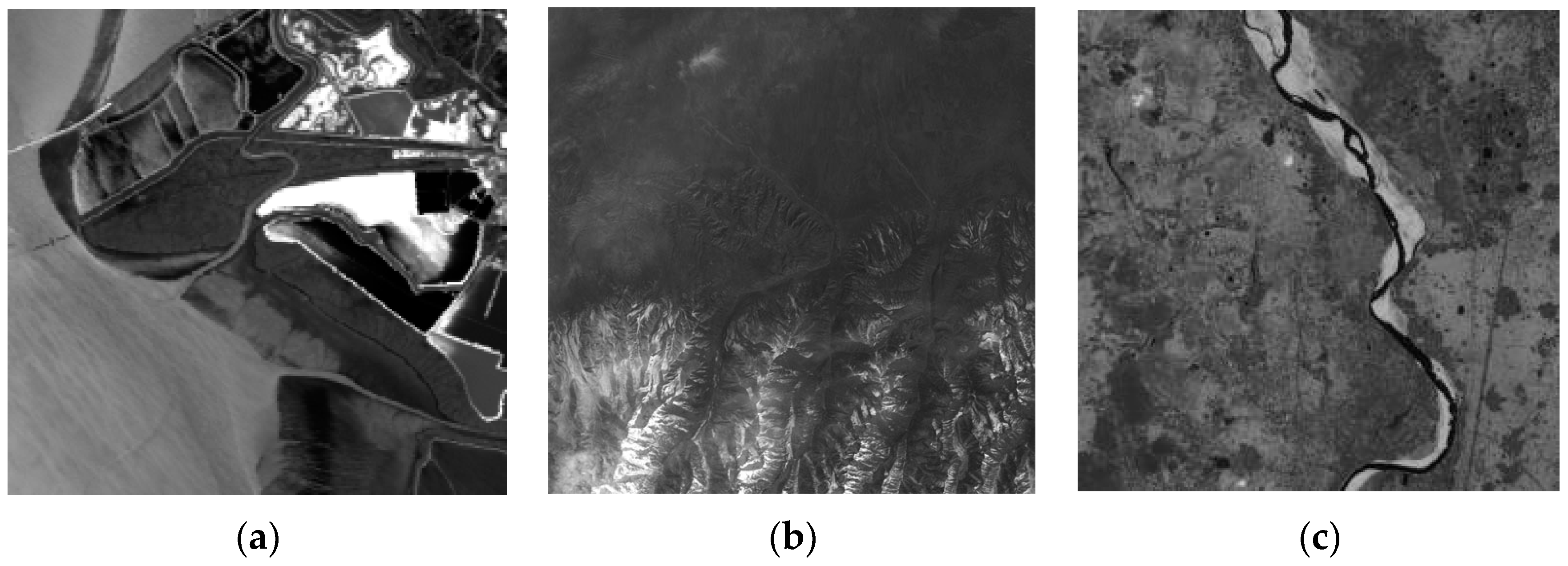
3.1. Experimental Dataset and Setting

The experiment of hyperspectral image retrieval is conducted on the high-resolution dataset of NASA data, which contains 224 spectral bands between 0.4 and 2.5 um. The spatial resolution is 20 m, and the spectral resolution is 10 nm. Figure 7 shows several sample images in the dataset, such as plain, rock and river. The experimental platform is a PC with 3.30 GHz CPU, 4.00 G memory, Linux operating system, NVIDIA GeForce GTX1080 GPU, Windows 7 operating system, MATLAB.

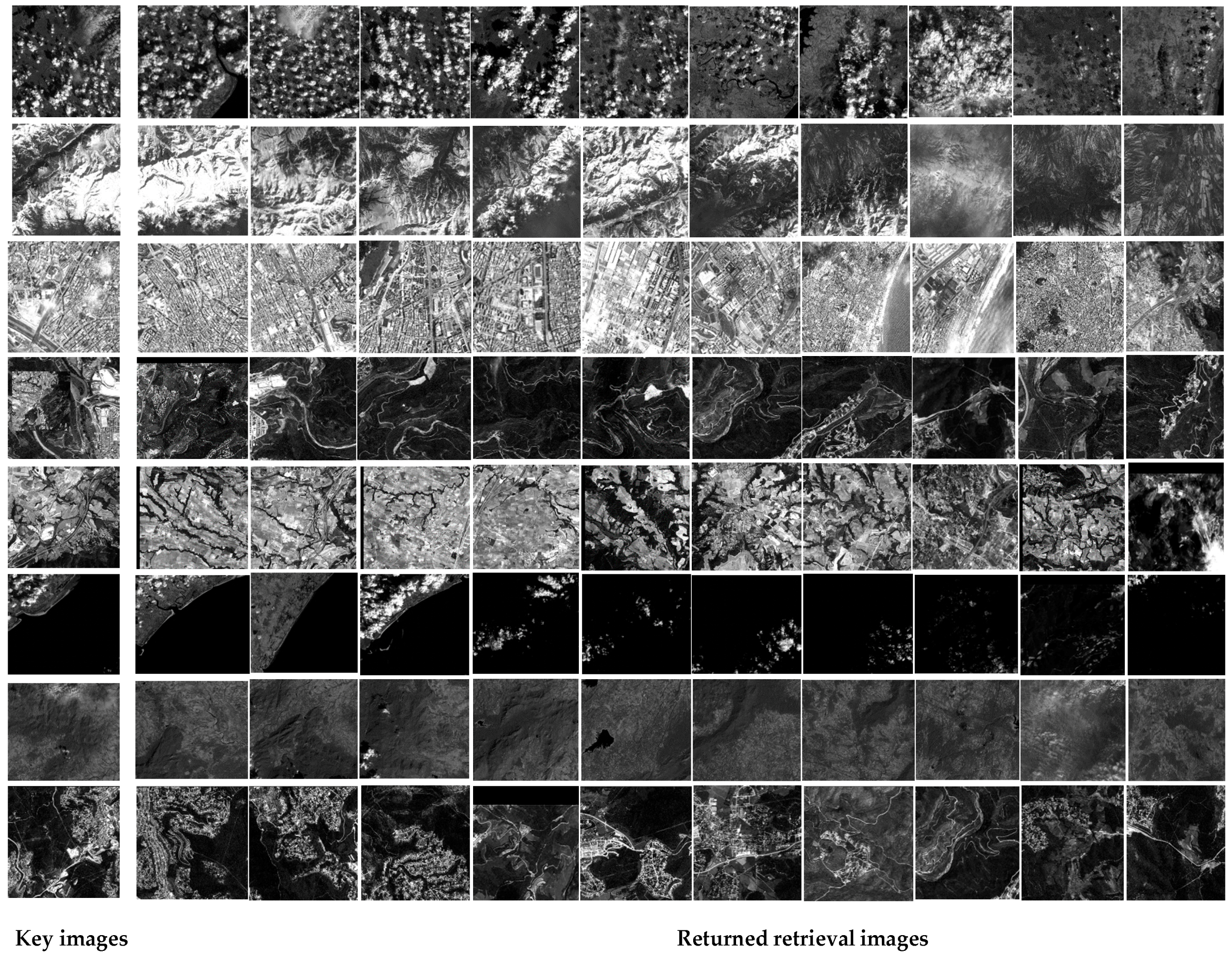
3.2. Experiment I: Top-10 Retrieved Hyperspectral Images Based on Deep Spectral-Spatial Feature

In this experiment, deep spectral-spatial features are used for hyperspectral image retrieval. Top-10 hyperspectral image retrieval results for a key image based on deep spectral-spatial features are shown in Figure 8. We can see that most of the retrieval images are similar to the key images.

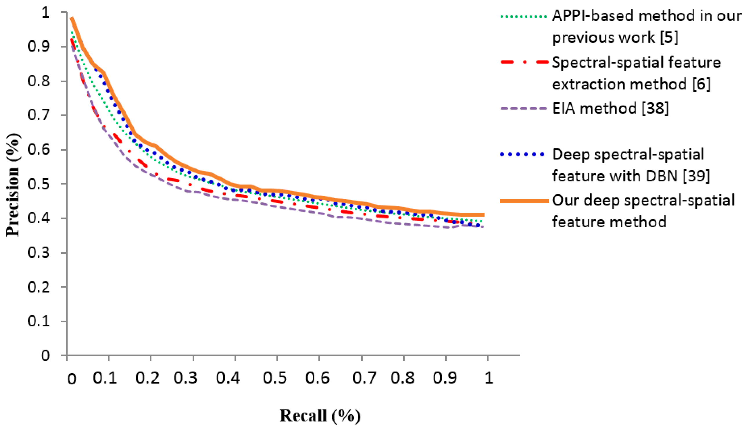
3.3. Experiment II: The Precision-Recall Curves and Average Precision Ratios Analysis of Deep Spectral-Spatial Features

The experiments of hyperspectral image retrieval are conducted to demonstrate the effectiveness of deep spectral-spatial features based on the DCGAN network. We compare this with our previous work APPI [5], the spectral and spatial features extraction method [6], the EIA method [38], and deep spectral-spatial feature extraction with DBN [39]. Similar to the DCGAN, DBN can also train in joint-supervised and unsupervised way. In this experiment, to make quantitative analysis of the hyperspectral image retrieval methods, the precision and recall curves are calculated. The definition of precision and recall can be denoted as:

$$\mathrm{Precision}=\frac{SIR}{SIR+NSIR}$$

(9)

$$\mathrm{Recall}=\frac{SIR}{SIR+SINR}$$

(10)

where the SIR is the number is similar images retrieved, NSIR is the number of non-similar images retrieved, SINR is the number of similar images not retrieved. The precision and recall curves of four methods are shown in Figure 9. As can be seen from Figure 9, the precision-recall curve of our method using deep spectral-spatial features can achieve a higher retrieval performance.

Table 1. The average precision ratios of four different methods.

Feature Extraction Methods	APPI in our Previous Work [5]	Spectral-Spatial Features [6]	EIA [38]	Deep Spectral-Spatial Features with DBN [39]	Our Deep Spectral-Spatial Feature
Average precision ratios (%)	78.49	73.22	73.18	81.33	86.49

shows the average precision ratios of four different methods, in which our method achieves 86.49%, superior to 78.49% in [5], 73.22% in [6], 73.18% in [38] and 81.33% in [39]. It further shows that our deep spectral-spatial features with DCGAN are more powerful in hyperspectral image retrieval. It is mainly because deep spectral-spatial features extracted with DCGAN have a stronger descriptive ability than other features.

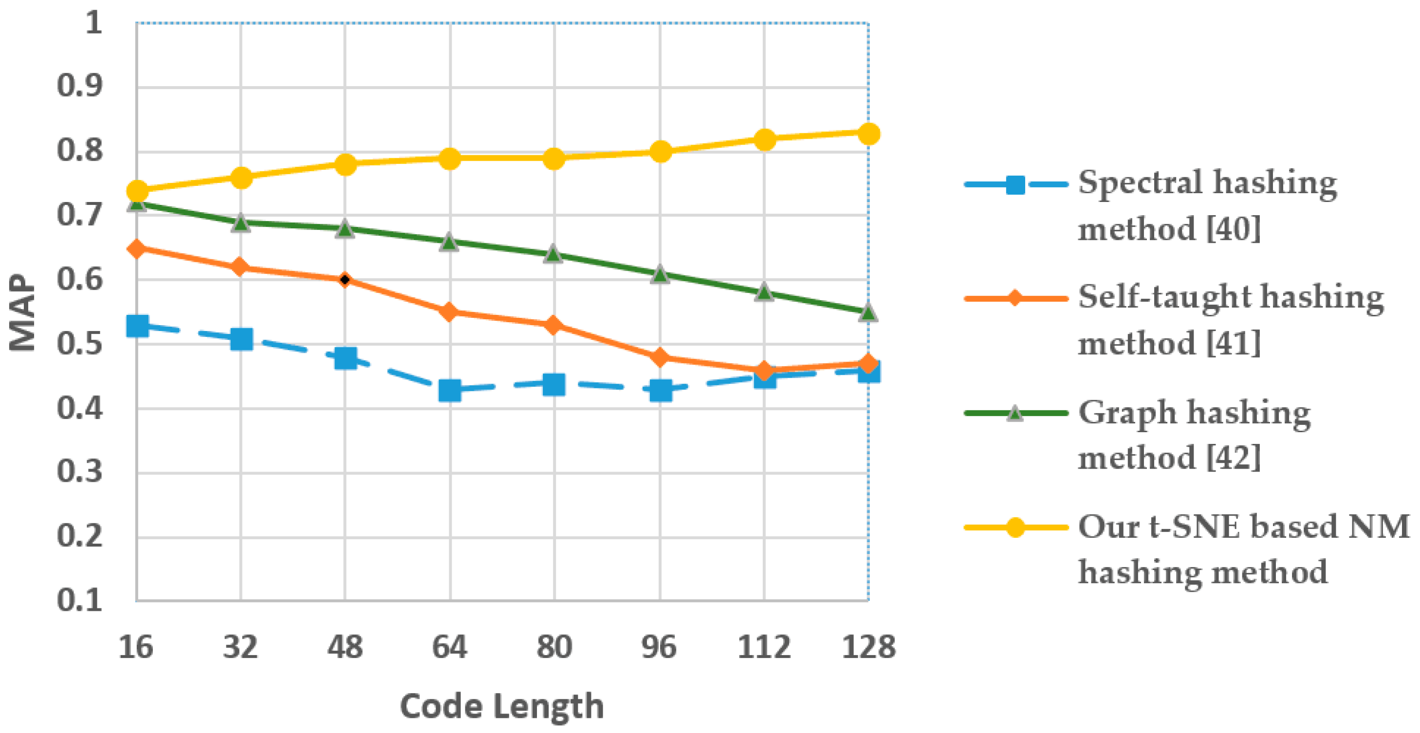
3.4. Experiment III: MAP Scores Analysis after Dimensionality Reduction of Hashing

As mentioned, the trade-off between recall and precision means both of them should be considered simultaneously when evaluating and comparing different retrieval algorithms. A popular measure taking recall, precision and order into account in returned images is the mean of average precision (MAP). MAP is the mean of the average precision scores for each query by using (11):

$$\mathrm{MAP}=\frac{{\displaystyle \sum _{d=1}^Q{\displaystyle \sum _{k=1}^{n}p\left(k\right)\Delta r\left(k\right)}}}{Q}$$

(11)

where Q is the number of queries, d is the serial number of queries, k is the rank in the sequence of retrieved images, n is the number of retrieved images, p(k) is the precision at cut-off, Δr(k) is the change in recall from items k − 1 to k. Figure 10 reports the comparative results of four hashing-based dimensionality-reduction methods using MAP: t-SNE-based NM hashing, spectral hashing [40], self-taught hashing [41] and graph hashing [42]. As can be seen from Figure 10, our t-SNE-based NM hashing method can perform better than the other three methods.

Table 2. The MAP of four methods with the 64-bit hash code.

Methods	Spectral Hashing [40]	Self-Taught Hashing [41]	Graph Hashing [42]	Our t-SNE Based NM Hashing
MAP (64 bits)	43.50%	54.90%	66.45%	79.20%

shows the MAP of the four methods with the 64-bit hash code, in which the MAP of our method is 79.20%, which is superior to 66.45% in [40], 54.90% in [41], and 43.50% in [42]. This is mainly because, compared with the other three hashing methods, t-SNE provides a more effective technique for preserving local structures in high-dimensional data while retaining some global structures and semantic information.

3.5. Experiment IV: Time Complexity and Average Precision Ratio Analysis before and after Dimensionality Reduction

In this experiment, the time cost, except for feature extraction (because the time cost of feature extraction before and after dimensionality reduction is the same), and the precision ratios of retrieval before and after the dimensionality reduction of deep spectral-spatial features are compared (see

Table 3. The time cost and average precision ratios for retrieval before and after the dimensionality reduction of deep spectral-spatial features.

Features	Original Feature	Hash Feature (64 bits)
Time cost (s)	1860	11.3 + 4.5 × 10−5
Average precision ratios (%)	86.49	86.10

). As can be seen from Table 3, the time cost of similarity comparison (1860 s) before dimensionality reduction is more than 150 times the time cost of dimensionality reduction (11.3 s) and similarity comparison (4.5 × 10⁻⁵ s) after dimensionality reduction, while the retrieval accuracy using t-SNE-based NM hashing method is 86.10%, which is slightly lower than using the original deep feature 86.49%. The main reason is that the comparison of the two values in Hamming space with very short code length greatly reduces the computational complexity. Moreover, t-SNE preserves the local structures while retaining some global structures.

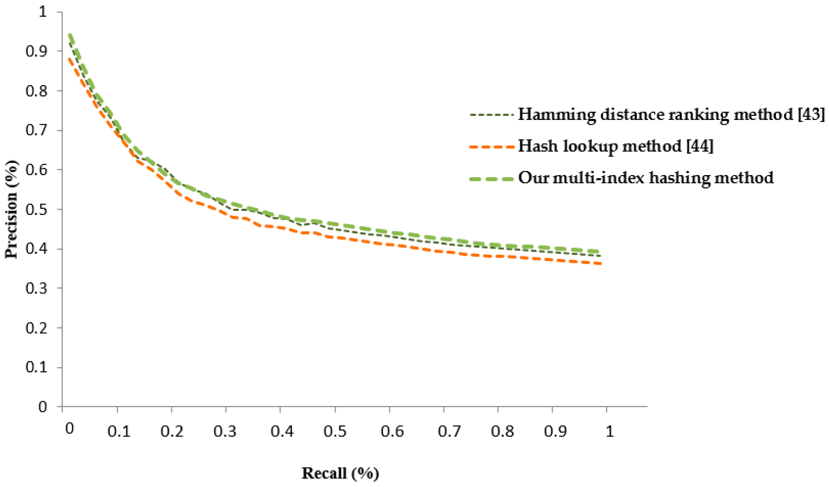
3.6. Experiment V: Precision-Recall Curves, Time Cost and Storage Complexity Analysis of Multi-Index Hashing

In this experiment, the precision-recall curves of multi-index hashing, Hamming distance ranking and the original hash lookup methods are compared in Figure 11. The average precision ratios of the three methods are shown in

Table 4. The average precision ratios of multi-index hashing and other hash rank methods.

Methods	Hamming Rank [43]	Hash Look Up [44]	Our Multi-Index Hashing
Average precision ratios (%)	79.33%	77.50%	80.60%

. The time cost and storage complexity of the three methods are shown in

Table 5. The time cost and space complexity for different search methods in Hamming space (q is the length of hash codes, N is the number of the dataset, m is the number of substrings).

Methods	Hamming Rank [43]	Hash Look Up [44]	Our Multi-Index Hashing
Time cost (s)	4.5 × 10−5	5.0 × 10−7	5.8 × 10−8
Space complexity	O(N × q)	O(q × 2q)	O(q × 2q/m)

. We set Hamming radius to be 6 and the hash code is 64 bits. From Figure 11, we can see that the precision-recall ratio curves of the three methods almost coincide with each other, in which the average precision ratios of our multi-index hashing method is 80.60%, a little superior to 79.33% in [43], 77.50% in [44]. The main reason for this is that the returned candidate sets of the three methods are both obtained by computing the Hamming distance. Morever, we can see from Table 5 that the time cost 5.0 × 10⁻⁷ s of original hash lookup is about 10 times less than, and the Hamming distance ranking 4.5 × 10⁻⁵ s is about 300 times less than multi-index hashing, which is very effective for allowing us to enlarge our dataset in future work. Furthermore, the space complexity of our multi-index hashing O(q × 2^q/m) is far less than the hamming rank O(N × q) and the original hash lookup O(q × 2^q) (Table 5), especially in the condition of the longer hash codes.

4. Discussion

We have proposed an efficient method for hyperspectral image retrieval in this paper. The approach works to improve the hyperspectral retrieval performance from two aspects: retrieval accuracy and retrieval efficiency. In terms of retrieval accuracy, taking into account the characteristics of hyperspectral images, deep spectral-spatial features are extracted by using the DCGAN model in an unsupervised way to enhance the descriptive ability of representing the hyperspectral image. In terms of retrieval efficiency, two improvements are made: (1) the dimensionality reduction of deep spectral-spatial features. Deep spectral-spatial features usually have up to thousands of dimensionalities, which greatly affect the retrieval efficiency. Manifold learning-based hashing techniques are better able to model the intrinsic structure embedded in the original high-dimensional data. Specially, nonlinear manifold learning-based hashing methods are more powerful at preserving the local structure of the input data. In order to improve the retrieval efficiency while preserving the local structure and semantic information, t-SNE-based NM hashing is adopted for the dimensionality reduction of deep spectral-spatial features; (2) the similarity measurement of hyperspectral image features. The most popular similarity measurement in Hamming space is the hash lookup. However, there is a problem that affects retrieval efficiency in the original hash lookup method, i.e., the number of distinct hash buckets are proved to grow rapidly with hash codes. The mass of storage space is wasted because many hash buckets are empty. Multi-index hashing can solve this problem by dividing the hash codes in to short substrings. In this way, retrieval efficiency can be further improved.

Five experiments are conducted to verify the effectiveness of our proposed method. Experiment I returns top-10 retrieved hyperspectral images for subjectively evaluating the descriptive ability of deep spectral-spatial features. In Figure 8, we can see that most of the retrieval images are similar to the key images. It reveals that deep spectral-spatial features have a powerful descriptive ability. Experiment II evaluates the descriptive ability of deep spectral-spatial features from an objective perspective. As illustrated in Figure 9 and Table 1, deep spectral-spatial features of hyperspectral images extracted by using the DCGAN model can perform better than the other four state-of-the-art methods. Our method is 8 percentage points superior to APPI in our previous work [5], 13.27 percentage points superior to spectral-spatial feature [6], 13.31 percentage points superior to EIA [38], and 5.16 percentage points superior to deep spectral-spatial features with DBN [39]. The main reasons include: (1) the methods [5,6,38] extract the low-level handcrafted features of a hyperspectral image, such as the endmember features, spectral features, and spatial features. Our deep spectral-spatial features are extracted through a four-convolution layer in the discriminator of DCGAN, containing deep semantic information. The descriptive ability of our deep spectral-spatial features is obviously more powerful. The deep spectral-spatial features with DBN in [39] has lower descriptive ability because the size of the dataset is relatively small for the DBN model; (2) the methods in [5,6,38] extract regional-level features from the hyperspectral image, including local and global features, while our deep spectral-spatial features are extracted from hyperspectral images at the pixel level, which is more precise and complicated. The method in [39] extracts deep spectral-spatial features without considering the structure information of the pixels because the input of DBN is a one-dimensional vector. While the convolution layer tackles with the two-dimensional structure, it can more effectively learn the structure information through convolution operation. In Experiment III and Experiment IV, retrieval performance is assessed by using deep hash codes after dimensionality reduction with the t-SNE-based NM hashing method. Figure 10 and Table 2 suggests that our t-SNE-based NM hashing method can perform better than spectral hashing [40], self-taught hashing [41] and graph hashing [42] in MAP. From Table 2, the MAP of our method is 35.70 percentage points superior to spectral hashing in [40], 24.30 percentage points superior to self-taught hashing in [41], and 12.75 percentage points superior to graph hashing in [42]. Time cost and average precision ratio analysis before and after dimensionality reduction are observed in Table 3. Although the original deep spectral-spatial features for hyperspectral image retrieval are shown to be only slightly higher than using the t-SNE-based NM hashing method, analysis of time cost shows that the performance of our t-SNE-based NM hashing method tends to provide a bigger advantage compared to the original deep spectral-spatial features. The main reasons for the above results are: (1) spectral hashing, graph hashing and self-taught hashing would destroy the manifold structure of deep spectral-spatial features in dimensionality reduction processing, while our t-SNE provides a more effective technique for preserving local structures and semantic information in high-dimensional data; (2) the similarity comparison between binary codes can speed up the search efficiency enormously. Experiment V computes the precision-recall curves, time cost and storage complexity analysis of using multi-index hashing. Compared with the similarity measurement results as illustrated in Figure 11, and Table 4 and Table 5, our multi-index hashing can obviously reduce the time cost and the space complexity for similarity measurement when the precision-recall ratio curves of the three methods almost coincide with each other. The main reasons include: (1) the returned candidate sets of the three methods are both obtained by computing the Hamming distance, therefore, the precision-recall ratio curves vary a little; (2) the multi-index hashing divides the long hash codes into short substrings so that the space complexity and the time cost of comparisons are reduced.

In the future work, firstly, we will reform the current deep learning models according to the characteristics of hyperspectral images, making them more suitable for extracting more accurate hyperspectral image features. Then we will merge the t-SNE-based NM hashing method into the deep learning model to form a whole framework; a series of hash codes after dimensionality reduction can be directly obtained when the hyperspectral image is input into the framework. In this way, it can simplify the processes of deep spectral-spatial extraction and dimensionality reduction. Finally, top-N similar hyperspectral images are selected from the radius r candidates by comparing the Euclidean distance of deep spectral-spatial features. However, the Euclidean distance comparison of deep spectral-spatial features is not efficient when the database is larger. Other similarity measurement methods for hash codes can be introduced to further improve the retrieval performance.

5. Conclusions

With the rapid development of Earth observation technology, remote imaging sensors with high spatial resolution have brought rapid growth in the volume of acquired hyperspectral images. Therefore, the effective management and retrieval of large-scale hyperspectral image datasets is increasingly becoming important. In this work, an efficient hyperspectral image retrieval method is proposed. To improve the descriptive ability of hyperspectral features, deep spectral-spatial features are extracted. In order to prove the descriptive ability of deep spectral-spatial features, the precision-recall curve and average precision ratios are compared with the other four state-of-the-art hyperspectral features. From the results, we can see that our deep spectral-spatial features achieve a better performance. Our method can extract high-level semantic features by using the DCGAN model. Considering that high-dimensional deep features greatly affect retrieval efficiency, the t-SNE-based NM hashing method is adopted for deep feature dimensionality reduction. The experiments on MAP scores are computed between our method and the other three hashing methods. From the experimental results, we can see that our t-SNE-based NM hashing method achieves a higher score. The main reason is that the t-SNE-based NM hashing method can preserve the local and global structure better than others. Finally, multi-index hashing in Hamming space is applied to find similar images to further lower the space complexity. The precision-recall curve, average precision ratios, time cost and space complexity are compared between multi-index hashing and the other two similarity measurement methods in Hamming space. From the results, we can see that our method can greatly reduce space complexity in the case of comparable retrieval performance.

References

1. Zhong, Z.; Fan, B.; Duan, J. Discriminant tensor spectral–spatial feature extraction for hyperspectral image classification. IEEE Geosci. Remote Sens. Lett. 2017, 12, 1028–1032. [Google Scholar] [CrossRef]
2. Zhang, E.; Zhang, X.; Yang, S. Improving hyperspectral image classification using spectral information divergence. IEEE Geosci. Remote Sens. Lett. 2014, 51, 249–253. [Google Scholar] [CrossRef]
3. Zhou, W.; Li, C. Deep feature representations for high-resolution remote-sensing imagery retrieval. Remote Sens. 2017, 9, 489. [Google Scholar] [CrossRef]
4. Shao, Z.; Zhou, W.; Cheng, Q. An effective hyperspectral image retrieval method using integrated spectral and textural features. Sens. Rev. 2015, 35, 274–281. [Google Scholar] [CrossRef]
5. Zhang, J.; Zhou, Q.L.; Zhuo, L.; Geng, W.H.; Wang, S. A CBIR system for hyperspectral remote sensing images using endmember extraction. Pattern Recognit. 2017, 31, 1752001. [Google Scholar] [CrossRef]
6. Graña, M. A spectral/spatial CBIR system for hyperspectral images. IEEE J. Sel. Top. Appl. Earth Obs. Remote Sens. 2012, 5, 488–500. [Google Scholar]
7. Ye, Z.; Tan, L.; Bai, L. Hyperspectral image classification based on spectral-spatial feature extraction. In Proceedings of the International Workshop on Remote Sensing with Intelligent Processing, Shanghai, China, 19–21 May 2017; pp. 489–499. [Google Scholar]
8. Deng, S.B. Image enhancement. In ENVI Remote Sensing Image Processing Method, 1rd ed.; Peng, S.C., Zhang, J.F., Eds.; Science Press: Beijing, China, 2010; ISBN 978703027600. [Google Scholar]
9. Li, C.; Ma, Y.; Mei, X.; Liu, C.; Ma, J. Hyperspectral image classification with robust sparse representation. IEEE Geosci. Remote Sens. Lett. 2017, 13, 641–645. [Google Scholar]
10. Zhu, Y.; Huang, X.; Huang, Q.; Tian, Q. Large-scale video copy retrieval with temporal-concentration sift. Neurocomputing 2016, 187, 83–91. [Google Scholar] [CrossRef]
11. Zhu, Y.; Jiang, J.; Han, W.; Ding, Y.; Tian, Q. Interpretation of users’ feedback via swarmed particles for content-based image retrieval. Inf. Sci. 2017, 375, 246–257. [Google Scholar] [CrossRef]
12. Li, Y.; Xie, W.; Li, H. Hyperspectral image reconstruction by deep convolutional neural network for classification. Pattern Recognit. 2017, 63, 371–383. [Google Scholar] [CrossRef]
13. Chen, Y.; Jiang, H. Deep feature extraction and classification of hyperspectral images based on convolutional neural networks. IEEE Trans. Geosci. Remote Sens. 2016, 54, 6232–6251. [Google Scholar] [CrossRef]
14. Chen, Y.; Zhao, X.; Jia, X. Spectral–spatial classification of hyperspectral data based on deep belief network. IEEE J. Sel. Top. Appl. Earth Obs. Remote Sens. 2015, 8, 2381–2392. [Google Scholar] [CrossRef]
15. Salman, M.; Yüksel, S.E. Hyperspectral data classification using deep convolutional neural networks. In Proceedings of the Signal Processing and Communication Application Conference, Budapest, Hungary, 29 August–2 September 2016; pp. 2129–2132. [Google Scholar]
16. Zhang, Z.; Liu, X.; Cui, Y. Multi-phase offline signature verification system using deep convolutional generative adversarial Networks. In Proceedings of the International Symposium on Computational Intelligence and Design, Hangzhou, China, 10–11 December 2016; pp. 103–107. [Google Scholar]
17. Han, M.; Zhang, C. Spectral-spatial classification of hyperspectral image based on discriminant sparsity preserving embedding. Neurocomputing 2017, 243, 133–141. [Google Scholar] [CrossRef]
18. Malik, M.R.; Isaac, B.J.; Coussement, A. Principal component analysis coupled with nonlinear regression for chemistry reduction. Combust. Flame 2017, 187, 30–41. [Google Scholar] [CrossRef]
19. Roweis, S.T.; Saul, L.K. Nonlinear dimensionality reduction by locally linear embedding. Science 2000, 290, 2323–2326. [Google Scholar] [CrossRef] [PubMed]
20. Huang, Q.; Feng, J.; Fang, Q. Query-aware locality-sensitive hashing scheme for norm. VLDB J. 2017, 26, 683–708. [Google Scholar] [CrossRef]
21. Shen, F.; Shen, C.; Liu, W. Supervised discrete hashing. In Proceedings of the International Conference on Computer Vision and Pattern Recognition, Boston, MA, USA, 7–12 June 2015; pp. 37–45. [Google Scholar]
22. Talwalkar, A.; Kumar, S.; Rowley, H.A. Large-scale manifold learning. In Proceedings of the International Conference on Computer Vision and Pattern Recognition, Anchorage, AK, USA, 24–26 June 2008; pp. 1–8. [Google Scholar]
23. Shen, F.; Shen, C.; Shi, Q. Hashing on nonlinear manifolds. IEEE Trans. Image Process. 2015, 24, 1839–1851. [Google Scholar] [CrossRef] [PubMed]
24. Gu, H.; Wang, X.; Chen, X. Manifold learning by curved cosine mapping. IEEE Trans. Knowl. Data Eng. 2017, 29, 2236–2248. [Google Scholar] [CrossRef]
25. Maaten, L.V.; Hinton, G. Visualizing data using t-SNE. J. Mach. Learn. Res. 2008, 9, 2579–2605. [Google Scholar]
26. Cakir, F.; Sclaroff, S. Adaptive hashing for fast similarity search. In Proceedings of the IEEE International Conference on Computer Vision, Boston, MA, USA, 8–10 June 2015; pp. 1044–1052. [Google Scholar]
27. Norouzi, M.; Punjani, A.; Fleet, D.J. Fast search in Hamming space with multi-index hashing. In Proceedings of the IEEE Conference on Computer Vision and Pattern Recognition, Providence, RI, USA, 16–21 June 2012; pp. 3108–3115. [Google Scholar]
28. Norouzi, M.; Punjani, A.; Fleet, D.J. Fast exact search in Hamming space with multi-index hashing. IEEE Trans. Pattern Anal. 2014, 36, 1107–1119. [Google Scholar] [CrossRef] [PubMed]
29. Zhu, Z.; Woodcock, C.E.; Rogan, J.; Kellndorfer, J. Assessment of spectral, polarimetric, temporal, and spatial dimensions for urban and peri-urban land cover classification using Landsat and SAR data. Remote Sens. Environ. 2012, 117, 72–82. [Google Scholar] [CrossRef]
30. Radford, A.; Metz, L.; Chintala, S. Unsupervised representation learning with deep convolutional generative adversarial networks. arXiv, 2015; arXiv:1511.06434. [Google Scholar]
31. Kingma, D.P.; Ba, J. Adam: A method for stochastic optimization. arXiv, 2014; arXiv:1412.6980. [Google Scholar]
32. Demir, B.; Celebi, A. A low-complexity approach for the color display of hyperspectral remote-sensing images using One-Bit-Transform-Based band selection. IEEE Trans. Geosci. Remote Sens. 2009, 47, 97–105. [Google Scholar] [CrossRef]
33. Natarajan, B.; Bhaskaran, V.; Konstantinides, K. Low-complexity block-based motion estimation via one-bit transforms. IEEE Trans. Circuits Syst. Video Technol. 1997, 7, 702–706. [Google Scholar] [CrossRef]
34. Urhan, O.; Erturk, S. Constrained one-bit transform for low complexity block motion estimation. IEEE Trans. Circuits Syst. Video Technol. 2007, 17, 478–482. [Google Scholar] [CrossRef]
35. Glorot, X.; Bordes, A.; Bengio, Y. Deep sparse rectifier neural networks. In Proceedings of the IEEE Conference on Artificial Intelligence and Statistics, Lauderdale, FL, USA, 11–13 April 2011; pp. 315–323. [Google Scholar]
36. Chen, L.; Zhang, J.; Liang, X.; Li, J.F.; Zhuo, L. Deep spectral-spatial feature extraction based on DCGAN for hyperspectral image retrieval. In Proceedings of the IEEE Conference on Pervasive Intelligence and Computing, Orlando, FL, USA, 6–10 November 2017; pp. 1–8. [Google Scholar]
37. Yang, M.S.; Nataliani, Y. Robust-learning fuzzy c-means clustering algorithm with unknown number of clusters. Pattern Recognit. 2017, 71, 45–59. [Google Scholar] [CrossRef]
38. Graña, M. An endmember-based distance for content based hyperspectral image retrieval. Pattern Recognit. 2012, 45, 3472–3489. [Google Scholar] [CrossRef]
39. Hinton, G.E.; Osindero, S.; The, Y.W. A fast learning algorithm for deep belief net. Neural Comput. 2014, 18, 1527–1554. [Google Scholar] [CrossRef] [PubMed]
40. Weiss, Y.; Torralba, A.; Fergus, R. Spectral hashing. In Proceedings of the International Conference on Neural Information Processing Systems, Vancouver, BC, Canada, 8–10 December 2008; pp. 1753–1760. [Google Scholar]
41. Zhang, D.; Wang, J.; Cai, D.; Lu, J. Self-taught hashing for fast similarity search. In Proceedings of the International ACM SIGIR Conference on Research and Development in Information Retrieval, Geneva, Switzerland, 19–23 July 2010; pp. 18–25. [Google Scholar]
42. Liu, W.; Wang, J.; Kumar, S.; Chang, S.F. Hashing with graphs. In Proceedings of the International Conference on Machine Learning, Washington, DC, USA, 28 June–2 July 2011; pp. 1–8. [Google Scholar]
43. Jegou, H.; Douze, M.; Schmid, C. Hamming embedding and weak geometric consistency for large scale image search. In Proceedings of the European Conference on Computer Vision, Marseille, France, 12–18 October 2008; pp. 304–317. [Google Scholar]
44. Liu, X.L.; Fan, X.J.; Deng, C.; Li, Z.J.; Su, H.; Tao, D.C. Multilinear hyperplane hashing. In Proceedings of the IEEE Conference on Computer Vision and Pattern Recognition, Paris, France, 26–27 September 2016; pp. 5119–5127. [Google Scholar]
Figure 1. The framework of the proposed retrieval method of hyperspectral imagery.
Remotesensing 10 00271 g001
Figure 2. The flow-chart of deep spectral-spatial feature extraction.
Remotesensing 10 00271 g002
Figure 3. The combination of spectral vectors and spatial vectors.
Remotesensing 10 00271 g003
Figure 4. The spectral vector extraction: (a) The pure pixels of river, soil and plant; (b) The pure pixels of river, soil and plant; (c) The spectral curve of river, soil and plant.
Remotesensing 10 00271 g004
Figure 5. The architecture of the generator and the discriminator in the DCGAN model.
Remotesensing 10 00271 g005
Figure 6. The visual reference of the sliding window.
Remotesensing 10 00271 g006
Figure 7. The samples of AVIRIS images. (a) The hyperspectral image of plain; (b) The hyperspectral image of rock; (c) The hyperspectral image of river.
Remotesensing 10 00271 g007
Figure 8. Hyperspectral image retrieval results.
Remotesensing 10 00271 g008
Figure 9. The precision-recall curves of different methods.
Remotesensing 10 00271 g009
Figure 10. The MAP of the four methods.
Remotesensing 10 00271 g010
Figure 11. The precision-recall curves of multi-index hashing and other hash rank methods.
Remotesensing 10 00271 g011