Shortwave IR Adaption of the Mid-Infrared Radiance Method of Fire Radiative Power (FRP) Retrieval for Assessing Industrial Gas Flaring Output


1
Department of Geography, King’s College London, Strand, London WC2R 2LS, UK
2
NERC National Centre for Earth Observation (NCEO), King’s College London, Strand, London WC2R 2LS, UK
*
Author to whom correspondence should be addressed.
Remote Sens. 2018, 10(2), 305; https://doi.org/10.3390/rs10020305
Submission received: 12 January 2018
/
Revised: 7 February 2018
/
Accepted: 10 February 2018
/
Published: 16 February 2018
(This article belongs to the Section Atmospheric Remote Sensing)
Abstract
:The radiative power (MW) output of a gas flare is a useful metric from which the rate of methane combustion and carbon dioxide emission can be inferred for inventorying purposes and regular global surveys based on such assessments are now being used to keep track of global gas flare reduction efforts. Several multispectral remote sensing techniques to estimate gas flare radiative power output have been developed for use in such surveys and single band approaches similar to those long used for the estimation of landscape fire radiative power output (FRP) can also be applied. The MIR-Radiance method, now used for FRP retrieval within the MODIS active fire products, is one such single band approach—but its applicability to gas flare targets (which are significantly hotter than vegetation fires) has not yet been assessed. Here we show that the MIR-Radiance approach is in fact not immediately suitable for retrieval of gas flare FRP due to their higher combustion temperatures but that switching to use data from a SWIR (rather than MWIR) spectral channel once again enables the method to deliver unbiased FRP retrievals. Over an assumed flaring temperature range of 1600–2200 K we find a maximum FRP error of ±13.6% when using SWIR observations at 1.6 µm and ±6.3% when using observations made at 2.2 µm. Comparing these retrievals to those made by the multispectral VIIRS ‘NightFire’ algorithm (based on Planck Function fits to the multispectral signals) we find excellent agreement (bias = 0.5 MW, scatter = 1.6 MW). An important implication of the availability of this new SWIR radiance method for gas flare analysis is the potential to apply it to long time-series from older and/or more spectrally limited instruments, unsuited to the use of multispectral algorithms. This includes the ATSR series of sensors operating between 1991–2012 on the ERS-1, ERS-2 and ENVISAT satellites and such long-term data can be used with the SWIR-Radiance method to identify key trends in global gas flaring that have occurred over the last few decades.
1. Introduction and Background
The rate of radiative heat release from landscape fire events is typically estimated using remotely sensed retrievals of Fire Radiative Power (FRP) e.g., [1,2,3]. FRP measures, established as a useful metric for indicating relative rates of vegetation fire smoke emission for the SCAR-B and SCAR-C airborne campaigns [4,5], were shown to be directly related to combustion rates in laboratory-scale experiments by [2], work subsequently followed up by further similar-scale experiments e.g., [6]. Subsequently FRP data have joined burned area methods (e.g., [7,8]) in being used to further the understanding of numerous environmental and global change processes modulated by landscape fires, including rates of fuel consumption and trace gas and aerosol emission, e.g., [2,9,10,11,12,13,14]. Many different EO (Earth Observation) instruments have been employed in such efforts and multiple algorithms developed for the detection of actively burning fires and determination of their FRP e.g., [1,10,15,16,17,18,19,20,21,22,23]. One of the most widely used FRP retrieval approaches is the Mid-Infrared (MIR-) Radiance method, developed in [1,2], now used for FRP derivation within NASA’s widely used Moderate Resolution Imaging Spectro-radiometer (MODIS) MOD14/MYD14 active fire products [24], as well as fire products from the geostationary SEVIRI and the GOES imagers [18,25] and the polar orbiting Sentinel-3 Sea and Land Surface Temperature Radiometer (SLSTR) [19]. Whilst the MIR-Radiance method is applied at land— (and sometimes ocean—) based gas flare hotspots in these products, its validity has yet to be tested for these types of target. Landscape biomass burning typically involves radiating temperatures in the range ~650–1300 K e.g., [26,27], with the peak of their spectral radiant energy emission therefore occurring in or very close-to the middle infrared (MIR) spectral region (in accordance with Wien’s Displacement Law e.g., [1,28]). Combustion of natural gas at sites of industrial flaring typically results in radiant temperatures hundreds of Kelvin higher, usually exceeding 1600 K [20]. This higher temperature shifts their spectral emission peak well into the shortwave infrared (SWIR) spectral region when compared to that of vegetation fires [29] and so adaptations to the MIR-Radiance method may well be required to maintain accuracy when the approach is applied at gas flare locations. This is important because FRP retrievals made at gas flare targets can be used for the estimation of rates of methane consumption and carbon dioxide emission [23,30] and inventories produced using such approaches can support global gas flaring greenhouse gas (GHG) reduction efforts [31,32]. Fairly recent analyses have estimated that flaring contributes around 1.2% of global anthropogenic CO2 emissions [33], whilst also releasing air pollutants such as black carbon, sulphur dioxide, nitrogen oxides and hydrogen sulphide [34,35].
A key advantage of the MIR-Radiance method is its use of only single waveband data to retrieve FRP and thus its applicability to a potentially very wide range of sensors—in theory including for example the long-term ATSR series [36] that did not possess the number of spectral bands now available with more recent instruments such as VIIRS. Use of a single band also clearly makes the MIR-radiance method insensitive to any inter-channel spatial misregistration effects that may impact multi-spectral retrieval approaches (e.g., [21,37]) and it also avoids the signal to noise problems frequently encountered when attempting to isolate the longwave infrared (LWIR) thermal contribution of smaller combustion events during application of methods employing that spectral region (e.g., the Dozier bi-spectral method [21,38,39]). Finally, the MIR approach enables FRP to be retrieved in situations when spectral emissions from the sub-pixel high temperature target are only isolatable around that spectral region, due to e.g., the targets low intensity and/or small areal coverage of the affected pixel. This would typically preclude the application of multispectral methods, such as those that rely on Planck function fits to the targets thermal emission spectra and can limit application of the bi-spectral method of Dozier [40] at certain hotspots e.g., [38,39], as well as the Planck-function fitting approach used in the VIIRS NightFire algorithm [20]. A disadvantage of the single-channel approach is that the sub-pixel fire characteristics of combustion temperature and area burning are not estimated. However, for evaluating rates of methane consumption during gas flaring these are not required [20,23,30] and [38] clearly demonstrate that hotspots the sizes of typical gas flares are around an order of magnitude too small for effective retrieval of sub-pixel hotspot parameters based on Dozier [40] type methods fed with moderate spatial resolution (~1 km) MIR and LWIR data.
VIIRS is now the sensor most closely associated with gas flare analysis [20] and is a relatively recent, moderate spatial resolution sensor operating on-board the Suomi-NPP satellite whose NightFire algorithm is based on Planck-function fits to the measured spectra [20]. When estimating the radiant heat flux of smaller flares whose signal is detectable in an insufficient number of spectral bands to derive a Planck-function fit, the original VIIRS NightFire algorithm [20] did revert to use of a single channel retrieval method (see Equation (5)) which assumed a fixed 1810 K radiant target temperature to derive the flares radiant heat flux. A subsequent NightFire version [23], adapted this to use the radiant target temperature obtained from either (i) a prior observation of the same target flare where Planck fits were possible to achieve; or (ii) from Planck function fits made at more radiant targets close by. However, to our knowledge the suitability of these single channel approaches for effective FRP determination has yet to be evaluated and their approach contrasts with the MIR-radiance method which requires no specific knowledge of the target’s combustion temperature beyond the current assumption that it lie within a 650–1300 K range (for vegetation fires), an assumed range within which the resulting impact on FRP uncertainty is well understood [2]. However, as already stated, this 650–1300 K temperature range is lower than typical flare combustion temperatures and so the applicability of the MIR radiance method for FRP retrieval at these types of sites remains in question. Evaluating the application of single-band methods such as the MIR-Radiance approach will also provide information useful for assessing the accuracy of the fixed temperature assumptions previously employed by the NightFire algorithm in the case of smaller, less radiant, gas flares–where the Planck-function fits cannot be achieved–and if shown applicable to gas flares, a single-band method (avoiding any restrictive or inaccurate temperature assumptions) would significantly widen the range of situations and EO instruments that could be used to assess global gas flaring FRP. This is because multi-spectral algorithms require sensors delivering multiple bands of data over gas flare targets at night, whereas for example the ATSR series of sensors for example has a record of night-time observations back to the mid- to-early 1990’s but only in the SWIR, MIR and LWIR [36] (though the LWIR contribution from gas flares is typically small and difficult to isolate [20]). Re-processing of long-term EO data archives such as these might provide further evidence of the success or otherwise of global gas flaring reduction efforts, should appropriate algorithms with data requirements less stringent than those of the NightFire-type multispectral spectral fitting approach become available [33].
2. FRP Derivation from Earth Observing Satellite Observations
Fire radiative power (FRP) retrievals usually target hotspots far smaller than a pixel and during such observations the instantaneous field of view of the satellite-borne imaging radiometer is typically covered by various sub-pixel thermal components, together contributing to the overall pixel-integrated signal (ignoring for the moment complexities introduced by point spread function effects [21,41] and any atmospheric interactions [16,21,38]). For landscape fires, these sub-pixel components can include: the ambient background, cooling post-burn areas and areas of actively smouldering and flaming combustion. During daytime observations, there is an additional contribution from reflected sunlight in the MIR and shorter wavebands. In [2] it is shown that, ignoring the solar reflected component for now, the FRP of the fire contained within such an inhomogeneous thermal pixel can be represented by an adaptation of Stefan’s Law that represents total radiant emittance integrated over all wavelengths:
where is the power (W) emitted from the fire contained within the pixel, is the area of the pixel (m2), is the Stefan-Boltzmann constant (5.67 × 10⁻⁸ W m−2 K−4), is the fractional area of the th thermal component of the fire (unitless) and is the kinetic temperature (K) of this component. represents the spectrally integrated emissivity of the fire (unitless). Note that the summation does not include the contribution from the pixel that is at the ambient background temperature and only considers radiation from the fire itself.
Effective application of Equation (1) is clearly dependent on assessments that include the spatial extent and temperature of the fires sub-pixel thermal components. However, since even the overall total fire areal extent is typically very much smaller than the total area of the pixel () alternatives to Equation (1) must be applied for FRP determination because the sub-pixel combustion temperatures typically vary at millimetre scales [42] and are completely unresolvable from Earth-orbit. The bi-spectral technique of [40] provides one such approach, using two observations of a pixel’s thermal signal made in widely separated wavelengths (usually the MIR and LWIR regions) to retrieve hotspot-integrated estimates of a sub-pixel fire’s single ‘effective’ temperature and area (e.g., [21,43]). These ‘effective’ hotspot temperature and area parameters can then be used to deliver an FRP estimate via an adaptation of Stefan’s Law [43]. However, for hotspots that cover less than 1% of a pixel, there can be problems in precisely isolating the fires LWIR signal from the background thermal ‘clutter’ [38] and with moderate spatial resolution sensors (e.g., VIIRS) gas flares typically occupy only 0.03% of a pixel or less [23]. Therefore, the NightFire algorithm of [20], designed for use with VIIRS, extends the idea of the bi-spectral method and exploits measurements in an increased number of (shorter wavelength) spectral bands, whilst avoiding use of the LWIR band. NightFire works at night to avoid reflected sunlight swamping the hotspot-emitted signal at shorter wavelength and fits a scaled Planck function to the multi-spectral observations in order to retrieve an estimate of effective hotspot temperature and sub-pixel area, from which the radiant heat flux is then derived via Stefan’s Law. Whilst very successful, one issue with this approach is that smaller or less intensely radiating hot targets can fail to show a sufficient strong (or even detectable) signal in a sufficient number of well-separated wavebands required for its application [20,23]. Sometimes usable signals are only detectable in the SWIR bands (or broad spectrum visible/NIR channels such as VIIRS day-night band (DNB; [20,44]), which are those most sensitive to night-time thermal emissions from high-temperature, sub-pixel targets. In such cases, alternative single waveband methods for FRP retrieval, most commonly the MIR-Radiance method of [1], can be applied but as indicated above the appropriateness of this type of approach for gas flares is unproven due to their far higher combustion temperature compared to the vegetation fires for which the method was developed.
2.1. Adapting the MIR-Radiance Method of FRP Determination
As detailed in [1], the MIR-Radiance method avoids the need to assess the sub-pixel fire characteristics expressed in Equation (1) by exploiting the fact that at MIR wavelengths and for combustion events having radiant temperatures within set limits (e.g., 650 to 1300 K in the case of biomass burning [2,26]), the Planck function can be reasonably approximated by an empirical fourth-order power law:
where is the MIR-emitted spectral radiance (W m−2 sr−1 µm−1) and (W m−2 sr−1 µm−1 K−4) is derived from fitting a 4th order power law to the Planck function over the defined temperature range. To model the spectral radiance emitted by a fire within a pixel, Equation (2) can be expanded to include the fire’s various sub-pixel thermal components (i):
As fully detailed in [2], combining Equations (1) and (3) and assuming that the fire emits as a grey body (i.e., ), gives the MIR-Radiance Equation (4), based on the fact that the fire-emitted spectral radiance in the MIR waveband is able to be assessed using the difference between the observed MIR spectral radiance of the fire pixel () and the average MIR spectral radiance of the surrounding non-fire (ambient background) pixels (; W m−2 sr−1 µm−1):
where is the FRP coefficient (in sr⋅µm) that maps from spectral radiance to radiant emittance. See [2] for a full derivation of Equation (4), along with an uncertainty analysis that indicates a resulting ±12% FRP uncertainty over the 650 to 1300 K biomass burning temperature range. It should be noted that an optimised value of , derived using the sensor’s MIR band spectral response function, best provides the FRP coefficient that maps directly from spectral radiance to radiant emittance. All model-based calculations presented herein have the FRP calculations based on individual wavelengths but for calculations based on actual observed data the spectral waveband is taken into account via the appropriately calculated value of a.
The Planck function can in fact be approximated by a fourth order power-law over a relatively wide range of spectral intervals and temperature ranges, extending outside of the MIR spectral region and 650 to 1300 K temperature range used for vegetation fires. Figure 1 demonstrates this and the impact of this is that the form of linear equation that underlies the MIR radiance method (i.e., Equation (4)) can in fact be adapted to work in spectral regions outside of 3–5 µm MIR spectral range and for objects of higher or lower temperature than found in actively burning vegetation fires. The combustion of natural gas in air can deliver kinetic temperatures closer to 2000 K [45] and hyperspectral image analysis of gas flaring at the Deep Water Horizon well site reported these types of temperatures based on Planck function fits to spectra [46]. Planck function fitting in the NightFire algorithm also demonstrates flaring radiative temperatures of 1600 K–2200 K at the more radiant flaring sites (median ~1750 K; [20]). Figure 1 shows that for this temperature range, which is significantly hotter than that found in landscape vegetation fires, SWIR wavebands (rather than MIR wavebands) are where the Planck function best demonstrates approximate behaviour. For FRP retrievals at gas flares therefore, single channel estimation of FRP using SWIR observations and an adapted form of Equation (4) may provide the optimum approach to single-band FRP retrieval, which also offers the benefits detailed in Section 1. This SWIR adaptation of the single-band MIR-Radiance approach [1,2] we here term the SWIR radiance method.
2.2. Selecting the Appropriate Spectral Measurement Band
One potential limitation of switching between SWIR and MWIR signals for single-band FRP retrieval at, respectively, gas flares and vegetation fires is that it requires the targeted hotspot to be classified as one of these phenomena, in order to base the calculation on signals measured in the most appropriate spectral band. Fortunately, this is simple to achieve. Firstly, oceanic hotspots can be assumed to be gas flares. Secondly, gas flares on land show strong temporal persistence (i.e., a presence at the same location on multiple observations over a set period), whereas vegetation fires are transitory phenomena. This difference in persistence can be used to classify the phenomena, as demonstrated by [47] and [23] using, respectively, ATSR and VIIRS. A more complex problem is the discrimination between gas flares and other persisting (but non-flaring) sites—which are generally industrial in nature (e.g., power plants and factories). These latter phenomena can still appear as persistent hotspots but are generally far cooler than gas flares (with retrieved radiometric temperatures of perhaps 600–1200 K; [23]) and so if FRP retrieval is desirable at their location this is better performed using the MIR radiance method rather than the SWIR radiance method (as their temperatures are more similar to those of landscape fires than gas flares). Fortunately, since such sites are far cooler that gas flares they show significantly different spectral emission properties, the ratio of their SWIR and MWIR signals (Figure 2) can be used to discriminate such cooler targets from the higher temperature flares. Since even older instruments such as ASTR have both SWIR and MIR wavebands, this discrimination is possible even for datasets stretching back to the 1990’s.
2.3. SWIR FRP Coefficients and Uncertainty Analysis
In the analysis undertaken here we focus on the uncertainty introduced by the approximation of the Planck function used within the derivation of the SWIR radiance method. Within the SWIR atmospheric windows, centred on 1.6 µm and 2.2 µm, atmospheric transmittance typically exceeds 90%, with very little dependence on atmospheric water vapour variations [48], a fact demonstrated empirically using VIIRS and the NightFire algorithm [23,30]. First order corrections for atmospheric transmittance in the SWIR spectral region can be achieved with the same approach applied in the MIR-Radiance algorithm as described in [2,25]. Inter-overpass differences in flare observation geometry, related to wind and view angle variations and other contributing factors, will likely have a larger impact on the observed inter-sensor FRP variations than do atmospheric transmission variations and approaches for correcting for these error sources are provided in [30] and [23].
The two most common SWIR wavebands present on Earth-imaging radiometers are those centred around 1.6 µm and 2.2 µm and these are evaluated in Figure 3 for their ability to deliver data suitable for estimating FRP using the SWIR version of Equation (4).
In the analysis shown in Figure 3, modelled pixel spectral radiances (Bλ(T), W m−2 sr−1 µm−1) were generated using the Planck function, assuming a combustion event area of 100 m2, a pixel area of 1 km2 and a very wide range of combustion temperatures (500 K to 3000 K). FRP estimates are generated from these modelled spectral radiances using the SWIR version of Equation (4) and compared to matching radiant emittance values (i.e., the true FRP value) derived from Stefan’s law, with the comparison function being the maximum bias (i.e., , evaluated over the assumed temperature range for flares of 1600 K to 2200 K, see the dashed horizontal lines on Figure 3. This analysis is performed for a range of different FRP coefficients () appropriate to the SWIR version of Equation (4), where is derived using Equation (2), replacing with , the Planck function for a given wavelength λ and assuming temperatures of 500 to 3000 K (1 K quantisation). The value of that minimises the maximum bias observed between the ‘estimated’ and ‘true’ FRPs for the modelled pixels is obtained at a temperature T of 1782 K for the 1.6 µm wavelength and 2016 K for a 2.2 µm wavelength. The FRP values derived using these values of a differ from those returned via full application of Stefan’s law by at most ±13.6% over the 1600–2200 K assumed flaring temperature range for the 1.6 µm measures (see Figure 4) and by at most ±6.3% for the 2.2 µm measures. The former is similar to the ±12% seen when applying the MIR radiance method to hotspots having temperatures within the landscape fire combustion temperature range [2] and we find a similar value using a temperature coefficient of 722 K in the calculation of for MIR wavelengths, shown in Figure 4. For landscape fires the ±12% uncertainty inherent in the MIR radiance method is likely to be reduced by spatial variation in combustion temperatures, where FRP underestimation at the temperature extremes will be counteracted by the overestimation in the middle of the temperature range [2]. For gas flares, combustion temperatures maybe more spatially invariant and this maybe the main disadvantage of single channel approaches versus multi-spectral approaches such as NightFire. As in cases where NightFire observes a flare with a strong signal across multiple spectral channels, its application may result in FRP retrievals with in theory maximum accuracy if we assume individual flares show a narrow range of combustion temperature. However, in reality flare temperatures may vary somewhat from the source vent to the flare tip and FRP differences between the single-band and multispectral approaches may in any case be relatively small, particularly given that median gas flare combustion temperatures are ~1750 K [20], a temperature where an error of only 2% is introduced by the single channel approach (Figure 4) and where even widening this to 1700–1800 K only extends this to −2.1 ±1.9%. It should also be noted that beyond 1.6 µm observations, those made at 2.2 µm are also well suited for single-channel estimation of gas flare FRP over the full-range of gas flaring temperatures, offering in fact a higher precision than those made using 1.6 µm observations when considering the entire gas flare temperature range shown in Figure 4. but reduced accuracy near the median flaring temperature (5.8 ± 0.3% over the 1700–1800 K temperature range and 5.9% at 1750 K).
The same analysis also allows us to address the appropriateness of the 1810 K flare combustion temperature assumed in the original NightFire single channel pathway employed in [20], applied when Planck function fitting was not found possible. This has the form:
where is the spectral radiance observed by the sensor, is the Planck function at 1.6 µm at temperature , which has the assumed value of 1810 K. Note the presence of (as ) in Equation (5) and the equivalence of this formulation with Equation (4), because at night when the NightFire algorithm is applied the background SWIR spectral radiance () is negligible and so this approach is bound by the same theoretical considerations applying to the MIR and SWIR radiance methods. The assumed 1810 K of [20] applied in the NightFire single channel pathway, will result at most in a ±15% error in the retrieved FRP at the upper and lower gas flare temperature limits shown in Figure 4 and over more typical 1700 K to 1800 K flaring temperatures a −3.7±1.9% error. At the assumed median gas flaring temperature of 1750 K the expected error introduced by the approximation is −3.6%. Updating the assumed temperature of the flare within the target pixel, based on successful fits of the Planck function at other more radiant flare locations, as done more recently in NightFire for low intensity flares [23], offers potential to deliver significant improvements in FRP retrieval accuracy compared to a fixed 1810 K assumption (i.e., up to 15% at 1.6 µm for gas flares at the upper and lower temperature limits; see Figure 4). However, this is dependent on the temperature derived from the more radiant flare location also being representative of the lower intensity target flare location. If this is not the case, the approach may even significantly degrade retrieval quality. For instance, a low intensity flare burning at an assumed of 1600 K for which Planck function fitting cannot be achieved due to inadequate spectral data, can have its FRP estimated by the NightFire single band approach using an estimate of the flare temperature obtained at a nearby higher intensity flare but for example if this nearby flare actually burned at 2200 K then the low-intensity flare’s retrieved FRP would be low biased by ~24%.
All FRP coefficients ( sr µm) used in subsequent Sections are shown in Table 1 and are calculated using the sensor spectral response functions. They are based on a 1600 K to 2200 K temperature range for gas flaring (SWIR radiance method) and a 650 K to 1300 K temperature range for biomass burning (and non-flaring industrial sites) (MIR radiance method).
2.4. Demonstration Using Night-time VIIRS Observations
Section 2.1 showed that the MIR radiance method maybe ill-suited for gas flares due to their higher temperatures and indicated that utilization of SWIR radiance observations maybe more appropriate for flare situations. Here we exploit night-time VIIRS data to provide a preliminary evaluation of the FRP estimates derived using SWIR-Radiance method. The solar reflected component of the measured SWIR signals is absent at night, enabling the most precise identification of the flare-emitted SWIR signal.
2.4.1. VIIRS Hotspot Detection
We rely on the widely-used dataset from the NightFire project of [20] to provide a set of spectral radiances measured over sites of industrial gas flares as well as landscape fires, in this case with the VIIRS instrument operated on-board of the Suomi-NPP satellite (see Section 3.1 for a VIIRS instrument description). The NightFire algorithm, like most other EO-based combustion event characterization approaches, employs two key stages: Firstly, ‘hot spot’ detection, where pixels containing sub-pixel high temperature (SP-HT) sources are identified; and secondly hot spot characterization, where combustion characteristics are determined (typically one or more of the hotspot effective temperature, sub-pixel effective area and FRP). The detection stage relies on night-time VIIRS M10 band (1.6 µm) observations (solar zenith angle < 95°), where pixels containing SP-HT targets contrast very strongly with the background and are easily detected via simple thresholding. This SWIR-based detection approach was pioneered for volcanic hotspot detection with the ERS-1 Along Track Scanning Radiometer (ATSR) whose MIR channel failed shortly after launch (e.g., [49,50]) and was more recently used with ATSR to provide a gas flare detection capability (since even rather small flares stand out clearly against the almost zero-signal night-time SWIR background, [47]). In the NightFire algorithm [20], further detection of the flares is attempted in a variety of additional spectral channels, namely the VIIRS NIR (M7 and M8 bands), MIR (M12 and 13 bands) and DNB, based on simple thresholds in the NIR and DNB channels and a spatial-contextual detection approach in the MIR (as also applied for sub-pixel hotspot detection by e.g., [16,24] with MODIS and [10,25] with Meteosat SEVIRI). The NightFire algorithm then extracts the spectral radiances in the bands where the flare signal can be detected above the surrounding background and uses these for its hotspot characterization based on the Planck function fitting approach. This first estimates the effective combustion temperature, along with a scaling factor related to the sub-pixel hotspot area and emissivity. These terms are then used to derive a series of other parameters, including the FRP (referred to as Radiant Heat (RH, in W) in the NightFire product). The hotspot M10 spectral radiances (W m−2 sr−1 µm−1) and pixel size (m2) are included in the NightFire product outputs and we therefore selected to use this pre-processed spectral radiance database since it has already been subject to some evaluation and validation as correctly including the sites of sub-pixel hot targets (e.g., [20]). Two months of daily NightFire data from February and September 2015 were used (V2.1. NightFire dataset available at http://ngdc.noaa.gov/eog/viirs/download_viirs_fire.html). We focused on data from the African continent and the Middle East, covering both biomass burning and gas flaring regions (Figure 5).
2.4.2. Comparing SWIR-Radiance FRP with NightFire RH
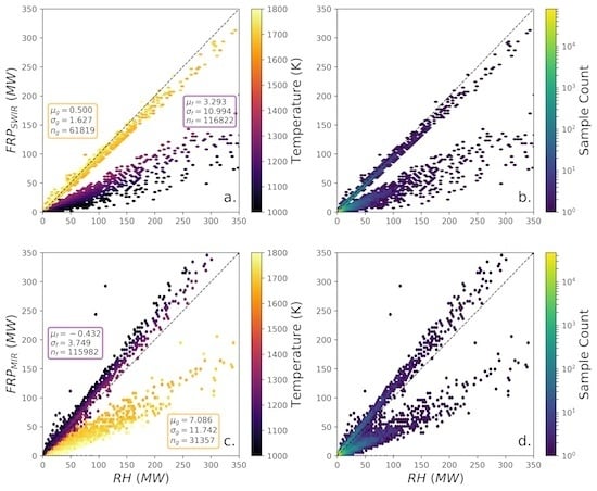
Figure 5 shows that the majority of NightFire algorithm hotspots with effective temperatures exceeding 1600 K are associated with well-known flaring locations in the Middle East and North/West Africa, whilst those with retrieved temperatures lower than 1600 K are mostly associated with seasonal biomass burning (landscape fires). For the hotter (i.e., mainly gas flare) hotspots, the mean of the NightFire-derived temperatures is 1785 (± 147) K, whilst that for the cooler (i.e., mainly landscape fire) hotspots is 1118 (± 180) K. Whilst there is an apparent bimodal temperature distribution between biomass and non-biomass combustion activity [20], some probable gas flare locations show retrieved combustion temperatures < 1600 K and some biomass burning regions ≥ 1600 K (which is realistic on occasion, see [27]), though these represent less than 5% of each dataset. We compared the NightFire RH outputs at hotspots pixels calculated using these hotspot effective temperatures to our FRPSWIR retrievals derived via the SWIR-Radiance method and also the FRPMIR retrievals from the MIR-Radiance method (Figure 6). To ensure an appropriate evaluation, we further restrict the dataset to only those hotspots with estimated sub-pixel fire temperatures within each algorithm's suitable temperature range (i.e., 1600–2200 K and 650–1300 K for the SWIR- and MIR-Radiance methods respectively). Figure 6 shows the SWIR-Radiance analysis for 61,819 individual combustion events that resulted in NightFire-estimated sub-pixel hotspot effective temperatures of between 1600 K and 2200 K (i.e., assumed to be primarily gas flares) and for 116,822 combustion events between 650 K and 1300 K (i.e., assumed to be primarily landscape fires). For the hotspots assumed to be landscape fires, FRPSWIR is low-biased compared to the NightFire RH measure (µ = 3.3 MW), with a high degree of scatter ( = 11 MW). This is as expected from the simulations shown in Figure 1 and Figure 4, since SWIR based FRP retrievals are unsuitable for hotspots in the biomass burning temperature range. Conversely, for the hotspots assumed to be gas flares, FRPSWIR and RH show excellent agreement, with a very small bias ( = 0.5 MW) and low scatter ( = 1.6 MW), again as expected since the Figure 1 and Figure 4 simulations indicate that for hotpots at effective temperature of between 1600 K and 2200 K the SWIR-Radiance method of FRP retrieval provides an unbiased estimate of radiative heat output, very close to that provided by the NightFire algorithm via fitting of the Planck function to the observed multispectral radiances. The single wavelength SWIR-Radiance method thus appears very appropriate for FRP assessment at gas flares but not at landscape fires, due to the latter’s lower effective combustion temperature. The existing MIR-Radiance method should remain in use at landscape fires and as demonstrated in Figure 6c,d there is excellent agreement between FRPMIR and the NightFire RH measure (bias () of just −0.4 MW and a low scatter () of 3.8 MW; based on 115,982 samples). By contrast, for the assumed gas flares (i.e., those hotspots with 1600 ≤ T ≤ 2200 K), Figure 6c shows FRPMIR to be low-biased compared to the NightFire RH measure (µ = 7.1 MW), with high degree of scatter (σ = 11.7 MW). The number of samples used (31,357) for the MIR assessment differs from the SWIR analysis due to the differing hotspot sensitivities of the two channels (resulting in the fact that some gas flares show no isolatable MIR signal). As expected from the theoretical analysis of Section 2.1, the MIR-Radiance method is less appropriate for determining the FRP of higher temperature features such as gas flares and even a simple correction applied to correct the bias between the FRPMIR and RH measure would not reduce the high degree of scatter seen in Figure 6c, primarily because of the temperature dependent non-linearity demonstrated in Figure 1 between the ratio of the total radiant emittance and the MIR spectral radiance.
3. Multi-Sensor Evaluation of SWIR-Radiance Method Derived FRP
Section 2 has provided strong evidence of the suitability of the SWIR-Radiance method for gas flare FRP determination, albeit in this case only at night and using moderate spatial resolution data (VIIRS M-band (1.6 µm)). Many more EO imaging systems provide potentially suitable observations in the SWIR, including by day and this section analyses the performance of such observing systems when used with the FRPSWIR approach.
3.1. Sensors and Data
To facilitate the most extensive multi-sensor evaluation, daytime data was used as certain spaceborne instruments (e.g., MODIS) turn off their SWIR measurement capabilities at night. By day, terrestrial gas flares can be very easily detected with higher spatial resolution imagers such as Landsat OLI [51] but given water’s very low spectral reflectance at SWIR wavelengths we found it best to use maritime flares as here we found even moderate spatial resolution imagers such as MODIS were able to deliver isolatable flare-emitted SWIR spectral radiances. When we extended this to even coarser spatial resolution sensors, such as Meteosat SEVIRI operated from geostationary orbit, we found only the largest of gas flares delivered analysable SWIR signals, so these sensors were not included in our comparisons due to the very small sample size. We therefore focus on Landsat-8 OLI, MODIS and VIIRS.
Landsat-8 OLI images the Earth morning and night at a spatial resolution of 30 m in the VIS through SWIR spectral region (12-bit quantisation) and is very capable of detecting pixels containing actively burning landscape fires [52] as well as maritime and terrestrial gas flares [51]. MODIS is carried on both the Aqua and Terra satellites [15], providing morning, afternoon and night-time observations across 36 spectral channels with 12-bit quantisation at the following nadir spatial resolutions: 250 m (red and NIR channels), 500 m (remaining VIS to SWIR channels) and 1 km (TIR channels). We focus on the 500 m SWIR channels for flare detection and characterisation, whereas for active fires the 1 km MIR and LWIR channel data are most commonly used [16,53]. VIIRS, carried on-board the Suomi-NPP satellite, was already used in Section 3 and the sensor acquires 12-bit early afternoon and night-time imagery in five 375 m spatial resolution channels (VIS through LWIR), referred to as I-bands (operated by day only) and sixteen 750 m spatial resolution channels (VIS through LWIR), referred to as M-bands. Having already demonstrated the effectiveness of VIIRS M-Band data for gas flare FRP in Section 3, here we focus on the higher spatial resolution I-band data, with pixel areas four times smaller than the M-band data and thus an ability to detect flares whose FRP is approximately four times lower (minimum detectable FRP being inversely proportional to pixel area; [25]). VIIRS I-band data has previously been employed to detect landscape fires that are significantly smaller than those detectable in the M-Bands [22,54]. Unlike all other data used in this comparison, VIIRS data is pre-processed on-board the Suomi-NPP satellite using a spatial aggregation procedure to minimise changing pixel area across the swath. In the centre third of the scan, signals from three separate measurement pixels are averaged to produce the output pixel signal, moving out towards the scan edge such averaging is reduced to two pixels and then removed entirely. Full details of this spatial averaging are included in [22].
The study region (latitude 5.05–6.35°S, longitude 11.0–11.9°E) is located over the Cabinda oil fields. This is a large and productive oil reserve off the Angolan coast, with limited capacity for natural gas processing and hence significant gas flaring. A mostly cloud-free Landsat OLI daytime image was obtained at 09:22 UTC on 27 April 2015 and the associated standard terrain corrected L1T product retrieved from the USGS Earth Explorer (http://earthexplorer.usgs.gov/). Approximately 3.5 h after the OLI acquisition (at 12:58 UTC) the same area was imaged close to nadir by VIIRS, again with limited cloud cover. At this near-central location in the VIIRS swath, three native resolution VIIRS pixels are aggregated to form the final recorded 375 m pixel I-band signal and we obtained the VIIRS sensor data record (SDR) product for this overpass from the NOAA CLASS database (http://www.class.ncdc.noaa.gov/). Finally, mostly cloud-free image of the same area was obtained around 24 h prior to the VIIRS overpass by Aqua MODIS and was downloaded from the NASA LAADSWeb data store (https://ladsweb.nascom.nasa.gov/) in L1B format, again with the study site is located close to nadir and thus without impact from the MODIS bow-tie effect [55].
3.2. Gas Flare Detection, Characterisation and Comparison
Initial inspection of the daytime OLI imagery indicated that various non-flaring maritime features were present that could be flagged as flares if an overly simple SWIR channel signal threshold were used for flare identification. Therefore, a slightly more complex multi-spectral approach was employed, based on signals in OLI bands 6 (SWIR; 1.6 µm) and 11 (LWIR; 12 µm, coming from the Thermal Infrared Sensor instrument (TIRS) also present on Landsat-8 along with OLI). The signal threshold employed for both channels was the study region mean plus four standard deviations, with these calculated from non-flare pixels contained within the region of interest (to exclude potential flare pixels the threshold process was applied twice: the first iteration removing obvious flare pixels and the second iteration providing a flare free estimates of the background signal mean and standard deviation). No additional cloud masking was necessary, since cloud-contaminated pixels had signals very similar to that of the water in the LWIR band and so were removed via the LWIR data masking procedure). Manual checks confirmed our OLI-based detection approach proved well suited for this limited inter-sensor comparison, though it would require more sophistication for more widespread application (e.g., [50]) and a total of 221 Landsat OLI pixels were identified as having elevated radiances caused by gas flaring, clustered into 10 distinct individual spatial features (Figure 7).
For MODIS, we first applied a 307 K brightness temperature threshold applied to the LWIR (Band 32, 12 µm) data to discriminate between cloudy and cloud free pixels, cloud being more numerous here than in the other datasets. The resulting cloud mask was buffered by two pixels to ensure exclusion of optically thin cloud and cloud peripheries. Furthermore, unlike the OLI flare pixel assessments (and the VIIRS assessments discussed next) which employed the 1.6 µm SWIR channel for flare detection, for MODIS we used the 2.2 µm (band 7) channel because broken detectors in the Aqua MODIS 1.6 µm channel lead to dropped lines and data loss [56]. Detection of flare pixels was based on exactly the same SWIR channel statistical thresholding approach as employed with OLI but now applied to the 2.2 µm data and this identified a total of 22 MODIS flare pixels, clustered into 12 spatially distinct gas flaring locations.
Finally, the flare pixel detection procedure was enacted on the VIIRS I-band data, based once again on the same thresholding approach to the instruments SWIR channel data, in this case applied to VIIRS-I3 (1.6 µm). A total of 32 VIIRS-I3 Band pixels with raised signals indicative of high temperature targets were found, clustered into 16 spatially distinct flaring locations.
The disparity in the number of flare clusters detected across the three different sensors (10 distinct regions of flaring activity detected by OLI, 16 by VIIRS and 12 by MODIS) maybe somewhat influenced by the greatly differing sensor spatial resolutions and perhaps the slightly different detection approaches employed but appears primarily a result of differing gas flaring characteristics being present at the time of each overpass. The 10 flares detected by Landsat are, however, also detected by MODIS and VIIRS, so it was this common set that was used for the intercomparison of gas flare FRP. To extract the signals of all the pixels common to the matching flares, an approach was employed where 0.02° × 0.02° bounding boxes centred on the mean geographic positions of each of the ten OLI-detected flare clusters were defined. The latitude and longitude of each OLI, VIIRS and MODIS hotspot pixel were then evaluated to determine their parent cluster. The 221 OLI pixels covering flare activity were found to be associated with 21 VIIRS pixels and 16 MODIS pixels, spread across the 10 flaring sites and the total FRP for each flare was computed from the recorded top of atmosphere spectral radiances. We did not apply an adjustment for non-unitary transmittance of the atmosphere (like [23]), because within the SWIR atmospheric windows centred on 1.6 µm and 2.2 µm, as discussed in Section 2.3, absorption due to atmospheric gases including water vapour is calculated to be very similar and to not exceed 10% of the upwelling radiance and with very little dependence on atmospheric moisture variations [48]. Mean background spectral radiance values, , were computed from the non-flaring (and cloud-free) regions surrounding each flare for use in the derivation of FRP. In the case of OLI, a 125 × 125 pixel region centred on the mean flare location was used, whereas with VIIRS and MODIS a 10 × 10 pixel region was used. The computed background radiances were subtracted from the radiances of each flare pixel and the FRP calculated using Equation (5), with the appropriate FRP coefficient and with VIIRS and MODIS pixel areas () calculated from the sensor scan angle using methods discussed in [20] and [55]. An assumed 900 m2 pixel area was used for OLI. Individual per-pixel FRP values were then summed to provide the total flare FRP, shown in Figure 8.
Figure 8a indicates a good agreement between the per-flare FRP values derived using the SWIR-radiance method with VIIRS I-band (375 m pixels, 1.6 µm waveband) and MODIS (500 m pixels, 2.2 µm waveband). The relationship between the two independent FRP measures follows approximately a 1:1 line, with a bias () of 2.2 MW and a scatter () of 8.2 MW. This indicates relatively good agreement between the FRP data of the two sensors, which have pixel areas around an order of magnitude different and where FRP has been derived using two different SWIR wavebands (1.6 and 2.2 µm). The significant scatter could be contributed by many factors, for example changes in flaring behaviour caused by wind or flare gas supply variations; different viewing angles resulting in changes to the observed cross sectional areas of the flare and in turn the observed SWIR radiances; potentially different soot absorption coefficients at the two wavelengths used and different flame depths at the observed viewing directions [57], as well as the aforementioned differences in SWIR atmospheric transmission.
In contrast to the strong agreement between the VIIRS- and MODIS-derived FRP’s shown in Figure 8a, the OLI-derived FRP values show a marked dissimilarity to those from the other two sensors (Figure 8b,c respectively). The higher spatial resolution OLI data delivers FRP values far lower than the moderate spatial resolution sensors, all below 5 MW compared to up to 55 MW from MODIS and VIIRS. Further investigation shows this low bias stems from the fact that each gas flare cluster contains at least one pixel whose signal exceeds the nominal detector range (LMAX) of the OLI 1.6 µm channel, specified as 71.3 W m−2 sr−1 µm−1 [58], though none reach the stated saturation level (LSAT) of 96 W m−2 sr−1 µm−1 [58]. In [52] it is shown that when strongly emitting hotspots cause the OLI-measured per-pixel signal to exceed LMAX, spurious values can result (even in cases where the signal remains much lower than LSAT). However, the good agreement between VIIRS and MODIS shown in Figure 8a suggests strong performance from the approach when applied to these significantly more moderate spatial resolution sensors, whose SWIR channel detectors remain well within their nominal dynamic range over the flare targets (because the flares represent a far smaller proportion of the pixels ground FOV than with OLI). A suitable approach for extracting valid FRP estimates from gas flares using OLI data is a Planck fitting approach using channels whose signals remain in the nominal detector range and this is demonstrated in Appendix A1.
4. Summary and Conclusions
Satellite Earth observation has been used to quantify the thermal radiant power output of industrial gas flares and because these measures correlate to flare CO2 production figures they can be used to track the success of global gas flaring emissions reduction efforts. We have evaluated for the first time the efficacy of single channel satellite Earth observation methods of fire radiative power (FRP) retrieval from flaring sites. FRP-retrieval approaches like the MIR radiance method, originally designed for use at sites of landscape fires [1,2], can operate without the constraints of ancillary data requirements and are insensitive to inter-channel spatial mis-registration effects. They are also usable with older sensors with fewer spectral bands—such as ATSR—whose data are inappropriate for use with multi-spectral FRP retrieval algorithms. However, we find the MIR radiance approach inappropriate for use at industrial gas flaring locations, due to the higher combustion temperatures involved that invalidate certain of the methods assumptions. We demonstrate however, that an adaptation of the approach to use SWIR rather than MIR radiance data does prove effective for flare FRP retrieval, because the 4th order power law approximation to the Planck function that underlies the MIR radiance method becomes more valid at shorter wavelengths as emitter temperatures increase. A major advantage of this so-called ‘SWIR radiance’ method over other FRP retrieval approaches is that it requires no detailed knowledge of flare target temperature, yet removing this requirement only introduces a maximum error of ±13.6% when using SWIR observations at 1.6 µm and ±6.3% at 2.2 µm (assuming the flares lie within a temperature range of 1600–2200 K). Narrowing the assumed range to 1700–1800 K, within which many flare effective temperatures appear to lie, reduces uncertainties to the very minor figures of −2.1 ± 1.9% (at 1.6 µm) and 5.8 ± 0.3% (at 2.2 µm) respectively. The fixed 1810 K flare temperature assumption employed in the initial NightFire 1.6 µm single channel algorithm of [20] is expected to perform slightly less effectively than the approach presented here (when considering the same channel), with an expected mean error of −3.7 ± 1.9% over the 1700–1800 K interval and up to ±15% across the wider assumed flare temperature range. The more recent single channel NightFire algorithm [23] improves on this, provided that the nearby higher-intensity flare from which the effective temperature estimate is obtained is a good approximation to the temperature of the lower intensity flare under analysis. If not, this approach can lead to errors in retrieved FRP of up to 24%.
We have applied this new SWIR-Radiance approach to data from the moderate spatial resolution VIIRS imager and compared results to those generated using the NightFire algorithm of [20] and to FRPs derived using the new algorithm applied to MODIS. Analysing two months of FRP data over Africa and the Middle East, along with a more targeted assessment over the Cabinda oilfield of Angola, our intercomparisons provide strong evidence that the single waveband SWIR radiance method delivers accurate gas flare FRPs when applied to moderate resolution imaging systems such as VIIRS and MODIS, just as the MIR radiance method does for landscape fires [1,2].
Spectral emissions from gas flares peak in the SWIR, meaning that our single waveband, SWIR-based approach can provide a more extensive assessment of FRP from flaring activities from spaceborne EO compared to methods that rely on flare detectability in shorter (or longer) wavelength channels. Requiring the flare signal to be resolvable in only a single SWIR band also maximises the range of EO sensors to which the technique can be applied and in the future, we anticipate deriving gas flare FRP from the (Advanced) Along Track Scanning Radiometer (ATSR) series of sensors that possessed a night-time-operating SWIR band, enabling the assessment of global gas flaring reduction efforts starting in 1991 to be assessed [59] and providing a possible constraint on the contributions to anthropogenic carbon emissions from this source.
Acknowledgments
VIIRS NightFire data were obtained via the NOAA National Geophysical Data Centre. VIIRS data were obtained via the NOAA Comprehensive Large Array-data Stewardship System. MODIS data were obtained via the NASA Level 1 and Atmosphere Archive and Distribution System. Landsat data were obtained via the USGS EarthExplorer system. This work was supported by the Natural Environment Research Council through the National Centre for Earth Observation (NCEO).
Author Contributions
Daniel Fisher and Martin J. Wooster conceived and designed the experiments; Daniel Fisher performed the experiments; Daniel Fisher analysed the data; Daniel Fisher and Martin J. Wooster wrote the paper.
Conflicts of Interest
The authors declare no conflict of interest.
Appendix A1. Medium vs. Moderate Resolution FRP comparison
Section 3 showed that Landsat OLI fails to measure SWIR radiances accurately over intensely emitting sub-pixel hot targets such as gas flares, and thus cannot be used with the SWIR radiance approach to provide data for the validation of results from more moderate spatial resolution sensors. However, such validations are still desirable to perform, and so an alternative approach for OLI-based FRP retrieval was developed, based on the type of Planck function fitting used within the VIIRS NightFire algorithm of [20]. Planck function fitting has been used before with nighttime OLI data, for example to identify regions of flaming and smouldering combustion in peat and forest fires by [60], and similar approaches were used with airborne data of fires by [61]. The primary advantage is that the fit can avoid use of OLI bands whose radiances are higher than LMAX, enabling the exploitation of only accurately recorded signals. The disadvantage is that the technique is confined largely to use of nighttime OLI data, because by day solar insolation dominates the observed spectral signals at the shorter OLI wavebands, at least over high albedo surfaces. Nevertheless, use of this technique enables us to reliably include high spatial resolution OLI data in multi-sensor FRP intercomparisons, and thus provides a means of validating the FRP retrievals made by the moderate spatial resolution imagers with the new SWIR radiance approach.
Figure A1.
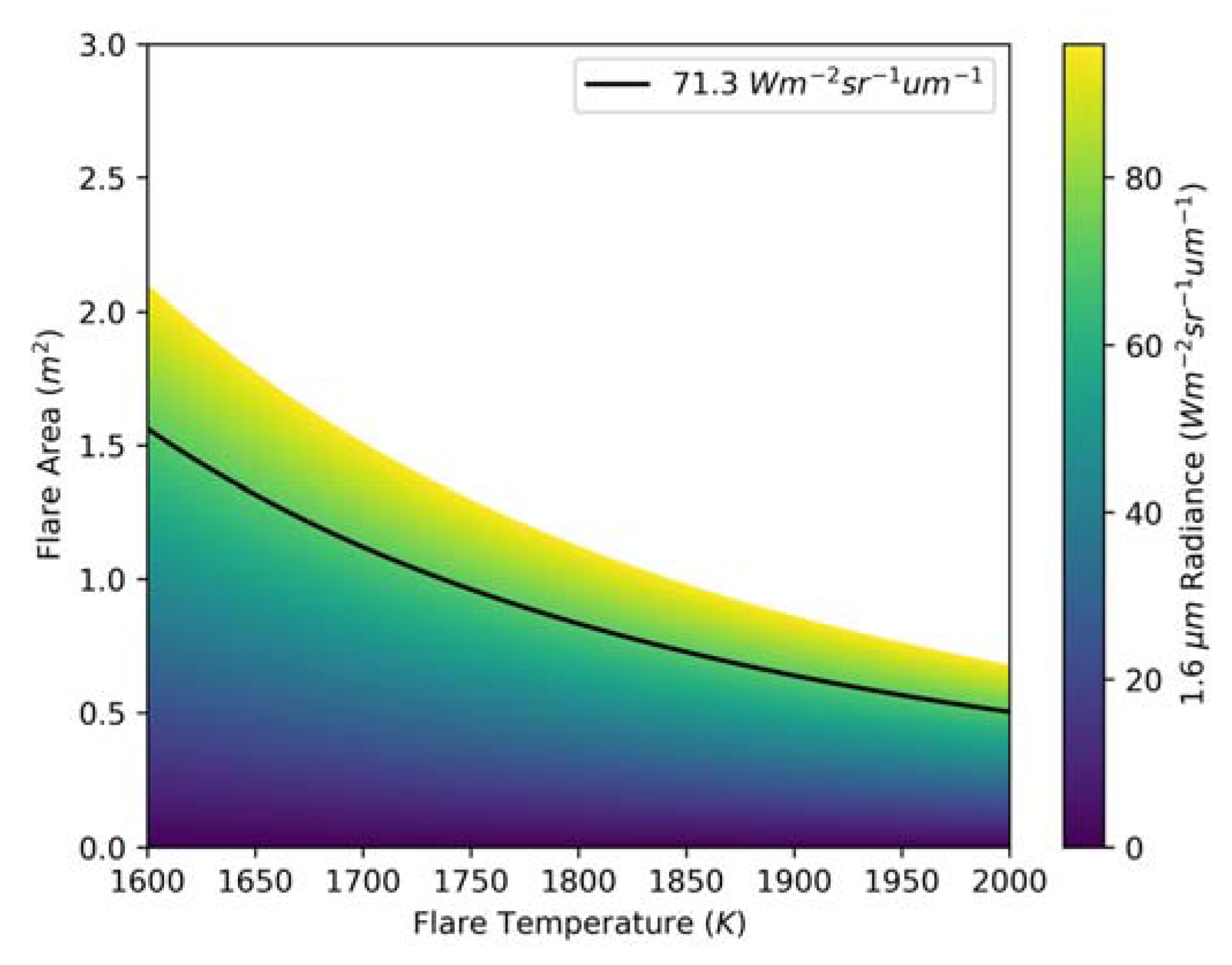
Modelled spectral radiances for high temperature events, calculated for a 1.6 µm wavelength and for various hotspot effective temperatures and sub-pixel areas and assuming a pixel area of 900 m2 representing the Landsat OLI sensor. The black line indicates the OLI 1.6 µm channel nominal detector range (LMAX) spectral radiance cut-off and LSAT cut-off is the interface between the white and coloured regions.
Figure A1.
Modelled spectral radiances for high temperature events, calculated for a 1.6 µm wavelength and for various hotspot effective temperatures and sub-pixel areas and assuming a pixel area of 900 m2 representing the Landsat OLI sensor. The black line indicates the OLI 1.6 µm channel nominal detector range (LMAX) spectral radiance cut-off and LSAT cut-off is the interface between the white and coloured regions.
A1.1. Planck Fit Derived FRP from Landsat OLI
As already noted, the radiant intensity of industrial gas flaring typically leads to saturation or problematic near-saturation in the SWIR channels of Landsat OLI (See Figure A1), but the OLI VIS/NIR channels show data over gas flares that is highly detectable and very easy to discriminate from the near-zero level background signals at night. We exploit this here to apply a Plank Function fitting approach to nighttime OLI data recorded over gas flares in the visible and NIR channels (Bands 2 to 5; blue through NIR), bypassing the problems found in the OLI SWIR channels in Section 3. Similar to the NightFire approach of [23], we do not apply any adjustments to the data to counteract atmospheric effects, and rather than fitting the Planck function on a pixel-by-pixel basis as is case with the NightFire algorithm, we instead use the mean spectral radiances computed from all pixels relevant to each entire flare hotspot in order to remove the effect of any inter-channel spatial misregistration that may potentially degrade the quality of the Planck fitting results [37]. This is similar to the approach adopted for applying the Dozier [40] dual-band approach to data from the BIRD Hotspot Recognition Sensor (HSRS, [43]), and to data of volcanic targets by [62]. The spatial domain of each flare in the OLI data is identified through a single threshold applied to the band 6 (1.6 µm) imagery, as discussed in the following Section, but these SWIR band data are not used in the actual fit. A prior temperature of 2000 K and flare fractional area of 1% are used to initialise the Planck function fitting process. Following fitting of the Planck function to the OLI-measured mean spectral radiances recoded across the VIS to NIR spectral channels, the total flare FRP is calculated using Stefan’s constant, (W m-2 K-4), with the derived hotspot effective temperature (, K) and area , the area (m2) of the summed OLI pixels making up the flare, and , a scaling factor (unitless), also derived from the Planck fitting process, representing the flares factional area:
A1.2. Evaluation of OLI Planck Fit FRP against VIIRS M-Band SWIR-Radiance FRP
To apply this approach to Landsat OLI, a total of 21 OLI nighttime scenes (path: 32, row: 205) were obtained from the Earth Explorer data center (http://earthexplorer.usgs.gov/) for a region of interest located over Southern Iraq (latitude range: [31.2N, 30.0N], longitude range: [47.2E, 48.2E]; see Figure 4 and Figure A1). This area contains several super-giant oil fields with significant production capabilities and associated high magnitude gas flaring. Scenes were acquired between October 2014 and October 2015, with each ascending node acquisition occurring at approximately 18:40 UTC. The VIIRS M-band data products temporally closest to each Landsat scene and where the flare was observed in the near nadir aggregation zone were used (retrieved from the NOAA CLASS data store; http://www.class.ncdc.noaa.gov/), these being collected 2 days prior to the Landsat-8 overpasses, at approximately 22:00 UTC in the descending node of the Suomi-NPP satellite.
Figure A2.
Cloud-free OLI Band 6 (1.6 µm) nighttime image of the Southern Iraq study region, obtained at 18:40 on 28th January 2015. Flare hotspots used in the FRP intercomparison with VIIRS are easily seen, with the flare mask described in Appendix A1.2 applied to the image and the SWIR signal converted to spectral radiance (logarithmic colour scale applied). See Figure 5 location 2 for the geographic location of the ROI.

OLI flare pixels were again derived through masking of the B6 (1.6 µm channel) data, at the level of the image mean plus four standard deviations, and this mask used to extract spectral radiances from all OLI channels used in the Planck function fit (OLI Bands 2 to 6). Flare pixels were spatially clustered into 31 individual flare hotspots, defined through examination of the data of Figure A2, which allowed extraction of flare centres along with signals in a 0.02° × 0.02° bounding box. Any channel showing clustered pixels whose signal exceeded the LMAX value specified in [58] was not used in the Planck function fit for that flare. The resulting dataset comprised a set of OLI-derived FRPs for comparison against the FRPs generated from the much coarser spatial resolution VIIRS observations input into the SWIR radiance method, with VIIRS flare pixels identified using the same masking procedure and used to extract the VIIRS SWIR signals at each of the 31 flare hotspots identified by OLI. Occasionally no flare was detectable in the temporally closest VIIRS scene and the next available scene had to be used instead. Usually this was the result of cloud obscuration, but occasionally occurred in cloud-free scenes, presumably because of a temporary shutdown of flaring.
Matching VIIRS- and OLI-derived flare FRPs are compared in Figure A3 (a), and compared to Figure 8 (b) we see a very much reduced bias (mean of -7.5 MW, median 1.7 MW) between the VIIRS SWIR-Radiance derived FRPs and those generated by the Planck fit and the OLI data. This improved agreement is a result of us not now using the SWIR band OLI data in the FRP retrieval from OLI, since this was noted to recording incorrect signals over flare targets, as discussed in Section 3.2.
Figure A3.
Intercomparison of VIIRS M-Band derived gas flare FRP calculated using the SWIR-Radiance method with that derived from OLI using (a) the Planck fit approach, and (b) the SWIR-Radiance method. Insets show the statistics for all data points, with 31 flare hotspots used measured across 21 collocated OLI and VIIRS images—providing a total of total of 391 comparisons.
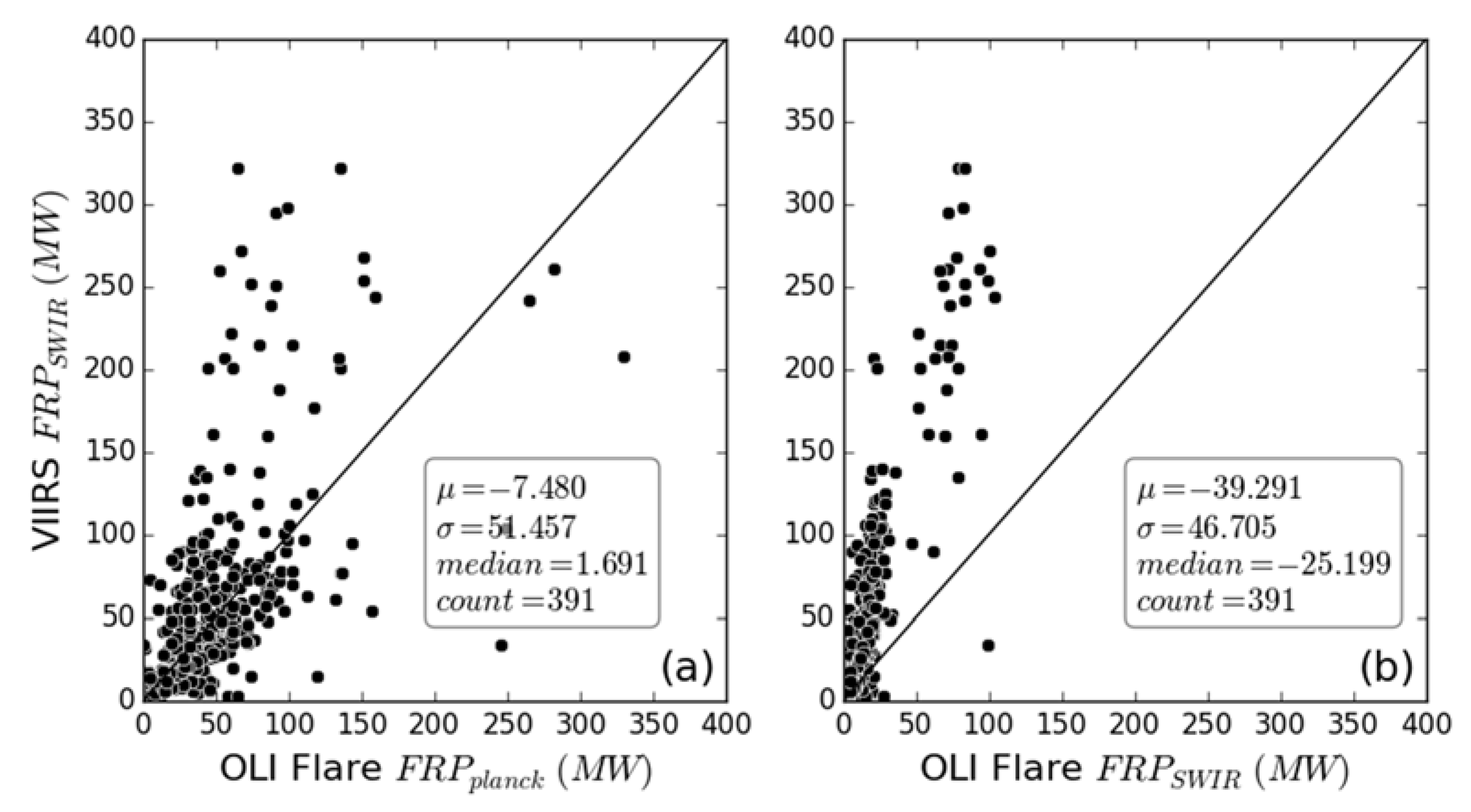
The much-improved agreement seen in Figure A3 (a) between FRPs derived from OLI (via the Plank-fit method) and VIIRS (derived via the SWIR radiance approach) still, however, contains a substantial degree of variance. At least some of this variation is very likely to be caused by real changes in the flaring activity between the Landsat-8 and Suomi-NPP overpasses, for example alterations in the number of individual stacks where gas is being flared off (each flare ‘hotspot’ in these Iraq flares is a set of individual flare stacks). However, for flares with an FRP exceeding ~ 100 MW, there does seem to be an apparent underestimation when compared to VIIRS. Further investigation of this will be the subject of future study.
References
- Wooster, M.J.; Zhukov, B.; Oertel, D. Fire radiative energy for quantitative study of biomass burning: Derivation from the BIRD experimental satellite and comparison to MODIS fire products. Remote Sens. Environ. 2003, 86, 83–107. [Google Scholar] [CrossRef]
- Wooster, M.J.; Roberts, G.; Perry, G.L.W.; Kaufman, Y.J. Retrieval of biomass combustion rates and totals from fire radiative power observations: FRP derivation and calibration relationships between biomass consumption and fire radiative energy release. J. Geophys. Res. Atmos. 2005, 110. [Google Scholar] [CrossRef]
- Ichoku, C.; Kaufman, Y.J. A method to derive smoke emission rates from MODIS fire radiative energy measurements. IEEE Trans. Geosci. Remote Sens. 2005, 43, 2636–2649. [Google Scholar] [CrossRef]
- Kaufman, Y.J.; Remer, L.; Ottmar, R.; Ward, D.; Li, R.R.; Kleidman, R.; Fraser, R.S.; Flynn, L.; McDougal, D.; Shelton, G. Relationship between remotely sensed fire intensity and rate of emission of smoke: SCAR-C experiment. In Global Biomass Burning; MIT Press: Cambridge, MA, USA, 1996; pp. 685–696. [Google Scholar]
- Kaufman, Y.J.; Kleidman, R.G.; King, M.D. SCAR-B fires in the tropics: Properties and remote sensing from EOS-MODIS. J. Geophys. Res. Atmos. 1998, 103, 31955–31968. [Google Scholar] [CrossRef]
- Kremens, R.L.; Dickinson, M.B.; Bova, A.S. Radiant flux density, energy density and fuel consumption in mixed-oak forest surface fires. Int. J. Wildland Fire 2012, 21, 722–730. [Google Scholar] [CrossRef]
- Roy, D.P.; Jin, Y.; Lewis, P.E.; Justice, C.O. Prototyping a global algorithm for systematic fire-affected area mapping using MODIS time series data. Remote Sens. Environ. 2005, 97, 137–162. [Google Scholar] [CrossRef]
- Roy, D.P.; Boschetti, L.; Justice, C.O.; Ju, J. The collection 5 MODIS burned area product—Global evaluation by comparison with the MODIS active fire product. Remote Sens. Environ. 2008, 112, 3690–3707. [Google Scholar] [CrossRef]
- Wooster, M.J.; Roberts, G.; Perry, G.L.; Kaufman, Y.J. Retrieval of biomass combustion rates and totals from fire radiative power observations: Application to Southern Africa using geostationary SEVIRI imagery. J. Geophys. Res. Atmos. 2005, 110. [Google Scholar] [CrossRef]
- Roberts, G.J.; Wooster, M.J. Fire detection and fire characterization over Africa using Meteosat SEVIRI. IEEE Trans. Geosci. Remote Sens. 2008, 46, 1200–1218. [Google Scholar] [CrossRef]
- Freeborn, P.H.; Wooster, M.J.; Hao, W.M.; Ryan, C.A.; Nordgren, B.L.; Baker, S.P.; Ichoku, C. Relationships between energy release, fuel mass loss and trace gas and aerosol emissions during laboratory biomass fires. J. Geophys. Res. Atmos. 2008, 113. [Google Scholar] [CrossRef]
- Ellicott, E.; Vermote, E.; Giglio, L.; Roberts, G. Estimating biomass consumed from fire using MODIS FRE. Geophys. Res. Lett. 2009, 36. [Google Scholar] [CrossRef]
- Kaiser, J.W.; Heil, A.; Andreae, M.O.; Benedetti, A.; Chubarova, N.; Jones, L.; Morcrette, J.-J.; Razinger, M.; Schultz, M.G.; Suttie, M. Biomass burning emissions estimated with a global fire assimilation system based on observed fire radiative power. Biogeosciences 2012, 9, 527–554. [Google Scholar] [CrossRef] [Green Version]
- Ichoku, C.; Ellison, L. Global top-down smoke-aerosol emissions estimation using satellite fire radiative power measurements. Atmos. Chem. Phys. 2014, 14, 6643–6667. [Google Scholar] [CrossRef] [Green Version]
- Kaufman, Y.J.; Herring, D.D.; Ranson, K.J.; Collatz, G.J. Earth Observing System AM1 mission to earth. IEEE Trans. Geosci. Remote Sens. 1998, 36, 1045–1055. [Google Scholar] [CrossRef]
- Giglio, L.; Descloitres, J.; Justice, C.O.; Kaufman, Y.J. An enhanced contextual fire detection algorithm for MODIS. Remote Sens. Environ. 2003, 87, 273–282. [Google Scholar] [CrossRef]
- Giglio, L.; Csiszar, I.; Restás, Á.; Morisette, J.T.; Schroeder, W.; Morton, D.; Justice, C.O. Active fire detection and characterization with the advanced spaceborne thermal emission and reflection radiometer (ASTER). Remote Sens. Environ. 2008, 112, 3055–3063. [Google Scholar] [CrossRef]
- Xu, W.; Wooster, M.J.; Roberts, G.; Freeborn, P. New GOES imager algorithms for cloud and active fire detection and fire radiative power assessment across North, South and Central America. Remote Sens. Environ. 2010, 114, 1876–1895. [Google Scholar] [CrossRef]
- Wooster, M.J.; Xu, W.; Nightingale, T. Sentinel-3 SLSTR active fire detection and FRP product: Pre-launch algorithm development and performance evaluation using MODIS and ASTER datasets. Remote Sens. Environ. 2012, 120, 236–254. [Google Scholar] [CrossRef]
- Elvidge, C.D.; Zhizhin, M.; Hsu, F.-C.; Baugh, K.E. VIIRS nightfire: Satellite pyrometry at night. Remote Sens. 2013, 5, 4423–4449. [Google Scholar] [CrossRef]
- Peterson, D.; Wang, J.; Ichoku, C.; Hyer, E.; Ambrosia, V. A sub-pixel-based calculation of fire radiative power from MODIS observations: 1: Algorithm development and initial assessment. Remote Sens. Environ. 2013, 129, 262–279. [Google Scholar] [CrossRef]
- Schroeder, W.; Oliva, P.; Giglio, L.; Csiszar, I.A. The New VIIRS 375 m active fire detection data product: Algorithm description and initial assessment. Remote Sens. Environ. 2014, 143, 85–96. [Google Scholar] [CrossRef]
- Elvidge, C.D.; Zhizhin, M.; Baugh, K.; Hsu, F.-C.; Ghosh, T. Methods for global survey of natural gas flaring from visible infrared imaging radiometer suite data. Energies 2015, 9, 14. [Google Scholar] [CrossRef]
- Giglio, L.; Schroeder, W.; Justice, C.O. The collection 6 MODIS active fire detection algorithm and fire products. Remote Sens. Environ. 2016, 178, 31–41. [Google Scholar] [CrossRef]
- Wooster, M.J.; Roberts, G.; Freeborn, P.H.; Xu, W.; Govaerts, Y.; Beeby, R.; He, J.; Lattanzio, A.; Fisher, D.; Mullen, R. LSA SAF Meteosat FRP products–Part 1: Algorithms, product contents and analysis. Atmos. Chem. Phys. 2015, 15, 13217–13239. [Google Scholar] [CrossRef]
- Dennison, P.E.; Charoensiri, K.; Roberts, D.A.; Peterson, S.H.; Green, R.O. Wildfire temperature and land cover modeling using hyperspectral data. Remote Sens. Environ. 2006, 100, 212–222. [Google Scholar] [CrossRef]
- Lobert, J.M.; Warnatz, J. Emissions from the combustion process in vegetation. Fire Environ. 1993, 13, 15–37. [Google Scholar]
- Boulet, P.; Parent, G.; Acem, Z.; Kaiss, A.; Billaud, Y.; Porterie, B.; Pizzo, Y.; Picard, C. Experimental investigation of radiation emitted by optically thin to optically thick wildland flames. J. Combust. 2011, 2011. [Google Scholar] [CrossRef]
- Malvos, H.; Raj, P.K. Details of 35 m diameter LNG fire tests conducted in Montoir, France in 1987 and analysis of fire spectral and other data. In Proceedings of the AIChE Winter Conference, Orlando, FL, USA, 26 April 2006. [Google Scholar]
- Zhang, X.; Scheving, B.; Shoghli, B.; Zygarlicke, C.; Wocken, C. Quantifying gas flaring CH4 consumption using VIIRS. Remote Sens. 2015, 7, 9529–9541. [Google Scholar] [CrossRef]
- Haus, R.; Wilkinson, R.; Heland, J.; Schäfer, K. Remote sensing of gas emissions on natural gas flares. Pure Appl. Opt. 1998, 7, 853. [Google Scholar] [CrossRef]
- Ismail, O.S.; Umukoro, G.E. Global impact of gas flaring. Energy Power Eng. 2012, 4. [Google Scholar] [CrossRef]
- The World Bank Global Gas Flaring Reduction Partnership (GGFR)—Improving Energy Efficiency & Mitigating Impact on Climate Change; World Bank: Washington, DC, USA, 2011.
- Johnson, M.R.; Coderre, A.R. Compositions and greenhouse gas emission factors of flared and vented gas in the Western Canadian Sedimentary Basin. J. Air Waste Manag. Assoc. 2012, 62, 992–1002. [Google Scholar] [CrossRef] [PubMed]
- Field, R.A.; Soltis, J.; Murphy, S. Air quality concerns of unconventional oil and natural gas production. Environ. Sci. Process. Impacts 2014, 16, 954–969. [Google Scholar] [CrossRef] [PubMed]
- Smith, D.; Mutlow, C.; Delderfield, J.; Watkins, B.; Mason, G. ATSR infrared radiometric calibration and in-orbit performance. Remote Sens. Environ. 2012, 116, 4–16. [Google Scholar] [CrossRef]
- Shephard, M.W.; Kennelly, E.J. Effect of band-to-band coregistration on fire property retrievals. IEEE Trans. Geosci. Remote Sens. 2003, 41, 2648–2661. [Google Scholar] [CrossRef]
- Giglio, L.; Kendall, J.D. Application of the Dozier retrieval to wildfire characterization: A sensitivity analysis. Remote Sens. Environ. 2001, 77, 34–49. [Google Scholar] [CrossRef]
- Giglio, L.; Schroeder, W. A global feasibility assessment of the bi-spectral fire temperature and area retrieval using MODIS data. Remote Sens. Environ. 2014, 152, 166–173. [Google Scholar] [CrossRef]
- Dozier, J. A method for satellite identification of surface temperature fields of subpixel resolution. Remote Sens. Environ. 1981, 11, 221–229. [Google Scholar] [CrossRef]
- Freeborn, P.H.; Wooster, M.J.; Roy, D.P.; Cochrane, M.A. Quantification of MODIS fire radiative power (FRP) measurement uncertainty for use in satellite-based active fire characterization and biomass burning estimation. Geophys. Res. Lett. 2014, 41, 1988–1994. [Google Scholar] [CrossRef]
- Gaydon, A.G.; Wolfhard, H.G. Flames, Their Structure, Radiation and Temperature; Halsted Press: New York, NY, USA, 1979. [Google Scholar]
- Zhukov, B.; Lorenz, E.; Oertel, D.; Wooster, M.; Roberts, G. Spaceborne detection and characterization of fires during the bi-spectral infrared detection (BIRD) experimental small satellite mission (2001–2004). Remote Sens. Environ. 2006, 100, 29–51. [Google Scholar] [CrossRef]
- Polivka, T.N.; Wang, J.; Ellison, L.T.; Hyer, E.J.; Ichoku, C.M. Improving Nocturnal Fire Detection With the VIIRS Day–Night Band. IEEE Trans. Geosci. Remote Sens. 2016, 54, 5503–5519. [Google Scholar] [CrossRef]
- Reed, R.J. Combustion Handbook; North American Manufacturing Co.: Cleveland, OH, USA, 1986; Volume 1. [Google Scholar]
- Leifer, I.; Lehr, W.J.; Simecek-Beatty, D.; Bradley, E.; Clark, R.; Dennison, P.; Hu, Y.; Matheson, S.; Jones, C.E.; Holt, B. State of the art satellite and airborne marine oil spill remote sensing: Application to the BP Deepwater Horizon oil spill. Remote Sens. Environ. 2012, 124, 185–209. [Google Scholar] [CrossRef]
- Casadio, S.; Arino, O.; Serpe, D. Gas flaring monitoring from space using the ATSR instrument series. Remote Sens. Environ. 2012, 116, 239–249. [Google Scholar] [CrossRef]
- Griffin, M.K.; Burke, H.-h.K. Compensation of hyperspectral data for atmospheric effects. Linc. Lab. J. 2003, 14, 29–54. [Google Scholar]
- Wooster, M.J.; Rothery, D.A. Thermal monitoring of Lascar Volcano, Chile, using infrared data from the along-track scanning radiometer: A 1992–1995 time series. Bull. Volcanol. 1997, 58, 566–579. [Google Scholar] [CrossRef]
- Wooster, M.J.; Rothery, D.A.; Sear, C.B.; Carlton, R.W.T. Monitoring the development of active lava domes using data from the ERS-1 along track scanning radiometer. Adv. Space Res. 1998, 21, 501–505. [Google Scholar] [CrossRef]
- Anejionu, O.C.D.; Blackburn, G.A.; Whyatt, J.D. Satellite survey of gas flares: Development and application of a Landsat-based technique in the Niger Delta. Int. J. Remote Sens. 2014, 35, 1900–1925. [Google Scholar] [CrossRef] [Green Version]
- Schroeder, W.; Oliva, P.; Giglio, L.; Quayle, B.; Lorenz, E.; Morelli, F. Active fire detection using Landsat-8/OLI data. Remote Sens. Environ. 2016, 185, 210–220. [Google Scholar] [CrossRef]
- Justice, C.O.; Giglio, L.; Korontzi, S.; Owens, J.; Morisette, J.T.; Roy, D.; Descloitres, J.; Alleaume, S.; Petitcolin, F.; Kaufman, Y. The MODIS fire products. Remote Sens. Environ. 2002, 83, 244–262. [Google Scholar] [CrossRef]
- Zhang, T.; Wooster, M.J.; Xu, W. Approaches for synergistically exploiting VIIRS I-and M-Band data in regional active fire detection and FRP assessment: A demonstration with respect to agricultural residue burning in Eastern China. Remote Sens. Environ. 2017, 198, 407–424. [Google Scholar] [CrossRef]
- Freeborn, P.H.; Wooster, M.J.; Roberts, G. Addressing the spatiotemporal sampling design of MODIS to provide estimates of the fire radiative energy emitted from Africa. Remote Sens. Environ. 2011, 115, 475–489. [Google Scholar] [CrossRef]
- Gladkova, I.; Grossberg, M.; Bonev, G.; Shahriar, F. A multiband statistical restoration of the Aqua MODIS 1.6 micron band. Int. Soc. Opt. Photon. 2011, 8048, 804819. [Google Scholar]
- Johnson, M.R.; Devillers, R.W.; Thomson, K.A. A generalized Sky-LOSA method to quantify soot/black carbon emission rates in atmospheric plumes of gas flares. Aerosol Sci. Technol. 2013, 47, 1017–1029. [Google Scholar] [CrossRef]
- Morfitt, R.; Barsi, J.; Levy, R.; Markham, B.; Micijevic, E.; Ong, L.; Scaramuzza, P.; Vanderwerff, K. Landsat-8 Operational Land Imager (OLI) radiometric performance on-orbit. Remote Sens. 2015, 7, 2208–2237. [Google Scholar] [CrossRef]
- Kaldany, R. Global gas flaring reduction initiative. In Oil, Gas and Chemicals World Bank Group, Marrakesh; World Bank: Washington, DC, USA, 2001. [Google Scholar]
- Elvidge, C.D.; Zhizhin, M.; Hsu, F.-C.; Baugh, K.; Khomarudin, M.R.; Vetrita, Y.; Sofan, P.; Hilman, D. Long-wave infrared identification of smoldering peat fires in Indonesia with nighttime Landsat data. Environ. Res. Lett. 2015, 10, 065002. [Google Scholar] [CrossRef]
- Amici, S.; Wooster, M.J.; Piscini, A. Multi-resolution spectral analysis of wildfire potassium emission signatures using laboratory, airborne and spaceborne remote sensing. Remote Sens. Environ. 2011, 115, 1811–1823. [Google Scholar] [CrossRef]
- Blackett, M.; Wooster, M.J. Evaluation of SWIR-based methods for quantifying active volcano radiant emissions using NASA EOS-ASTER data. Geomat. Nat. Hazards Risk 2011, 2, 51–78. [Google Scholar] [CrossRef]
Figure 1.
Ratios of radiant emittance (Stefan’s law) to spectral radiant emittance (Planck’s law) for different blackbody emitter temperatures at wavelengths commonly used by satellite Earth-imaging radiometers. A constant ratio at a given wavelength indicates that the Planck function can be well approximated by a 4th order power law over the defined temperature domain and that mapping from spectral radiance at that wavelength to total radiant emittance is possible using a constant term. Coloured regions represent combustion temperature domains common in landscape fires (in red) and in gas flares (in yellow). The dashed lines represent the wavelength used in the calculation of the spectral radiance. Note the log scale and the near constant ratio of total radiance to spectral radiance at MIR wavelengths for landscape fire combustion temperatures and similar behaviour at SWIR channels for gas flare combustion temperatures.

Figure 2.
Ratio of spectral radiances (Lλ) emitted at wavelengths at 1.6 µm and 3.7 µm for a range of hotspots having temperatures encompassing biomass burning, gas flaring and non-flaring industrial sites. The ratio is approximately monotonically increasing with increasing emitter temperature and thresholding can be used to effectively discriminate between different types of hotspots (e.g., at, respectively, a minimum and maximum value of around 2.5 and 5.5 W m−2 sr−1 µm−1. (W m−2 sr−1 µm−1)−1 for gas flaring at typically 1600–2200 K and 0 and 1.2 W m−2 sr−1 µm−1. (W m−2 sr−1 µm−1)−1 for landscape fires at typically 650–1300 K).
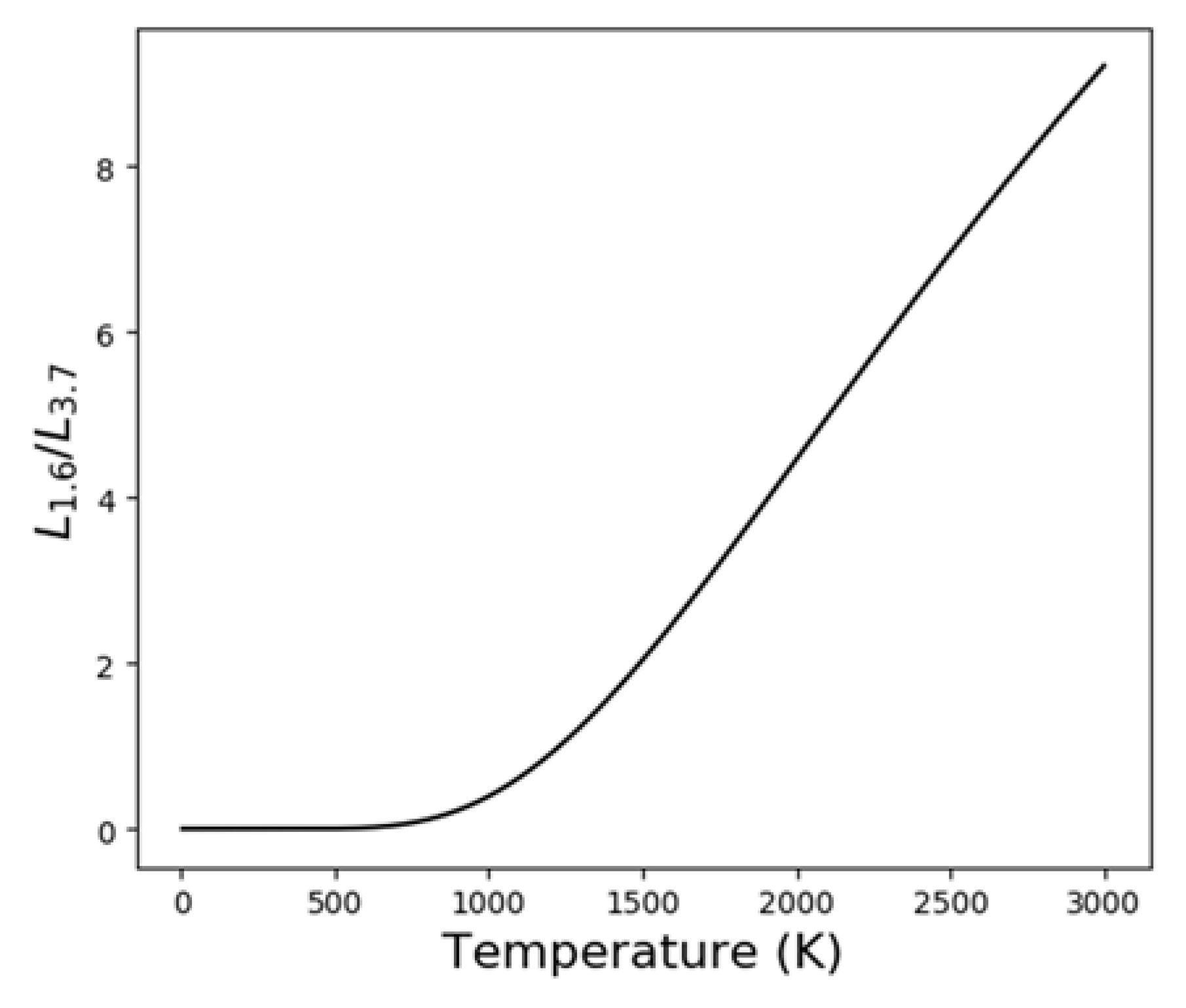
Figure 3.
Accuracy of SWIR-radiance method derived gas flare FRPs, as calculated using modelled flare scenarios of varying temperatures and with an assumed flare of area 100 m2 in a 1 km2 pixel. Plots show the ratio between FRP estimated using the modelled flare-emitted spectral radiance calculated via the Planck function and the SWIR radiance approach and that calculated directly from Stefan’s law (i.e., ‘truth’). Results are show for both (a) 2.2 µm and (b) 1.6 µm wavelengths and with the FRP coefficient used in the SWIR radiance method calculated for a range of different emitter temperatures. The x-axis plots the temperature parameter used to compute (see Equation (2)) in the FRP coefficient and the y-axis the modelled flare temperature. Black vertical lines represent the parameter temperature that gives the smallest maximum bias between the SWIR-radiance method-derived FRP and the true FRP, whilst dashed lines represent assumed flaring temperature range (1600 K to 2200 K) over which the biases are computed.
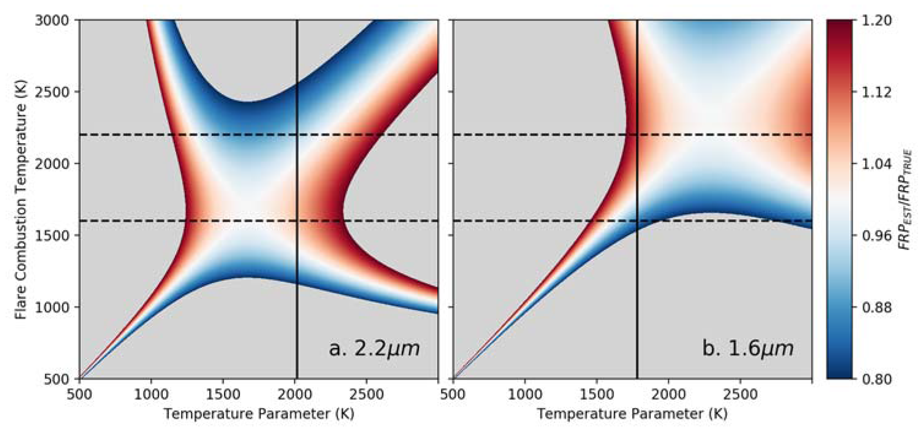
Figure 4.
Bias in retrieved FRP as a function of temperature, for single-waveband FRP retrievals made at 1.6, 2.2 and 4 µm respectively using optimised FRP coefficients for gas flaring temperatures of 1600–2200 K for the 1.6 and 2.2 µm channels and 650–1300 K landscape fire temperatures for the 4 µm channel. Temperatures minimising the maximum bias between the true and single-waveband retrieved FRP’s are 1782 K and 2016 K and for the 1.6 µm and 2.2 µm channels and 722 K and 1197 K for the 4 µm channel respectively. The single-band FRPs are calculated over the entire temperature range presented in the figure and compared to the true FRP for the same temperature calculated using Stefan’s law as follows: , providing the bias estimate for each wavelength and temperature (dashed lines). As with Figure 1 the coloured regions demark the combustion temperature domains for fires (red) and gas flares (yellow).

Figure 5.
Locations of VIIRS-detected hotspot pixels over Africa and the Middle-East within the VIIRS NightFire product [20], for (a) February 2015 and (b) September 2015, coloured by the effective subpixel hotspot temperature derived via the multi-spectral Planck function fitting approach described in [20]. Blue points indicate hotspot effective temperatures < 1600 K, whilst red points indicate ≥ 1600 K. The latter appear to be associated primarily with the well-known gas flaring regions in the Middle East, North Africa and West Africa, whereas the former are associated mainly with the locations of seasonal landscape biomass burning (e.g., matching those regions shown as burning in [10] at these times of year). Locations 1 and 2 shown in (a) represent the ROIs used in the analyses undertaken in Section 3 and in Appendix A1 respectively.
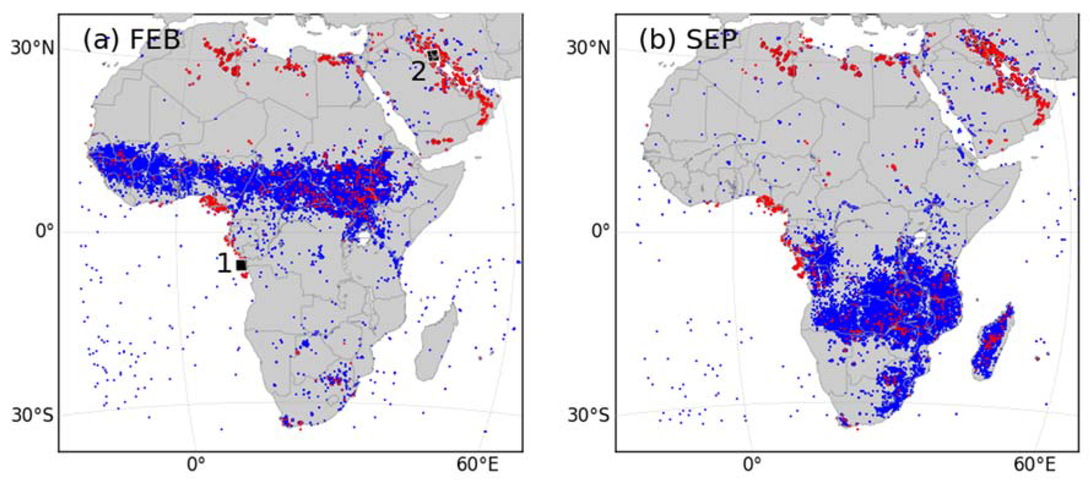
Figure 6.
Comparisons of night-time detected hotspot pixel radiative power outputs, calculated using either the SWIR-Radiance method developed herein (FRPSWIR; y-axis; plots (a) and (b)) or the MIR-Radiance method of [1,2] (FRPMIR; y-axis; plots (c) and (d)) and the radiative heat flux (RH, x-axis) measure based on application of the NightFire algorithm [20] using Plank function fitting. Data cover Africa and the Middle East in February and September 2015, as shown in Figure 5. The left-hand plots (a,c) represent the mean sub-pixel effective temperature of the hotspots present at each point on the scatterplot. The inset coloured boxes present statistics associated with the similarly coloured data points, with the subscript denoting assumed biomass burning (650 K ≤ T ≤ 1300 K) and denoting assumed gas flaring (1600 K ≤ T ≤ 2200 K). Right hand plots (b,d) show that each location on the scatterplot is typically composed of the results from multiple sub-pixel hotspot detections, particularly at lower radiative power output values.
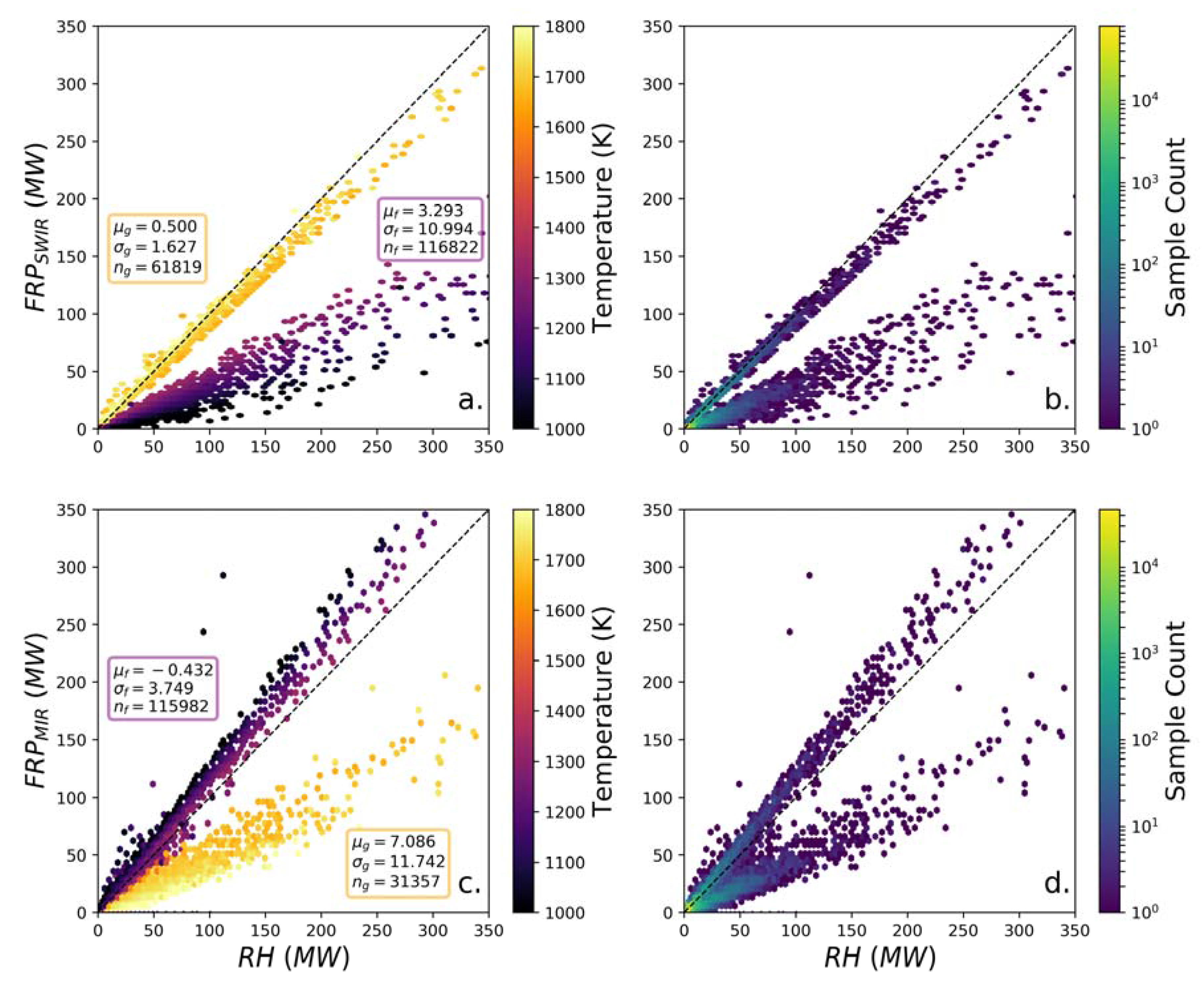
Figure 7.
Landsat OLI false colour composite (R: Band 6 G: Band 3 B: Band 2) covering the 10 locations of gas flaring detected by the Landsat-8 OLI sensor on the 27 April 2015 at 09:22 UTC.
Figure 7.
Landsat OLI false colour composite (R: Band 6 G: Band 3 B: Band 2) covering the 10 locations of gas flaring detected by the Landsat-8 OLI sensor on the 27 April 2015 at 09:22 UTC.

Figure 8.
Comparison of FRP totals derived for each flare, as calculated via the SWIR-Radiance method (Equation (4)) applied to Landsat-8, MODIS and VIIRS data of the ten flares identified by all systems in the study region of Figure 7. Plot (a) compares the FRP retrievals from MODIS and VIIRS, plot (b) those from Landsat OLI and VIIRS, and plot (c) those from Landsat OLI and MODIS.


Table 1.
The sensor specific FRP Coefficients used throughout the paper.
| Sensor | Band | FRP Coeff. |
|---|---|---|
| MODIS | B7 (2.13 µm) | 9.37 sr µm |
| VIIRS | M10 (1.61µm) | 7.32 sr µm |
| VIIRS | M13 (4.05 µm) | 23.14 sr µm |
| VIIRS | I3 (1.61 µm) | 7.32 sr µm |
| Landsat-OLI | B6 (1.61 µm) | 7.33 sr µm |
© 2018 by the authors. Licensee MDPI, Basel, Switzerland. This article is an open access article distributed under the terms and conditions of the Creative Commons Attribution (CC BY) license (http://creativecommons.org/licenses/by/4.0/).
Share and Cite
MDPI and ACS Style
Fisher, D.; Wooster, M.J. Shortwave IR Adaption of the Mid-Infrared Radiance Method of Fire Radiative Power (FRP) Retrieval for Assessing Industrial Gas Flaring Output. Remote Sens. 2018, 10, 305. https://doi.org/10.3390/rs10020305
AMA Style
Fisher D, Wooster MJ. Shortwave IR Adaption of the Mid-Infrared Radiance Method of Fire Radiative Power (FRP) Retrieval for Assessing Industrial Gas Flaring Output. Remote Sensing. 2018; 10(2):305. https://doi.org/10.3390/rs10020305
Chicago/Turabian StyleFisher, Daniel, and Martin J. Wooster. 2018. "Shortwave IR Adaption of the Mid-Infrared Radiance Method of Fire Radiative Power (FRP) Retrieval for Assessing Industrial Gas Flaring Output" Remote Sensing 10, no. 2: 305. https://doi.org/10.3390/rs10020305
Note that from the first issue of 2016, this journal uses article numbers instead of page numbers. See further details here.