Performance Assessment of Balloon-Borne Trace Gas Sounding with the Terahertz Channel of TELIS

 ,
,  ,
,
Abstract
:
1. Introduction
2. Overview of TELIS Measurements
2.1. Instrument
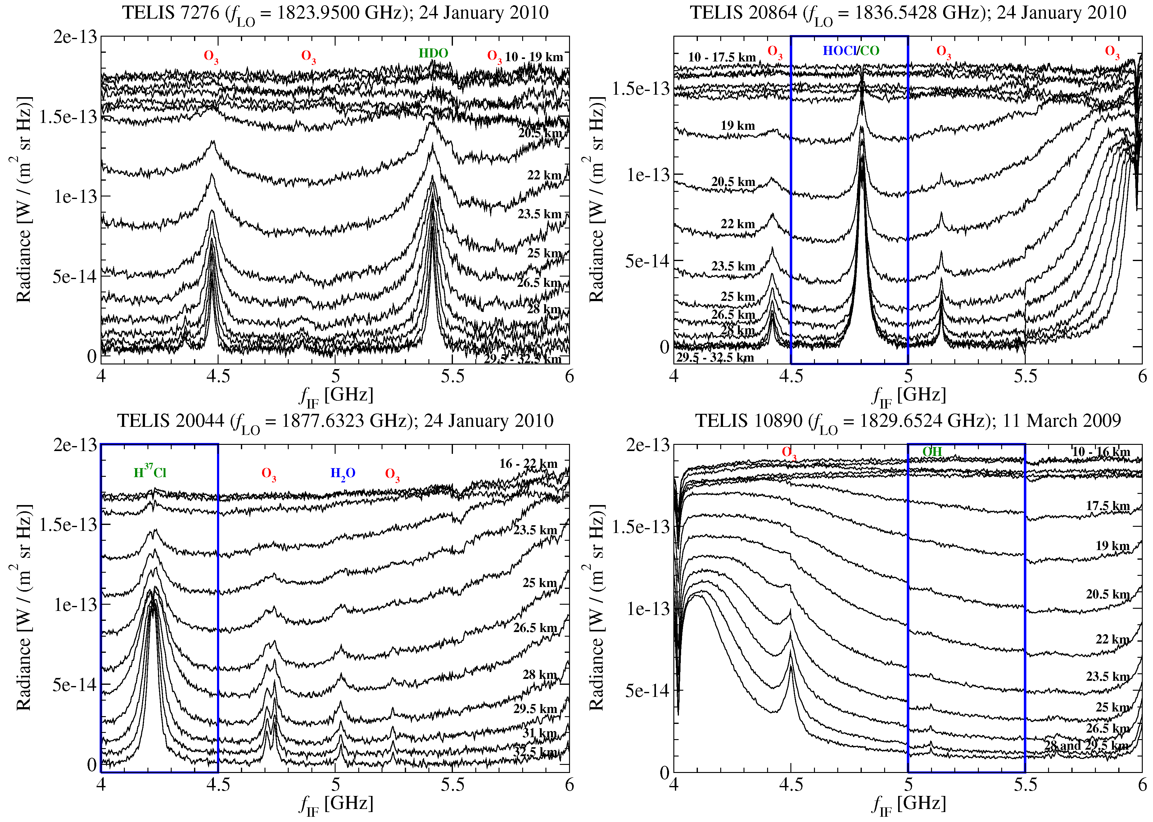
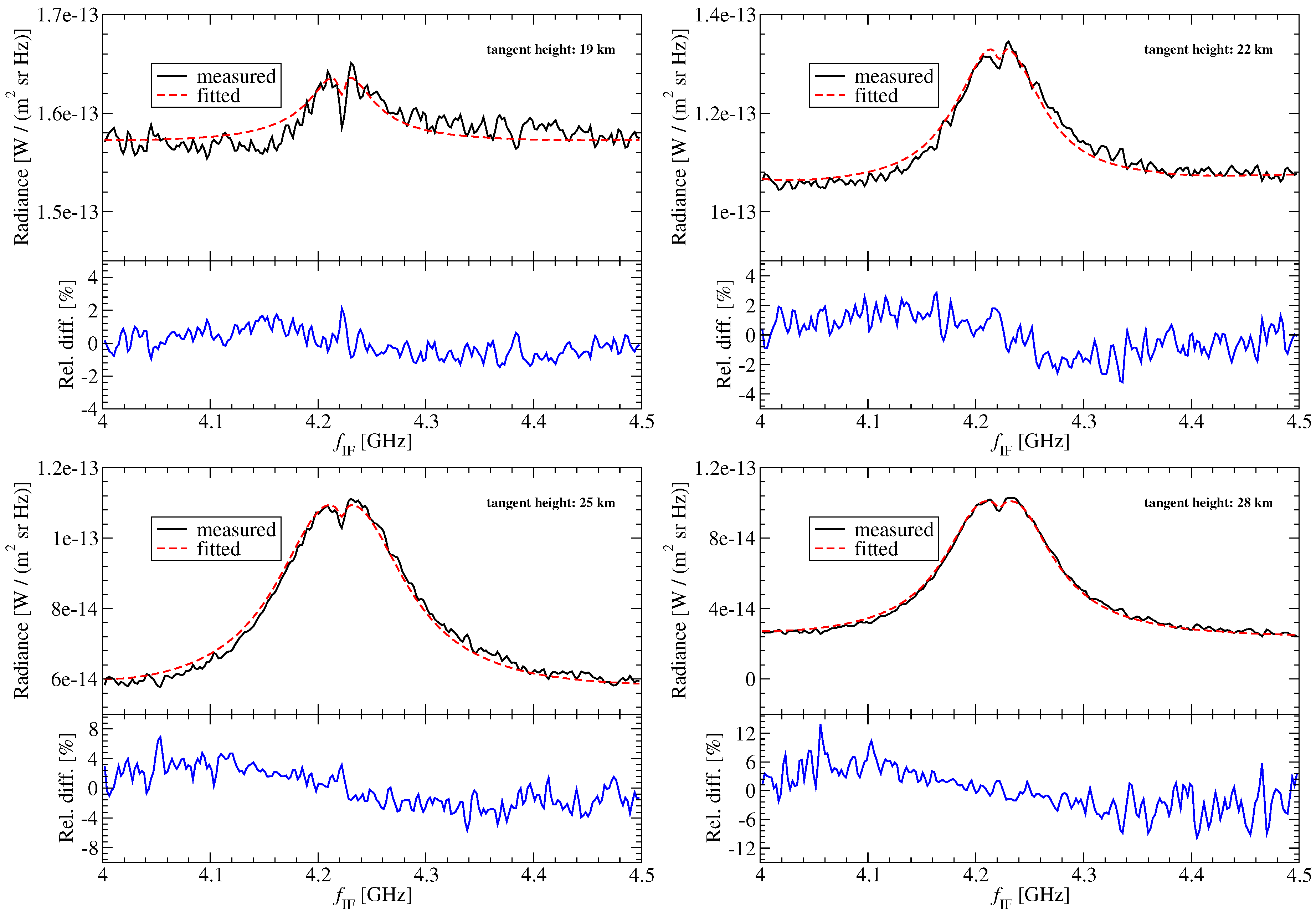
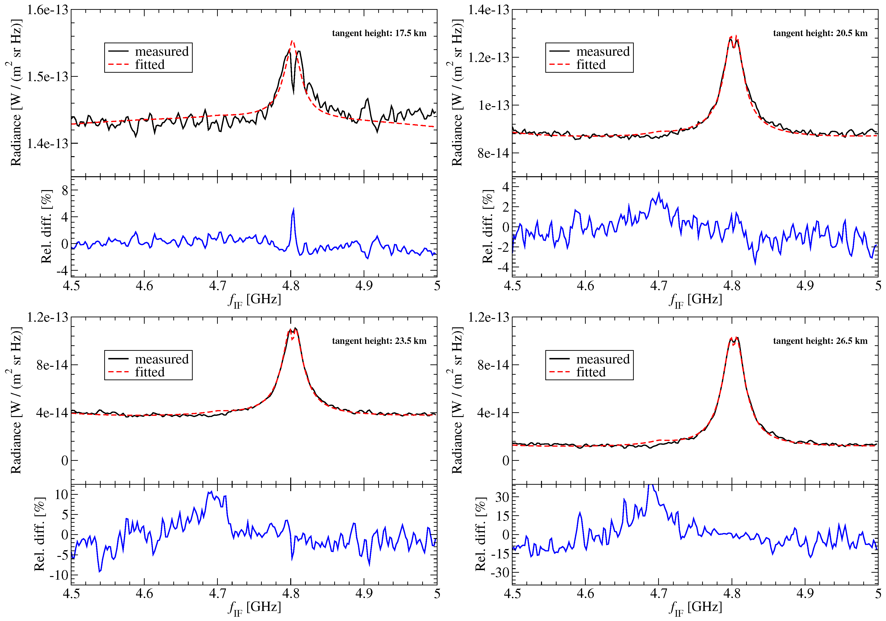
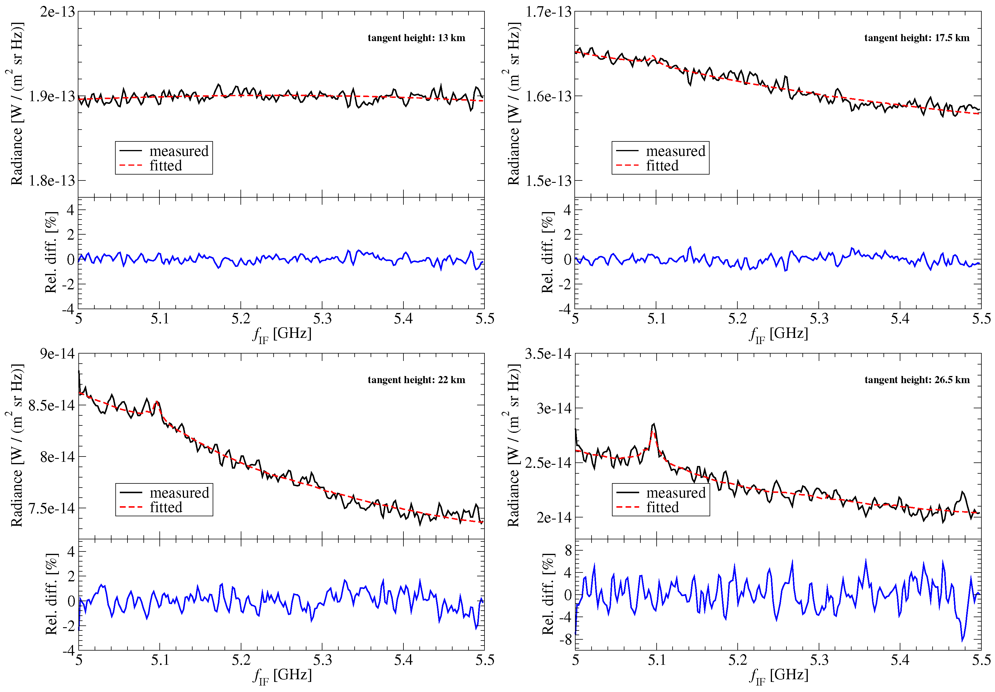
2.2. Limb Spectra
3. Retrieval Methodology
3.1. Inversion Framework
3.2. Retrieval Setup
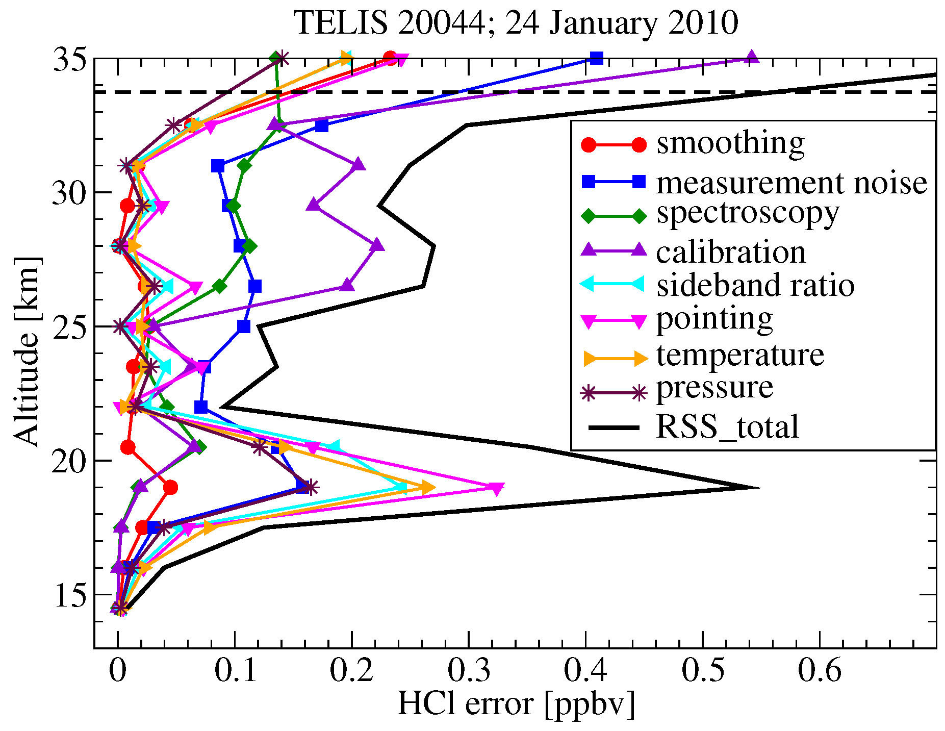
3.3. Error Characterization
3.4. Comparison Strategy
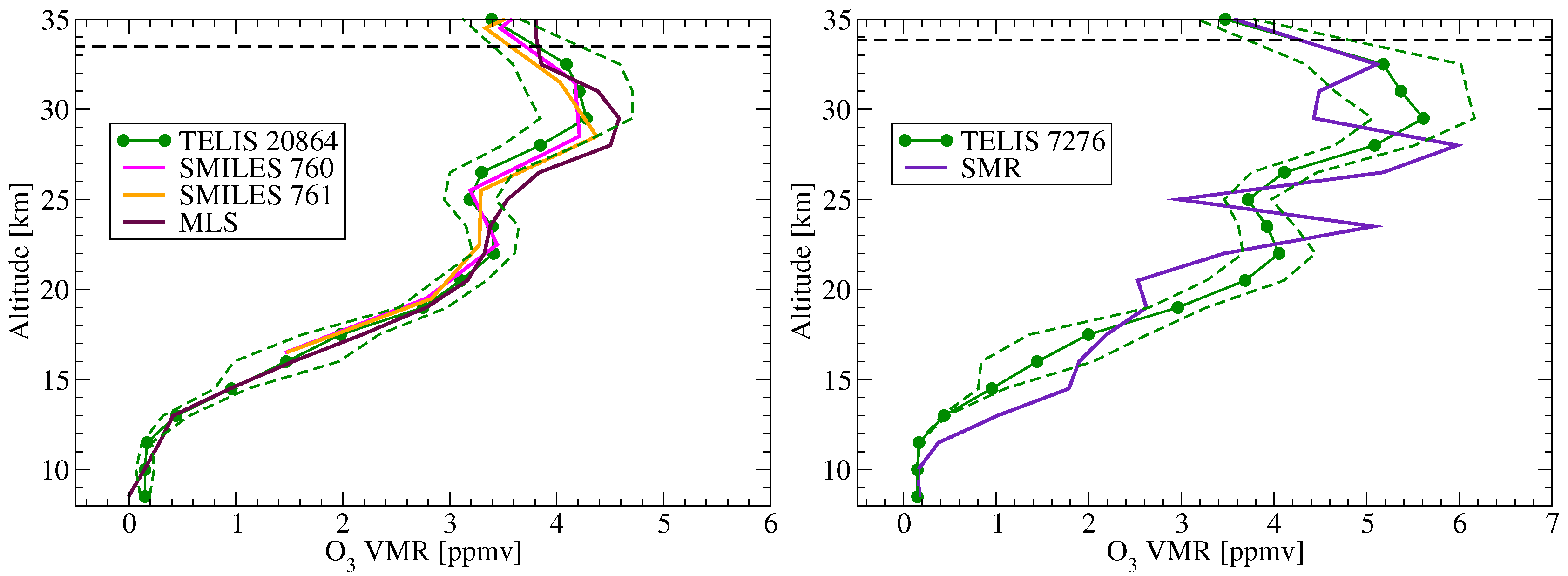
- SMILES: O3 profiles with measurement responses of no less than 0.8 and goodness of fit values of no more than 0.8 were used [32].
- MLS: O3 profiles with “Quality” fields greater than 0.6 and “Convergence” fields less than 0.8 [94], as well as HCl profiles with “Quality” fields greater than 1.2 and “Convergence” fields less than 1.05 [95], and CO profiles with “Quality” fields greater than 0.2 and “Convergence” fields less than 1.4 were used [93].
- SMR: O3 profiles with measurement responses greater than 0.75 and “QUALITY” flags equaling zero were used [83].
4. Results and Discussion
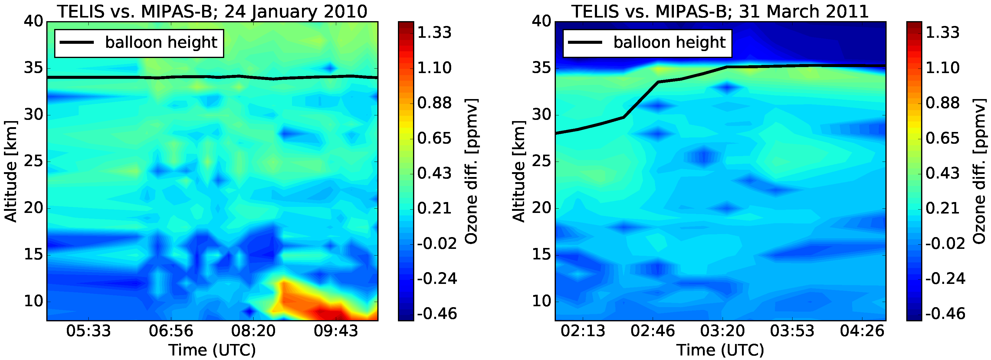
4.1. O3 Retrieval
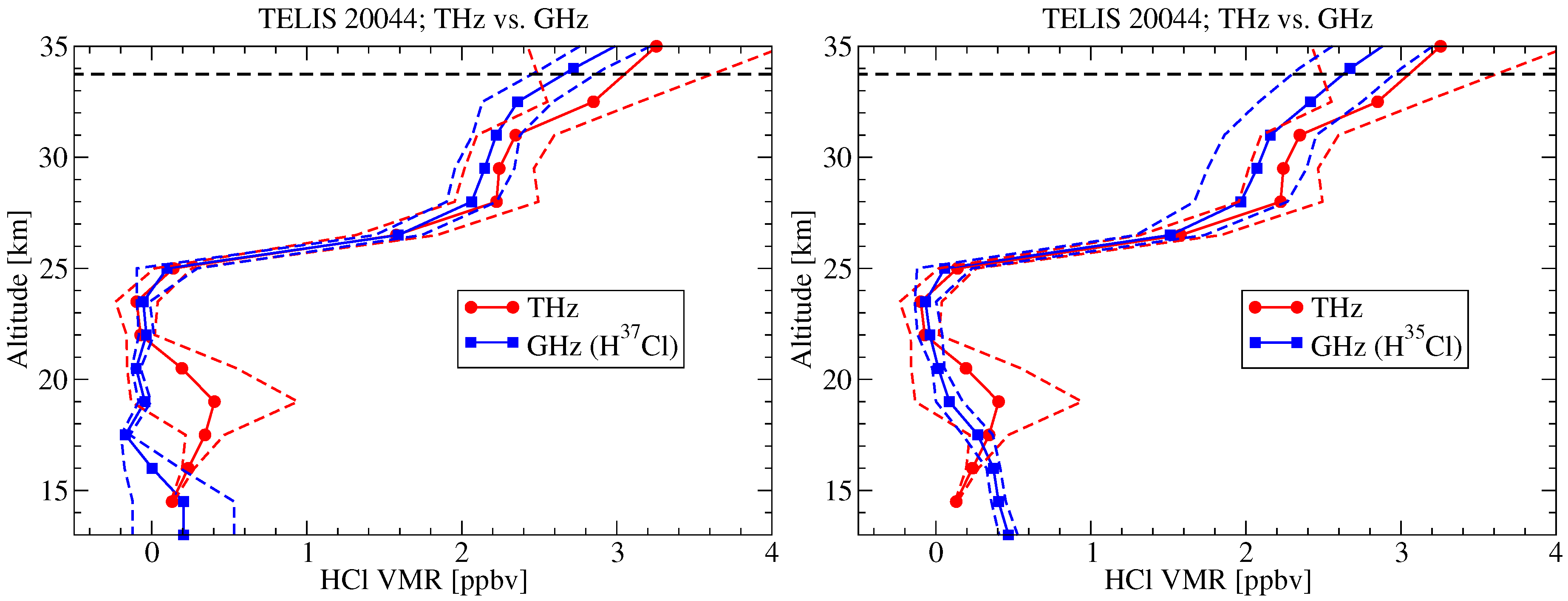
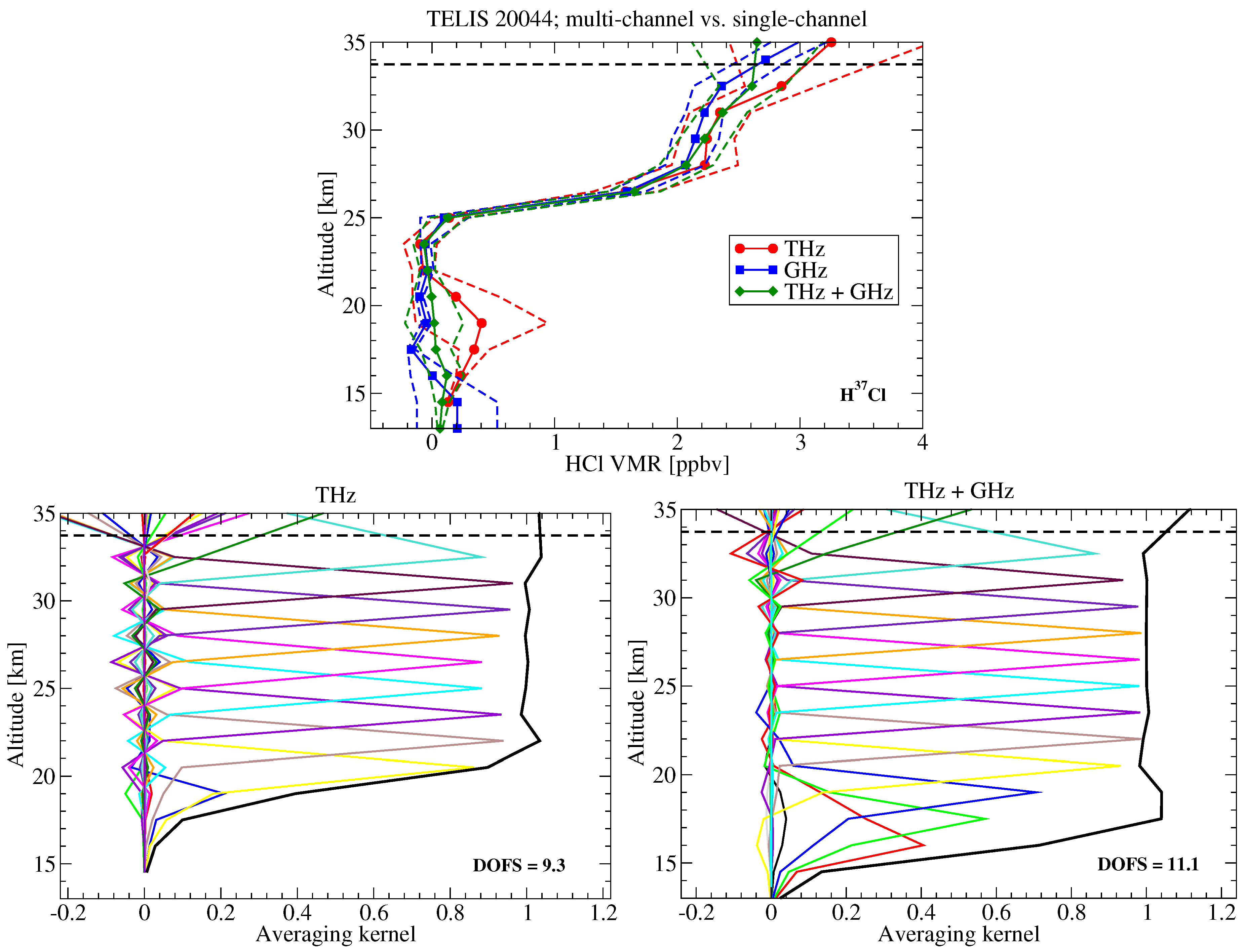
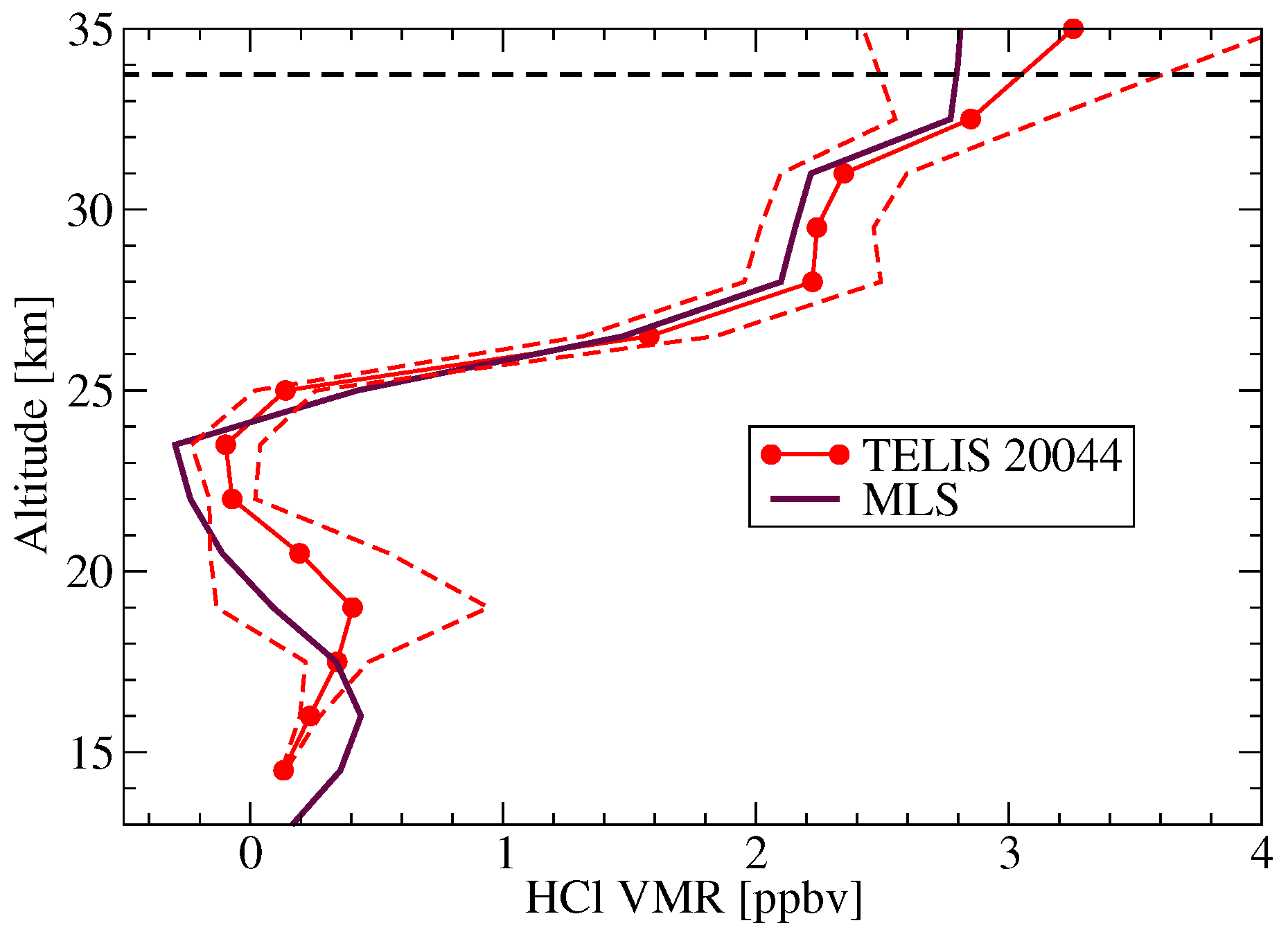
4.2. HCl Retrieval
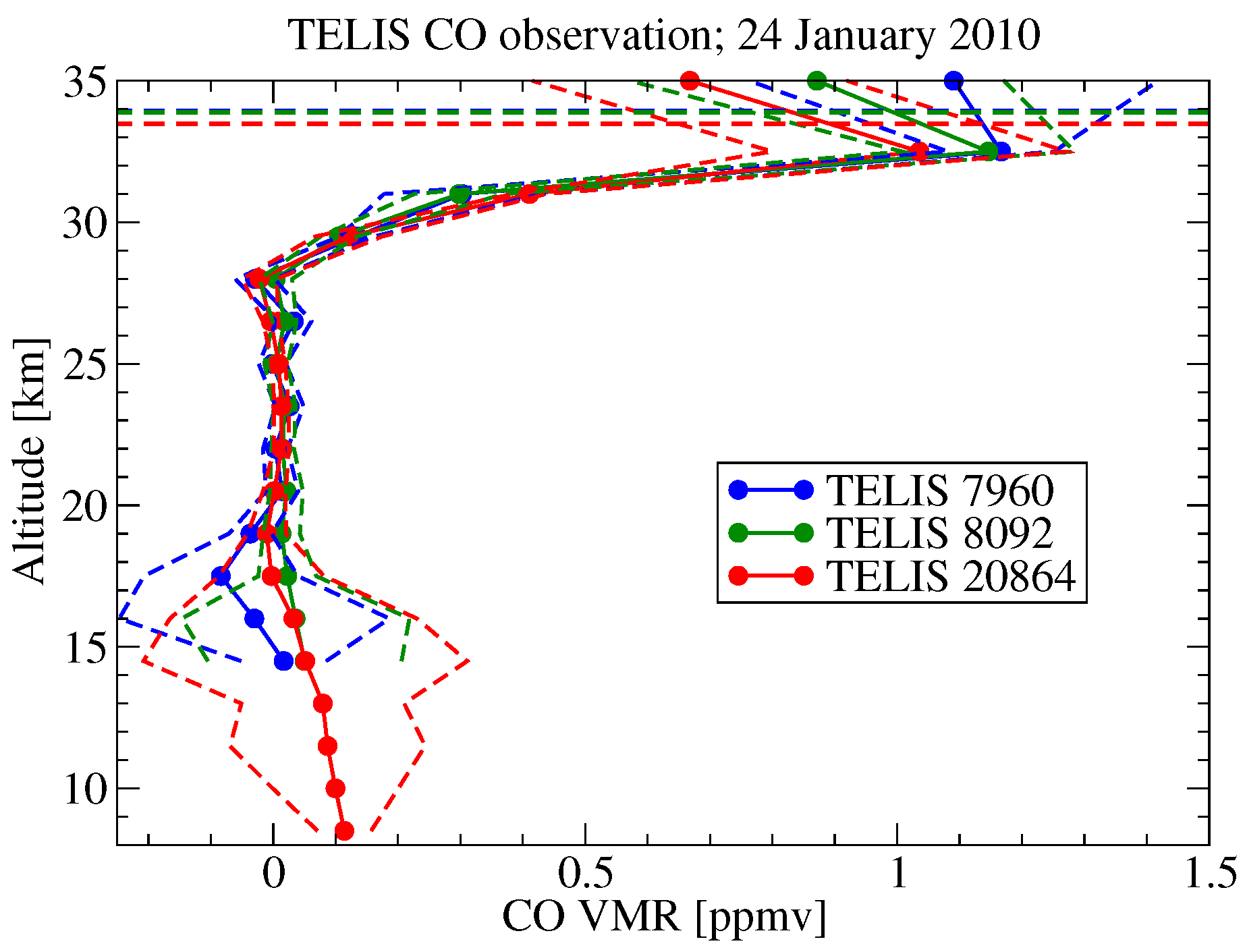
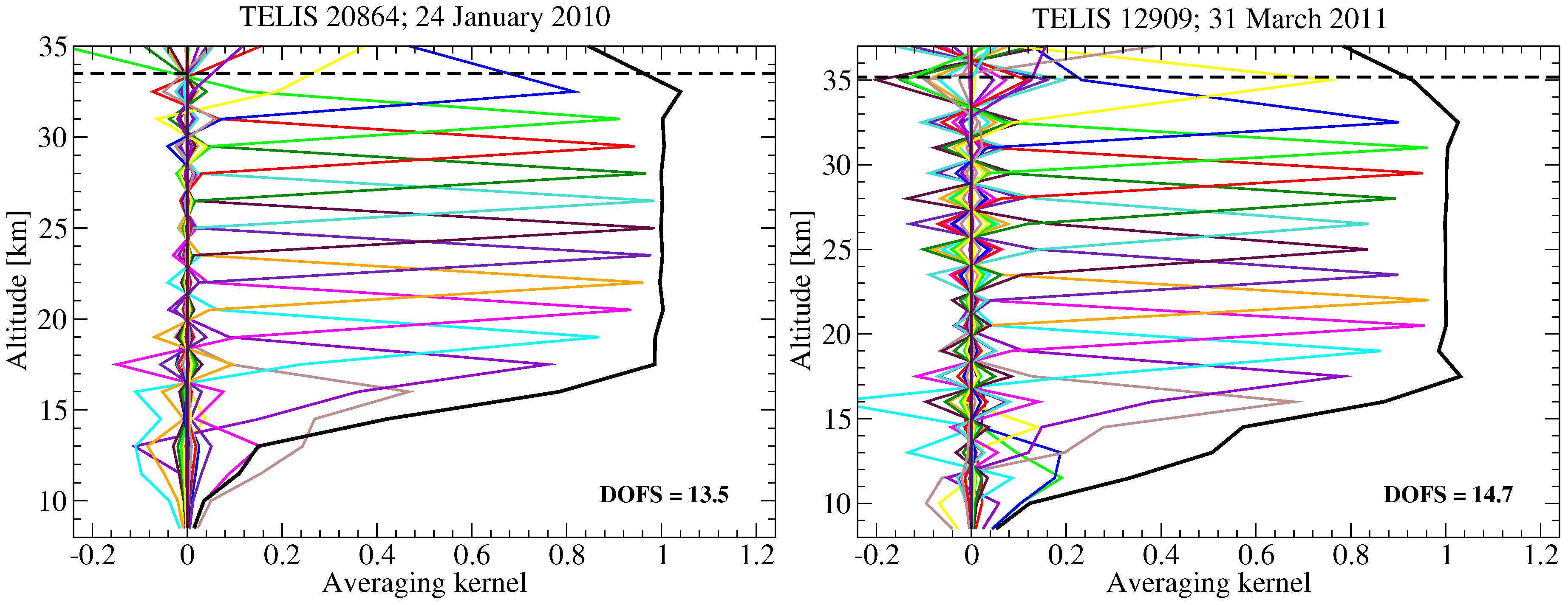
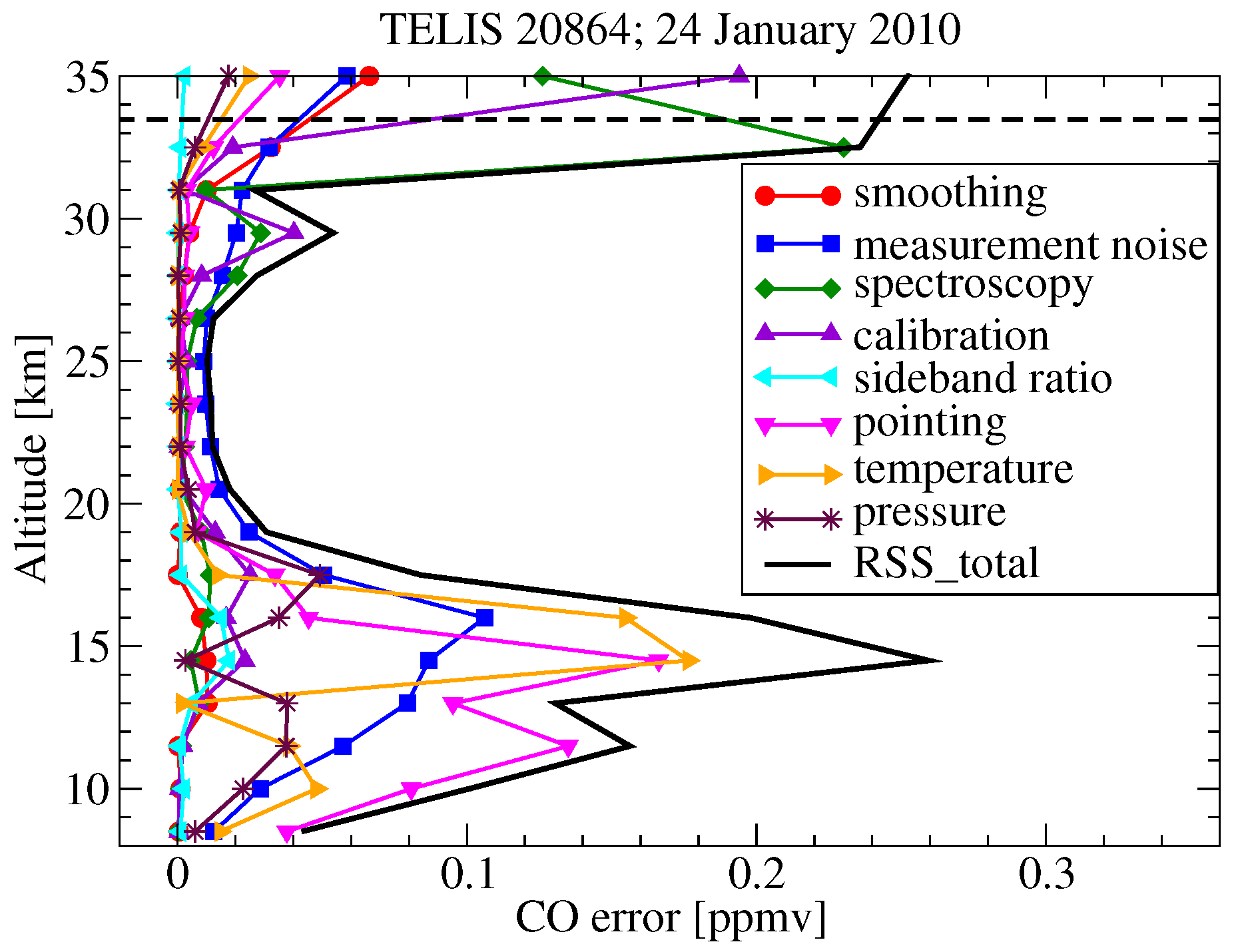
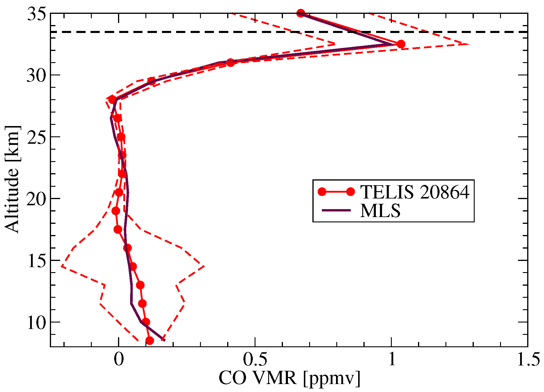
4.3. CO Retrieval
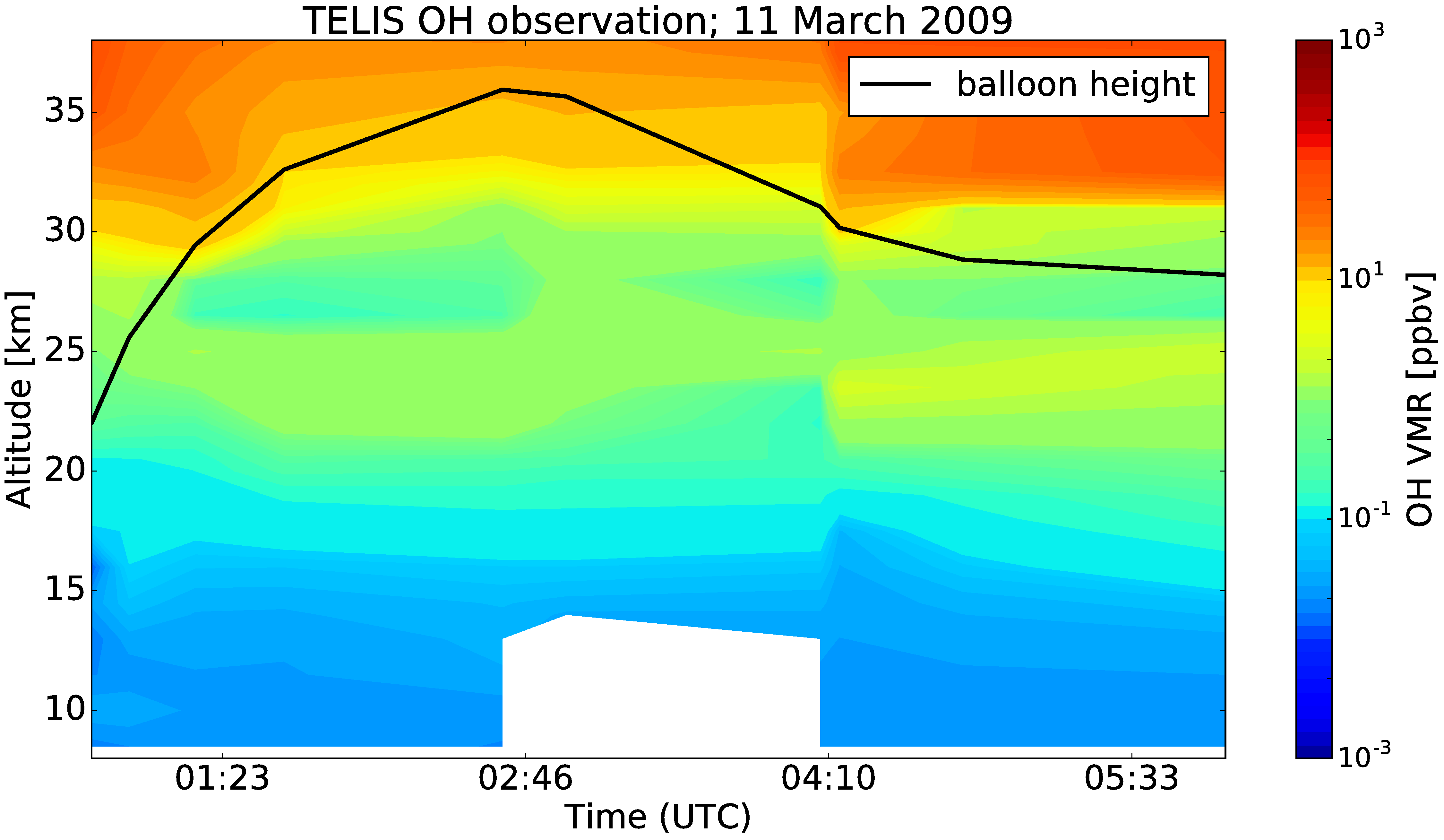
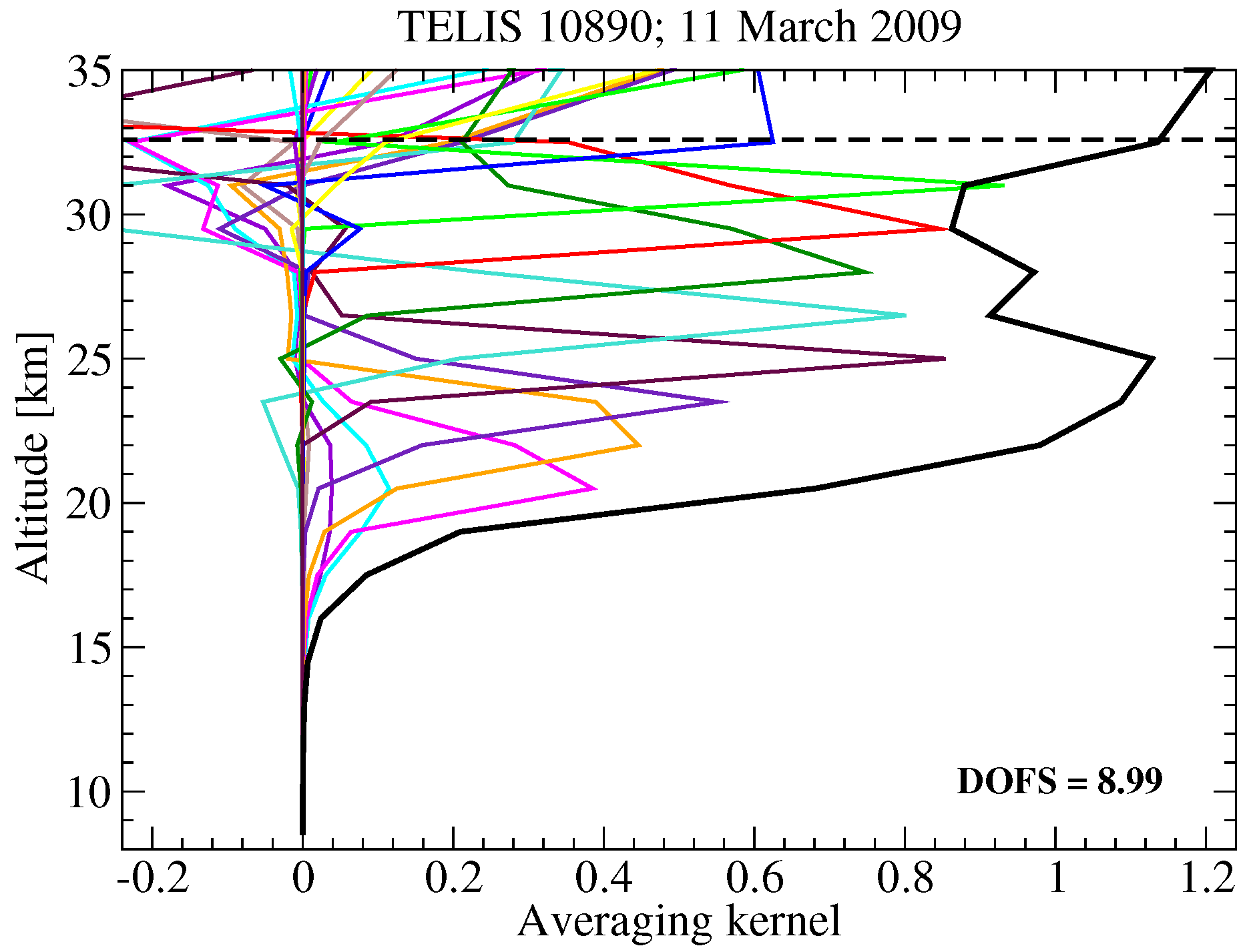
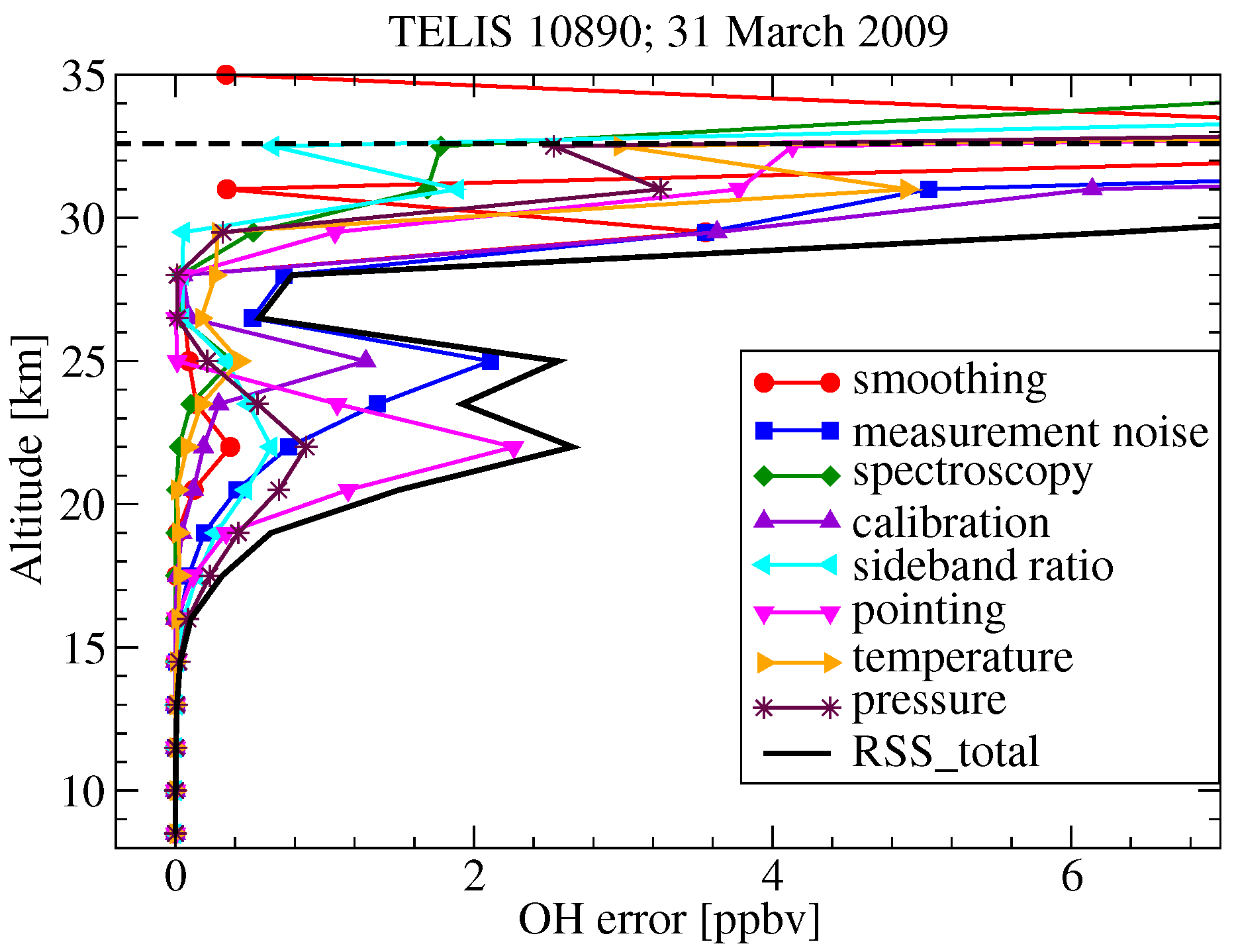
4.4. OH Retrieval
5. Conclusions
- concentration as a function of altitude;
- residual after convergence;
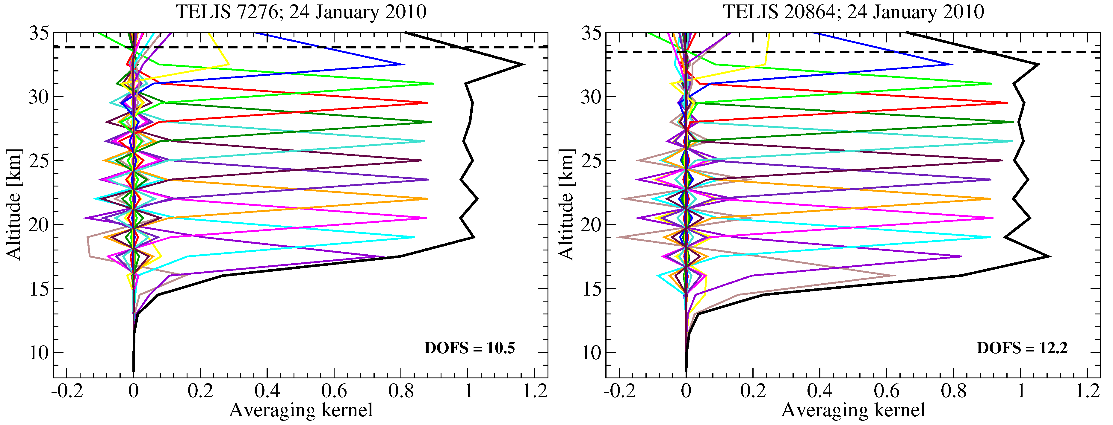
- retrieval diagnostics including an analysis of all considered error components and an averaging kernel matrix with DOFS.
Acknowledgments
Author Contributions
Conflicts of Interest
References
- Harries, J.; Carli, B.; Rizzi, R.; Serio, C.; Mlynczak, M.; Palchetti, L.; Maestri, T.; Brindley, H.; Masiello, G. The Far-infrared Earth. Rev. Geophys. 2008, 46. [Google Scholar] [CrossRef]
- Carli, B.; Mencaraglia, F.; Bonetti, A. Submillimeter high-resolution FT spectrometer for atmospheric studies. Appl. Opt. 1984, 23, 2594–2603. [Google Scholar] [CrossRef] [PubMed]
- Carli, B.; Park, J.H. Simultaneous measurement of minor stratospheric constituents with emission far-infrared spectroscopy. J. Geophys. Res. Atmos. 1988, 93, 3851–3865. [Google Scholar] [CrossRef]
- Carli, B.; Mencaraglia, F.; Carlotti, M.; Dinelli, B.M.; Nolt, I. Submillimeter measurements of stratospheric chlorine monoxide. J. Geophys. Res. Atmos. 1988, 93, 7063–7068. [Google Scholar] [CrossRef]
- Carli, B.; Carlotti, M.; Dinelli, B.; Mencaraglia, F.; Park, J. The mixing ratio of stratospheric hydroxyl radical from far infrared emission measurements. J. Geophys. Res. 1989, 94, 11049–11058. [Google Scholar] [CrossRef]
- Carlotti, M.; Barbis, A.; Carli, B. Stratospheric ozone vertical distribution from far-infrared balloon spectra and statistical analysis of the errors. J. Geophys. Res. Atmos. 1989, 94, 16365–16372. [Google Scholar] [CrossRef]
- Barath, F.T.; Chavez, M.C.; Cofield, R.E.; Flower, D.A.; Frerking, M.A.; Gram, M.B.; Harris, W.M.; Holden, J.R.; Jarnot, R.F.; Kloezeman, W.G.; et al. The Upper Atmosphere Research Satellite microwave limb sounder instrument. J. Geophys. Res. 1993, 98, 10751–10762. [Google Scholar] [CrossRef]
- Murtagh, D.; Frisk, U.; Merino, F.; Ridal, M.; Jonsson, A.; Stegman, J.; Witt, G.; Eriksson, P.; Jiménez, C.; Megie, G.; et al. An overview of the Odin atmospheric mission. Can. J. Phys. 2002, 80, 309–319. [Google Scholar] [CrossRef]
- Waters, J.; Froidevaux, L.; Harwood, R.; Jarnot, R.; Pickett, H.; Read, W.; Siegel, P.; Cofield, R.; Filipiak, M.; Flower, D.; et al. The Earth Observing System Microwave Limb Sounder (EOS MLS) on the Aura satellite. IEEE Trans. Geosci. Remote Sens. 2006, 44, 1075–1092. [Google Scholar] [CrossRef]
- Kikuchi, K.; Nishibori, T.; Ochiai, S.; Ozeki, H.; Irimajiri, Y.; Kasai, Y.; Koike, M.; Manabe, T.; Mizukoshi, K.; Murayama, Y.; et al. Overview and early results of the Superconducting Submillimeter-Wave Limb-Emission Sounder (SMILES). J. Geophys. Res. Atmos. 2010, 115. [Google Scholar] [CrossRef]
- Johnson, D.G.; Jucks, K.W.; Traub, W.A.; Chance, K.V. Smithsonian stratospheric far-infrared spectrometer and data reduction system. J. Geophys. Res. Atmos. 1995, 100, 3091–3106. [Google Scholar] [CrossRef]
- Chance, K.; Johnson, D.; Traub, W. Measurement of stratospheric HOCl: Concentration profiles, including diurnal variation. J. Geophys. Res. Atmos. 1989, 94, 11059–11069. [Google Scholar] [CrossRef]
- Traub, W.A.; Johnson, D.G.; Chance, K.V. Stratospheric Hydroperoxyl Measurements. Science 1990, 247, 446–449. [Google Scholar] [CrossRef] [PubMed]
- Chance, K.V.; Johnson, D.G.; Traub, W.A.; Jucks, K.W. Measurement of the stratospheric hydrogen peroxide concentration profile using far infrared thermal emission spectroscopy. Geophys. Res. Lett. 1991, 18, 1003–1006. [Google Scholar] [CrossRef]
- Jucks, K.; Johnson, D.; Chance, K.; Traub, W.; Margitan, J.; Osterman, G.; Salawitch, R.; Sasano, Y. Observations of OH, HO2, H2O, and O3 in the upper stratosphere: Implications for HOx photochemistry. Geophys. Res. Lett. 1998, 25, 3935–3938. [Google Scholar] [CrossRef]
- Friedl-Vallon, F.; Maucher, G.; Seefeldner, M.; Trieschmann, O.; Kleinert, A.; Lengel, A.; Keim, C.; Oelhaf, H.; Fischer, H. Design and characterization of the balloon-borne Michelson Interferometer for Passive Atmospheric Sounding (MIPAS-B2). Appl. Opt. 2004, 43, 3335–3355. [Google Scholar] [CrossRef] [PubMed]
- Fischer, H.; Birk, M.; Blom, C.; Carli, B.; Carlotti, M.; von Clarmann, T.; Delbouille, L.; Dudhia, A.; Ehhalt, D.; Endemann, M.; et al. MIPAS: An instrument for atmospheric and climate research. Atmos. Chem. Phys. 2008, 8, 2151–2188. [Google Scholar] [CrossRef]
- Höpfner, M.; von Clarmann, T.; Fischer, H.; Funke, B.; Glatthor, N.; Grabowski, U.; Kellmann, S.; Kiefer, M.; Linden, A.; Milz, M.; et al. Validation of MIPAS ClONO2 measurements. Atmos. Chem. Phys. 2007, 7, 257–281. [Google Scholar] [CrossRef]
- Wang, D.Y.; Höpfner, M.; Blom, C.E.; Ward, W.E.; Fischer, H.; Blumenstock, T.; Hase, F.; Keim, C.; Liu, G.Y.; Mikuteit, S.; et al. Validation of MIPAS HNO3 operational data. Atmos. Chem. Phys. 2007, 7, 4905–4934. [Google Scholar] [CrossRef]
- Wetzel, G.; Bracher, A.; Funke, B.; Goutail, F.; Hendrick, F.; Lambert, J.C.; Mikuteit, S.; Piccolo, C.; Pirre, M.; Bazureau, A.; et al. Validation of MIPAS-ENVISAT NO2 operational data. Atmos. Chem. Phys. 2007, 7, 3261–3284. [Google Scholar] [CrossRef]
- Zhang, G.; Wetzel, G.; Oelhaf, H.; Friedl-Vallon, F.; Kleinert, A.; Lengel, A.; Maucher, G.; Nordmeyer, H.; Grunow, K.; Fischer, H. Validation of temperature measurements from MIPAS-ENVISAT with balloon observations obtained by MIPAS-B. J. Atmos. Sol.-Terr. Phys. 2010, 72, 837–847. [Google Scholar]
- Zhang, G.; Wetzel, G.; Oelhaf, H.; Friedl-Vallon, F.; Kleinert, A.; Lengel, A.; Maucher, G.; Nordmeyer, H.; Grunow, K.; Fischer, H. Validation of atmospheric chemistry measurements from MIPAS, SCIAMACHY, GOMOS onboard ENVISAT by observations of balloon-borne MIPAS-B. Sci. China Earth Sci. 2010, 53, 1533–1541. [Google Scholar] [CrossRef]
- Wetzel, G.; Oelhaf, H.; Berthet, G.; Bracher, A.; Cornacchia, C.; Feist, D.G.; Fischer, H.; Fix, A.; Iarlori, M.; Kleinert, A.; et al. Validation of MIPAS-ENVISAT H2O operational data collected between July 2002 and March 2004. Atmos. Chem. Phys. 2013, 13, 5791–5811. [Google Scholar] [CrossRef] [Green Version]
- Wetzel, G.; Oelhaf, H.; Friedl-Vallon, F.; Kleinert, A.; Lengel, A.; Maucher, G.; Nordmeyer, H.; Ruhnke, R.; Nakajima, H.; Sasano, Y.; et al. Intercomparison and validation of ILAS-II version 1.4 target parameters with MIPAS-B measurements. J. Geophys. Res. Atmos. 2006, 111. [Google Scholar] [CrossRef]
- Sagawa, H.; Sato, T.O.; Baron, P.; Dupuy, E.; Livesey, N.; Urban, J.; von Clarmann, T.; de Lange, A.; Wetzel, G.; Connor, B.J.; et al. Comparison of SMILES ClO profiles with satellite, balloon-borne and ground-based measurements. Atmos. Meas. Tech. 2013, 6, 3325–3347. [Google Scholar] [CrossRef]
- Camy-Peyret, C.; Jeseck, P.; Hawat, T.; Durry, G.; Payan, S.; Berubé, G.; Rochette, L.; Huguenin, D. The LPMA balloon-borne FTIR spectrometer for remote sensing of atmospheric constituents. In Proceedings of the 12th ESA Symposium on European Rocket and Balloon Programmes and Related Research, Lillehammer, Norway, 29 May–1 June 1995; Kaldeich-Schürmann, B., Ed.; ESA Special Publication: Paris, France, 1995; SP-370, pp. 323–328. [Google Scholar]
- Irimajiri, Y.; Manabe, T.; Ochiai, S.; Masuko, H.; Yamagami, T.; Saito, Y.; Izutsu, N.; Kawasaki, T.; Namiki, M.; Murata, I. BSMILES—A balloon-borne superconducting submillimeter-wave limb-emission sounder for stratospheric measurements. IEEE Geosci. Remote Sens. Lett. 2006, 3, 88–92. [Google Scholar] [CrossRef]
- Waters, J.; Hardy, J.; Jarnot, R.; Pickett, H.; Zimmerman, P. A balloon-borne microwave limb sounder for stratospheric measurements. J. Quant. Spectrosc. Radiat. Transf. 1984, 32, 407–433. [Google Scholar] [CrossRef]
- Birk, M.; Wagner, G.; de Lange, G.; de Lange, A.; Ellison, B.N.; Harman, M.R.; Murk, A.; Oelhaf, H.; Maucher, G.; Sartorius, C. TELIS: TErahertz and subMMW LImb Sounder—Project Summary After First Sucessful Flight. In Proceedings of the 21st International Symposium on Space Terahertz Technology, Oxford and Didcot, UK, 23–25 March 2010; University of Oxford and STFC Rutherford Appleton Laboratory: Swindon, UK, 2010; pp. 195–200. [Google Scholar]
- Suttiwong, N.; Birk, M.; Wagner, G.; Krocka, M.; Wittkamp, M.; Haschberger, P.; Vogt, P.; Geiger, F. Development and characterization of the balloon borne instrument TELIS (TEhertz and Submm LImb Sounder): 1.8 THz receiver. In Proceedings of the 19th ESA Symposium on European Rocket and Balloon Programmes and Related Research, Bad Reichenhall, Germany, 7–11 June 2009. [Google Scholar]
- De Lange, G.; Birk, M.; Boersma, D.; Derckson, J.; Dmitriev, P.; Ermakov, A.; Filippenko, L.; Golstein, H.; Hoogeveen, R.; de Jong, L.; et al. Development and characterization of the superconducting integrated receiver channel of the TELIS atmospheric sounder. Supercond. Sci. Technol. 2010, 23. [Google Scholar] [CrossRef]
- Kasai, Y.; Sagawa, H.; Kreyling, D.; Dupuy, E.; Baron, P.; Mendrok, J.; Suzuki, K.; Sato, T.O.; Nishibori, T.; Mizobuchi, S.; et al. Validation of stratospheric and mesospheric ozone observed by SMILES from International Space Station. Atmos. Meas. Tech. 2013, 6, 2311–2338. [Google Scholar] [CrossRef]
- Eckert, E.; Laeng, A.; Lossow, S.; Kellmann, S.; Stiller, G.; von Clarmann, T.; Glatthor, N.; Höpfner, M.; Kiefer, M.; Oelhaf, H.; et al. MIPAS IMK/IAA CFC-11 (CCl3F) and CFC-12 (CCl2F2) measurements: Accuracy, precision and long-term stability. Atmos. Meas. Tech. 2016, 9, 3355–3389. [Google Scholar] [CrossRef]
- Koshelets, V.P.; Ermakov, A.B.; Filippenko, L.V.; Khudchenko, A.V.; Kiselev, O.S.; Sobolev, A.S.; Torgashin, M.Y.; Yagoubov, P.A.; Hoogeveen, R.W.M.; Wild, W. Superconducting Integrated Submillimeter Receiver for TELIS. IEEE Trans. Appl. Supercond. 2007, 17, 336–342. [Google Scholar] [CrossRef]
- Kiselev, O.; Birk, M.; Ermakov, A.; Filippenko, L.; Golstein, H.; Hoogeveen, R.; Kinev, N.; van Kuik, B.; de Lange, A.; de Lange, G.; et al. Balloon-borne superconducting integrated receiver for atmospheric research. IEEE Trans. Appl. Supercond. 2011, 21, 612–615. [Google Scholar] [CrossRef]
- Koshelets, V.P.; Dmitriev, P.N.; Faley, M.I.; Filippenko, L.V.; Kalashnikov, K.V.; Kinev, N.V.; Kiselev, O.S.; Artanov, A.A.; Rudakov, K.I.; de Lange, A.; et al. Superconducting Integrated Terahertz Spectrometers. IEEE Trans. Terahertz Sci. Technol. 2015, 5, 687–694. [Google Scholar] [CrossRef]
- Kiselev, O.S.; Ermakov, A.B.; Koshelets, V.P.; Filippenko, L.V. Application of superconducting integrated receiver in the TELIS instrument for the spectroscopic study of atmosphere. J. Commun. Technol. Electron. 2016, 61, 1314–1319. [Google Scholar] [CrossRef]
- De Lange, A.; Landgraf, J.; Hoogeveen, R. Stratospheric isotopic water profiles from a single submillimeter limb scan by TELIS. Atmos. Meas. Tech. 2009, 2, 423–435. [Google Scholar] [CrossRef]
- De Lange, A.; Birk, M.; de Lange, G.; Friedl-Vallon, F.; Kiselev, O.; Koshelets, V.; Maucher, G.; Oelhaf, H.; Selig, A.; Vogt, P.; et al. HCl and ClO in activated Arctic air; first retrieved vertical profiles from TELIS submillimetre limb spectra. Atmos. Meas. Tech. 2012, 5, 487–500. [Google Scholar] [CrossRef] [Green Version]
- Pickett, H. Microwave Limb Sounder THz module on Aura. IEEE Trans. Geosci. Remote Sens. 2006, 44, 1122–1130. [Google Scholar] [CrossRef]
- Englert, C.; Schimpf, B.; Birk, M.; Schreier, F.; Krocka, M.; Nitsche, R.; Titz, R.; Summers, M. The 2.5 THz heterodyne spectrometer THOMAS: Measurement of OH in the middle atmosphere and comparison with photochemical model results. J. Geophys. Res. Atmos. 2000, 105, 22211–22223. [Google Scholar] [CrossRef]
- Carlotti, M.; Ade, P.; Carli, B.; Chipperfield, M.; Hamilton, P.; Mencaraglia, F.; Nolt, I.; Ridolfi, M. Diurnal variability and night detection of stratospheric hydroxyl radical from far infrared emission measurements. J. Atmos. Sol.-Terr. Phys. 2001, 63, 1509–1518. [Google Scholar] [CrossRef]
- Pickett, H.M.; Peterson, D.B. Stratospheric OH measurements with a far-infrared limb observing spectrometer. J. Geophys. Res. Atmos. 1993, 98, 20507–20515. [Google Scholar] [CrossRef]
- Von Hobe, M.; Bekki, S.; Borrmann, S.; Cairo, F.; D’Amato, F.; Di Donfrancesco, G.; Dörnbrack, A.; Ebersoldt, A.; Ebert, M.; Emde, C.; et al. Reconciliation of essential process parameters for an enhanced predictability of Arctic stratospheric ozone loss and its climate interactions (RECONCILE): Activities and results. Atmos. Chem. Phys. 2013, 13, 9233–9268. [Google Scholar] [CrossRef] [Green Version]
- Zhang, J.; Tian, W.; Chipperfield, M.P.; Xie, F.; Huang, J. Persistent shift of the Arctic polar vortex towards the Eurasian continent in recent decades. Nat. Clim. Chang. 2016, 6, 1094–1099. [Google Scholar] [CrossRef]
- Arnone, E.; Castelli, E.; Papandrea, E.; Carlotti, M.; Dinelli, B.M. Extreme ozone depletion in the 2010–2011 Arctic winter stratosphere as observed by MIPAS/ENVISAT using a 2-D tomographic approach. Atmos. Chem. Phys. 2012, 12, 9149–9165. [Google Scholar] [CrossRef]
- Sagi, K.; Murtagh, D.; Urban, J.; Sagawa, H.; Kasai, Y. The use of SMILES data to study ozone loss in the Arctic winter 2009/2010 and comparison with Odin/SMR data using assimilation techniques. Atmos. Chem. Phys. 2014, 14, 12855–12869. [Google Scholar] [CrossRef]
- Woiwode, W.; Oelhaf, H.; Gulde, T.; Piesch, C.; Maucher, G.; Ebersoldt, A.; Keim, C.; Höpfner, M.; Khaykin, S.; Ravegnani, F.; et al. MIPAS-STR measurements in the Arctic UTLS in winter/spring 2010: Instrument characterization, retrieval and validation. Atmos. Meas. Tech. 2012, 5, 1205–1228. [Google Scholar] [CrossRef] [Green Version]
- Castelli, E.; Dinelli, B.M.; Del Bianco, S.; Gerber, D.; Moyna, B.P.; Siddans, R.; Kerridge, B.J.; Cortesi, U. Measurement of the Arctic UTLS composition in presence of clouds using millimetre-wave heterodyne spectroscopy. Atmos. Meas. Tech. 2013, 6, 2683–2701. [Google Scholar] [CrossRef] [Green Version]
- Jacobson, M.Z. Air Pollution and Global Warming: History, Science, and Solutions, 2nd ed.; Cambridge University Press: New York, NY, USA, 2012. [Google Scholar]
- Wetzel, G.; Oelhaf, H.; Kirner, O.; Friedl-Vallon, F.; Ruhnke, R.; Ebersoldt, A.; Kleinert, A.; Maucher, G.; Nordmeyer, H.; Orphal, J. Diurnal variations of reactive chlorine and nitrogen oxides observed by MIPAS-B inside the January 2010 Arctic vortex. Atmos. Chem. Phys. 2012, 12, 6581–6592. [Google Scholar] [CrossRef]
- Wetzel, G.; Oelhaf, H.; Birk, M.; de Lange, A.; Engel, A.; Friedl-Vallon, F.; Kirner, O.; Kleinert, A.; Maucher, G.; Nordmeyer, H.; et al. Partitioning and budget of inorganic and organic chlorine species observed by MIPAS-B and TELIS in the Arctic in March 2011. Atmos. Chem. Phys. 2015, 15, 8065–8076. [Google Scholar] [CrossRef] [Green Version]
- Allen, D.R.; Stanford, J.L.; López-Valverde, M.A.; Nakamura, N.; Lary, D.J.; Douglass, A.R.; Cerniglia, M.C.; Remedios, J.J.; Taylor, F.W. Observations of middle atmosphere CO from the UARS ISAMS during the early northern winter 1991/92. J. Atmos. Sci. 1999, 56, 563–583. [Google Scholar] [CrossRef]
- Wehr, T.; Bühler, S.; von Engeln, A.; Künzi, K.; Langen, J. Retrieval of stratospheric temperatures from spaceborne microwave limb sounding measurement. J. Geophys. Res. Atmos. 1998, 103, 25997–26006. [Google Scholar] [CrossRef]
- Von Engeln, A.; Langen, J.; Wehr, T.; Bühler, S.; Künzi, K. Retrieval of upper stratospheric and mesospheric temperature profiles from Millimeter-Wave Atmospheric Sounder data. J. Geophys. Res. Atmos. 1998, 103, 31735–31748. [Google Scholar] [CrossRef]
- Carlotti, M.; Ridolfi, M. Derivation of temperature and pressure from submillimetric limb observations. Appl. Opt. 1999, 38, 2398–2409. [Google Scholar] [CrossRef] [PubMed]
- Verdes, C.; Bühler, S.; von Engeln, A.; Kuhn, T.; Künzi, K.; Eriksson, P.; Sinnhuber, B.M. Pointing and temperature retrieval from millimeter–submillimeter limb soundings. J. Geophys. Res. Atmos. 2002, 107, ACH 10-1–ACH 10-24. [Google Scholar] [CrossRef]
- Von Engeln, A.; Bühler, S. Temperature profile determination from microwave oxygen emissions in limb sounding geometry. J. Geophys. Res. Atmos. 2002, 107, ACL 12-1–ACL 12-15. [Google Scholar] [CrossRef]
- Suttiwong, N. Development and Characteristics of the Balloon Borne Instrument TELIS (TEhertz and Submillimeter LImb Sounder): 1.8 THz Receiver. PhD Thesis, University of Bremen, Bremen, Germany, 25 October 2010. [Google Scholar]
- Xu, J.; Schreier, F.; Vogt, P.; Doicu, A.; Trautmann, T. A sensitivity study for far infrared balloon-borne limb emission sounding of stratospheric trace gases. Geosci. Instrum. Methods Data Syst. Discuss. 2013, 3, 251–303. [Google Scholar] [CrossRef] [Green Version]
- Xu, J. Inversion for Limb Infrared Atmospheric Sounding. PhD Thesis, Technische Universität München, Munich, Germany, 9 May 2015. [Google Scholar]
- Schreier, F.; Gimeno García, S.; Hedelt, P.; Hess, M.; Mendrok, J.; Vasquez, M.; Xu, J. GARLIC—A general purpose atmospheric radiative transfer line-by-line infrared-microwave code: Implementation and evaluation. J. Quant. Spectrosc. Radiat. Transf. 2014, 137, 29–50. [Google Scholar] [CrossRef]
- Doicu, A.; Schreier, F.; Hilgers, S.; Hess, M. Multi-parameter regularization method for atmospheric remote sensing. Comput. Phys. Commun. 2005, 165, 1–9. [Google Scholar] [CrossRef]
- Dennis, J., Jr.; Schnabel, R.B. Numerical Methods for Unconstrained Optimization and Nonlinear Equations; SIAM: Philadelphia, PA, USA, 1996. [Google Scholar]
- Griewank, A.; Walther, A. Evaluating Derivatives: Principles and Techniques of Algorithmic Differentiation, 2nd ed.; SIAM: Philadelphia, PA, USA, 2008. [Google Scholar]
- Neidinger, R.D. Introduction to Automatic Differentiation and MATLAB Object-Oriented Programming. SIAM Rev. 2010, 52, 545–563. [Google Scholar] [CrossRef]
- Schreier, F.; Gimeno García, S.; Vasquez, M.; Xu, J. Algorithmic vs. finite difference Jacobians for infrared atmospheric radiative transfer. J. Quant. Spectrosc. Radiat. Transf. 2015, 164, 147–160. [Google Scholar] [CrossRef]
- Hascoët, L.; Pascual, V. The Tapenade Automatic Differentiation tool: Principles, Model, and Specification. ACM Trans. Math. Softw. 2013, 39. [Google Scholar] [CrossRef]
- Bakushinskii, A. The problem of the convergence of the iteratively regularized Gauss–Newton method. Comput. Math. Math. Phys. 1992, 32, 1353–1359. [Google Scholar]
- Doicu, A.; Schreier, F.; Hess, M. Iteratively Regularized Gauss–Newton Method for Atmospheric Remote Sensing. Comput. Phys. Commun. 2002, 148, 214–226. [Google Scholar] [CrossRef]
- Morozov, V.A. On the solution of functional equations by the method of regularization. Sov. Math. Dokl. 1966, 7, 414–417. [Google Scholar]
- Engl, H.W. Discrepancy principles for Tikhonov regularization of ill-posed problems leading to optimal convergence rates. J. Optim. Theory Appl. 1987, 52, 209–215. [Google Scholar] [CrossRef]
- Xu, J.; Schreier, F.; Doicu, A.; Trautmann, T. Assessment of Tikhonov-type regularization methods for solving atmospheric inverse problems. J. Quant. Spectrosc. Radiat. Transf. 2016, 184, 274–286. [Google Scholar] [CrossRef]
- Wetzel, G.; Oelhaf, H.; Ruhnke, R.; Friedl-Vallon, F.; Kleinert, A.; Kouker, W.; Maucher, G.; Reddmann, T.; Seefeldner, M.; Stowasser, M.; et al. NOy partitioning and budget and its correlation with N2O in the Arctic vortex and in summer midlatitudes in 1997. J. Geophys. Res. Atmos. 2002, 107, ACH 3-1–ACH 3-10. [Google Scholar] [CrossRef]
- Anderson, G.; Clough, S.; Kneizys, F.; Chetwynd, J.; Shettle, E. AFGL Atmospheric Constituent Profiles (0–120 km); Technical Report TR-86-0110; AFGL: Palm Desert, CA, USA, 15 May 1986. [Google Scholar]
- Clough, S.; Kneizys, F.; Davies, R. Line Shape and the Water Vapor Continuum. Atmos. Res. 1989, 23, 229–241. [Google Scholar] [CrossRef]
- Rothman, L.; Gordon, I.; Babikov, Y.; Barbe, A.; Benner, D.C.; Bernath, P.; Birk, M.; Bizzocchi, L.; Boudon, V.; Brown, L.; et al. The HITRAN2012 molecular spectroscopic database. J. Quant. Spectrosc. Radiat. Transf. 2013, 130, 4–50. [Google Scholar] [CrossRef] [Green Version]
- Rinsland, C.P.; Zander, R.; Namkung, J.S.; Farmer, C.B.; Norton, R.H. Stratospheric infrared continuum absorptions observed by the ATMOS experiment. J. Geophys. Res. Atmos. 1989, 94, 16303–16322. [Google Scholar] [CrossRef]
- Ridolfi, M.; Carli, B.; Carlotti, M.; Clarmann, T.V.; Dinelli, B.M.; Dudhia, A.; Flaud, J.M.; Höpfner, M.; Morris, P.E.; Raspollini, P.; et al. Optimized forward model and retrieval scheme for MIPAS near-real-time data processing. Appl. Opt. 2000, 39, 1323–1340. [Google Scholar] [CrossRef] [PubMed]
- Stiller, G.; von Clarmann, T.; Funke, B.; Glatthor, N.; Hase, F.; Höpfner, M.; Linden, A. Sensitivity of trace gas abundances retrievals from infrared limb emission spectra to simplifying approximations in radiative transfer modelling. J. Quant. Spectrosc. Radiat. Transf. 2002, 72, 249–280. [Google Scholar] [CrossRef]
- Boone, C.D.; Nassar, R.; Walker, K.A.; Rochon, Y.; McLeod, S.D.; Rinsland, C.P.; Bernath, P.F. Retrievals for the atmospheric chemistry experiment Fourier-transform spectrometer. Appl. Opt. 2005, 44, 7218–7231. [Google Scholar] [CrossRef] [PubMed]
- Baron, P.; Urban, J.; Sagawa, H.; Möller, J.; Murtagh, D.P.; Mendrok, J.; Dupuy, E.; Sato, T.O.; Ochiai, S.; Suzuki, K.; et al. The Level 2 research product algorithms for the Superconducting Submillimeter-Wave Limb-Emission Sounder (SMILES). Atmos. Meas. Tech. 2011, 4, 2105–2124. [Google Scholar] [CrossRef] [Green Version]
- Urban, J.; Lautié, N.; Flochmoën, E.L.; Jiménez, C.; Eriksson, P.; Dupuy, E.; Amraoui, L.E.; Ekström, M.; Frisk, U.; Murtagh, D.; et al. Odin/SMR limb observations of stratospheric trace gases: Level 2 Processing of ClO, N2O, HNO3, and O3. J. Geophys. Res. Atmos. 2005, 110. [Google Scholar] [CrossRef]
- Pumphrey, H.C.; Bühler, S. Instrumental and spectral parameters: Their effort on and measurement by microwave limb sounding of the atmosphere. J. Quant. Spectrosc. Radiat. Transf. 2000, 64, 421–437. [Google Scholar]
- Buehler, S.A.; Verdes, C.L.; Tsujimaru, S.; Kleinböhl, A.; Bremer, H.; Sinnhuber, M.; Eriksson, P. Expected performance of the superconducting submillimeter-wave limb emission sounder compared with aircraft data. Radio Sci. 2005, 40, 1–13. [Google Scholar] [CrossRef]
- Vogt, P. Charakterisierung des ballongetragenen Heterodynspektrometers TELIS und erste Atmosphärische Messungen. Unpublished dissertation. 2013. [Google Scholar]
- Cortesi, U.; Lambert, J.C.; De Clercq, C.; Bianchini, G.; Blumenstock, T.; Bracher, A.; Castelli, E.; Catoire, V.; Chance, K.V.; De Mazière, M.; et al. Geophysical validation of MIPAS-ENVISAT operational ozone data. Atmos. Chem. Phys. 2007, 7, 4807–4867. [Google Scholar] [CrossRef]
- Steck, T.; von Clarmann, T.; Fischer, H.; Funke, B.; Glatthor, N.; Grabowski, U.; Höpfner, M.; Kellmann, S.; Kiefer, M.; Linden, A.; et al. Bias determination and precision validation of ozone profiles from MIPAS-Envisat retrieved with the IMK-IAA processor. Atmos. Chem. Phys. 2007, 7, 3639–3662. [Google Scholar] [CrossRef]
- Ochiai, S.; Kikuchi, K.; Nishibori, T.; Manabe, T.; Ozeki, H.; Mizobuchi, S.; Irimajiri, Y. Receiver performance of the Superconducting Submillimeter-Wave Limb-Emission Sounder (SMILES) on the International Space Station. IEEE Trans. Geosci. Remote Sens. 2013, 51, 3791–3802. [Google Scholar] [CrossRef]
- Sugita, T.; Kasai, Y.; Terao, Y.; Hayashida, S.; Manney, G.L.; Daffer, W.H.; Sagawa, H.; Suzuki, M.; Shiotani, M.; Walker, K.A.; et al. HCl and ClO profiles inside the Antarctic vortex as observed by SMILES in November 2009: Comparisons with MLS and ACE-FTS instruments. Atmos. Meas. Tech. 2013, 6, 3099–3113. [Google Scholar] [CrossRef]
- Livesey, N.; Van Snyder, W.; Read, W.; Wagner, P. Retrieval algorithms for the EOS Microwave Limb Sounder (MLS). IEEE Trans. Geosci. Remote Sens. 2006, 44, 1144–1155. [Google Scholar] [CrossRef]
- Jiang, Y.B.; Froidevaux, L.; Lambert, A.; Livesey, N.J.; Read, W.G.; Waters, J.W.; Bojkov, B.; Leblanc, T.; McDermid, I.S.; Godin-Beekmann, S.; et al. Validation of Aura Microwave Limb Sounder Ozone by ozonesonde and lidar measurements. J. Geophys. Res. Atmos. 2007, 112. [Google Scholar] [CrossRef] [Green Version]
- Pumphrey, H.C.; Filipiak, M.J.; Livesey, N.J.; Schwartz, M.J.; Boone, C.; Walker, K.A.; Bernath, P.; Ricaud, P.; Barret, B.; Clerbaux, C.; et al. Validation of middle-atmosphere carbon monoxide retrievals from the Microwave Limb Sounder on Aura. J. Geophys. Res. Atmos. 2007, 112. [Google Scholar] [CrossRef]
- Froidevaux, L.; Jiang, Y.B.; Lambert, A.; Livesey, N.J.; Read, W.G.; Waters, J.W.; Browell, E.V.; Hair, J.W.; Avery, M.A.; McGee, T.J.; et al. Validation of Aura Microwave Limb Sounder stratospheric ozone measurements. J. Geophys. Res. Atmos. 2008, 113. [Google Scholar] [CrossRef]
- Froidevaux, L.; Jiang, Y.B.; Lambert, A.; Livesey, N.J.; Read, W.G.; Waters, J.W.; Fuller, R.A.; Marcy, T.P.; Popp, P.J.; Gao, R.S.; et al. Validation of Aura Microwave Limb Sounder HCl measurements. J. Geophys. Res. Atmos. 2008, 113. [Google Scholar] [CrossRef] [Green Version]
- Livesey, N.J.; Filipiak, M.J.; Froidevaux, L.; Read, W.G.; Lambert, A.; Santee, M.L.; Jiang, J.H.; Pumphrey, H.C.; Waters, J.W.; Cofield, R.E.; et al. Validation of Aura Microwave Limb Sounder O3 and CO observations in the upper troposphere and lower stratosphere. J. Geophys. Res. Atmos. 2008, 113. [Google Scholar] [CrossRef]
- Jégou, F.; Urban, J.; de La Noë, J.; Ricaud, P.; Le Flochmoën, E.; Murtagh, D.P.; Eriksson, P.; Jones, A.; Petelina, S.; Llewellyn, E.J.; et al. Technical Note: Validation of Odin/SMR limb observations of ozone, comparisons with OSIRIS, POAM III, ground-based and balloon-borne instruments. Atmos. Chem. Phys. 2008, 8, 3385–3409. [Google Scholar] [CrossRef] [Green Version]
- Rodgers, C.D.; Connor, B.J. Intercomparison of remote sounding instruments. J. Geophys. Res. Atmos. 2003, 108. [Google Scholar] [CrossRef]
- Von Clarmann, T. Validation of remotely sensed profiles of atmospheric state variables: Strategies and terminology. Atmos. Chem. Phys. 2006, 6, 4311–4320. [Google Scholar] [CrossRef]
- Ridolfi, M.; Ceccherini, S.; Carli, B. Optimal interpolation method for intercomparison of atmospheric measurements. Opt. Lett. 2006, 31, 855–857. [Google Scholar] [CrossRef] [PubMed]
- Aires, F. Measure and exploitation of multisensor and multiwavelength synergy for remote sensing: 1. Theoretical considerations. J. Geophys. Res. Atmos. 2011, 116. [Google Scholar] [CrossRef] [Green Version]
- Landgraf, J.; Hasekamp, O.P. Retrieval of tropospheric ozone: The synergistic use of thermal infrared emission and ultraviolet reflectivity measurements from space. J. Geophys. Res. Atmos. 2007, 112. [Google Scholar] [CrossRef]
- Natraj, V.; Liu, X.; Kulawik, S.; Chance, K.; Chatfield, R.; Edwards, D.P.; Eldering, A.; Francis, G.; Kurosu, T.; Pickering, K.; et al. Multi-spectral sensitivity studies for the retrieval of tropospheric and lowermost tropospheric ozone from simulated clear-sky GEO-CAPE measurements. Atmos. Environ. 2011, 45, 7151–7165. [Google Scholar] [CrossRef]
- Cuesta, J.; Eremenko, M.; Liu, X.; Dufour, G.; Cai, Z.; Höpfner, M.; von Clarmann, T.; Sellitto, P.; Foret, G.; Gaubert, B.; et al. Satellite observation of lowermost tropospheric ozone by multispectral synergism of IASI thermal infrared and GOME-2 ultraviolet measurements over Europe. Atmos. Chem. Phys. 2013, 13, 9675–9693. [Google Scholar] [CrossRef] [Green Version]


| Retrieval Configuration | Description |
|---|---|
| Discretization | |
| Bottom-of-atmosphere | 8.5 or 14.5 km |
| Top-of-atmosphere | 65 km |
| 8.5–32.5 km (14.5–32.5 km) | 1.5 or 2 km |
| 32.5–40 km | 2.5 km |
| 40–65 km | 5 km |
| Temperature profile | MIPAS-B retrievals |
| Pressure profile | ECMWF |
| Remaining interfering species | AFGL subarctic winter model |
| Water vapor continuum | CKD model |
| Spectroscopic line parameters | HITRAN 2012 |
| Model Parameter Error | Perturbation |
|---|---|
| Spectroscopic parameters | |
| Line strength (S) | 1% (O3) |
| 2% (HCl) | |
| 1% (CO) | |
| 1% (OH) | |
| Air broadening (γair) | 5% |
| Temperature dependence (nair) | 10% |
| Radiometric calibration 1 | 5% |
| Sideband ratio | 0.05 |
| Pointing information | |
| Systematic bias | 3.4 arcmin |
| Uncertainty in the systematic bias | 1 arcmin |
| Atmospheric parameters | |
| Temperature | 1 K |
| Pressure | 1% |
| Position (cm−1) | Microwindow | Sideband | Segment(s) | Ei (cm−1) |
|---|---|---|---|---|
| 60.6502 | HDO | LSB | 4 | 1383.2810 |
| 60.9857 | HDO | USB | 1 | 828.9916 |
| 60.9895 | HDO | USB | 1–2 | 183.4307 |
| 61.0067 | HDO | USB | 2 | 1990.1950 |
| 61.0300 | HDO | USB | 4 | 1370.5580 |
| 61.1129 | CO | LSB | 1 | 286.8056 |
| 61.4391 | CO | USB | 3 | 1196.0930 |
| 61.4598 | CO | USB | 4 | 364.7143 |
© 2018 by the authors. Licensee MDPI, Basel, Switzerland. This article is an open access article distributed under the terms and conditions of the Creative Commons Attribution (CC BY) license (http://creativecommons.org/licenses/by/4.0/).
Share and Cite
Xu, J.; Schreier, F.; Wetzel, G.; De Lange, A.; Birk, M.; Trautmann, T.; Doicu, A.; Wagner, G. Performance Assessment of Balloon-Borne Trace Gas Sounding with the Terahertz Channel of TELIS. Remote Sens. 2018, 10, 315. https://doi.org/10.3390/rs10020315
Xu J, Schreier F, Wetzel G, De Lange A, Birk M, Trautmann T, Doicu A, Wagner G. Performance Assessment of Balloon-Borne Trace Gas Sounding with the Terahertz Channel of TELIS. Remote Sensing. 2018; 10(2):315. https://doi.org/10.3390/rs10020315
Chicago/Turabian StyleXu, Jian, Franz Schreier, Gerald Wetzel, Arno De Lange, Manfred Birk, Thomas Trautmann, Adrian Doicu, and Georg Wagner. 2018. "Performance Assessment of Balloon-Borne Trace Gas Sounding with the Terahertz Channel of TELIS" Remote Sensing 10, no. 2: 315. https://doi.org/10.3390/rs10020315