Article

Coherent Auto-Calibration of APE and NsRCM under Fast Back-Projection Image Formation for Airborne SAR Imaging in Highly-Squint Angle

1
Tianjin Key Laboratory for Advanced Signal Processing, Civil Aviation University of China, Tianjin 300300, China
2
School of Electronic Information and Engineering, Nanchang University, Nanchang 330031, China
3
School of Electrical and Electronic Engineering, Nanyang Technological University, 50 Nanyang Avenue, S2-B3a-06, 639798, Singapore
4
National Key Lab for Radar Signal Processing, Xidian University, Xi’an 710071, China
*
Author to whom correspondence should be addressed.
Current address: College of Electronic Information and Automation, D-301, Civil Aviation University of China (South), No. 2898, Tianjin Jinbei Road, Dongli District, Tianjin 300300, China.
Remote Sens. 2018, 10(2), 321; https://doi.org/10.3390/rs10020321
Submission received: 9 January 2018 / Revised: 9 January 2018 / Accepted: 18 February 2018 / Published: 21 February 2018

Abstract

:
Synthetic Aperture Radar (SAR) imaging with a non-zero (forward) squint angle is capable of providing a longer time for reaction than that of the broadside mode. However, due to the large squint angle, there will be severe coupling between range and azimuth samples in the echoed data, which is known as the problematic Range Cell Migration (RCM) in the SAR community. Especially when the SAR sensor mounted on an airborne platform encounters unexpected motion deviations/errors, the coupling becomes more complicated, and it is difficult to differentiate the systematic RCM for the SAR Image Formation Processing (IFP) and the non-systematic RCM error to be compensated. To this end, a novel and accurate SAR imaging algorithm is proposed in this paper to facilitate the processing of airborne SAR data collected at a high-squint angle. Firstly, the proposed algorithm is established under a Fast Time-Domain Back-Projection (FTDBP) framework for the SAR IFP. FTDBP paves the way to avoid the complicated processing for the systematic RCM as for the conventional SAR IFP in the Doppler processing manner. It is capable of generating a high-resolution SAR image efficiently under more general geometries and configurations. Secondly, regarding the non-systematic RCM errors, the proposed algorithm realizes the compensation by correcting both the Non-systematic Range Cell Migration (NsRCM), as well as Azimuthal Phase Error (APE) in a coherent manner. It is consequently capable of auto-calibrating the effects of the motion error completely without being dependent on the airborne navigation unit. Finally, both simulated and raw data collected by the airborne squinted SAR are applied to evaluate the proposed algorithm. Comparisons with conventional algorithms are carried out to reveal the superiority of the proposed algorithm.

Graphical Abstract

1. Introduction

Synthetic Aperture Radar (SAR) has become an important tool for ground mapping and remote sensing, because of its advantages of all weather, all day-and-night, long operating range and high spatial resolution [1,2,3,4,5]. SAR working in strip-map mode with the radar Line-of-Sight (LoS) in broadside can directly utilize iso-Doppler lines to achieve a large Doppler bandwidth, and accordingly, high spatial resolution SAR images can be obtained [1,2]. However, the broadside SAR will already pass the observing scene when the feature of the scene is figured out from the SAR image. To this end, by fixing the radar LoS at a forward non-zero squint angle, SAR is capable of providing sufficient time for reaction before the airborne radar arrives at the scene- or target-of-interest [1]. Consequently, the squint SAR is more flexible for practical applications, such as landing radar, guiding radar, warning radar, and so on [6].
SAR Image Formation Processing (IFP) for the broadside mode has been well established [1,2]. However, it is still a challenging problem for the squint SAR IFP. Due to the large squint angle, the complicated Range Cell Migration (RCM) is difficult to fully handle [7]. Conventionally, to correct the RCM, the SAR IFP algorithms are mainly borrowed from the broadside SAR IFP, which works in the range-Doppler domain under the azimuth-invariant assumption [8]. Generally, the conventional algorithms for the squint SAR IFP can be referred to as Doppler Processing Algorithms (DPAs) [6,9,10,11]. However, followed by the increasing demand to increase the squint angle, the problematic RCM becomes much more complicated to handle, especially in airborne SAR applications. As the airborne SAR encounters unavoidable motion errors, the fundamental azimuth-invariant assumption would not always be satisfied [12], and the conventional DPAs may not achieve a good performance [13,14,15]. Therefore, it becomes necessary to develop a more flexible and more general SAR IFP algorithm for high-squint SAR imagery.
In this paper, we follow the other trend of SAR IFP, Time-Domain Back-Projection (TDBP) [16,17,18,19,20]. TDBP directly accumulates the radar echoes into specific SAR image pixels, which therefore avoids the complicated correction of RCM for the decoupling. Compared with DPAs established under the assumption of azimuth-invariance, TDBP is more general and can be applied at an arbitrary squint angle, aircraft trajectory, multistatic antenna elements, and so on [12]. Even though research on TDBP started earlier than DPAs, the development of TDBP becomes significant again because it can be applied to various applications without too many limitations. More recently, several fast implementations for TDBP have come out, which has greatly accelerated its development [16,19,20]. Among various Fast TDBP (FTDBP) implementations, Fast Factorized Back-Projection (FFBP) is the most popular one [13,16]. By running back-projections in a recursive manner, FFBP successfully reduces the computational complexity of TDBP from O ( N 3 ) to O ( N 2 log 2 ( N ) ) , which is comparable to DPAs [16]. FFBP is therefore capable of accommodating the squint SAR data collection and simultaneously has high efficiency. Consequently, we are to devise a novel SAR IFP algorithm based on the FFBP framework to achieve accurate and efficient imaging performance for high-squint SAR data.
To process the airborne SAR data, the unavoidable airborne platform motion deviations/errors are some of the main concerns for achieving well-focused SAR images [1]. Due to the atmospheric turbulences and navigation errors, the airborne SAR frequently deviates from its predetermined flight track, and the motion errors will definitely affect the final SAR image quality. In general, the effects of motion errors on the SAR imagery are known as Non-systematic Range Cell Migration (NsRCM) and Azimuthal Phase Errors (APE) [21], where the former error induces range defocusing and affects the performance of the APE autofocusing, while the latter error leads to the azimuthal focusing degradation. To compensate the APE and NsRCM errors, the conventional way is to employ airborne Inertial Navigation Units and the Global Positioning System (INU/GPS) [12,13]. By directly measuring the motion deviations, it can be compensated before the SAR IFP. However, it would be insufficient in accuracy or even no measurements would be available for some radars with a limited budget for development [13,21]. Therefore, it becomes valuable and necessary to design an auto-calibration approach to estimate and compensate the motion errors in a data-driven manner.
The auto-calibration algorithms under DPAs have been well-developed [6,21,22]. In [21], for broadside SAR imaging, the authors designed a 2D motion error autofocusing algorithm that can adaptively calibrate the APE and NsRCM errors in a coherent manner. Although in [6,22], the squint SAR imagery is investigated under DPAs incorporating error auto-calibrations, the accuracy for high-squint and high-resolution data is limited. Because the DPAs have limited performance with respect squint SAR data, recently, FTDBP algorithms have been developed to incorporate data-driven auto-calibrations [12,13,19,23]. They are capable of facilitating the processing of the SAR data collected at a high-squint angle. In [13], a general spectrum under FFBP IFP algorithm is derived for broadside SAR imaging. Although a coherent relationship between the APE and NsRCM error is obtained, the along-track motion error is not taken into consideration when it is adopted in squint SAR imagery. In [23], FFBP was incorporated with auto-calibrations to process airborne squint SAR data, but without consideration of the NsRCM error. Consequently, it is necessary to develop an accurate and effective error auto-calibration algorithm under the FTDBP IFP framework for airborne squint SAR data.
In this paper, a novel squint SAR imaging algorithm is proposed under the FFBP IFP framework incorporated with a 2D error auto-calibration process that is capable of auto-calibrating both the APE and NsRCM errors in a coherent manner. Because both the motion errors in the along-track and cross-track are taken into account, the proposed algorithm can feasibly accommodate the airborne SAR data collected at a high-squint angle. FFBP, as one of implementations of FTDBP, is adopted for the SAR IFP. It therefore can avoid the complicated correction for the systematic RCM. This improves the applicability of the proposed algorithm for general applications without too many limitations. Analytical expressions for the APE and NsRCM errors are developed, and the relationship among APE, NsRCM and both the motion error in slant-range and along-track are explicitly revealed. Based on the analytical relationship, the error auto-calibration process can be completed by compensating the APE and NsRCM errors coherently, instead of separately. It therefore can achieve well-focused SAR images from the echoed data collected at a high-squint angle and even without the airborne navigation measurements or when only low accuracy measurements are available. A comprehensive review and discussion are given to show that the proposed algorithm is a general case of the previous models. Both simulated and raw SAR data collected at a large squint angle and from an airborne platform are used to evaluate the proposed algorithm.
The remainder of this paper is organized as follows. A general SAR geometry with a non-zero squint angle is established in Section 2, and the signal model is developed accordingly. In Section 3, FFBP as one of FTDBP implementations is employed for the SAR IFP. The motion error effects are analyzed and incorporated in Section 4. The detailed processing flowchart of the proposed algorithm is demonstrated in Section 5. Some useful discussions are carried out in Section 6. Simulations and raw data experiments are performed in Section 7. Finally, conclusions are drawn in Section 8.

2. Squint SAR Geometry and Signal Model

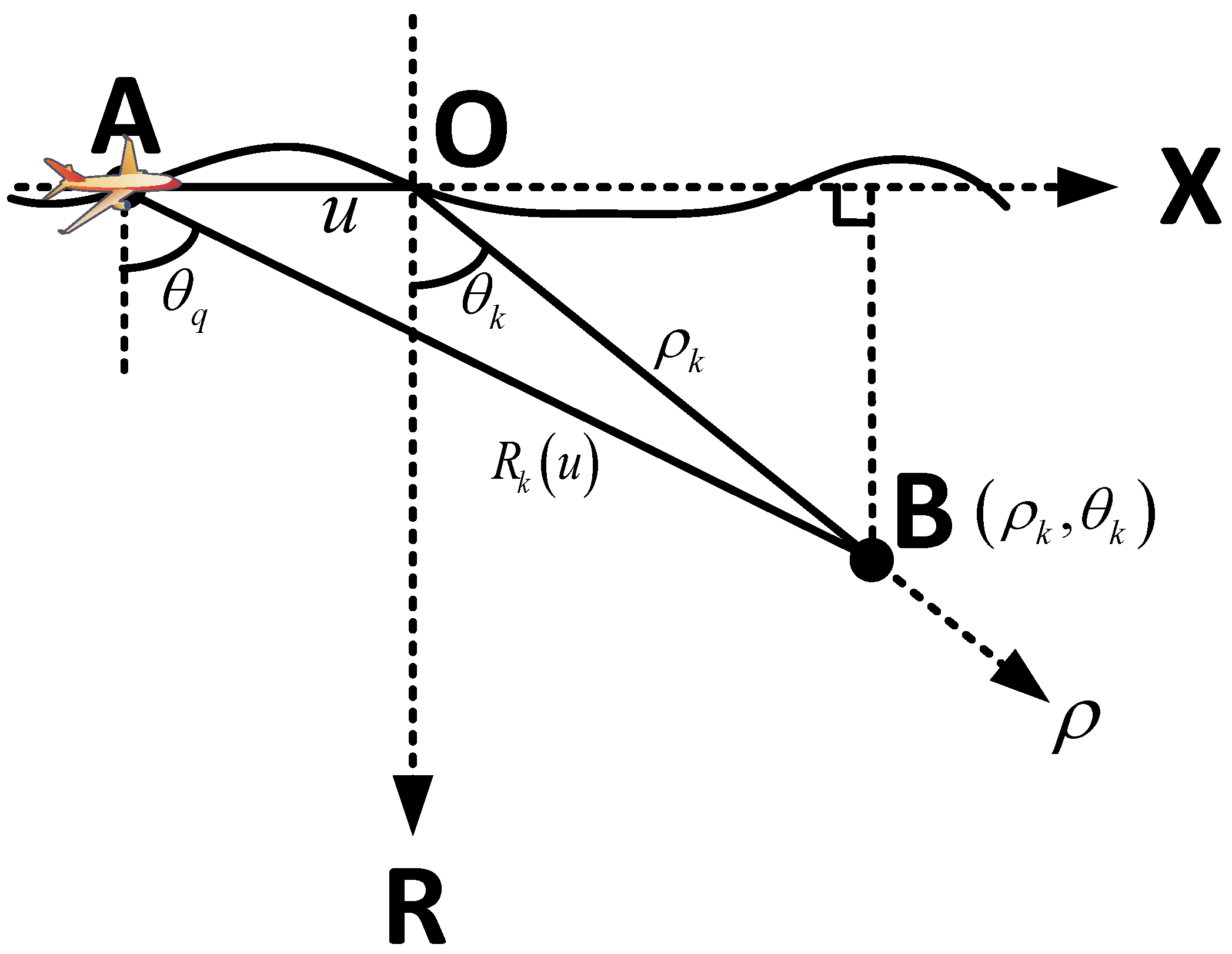
2.1. Squint SAR Geometry

The squint SAR geometry is demonstrated in Figure 1. As the two-dimensional (2D) SAR imaging problem is considered in this paper, the geometry is established in the slant-range plane [1]. The slant-range plane is denoted by X-O-R as shown in Figure 1, where the SAR sensor is mounted on an airborne platform flying along a predetermined flight track at a velocity of v. During the movement of the airborne radar, it transmits wideband pulses toward a ground scene to be imaged and collects the echoes simultaneously.
To image the ground scene-of-interest before the time when the airborne platform arrives, the radar LoS is directed with a forward squint angle θ q (Figure 1). Suppose an arbitrary ground scatter is represented in a polar grid with the coordinates ( ρ k , θ k ) . When the airborne SAR flies along the predetermined track, the range from the airborne radar (Position A in Figure 1) to the scatter (Position B) can be given according to the cosine formula as:
R k ( u ) = u 2 + ρ k 2 + 2 u ρ k cos ( π 2 + θ k )
where u represents the spatial variable of the synthetic aperture. This is the displacement of the airborne radar from the origin of the coordinates, and its variation can be determined according to the squint angle θ q and the radar beam width. By further manipulating Equation (1), we have:
R k ( u ) = u 2 + ρ k 2 2 u ρ k sin θ k .

2.2. Signal Model

It is well known that SAR generally transmits a series of wideband pulses at a constant Pulse Repetition Frequency (PRF) toward the ground scene-of-interest and collects the echoes simultaneously. With the round-trip of R k ( u ) in Equation (2), the echoed signal can be written as:
S ( k r , u ) = P ( k r ) k = 1 K exp [ j k r R k ( u ) ]
where in total, k ground scatters are considered, P ( k r ) denotes the spectrum of transmitted pulses and k r is the transmitting wavenumber. Giving f 0 as the centroid frequency and B as the bandwidth, we have k r = 4 π f r c and f r [ f 0 B 2 , f 0 + B 2 ] .
The echoed signal model in Equation (3) is established under a latent assumption that the airborne radar moves along a predetermined flight track. However, in practice, due to the atmospheric turbulence and navigation errors, the airborne platform inevitably encounters motion deviations from the predetermined ones [21], which will definitely influence the intended SAR imaging performance. The practical signal model can be therefore given as [21]:
S ˜ ( k r , u ) = S ( k r , u ) exp [ j k r Δ R ( u ) ]
where Δ R ( u ) generally represents the non-systematic range error from the airborne radar motion deviations. Only the space-independent range error is considered in Equation (4). Regrading that its is space-variant, interested readers can refer to [24] for solutions.
As can be noted from Equation (4), both in the systematic term S ( k r , u ) and the non-systematic term exp [ j k r Δ R ( u ) ] , the range wavenumber variable k r and the azimuth sample variable u are coupled with each other, which is known as the range migration. Generally, the designated SAR IFP is to remove the systematic coupling by correcting the range migration. In DPAs, the range migration is usually processed into Taylor series with respect to the azimuth sample variable. Then, the SAR IFP performs by generating matched-functions to correct the intended orders of the range migration [1]. Commonly, in the squint SAR imaging scenario, various orders of the range migration are desired to be corrected for a focused image. However, the separated order-by-order correction will definitely increase the complexity of the SAR IFP. Moreover, DPAs have limited performance for the high-squint SAR data due to the complexity.
Next, regrading the non-systematic range error Δ R ( u ) , it will lead to both the NsRCM and APE [21]. To quantificationally demonstrate the effect of the range error, the wavenumber variable k r is decomposed into k r = k 0 + Δ k r , and the error term k r Δ R ( u ) in Equation (4) can be decomposed as:
Δ ψ APE ( u ) = k 0 · Δ R ( u ) = 4 π f 0 c Δ R ( u ) = 4 π λ Δ R ( u )
and:
Δ ψ NsRCM ( Δ k r , u ) = Δ k r · Δ R ( u ) = 4 π Δ f r c Δ R ( u ) = 2 π Δ ρ r Δ R ( u )
where k 0 = 4 π f 0 c gives the wavenumber centroid, c is the speed of light, λ is the wavelength, Δ ρ r = c 2 Δ f r is the range resolution variation and Δ f r [ B 2 , B 2 ] . The degradation in Equation (5) is explained as the APE [21], where the range error Δ R ( u ) is evaluated by the wavelength λ . Therefore, the accuracy of the adjustment of APE can be interpreted by the radar wavelength. The APE commonly results in azimuthal focusing degradation, such as a widened main-lobe and increase sidelobes. Next, in Equation (6), the degradation is related to the azimuthal variable u and the range variable Δ ρ r ; therefore, Δ ψ NsRCM ( Δ k r , u ) or Δ ψ NsRCM ( Δ f r , u ) is known as the NsRCM error, which is a 2D error function that will lead to both range defocusing, as well as the azimuth autofocusing degradation. By further noticing Equation (6), the range error Δ R ( u ) is denoted with respect to the range resolution variation Δ ρ r , which can therefore be known as that the accuracy of the alignment of NsRCM is related to the range resolution. Following the development of modern SAR, both high-resolution and high-accuracy SAR imaging performances are desired. Consequently, both APE and NsRCM errors are to be compensated for a well-focused SAR image.
To this end, conventionally, the airborne INU/GPS is employed to measure the actual flight track. However, in some cases, only the instruments with coarse accuracy are available or even none of the instruments are available. Therefore, we have to rely on the data-driven approach [25]. In general, the data-driven motion error compensation method should be properly designed to incorporate the SAR IFP. For DPAs, it requires that the echoed spectrum obeys the azimuthal-invariance characteristic; unfortunately, the airborne SAR flight deviation will definitely violate this requirement, and the performance of both the IFP and the error auto-calibration will be degraded. Besides, due to the large squint angle, the projected along-track motion error (except the motion error projected onto the LoS) also should be taken into account.
In summery, to further improve the performance of the accommodation of high-squint SAR data and seamlessly incorporate the data-driven auto-calibration, in this paper, we choose the other trend of SAR IFP, that is the Time-Domain Back-Projection (TDBP) or, specifically, the Fast Factorized Back-Projection (FFBP). Details about FFBP will be introduced in the next section.

3. Fast Factorized Back-Projection

TDBP is a general SAR IFP approach that came out even earlier than DPAs. Different from DPAs, it directly processes the SAR echoes in the time-domain by BP processing, where each echoed pulse is accumulated into specific SAR image pixels [16], rather than transforming the pulses into the Doppler domain. There is no need for TDBP to satisfy the azimuth-invariant assumption, and there is no need to process the complicated range migration. Therefore, TDBP is more general than DPAs, and it can be applied in various SAR applications without limitations on squint angle, flight track and multistatic antennas [13]. Mathematically, TDBP achieves SAR images by directly integrating the echoes as:
I ρ , θ = S ˜ k r , u exp j k r u 2 + ρ 2 2 u ρ sin θ d k r d u ,
where ρ and θ give the axes in radial and angle dimensions, respectively. Using a simple transformation of coordinates, the polar grid image I ρ , θ in Equation (7) can be transformed in to the common Cartesian grid as I x , r on the slant-range plane.
To utilize the superiority of TDBP in high-squint SAR imaging, a fast implementation of TDBP, FFBP [16], is employed in this paper for the framework of SAR IFP. FFBP is the most classic TDBP that is capable of achieving a comparative accuracy of BP and simultaneously maintaining a high computational efficiency. The conventional FFBP usually performs in the polar coordinates in which the range of the frequency variation can be compacted into a narrower bandwidth so that the Nyquist sampling rate, as well as the number of BP operations can be dramatically reduced [12,17]. Different from the BP algorithm, FFBP performs in a recursive manner. An illustration of the recursion is shown in Figure 2.
In the FFBP recursion, the collected SAR data in the full synthetic aperture will be divided into several sub-apertures. In each sub-aperture, a coarse image will be generated by the BP operation. Next, as shown in Figure 2, the adjacent two sub-apertures are merged into a SAR image with higher resolution than that in the last recursion [16]. During the merging process, each pixel in the ( K + 1 ) -th sub-image is calculated from the corresponding pixels in K-th sub-images, as shown by the dashed arrows in Figure 2, and 2D interpolation will be utilized for calculating the pixels in the process. Following the recursion process, the length of sub-aperture increases, the number of sub-apertures decreases and the angular resolution of the SAR image becomes higher. As can be noted from Figure 2, from the K-th to the ( K + 1 ) -th recursion, the merged SAR image in the polar grid has higher angular resolution. The recursion runs until the final resolution achieves that corresponding to the full aperture. The choice of the number of recursions K is determined according to the length of the sub-aperture and the full-aperture. For simplicity, from the N divided sub-apertures, we have the number of the merging recursions as K log 2 ( N ) .
From the above analysis, thanks to the SAR IFP being carried out in the time-domain, the complicated process for the correction of range migration as for conventional DPAs can be avoided. Furthermore, in this paper, different from the commonly-used FFBP formation based on the polar grid, we introduce a novel FFBP formation that is derived in the quasi-polar grid [13]. The quasi-polar based FFBP formation makes it easy to estimate the motion error in the post-IFP data domain in a data-driven manner [13]. Specifically, when the FFBP proceeds in the quasi-polar grid ( ρ , x ) , the formed SAR image can be shown as:
I ρ , x = S ˜ k r , u exp j k r u 2 + ρ 2 2 u x d k r d u ,
where ρ and x = ρ sin θ represent the axes in the radial and along-track (or azimuth) directions, respectively. Then, two wavenumber variables, k ρ and k x , are introduced, which give the radial and along-track wavenumber variables, respectively. Under the commonly-used narrow-beam and far-field assumptions, Equation (8) can be approximated as: [13]
I ρ , x k = 1 K P ( k ρ ) exp ( j k ρ ρ k j k x x k ) exp ( k ρ Δ ρ ( u ) + k x Δ x ( u ) ) exp ( j k ρ ρ + j k x x ) d k ρ d k x
where x k = ρ k sin θ k and Δ ρ ( u ) and Δ x ( u ) are the components of the range error Δ R ( u ) in the radial and along-track directions, respectively. For detailed derivation of (9), refer to [13].

4. Motion Error Auto-Calibration

To facilitate the following analysis, the spatial variable u is substituted by [13]:
u = ρ 0 k x k ρ .
where ρ 0 gives the reference slant range from the radar to the observing scene center. Generally, the motion error compensation is carried out with respect to a reference point that is usually selected as the observing scene center. Next, both the motion error effects, APE and NsRCM errors are to be analyzed analytically, and a coherent error auto-calibration algorithm will be proposed under an analytical relationship between the errors.

4.1. Motion Error Effects

As seen in Equation (9), FFBP simply avoids the decoupling for the range migration, and both the radial and azimuthal coordinates of the k-th scatter, ρ k and x k are decoupled from the radial and along-track wavenumber k ρ and k x , respectively. Next, we are to solve the motion error problem. The signal model in Equation (9) can be shown in the 2D wavenumber domain as:
S ˜ ( k ρ , k x ) k = 1 K P ( k ρ ) exp ( j k ρ ρ k j k x x k ) exp [ k ρ Δ ρ ( u ) + k x Δ x ( u ) ] .
Equation (11) gives the analytical form of the error-contaminated echoes after FFBP SAR IFP. It can be noted from Equation (11) that each scatterer with the radial and azimuthal coordinates, ρ k and x k , can be easily imaged in the quasi-polar grid ( ρ , x ) by employing the Fourier Transformation (FT) with respect to k ρ and k x . However, due to the error, the image quality will be degraded. To evaluate the motion error effect, Equation (10) is substituted into Equation (11), and we have:
S ˜ ( k ρ , k x ) k = 1 K P ( k ρ ) exp ( j k ρ ρ k j k x x k ) exp [ k ρ Δ ρ ( ρ 0 k x k ρ ) + k x Δ x ( ρ 0 k x k ρ ) ] .
In Equation (12), the first exponential term gives the ground scatterer at the quasi-polar coordinates ( ρ k , x k ) , while the last exponential term shows the effect from the motion error. The first term in the error exponent represents the motion error effect from the airborne radar motion deviation in the radial direction, while the second term gives that in the along-track direction. By approximating the radial motion error effect in Taylor series expansion, there is:
k ρ Δ ρ ( ρ 0 k x k ρ ) k 0 Δ ρ ( ρ 0 k x k 0 ) + [ Δ ρ ( ρ 0 k x k 0 ) + ρ 0 k x k 0 Δ ρ ( ρ 0 k x k 0 ) ] ( k ρ k 0 )
where Δ ρ ( · ) gives the derivative of Δ ρ ( · ) . It can be noted from Equation (13) that the first term is proportional to the radial error Δ ρ ( · ) with a constant coefficient, i.e., the wavenumber centroid k 0 . It is therefore referred to as APE varying with the azimuth wavenumber variable k x . The other two terms in Equation (13) are represented with a common term ( k ρ k 0 ) , and both terms can be interpreted as the NsRCM error, which may result in a range cell migration error when [ Δ ρ ( ρ 0 k x k 0 ) + ρ 0 k x k 0 Δ ρ ( ρ 0 k x k 0 ) ] exceeds one range cell.
Next, in Equation (12), the second term in the exponential error function corresponding to the along-track motion error will also introduce degradations, and it can be analyzed similarly as:
k x Δ x ( ρ 0 k x k ρ ) k x Δ x ( ρ 0 k x k 0 ) + ρ 0 k x 2 k 0 2 Δ x ( ρ 0 k x k 0 ) ( k ρ k 0 )
where Δ x ( · ) represents the derivative of Δ x ( · ) . Similar to the above analysis, the first term in Equation (14) is known as the APE error function, and the residuals can be referred to as the NsRCM error.
Different from the conventions, both the APE and NsRCM errors are considered in the proposed error auto-calibration. Moreover, the errors are estimated and compensated coherently, instead of separately. As can be noted from Equations (13) and (14), both the radial and along-track motion errors will result in the APE and NsRCM errors. It is actually one of the contributions in this paper where both the radial and along-track motion errors are considered in the proposed error auto-calibration. In total, the NsRCM error can be therefore given as:
Δ R NsRCM ( k x ) = Δ ρ ( ρ 0 k x k 0 ) + ρ 0 k x k 0 Δ ρ ( ρ 0 k x k 0 ) + ρ 0 k x 2 k 0 2 Δ x ( ρ 0 k x k 0 ) .
Applying an Inverse FT (IFT) on the radial wavenumber in Equation (12), the expression for the range-compressed signal can be written as:
s ˜ ( ρ , k x ) = 1 2 π S ˜ ( k ρ , k x ) exp ( j k ρ ρ ) d k ρ .
Assuming p ( ρ ) represents the range profile that is determined by the specific form of P ( k ρ ) , the range-compressed signal can be re-written as:
s ˜ ( ρ , k x ) = k = 1 K p [ ρ ρ k Δ R NsRCM ( k x ) ] exp ( j k x x k ) exp [ j Δ ϕ APE ( k x ) ]
where:
Δ ϕ APE ( k x ) = k 0 Δ ρ ( ρ 0 k x k 0 ) + k x Δ x ( ρ 0 k x k 0 )
gives the total APE function from both the errors in radial and along-track directions. As can be noted in Equation (17), the range-compressed profile p [ · ] will shift due to the NsRCM error Δ R NsRCM in Equation (15). This will result in the range response of scatters in one range cell dispersing into adjacent range cells. It will also affect the performance of the auto-calibration process for the APE adjustment. Next, another IFT is performed on Equation (17) with respect to the azimuth wavenumber k x , and the SAR image can be therefore obtained as:
I ( ρ , x ) = 1 2 π s ˜ ( ρ , k x ) exp ( j k x x ) d k x .
where s ˜ ( ρ , k x ) can refer to Equation (17). Due to the unknown APE error Δ ϕ APE ( k x ) in s ˜ ( ρ , k x ) , the IFT operation in Equation (19) cannot fulfill the azimuthal focusing.

4.2. Coherent Relationship between APE and RCM

In this paper, we are to compensate the APE and NsRCM errors simultaneously in a coherent manner based on the FFBP formation. This is different from the conventions they implement in both the estimation and compensation separately. The conventions may take advantage of an arbitrary error function, but at the cost of efficiency. Generally, for SAR data, they inherently have coherence, which means the amplitude and phase modulation of the data have a coherent relationship. In other words, the range profile migration and the phase modulation should have a fixed relationship [12,13]. Thanks to the coherence, we can exploit the analytical form of the relationship between the APE and NsRCM error functions. When the relationship can be revealed after the SAR IFP, we can implement the 2D auto-calibration coherently. By further exploiting the NsRCM and APE error functions in Equations (15) and (18), an explicit relationship can be revealed as:
Δ R NsRCM ( k x ) = 1 k 0 [ Δ ϕ APE ( k x ) k x · Δ ϕ APE ( k x ) ] .
It can be clearly seen from Equation (20) that the NsRCM range error can be denoted by the APE error function with both its own terms and its derivative. This naturally paves the way to achieve both the error functions from one single error estimation. We will discuss details about the APE and NsRCM compensations in the next sub-section.
Compared to the APE and NsRCM errors before the SAR IFP as shown in Equations (5) and (6), it can be noted that the relationship has been changed after the FFBP SAR IFP. Before the SAR IFP, the APE and NsRCM errors are straightforwardly proportional within the same range error Δ R ( u ) ; while after FFBP in Equations (15) and (18), both error functions change into the combination of the range error and its derivative. The deterministic relationship between the APE and NsRCM errors reveals that the FFBP formation introduces an additional term of the error derivative. Without the relationship, both the APE and NsRCM errors should be estimated and compensated separately. With the analytical relationship, we can achieve one of the error functions under the estimation of the other, where a simple numerical calculation can replace the estimation of either APE or NsRCM error. Moreover, both errors in the radial and along-track directions are considered in the above development, which will facilitate the processing of the SAR data collected at a large squint angle.

4.3. Coherent Motion Error Compensation

Finally, both the APE and NsRCM errors are to be removed from the SAR echoes, so that the final SAR image can be well focused. As mentioned in the above sub-section, under the deterministic relationship in Equation (20), they can be estimated and compensated in a coherent manner.
Generally, both the APE and NsRCM errors can be estimated from the echoed data in the data-driven manner. Firstly, the APE error function can be estimated in the complex range-compressed data domain. By extracting the phase component of the echoed data from either a single range cell or multiple weighted cells, the phase error function can be estimated in various ways. In terms of the estimated phase type, there are three categories for the APE estimation, the phase rate estimation, the phase difference estimation and the direct phase estimation. Map-Drift (MD) [25], Phase Gradient Autofocusing (PGA) [21] and Minimum Entropy Autofocusing (MEA) [26] are the typical methods, respectively. Considering both the accuracy and efficiency of the APE error estimation, PGA is the best candidate, which has been widely used in the SAR community. Secondly, for the NsRCM error, it can be estimated by either calculating the correlation of the range profiles or evaluating an objective function of the entropy of the range profiles. The former requires the echoes to have a high signal-to-noise ratio (SNR), while the latter have a large computational burden.
Recall the relationship developed in Equation (20); it paves a way toward achieving the APE and NsRCM errors by firstly estimating one of them and then simply calculating the other according to the relationship. As it is well known that the accuracy of the error estimation from APE is higher than that from the NsRCM error, we propose the motion error compensation in a coherent manner under the relationship developed in Equation (20), where the APE estimation is performed first and then directly calculating the NsRCM error based on the analytical relationship. The coherent error auto-calibration can be therefore established. Furthermore, to estimate the APE error function, PGAs are to be adopted. To accommodate practical imaging scenarios, PGA is further improved as the Weighted PGA (WPGA) [21], which fully utilizes the phase redundancy across the range cells. Because WPGA is capable of achieving a high accuracy for an arbitrary error form and simultaneously maintaining a high efficiency, it is employed in the proposed algorithm. Followed by the APE estimation by WPGA, the NsRCM error function can be calculated according to Equation (20); both errors can be simultaneously compensated, and the proposed error auto-calibration method can accommodate arbitrary error forms of both APE and NsRCM errors.

5. Processing Procedure

In this section, the processing procedure of the proposed algorithm is presented, and the flowchart is demonstrated in Figure 3. Specifically, the processing procedure is carried out in three stages.
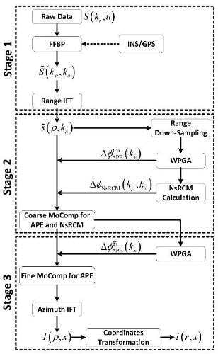
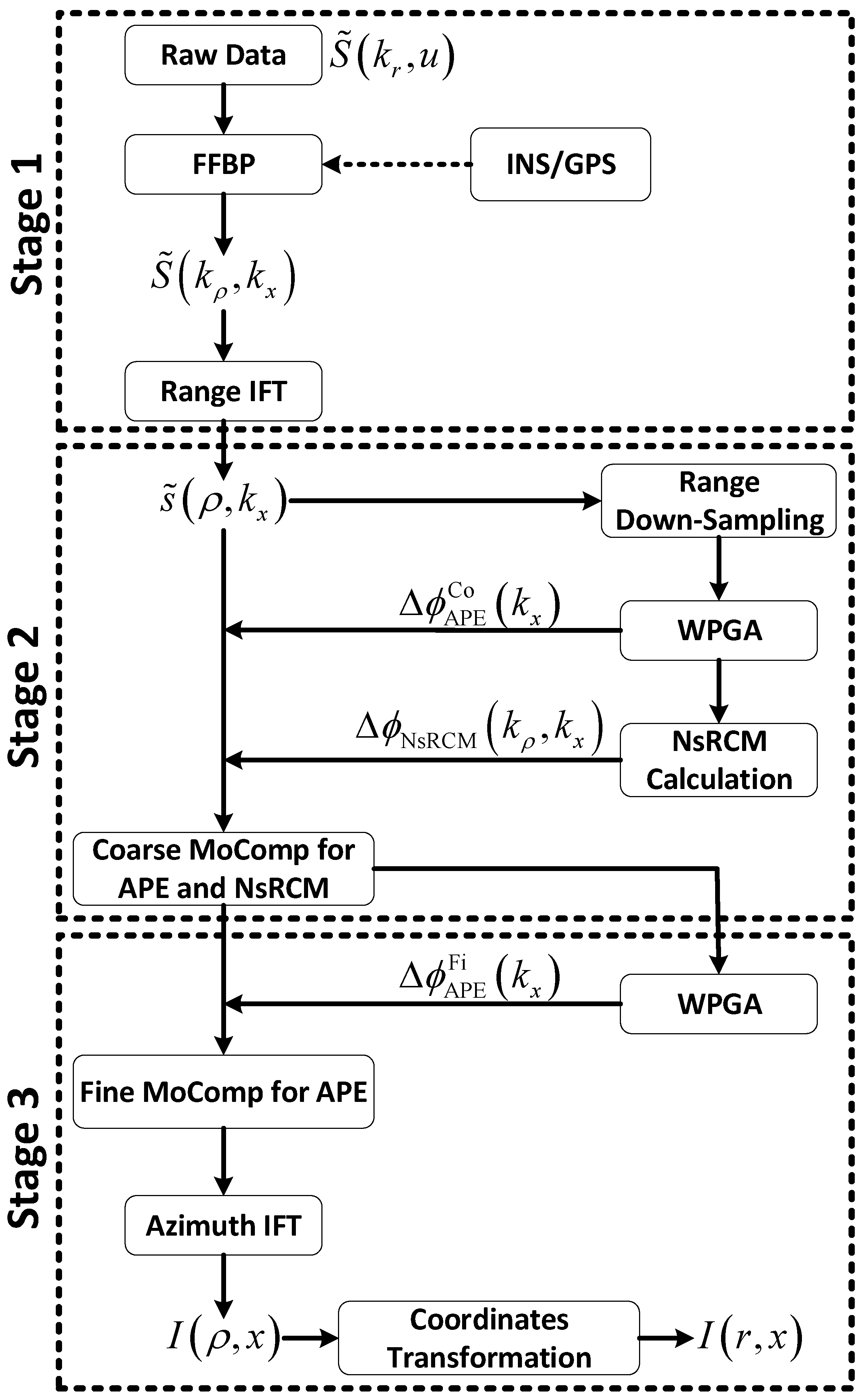
  • Stage 1: FFBP SAR IFP. At the first stage, the raw data collected at a large squint angle will be pre-processed. Either matched-filtering or de-chirping can be applied for the range de-ramp. Then, the data S ˜ ( k r , u ) as described in Equation (4) are processed by FFBP for the SAR IFP. FFBP as one of the classic FTDBP algorithms is capable of generating high-resolution SAR images without limitation on the squint angle. To accommodate the airborne application, if the airborne INU and GPS are available, they can be useful to preliminarily compensate the airborne SAR motion deviations/errors [25]. When no navigational data are available or only low accuracy data are available, the proposed algorithm still has the capability to compensate the error in a data-driven manner. To facilitate the FFBP SAR IFP with the data-driven error auto-calibration, the novel FFBP implementation in a quasi-polar grid is employed [13], and the data are transformed into the 2D wavenumber domain as S ˜ ( k ρ , k x ) in Equation (12). For the following motion error compensation, the data are further transformed into the range-compressed domain by a range IFT.
  • Stage 2: Coarse auto-calibration. At the second stage, the error auto-calibration process is carried out in the range-compressed data domain as s ˜ ( ρ , k x ) in Equation (17). To reduce the influence of the NsRCM on the APE estimation, range down-sampling will be performed [21]. Then, WPGA is employed to achieve the APE estimation Δ ϕ APE Co ( k x ) . According to the relationship developed in Equation (20), the NsRCM error function can be simply calculated as Δ ϕ NsRCM ( k ρ , k x ) . Accordingly, a coarse Motion error Compensation (MoComp) can be implemented with a coarse compensation for the APE and simultaneously a complete compensation for the NsRCM error. Though only a relatively coarse accuracy of the APE estimate is obtained, it is accurate enough for the compensation of the NsRCM error [21].
  • Stage 3: Fine auto-calibration. At the third stage, a fine MoComp is performed to compensate the residual APE for a well-focused SAR image. WPGA is adopted again for the residual APE estimation. As the NsRCM error has been removed in the second stage, there is no need to carry out the down-sampling. Therefore, the fine MoComp is implemented with only the residual APE correction. Finally, an azimuth IFT is applied to achieve the focused SAR image as shown in I ( ρ , x ) in Equation (19). As the proposed algorithm is performed in the quasi-polar grid ( ρ , x ) , the achieved SAR image as in Equation (19) should be finally transformed into the Cartesian coordinates on the slant-range plane as I ( r , x ) .

6. Discussions

In this paper, we mainly focus on the processing of the airborne SAR data collected at a large squint angle. To facilitate the processing of the complicated range migration in the echoed data, FFBP is adopted for the SAR IFP. To accommodate the practical airborne motion errors, FFBP is further improved to process the data in the quasi-polar grid, so that it can be incorporated with the data-driven motion error compensation, seamlessly. The motion error auto-calibration is developed in a coherent manner, where the APE and NsRCM errors are estimated and compensated coherently. Moreover, during the establishment of the motion error model, not only the radial error, but also the error in the along-track direction are taken into account, which will definitely improve the capability of the proposed algorithm in processing the high-squint SAR data. Though we develop the proposed algorithm specifically for the squint SAR imaging, it should have great potentials in various airborne applications, such as circular SAR, bistatic SAR, and so on. However, we need plenty of experimental data to examine the effectiveness, which are under investigation.

7. Experiments

In this section, both simulated and raw SAR data collected at a large squint angle will be processed to validate the effectiveness of the proposed algorithm. Comparisons with conventional algorithms will be demonstrated and analyzed to show the superiority of the proposed algorithm.

7.1. Simulations

First of all, point scatters are simulated to generate the simulation data, where the simulated SAR parameters are set as shown in Table 1. A large squint angle of 55 is simulated for the airborne SAR to provide sufficient warning time for reactions. The geometry of imaging scenario is presented in Figure 4. In total, 9 scatterers are simulated in the observing scene, ad each of them are set with a uniform spacing of 1 km. Taking practical issues into account, not only the motion errors in the radial direction, but also that in the along-track direction are simulated. Figure 5 shows the simulated motion errors in the radial and along-track directions in arbitrary forms.
Due to the motion error, the focusing quality of the simulated scatters will be degraded even after FFBP for SAR IFP. Figure 6 shows the 3D responses of the center and edge scatters (Figure 4) in the left and right sub-figures, respectively. As can be noted, severe degradations can be observed including widened main-lobe and increased sidelobes.
According to the processing procedure of the proposed algorithm in Figure 3, the APE function is estimated by the WPGA as shown Figure 7a, and the NsRCM error function is directly calculated based on the APE estimation according to the relationship developed in Equation (20) as given in Figure 7b. It is clear that due to the FFBP formation, the variations of APE and NsRCM errors are different from each other, which we have analyzed in Section 4. As the proposed algorithm performs in the quasi-polar wavenumber domain ( k ρ , k x ) , it is difficult to compare the estimated error and the simulated error in the same data domain. Therefore, we show the APE estimation and NsRCM calculation in the azimuth sample domain as in Figure 7. After both the APE and NsRCM errors are compensated in the simulated data, the scatters are refocused with good quality, as shown in Figure 8, where both the center scatter and the edge one are well focused.
To prove the superiority of the proposed algorithm, the ω K algorithm as one of the most representative algorithms of the DPAs is employed for the comparison. Specifically, an extended version of the ω K algorithm as described in [6,22] is applied, for which it is easy to incorporate the data-driven auto-calibration. Figure 9 presents the azimuth responses of scatters processed by the proposed algorithm based on FFBP formation and the conventional algorithm based on the ω K formation [6,22]. The comparison of the center scatter is shown in Figure 9a, and that of the edge scatter is given in Figure 9b. From the comparison, it can be seen that the proposed FFBP-based algorithm is superior to the conventional extended ω K-based algorithm, where the processing result has narrower main-lobe and lower sidelobes. This is because FFBP, as one of the FTDBP algorithms, is employed for the image formation, and both radial and along-track motion errors are considered.
Finally, the SAR image processed by the proposed algorithm of all 9 scatters is given in Figure 10. Obviously, all the scatters are well focused by the proposed algorithm.

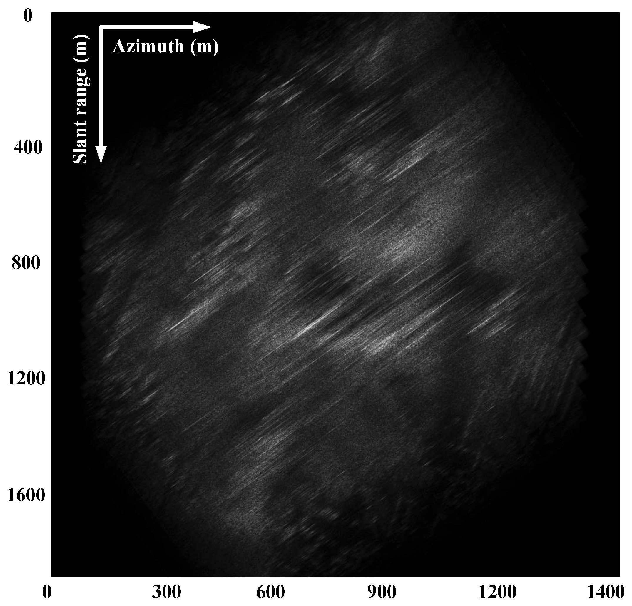
7.2. Raw Data Experiments

In this sub-section, the raw SAR data collected from an airborne platform at a large squint angle of 55 are used to examine the practical performance of the proposed algorithm. The main parameters are the same as in Table 1. As no onboard INU/GPS is available, it is necessary to develop the data-driven auto-calibration approach. Firstly, the raw data are processed by the FFBP, but without motion error compensation, and the imaging result is shown in Figure 11. Due to the unavoidable motion error from the airborne platform deviations, the resultant SAR image encounters severe degradation, where the image is severely blurred and the scene content cannot be distinguished from the SAR image.
By extracting one of dominant scatters within the ground scene, its range-compressed response after FFBP is shown in Figure 12. It is obvious that the range profiles of the scatter shift along with the azimuth samples, which is known as the NsRCM error. It not only causes range defocusing, but also degrades the accuracy of the APE estimation.
Employing the proposed algorithm, a well-focused SAR image is obtained and shown in Figure 13. The image has been transformed into the Cartesian grid. It can be noted that the motion error effects are removed, and a clear ground scene can be seen. Moreover, due to the SAR sensor working in squint mode, the buildings are obvious with the squint shadow in the SAR image.
As the proposed algorithm is capable of correcting not only APE, but also NsRCM error, the range profiles of the dominant scatter are shown in the range-compressed data domain as in Figure 14. It is obvious that the NsRCM error is compensated, and the range shifting is removed.
Similarly to the analysis in the above simulation, the APE function is estimated by WPGA, while the NsRCM error function is obtained by a simple calculation according to Equation (20). The APE and NsRCM error functions used for the error auto-calibration are shown in Figure 15a,b, respectively. Again, due to the FFBP formation, the variation of the NsRCM error function deviates from the APE function, because a derivative term is introduced.
To further evaluate the superiority of the proposed algorithm, the extended ω K algorithm with the motion error compensation is also employed to process the raw data [6,22]. Two representative zoom-in areas are selected from the observed scene (Area 1 and Area 2 in Figure 13) to show the superiority. In Figure 16, the left column gives the zoom-in images processed by the ω K-based motion error compensation [6,22], while the right column shows that processed by the proposed FFBP-based error auto-calibration algorithm. In terms of vision quality, the images by the proposed algorithm have better focusing quality than that by the extended ω K-based algorithm, where a certain extent of smearing can still be observed in the left images, while it is better in the right images. Furthermore, quantitative analysis is also carried out by extracting two dominant scatters, Scatterer 1 and Scatterer 2 from Area 1 and Area 2, respectively. The azimuth responses of Scatterer 1 and Scatterer 2 are plotted in Figure 17a,b, respectively, where the results by the ω K-based algorithm are shown in dashed lines and that by the proposed algorithm are given in solid lines. From the comparisons in Figure 17, the refocused azimuth response by the proposed algorithm has narrower main-lobe and lower sidelobes than that by the ω K-based algorithm. Finally, numerical comparisons in terms of the −3-dB main-lobe, the Peak-Sidelobe Ration (PSLR) and the Integrated Sidelobe Ratio (ISLR) for the focusing quality analysis are listed in Table 2 for the ω -K-based algorithm and Table 3 for the proposed algorithm [12]. Bold labels denote the superior performance of either the ω -K-based algorithm or the proposed algorithm. It is obvious that the proposed algorithm has superior performance in terms of focusing quality (main-lobe resolution and sidelobe level) than the ω -K-based algorithm.

8. Conclusions

In this paper, a novel error auto-calibration algorithm based on FFBP formation is proposed for airborne high-resolution SAR imaging at a large squint angle. The data-driven error auto-calibration algorithm is designed under the FFBP IFP framework, and it avoids complicated processing for the correction of various range migrations. Therefore, the proposed algorithm is capable of forming SAR images without limitations on the squint angle. Moreover, the data-driven error auto-calibration algorithm is implemented in a coherent manner, where both the APE and NsRCM errors are taken into account, and both errors are removed under an analytical and coherent relationship. The relationship is established under the consideration of both errors in the radial and along-track directions, so that it can accommodate the practical SAR data collected at a large squint angle. Both simulated and raw SAR data collected at a high-squint angle are processed to prove the effectiveness of the proposed algorithm, and the resultant performance is compared with the conventional ones to show the superiorities of the proposed algorithm.

Acknowledgments

The work presented in this paper was supported by the National Natural Science Foundation of China under Grant 61601470 and by the Natural Science Foundation of Tianjin, China, under Grant 16JCYBJC41200 (20162898).

Author Contributions

Lei Yang and Song Zhou developed the proposed algorithm, for which Lei Yang specifically organized and wrote the manuscript and Song Zhou conducted the experiments. Lifan Zhao and Mengdao Xing commented on the manuscript and made useful suggestions. Thanks for Renbiao Wu for his helpful suggestions during the revision. Thanks are given for the raw SAR data provided by Xing from Xidian University.

Conflicts of Interest

The authors declare no conflict of interest.

Abbreviations

The following abbreviations are used in this manuscript:
SARSynthetic Aperture Radar
IFPImage Formation Processing
TDBPTime-Domain Back-Projection
FTDBPFast Time-Domain Back-Projection
FFBPFast Factorized Back-Projection
APEAzimuthal Phase Error
NsRCMNon-systematic Range Cell Migration
DPAsDoppler Processing Algorithms
MoCompMotion Compensation
MDMap-Drift
PGAPhase Gradient Autofocusing
MEAMinimum Entropy Autofocusing
WPGAWeighted Phase Gradient Autofocusing
INUInertial Navigation Unit
GPSGlobal Positioning System
PRFPulse Repetition Frequency
UAVUnmanned Aerial Vehicle
PSLRPeak Sidelobe Ratio
ISLRIntegrated Sidelobe Ratio

References

  1. Carrara, W.G.; Goodman, R.S.; Majewski, R.M. Spotlight Synthetic Aperture Radar: Signal Processing Algorithms; Artech House: Norwood, MA, USA, 1995. [Google Scholar]
  2. Cumming, I.G.; Wong, F.H. Digital Signal Processing of Synthetic Aperture Radar Data: Algorithms and Implementation; Artech House: Norwood, MA, USA, 2004. [Google Scholar]
  3. Stroppiana, D.; Azar, R.; Calò, F.; Pepe, A.; Imperatore, P.; Boschetti, M.; Silva, J.M.N.; Brivio, P.A.; Lanari, R. Integration of Optical and SAR Data for Burned Area Mapping in Mediterranean Regions. Remote Sens. 2015, 2, 1320–1345. [Google Scholar] [CrossRef]
  4. Ran, L.; Liu, Z.; Li, T.; Xie, R.; Zhang, L. An Adaptive Fast Factorized Back-Projection Algorithm With Integrated Target Detection Technique for High-Resolution and High-Squint Spotlight SAR Imagery. IEEE J. Sel. Top. Appl. Earth Observ. Remote Sens. 2017, 99, 1–13. [Google Scholar] [CrossRef]
  5. Peng, X.; Wang, Y.; Hong, W.; Wu, Y. Autonomous Navigation Airborne Forward-Looking SAR High Precision Imaging with Combination of Pseudo-Polar Formatting and Overlapped Sub-Aperture Algorithm. Remote Sens. 2013, 11, 6063–6078. [Google Scholar] [CrossRef]
  6. Zhang, L.; Sheng, J.; Xing, M.; Qiao, Z.-J.; Wu, Y.; Bao, Z. Wavenumber-Domain Autofocusing for Highly Squinted UAV SAR Imagery. IEEE Sensors J. 2011, 5, 1574–1588. [Google Scholar] [CrossRef]
  7. Xing, M.; Wu, Y.; Zhang, Y.; Sun, G.C.; Bao, Z. Azimuth Resampling Processing for Highly Squinted Synthetic Aperture Radar Imaging With Several Modes. IEEE Trans. Geosci. Remote Sens. 2014, 7, 4339–4352. [Google Scholar] [CrossRef]
  8. Sun, G.; Jiang, X.; Xing, M.; Qiao, Z.-J.; Wu, Y.; Bao, Z. Focus Improvement of Highly Squinted Data Based on Azimuth Nonlinear Scaling. IEEE Trans. Geosci. Remote Sens. 2011, 6, 2308–2322. [Google Scholar] [CrossRef]
  9. Wu, J.; Xu, Y.; Zhong, X.; Yang, J.M. A Three-Dimensional Localization Method for Multistatic SAR Based on Numerical Range-Doppler Algorithm and Entropy Minimization. Remote Sens. 2017, 9, 470. [Google Scholar] [CrossRef]
  10. Wang, Y.; Li, J.; Xu, F.; Yang, J. A New Nonlinear Chirp Scaling Algorithm for High-Squint High-Resolution SAR Imaging. IEEE Geosci. Remote Sens. Lett. 2017, 12, 2225–2229. [Google Scholar] [CrossRef]
  11. Vandewal, M.; Speck, R.; Suess, H. Efficient and precise processing for squinted spotlight SAR through a modified Stolt mapping. EURASIP J. Adv. Signal Process. 2007, 1, 1–7. [Google Scholar] [CrossRef]
  12. Yang, L.; Zhao, L.; Zhou, S.; Bi, G.; Yang, H. Spectrum-Oriented FFBP Algorithm in Quasi-Polar Grid for SAR Imaging on Maneuvering Platform. IEEE Geosci. Remote Sens. Lett. 2017, 5, 724–728. [Google Scholar] [CrossRef]
  13. Zhou, S.; Yang, L.; Zhao, L.; Bi, G. Quasi-Polar-Based FFBP Algorithm for Miniature UAV SAR Imaging Without Navigational Data. IEEE Trans. Geosci. Remote Sens. 2017, 12, 7053–7065. [Google Scholar] [CrossRef]
  14. Rodriguez, C.M.; Prats, G.; Keieger, G.; Moreira, A. Efficient Time-Domain Image Formation with Precise Topography Accommodation for General Bistatic SAR Configurations. IEEE Trans. Aerosp. Electron. Syst. 2011, 4, 2949–2966. [Google Scholar] [CrossRef] [Green Version]
  15. Ponce, O.; Prats-Iraola, P.; Pinheiro, M.; Rodriguez-Cassola, M.; Scheiber, R.; Reigber, A.; Moreira, A. Fully Polarimetric High-Resolution 3-D Imaging With Circular SAR at L-Band. IEEE Trans. Geosci. Remote Sens. 2014, 6, 3074–3090. [Google Scholar] [CrossRef]
  16. Ulander, L.M.H.; Hellsten, H.; Stenstrom, G. Synthetic-aperture radar processing using fast factorized back-projection. IEEE Trans. Aerosp. Electron. Syst. 2003, 3, 760–776. [Google Scholar] [CrossRef]
  17. Zhang, L.; Li, H.; Qiao, Z.; Xu, Z. A Fast BP Algorithm With Wavenumber Spectrum Fusion for High-Resolution Spotlight SAR Imaging. IEEE Geosci. Remote Sens. Lett. 2014, 9, 1460–1464. [Google Scholar] [CrossRef]
  18. Vu, V.T.; Pettersson, M.I. Nyquist sampling requirements for polar grids in bistatic time-domain algorithms. IEEE Trans. Signal Process. 2015, 2, 457–465. [Google Scholar] [CrossRef]
  19. Zhang, L.; Li, H.; Qiao, Z.; Xing, M.; Bao, Z. Integrating Autofocus Techniques With Fast Factorized Back-Projection for High-Resolution Spotlight SAR Imaging. IEEE Geosci. Remote Sens. Lett. 2013, 6, 1394–1398. [Google Scholar] [CrossRef]
  20. Yegulalp, A.F. Fast backprojection algorithm for synthetic aperture radar. In Proceedings of the 1999 IEEE Radar Conference on Radar into the Next Millennium, Waltham, MA, USA, 22 April 1999; pp. 60–65. [Google Scholar]
  21. Yang, L.; Xing, M.; Wang, Y.; Zhang, L.; Bao, Z. Compensation for the NsRCM and Phase Error After Polar Format Resampling for Airborne Spotlight SAR Raw Data of High Resolution. IEEE Geosci. Remote Sens. Lett. 2013, 1, 165–169. [Google Scholar] [CrossRef]
  22. Xu, G.; Xing, M.; Zhang, L.; Bao, Z. Robust Autofocusing Approach for Highly Squinted SAR Imagery Using the Extended Wavenumber Algorithm. IEEE Trans. Geosci. Remote Sens. 2013, 10, 5031–5046. [Google Scholar] [CrossRef]
  23. Zhang, L.; Li, H.; Xu, Z.; Wang, H.; Yang, L.; Bao, Z. Application of fast factorized back-projection algorithm for high-resolution highly squinted airborne SAR imaging. Sci. China 2017, 6, 1–17. [Google Scholar] [CrossRef]
  24. Zhang, L.; Qiao, Z.; Xing, M.; Yang, L.; Bao, Z. A Robust Motion Compensation Approach for UAV SAR Imagery. IEEE Trans. Geosci. Remote Sens. 2012, 8, 3202–3218. [Google Scholar] [CrossRef]
  25. Xing, M.; Jiang, X.; Wu, R.; Zhou, F.; Bao, Z. Motion compensation for UAV SAR based on raw radar data. IEEE Trans. Geosci. Remote Sens. 2009, 8, 2870–2883. [Google Scholar] [CrossRef]
  26. Yang, L.; Xing, M.; Zhang, L.; Sheng, J.; Bao, Z. Entropy-based motion error correction for high-resolution spotlight SAR imagery. IET Radar Sonar Navig. 2012, 7, 627–637. [Google Scholar] [CrossRef]
Figure 1. Squint SAR geometry in the slant-range plane.
Remotesensing 10 00321 g001
Figure 2. FFBP recursion.
Remotesensing 10 00321 g002
Figure 3. Processing flowchart of the proposed algorithm.
Remotesensing 10 00321 g003
Figure 4. Simulated squint SAR geometry.
Remotesensing 10 00321 g004
Figure 5. Simulated motion errors in the (a) radial direction and (b) along-track direction.
Remotesensing 10 00321 g005
Figure 6. 3D response of the (a) center scatter and (b) edge scatter without motion error compensation.
Remotesensing 10 00321 g006
Figure 7. Estimated (a) APE error function and calculated (b) NsRCM error function for compensation.
Remotesensing 10 00321 g007
Figure 8. 3D response of the (a) center scatter and (b) edge scatter after the proposed motion error compensation.
Remotesensing 10 00321 g008
Figure 9. Azimuth response comparison of (a) the center scatter and (b) the edge scatter processed by the proposed FFBP-based motion compensation (solid lines) and the ω K-based motion compensation (dashed lines).
Remotesensing 10 00321 g009
Figure 10. Focused SAR image of all 9 simulated point scatters.
Remotesensing 10 00321 g010
Figure 11. Squint SAR image without motion error compensation.
Remotesensing 10 00321 g011
Figure 12. Range profiles without motion error compensation.
Remotesensing 10 00321 g012
Figure 13. Squint SAR image with the proposed error auto-calibration.
Remotesensing 10 00321 g013
Figure 14. Range profiles with the proposed NsRCM correction.
Remotesensing 10 00321 g014
Figure 15. (a) Estimated APE function and (b) calculated NsRCM error function.
Remotesensing 10 00321 g015
Figure 16. Comparison of zoom-in SAR image by the ω K-based MoComp algorithm (left images) and the proposed algorithm (right images).
Remotesensing 10 00321 g016
Figure 17. (a) Azimuth response comparison of Scatterer 1 in Area 1 and (b) azimuth response comparison of Scatterer 2 in Area 2.
Remotesensing 10 00321 g017
Table 1. Simulated parameters of airborne squint SAR.
Parameters
Centroid FrequencyX-Band
Bandwidth180 MHz
Sampling rate200 MHz
PRF600 Hz
Reference Range17 km
Velocity∼132 m/s
Squint Angle∼55°
Table 2. Focusing quality of the ω K-based MoComp algorithm.
Range Direction
3-dB widthPSLRISLR
Scatterer 10.92 m−27.32 dB−23.75 dB
Scatterer 20.96 m−26.48 dB−24.63 dB
Azimuth direction
3-dB widthPSLRISLR
Scatterer 10.90 m−15.23 dB−13.39 dB
Scatterer 20.81 m−25.02 dB−10.62 dB
Table 3. Focusing quality of the proposed algorithm.
Range Direction
3-dB widthPSLRISLR
Scatterer 10.91 m−30.62 dB−27.13 dB
Scatterer 20.92 m−29.11 dB−26.04 dB
Azimuth direction
3-dB widthPSLRISLR
Scatterer 10.72 m−24.87 dB−21.59 dB
Scatterer 20.75 m−17.75 dB−16.32 dB

