Estimating Uncertainty of Point-Cloud Based Single-Tree Segmentation with Ensemble Based Filtering

1
Geographic Information Systems Laboratory, Ecole Polytechnique Fédérale de Lausanne, 1015 Lausanne, Switzerland
2
Laboratory of Geo-information Science and Remote Sensing, Wageningen University, 6708 PB Wageningen, The Netherlands
*
Author to whom correspondence should be addressed.
Remote Sens. 2018, 10(2), 335; https://doi.org/10.3390/rs10020335
Submission received: 14 November 2017
/
Revised: 9 February 2018
/
Accepted: 21 February 2018
/
Published: 23 February 2018
(This article belongs to the Special Issue Lidar for Forest Science and Management)
Abstract
:Individual tree crown segmentation from Airborne Laser Scanning data is a nodal problem in forest remote sensing. Focusing on single layered spruce and fir dominated coniferous forests, this article addresses the problem of directly estimating 3D segment shape uncertainty (i.e., without field/reference surveys), using a probabilistic approach. First, a coarse segmentation (marker controlled watershed) is applied. Then, the 3D alpha hull and several descriptors are computed for each segment. Based on these descriptors, the alpha hulls are grouped to form ensembles (i.e., groups of similar tree shapes). By examining how frequently regions of a shape occur within an ensemble, it is possible to assign a shape probability to each point within a segment. The shape probability can subsequently be thresholded to obtain improved (filtered) tree segments. Results indicate this approach can be used to produce segmentation reliability maps. A comparison to manually segmented tree crowns also indicates that the approach is able to produce more reliable tree shapes than the initial (unfiltered) segmentation.
1. Introduction
Airborne Laser Scanning (ALS) is an effective technology to support forest survey, research and management [1,2,3]. ALS can provide valuable data on forest structure and composition, in the form of dense 3D point clouds which can be further processed to create a range of useful products (such as topographical relief, canopy height, canopy layering, timber volume, canopy fuel characteristics, stand/edge delineation and deciduous/coniferous proportion).
Individual Tree Crown (ITC) segmentation from ALS data is a nodal problem in forest remote sensing and many different algorithms have been proposed to address it [4,5,6,7,8]. Errors in individual tree shape delineation propagate in further processing steps (e.g., timber volume, biomass and species prediction), so it is important to quantify them. However, the majority of segmentation algorithms do not directly provide any information about shape delineation uncertainty. Instead, the evaluation of shape delineation accuracy is usually done by comparing the segmentation with an independently produced and reliable reference (e.g., manual segmentation and/or field surveys). However, this approach is limited by the low availability of individual tree shape reference data over large areas. For this reason, 3D shape delineation accuracy is very often not evaluated in ITC segmentation studies [9]. Even though independent tree shape validation data may not be available, quantifying segmentation uncertainty is still necessary. One possible solution is to use algorithms which compare observed values with model based expectations (geostatistics, for example, model spatial autocorrelation as function of range). In addition to providing a prediction uncertainty, these methods also typically produce better predictions, because they incorporate prior knowledge about the investigated phenomenon. In the context of ITC segmentation, such approaches involve modeling the spatial distribution and/or the shape of trees based on prior botanical and ecological knowledge. Many tree species exhibit an increase in crown geometry variability (heteroscedasticity) as a function of age (height) and environmental conditions. However, some coniferous species (such as Spruce and Fir) exhibit less geometric variability and are generally easier to model. For this reason, model based segmentation algorithms are generally better suited for coniferous forests. Several model based segmentation approaches have been proposed. Swetnam et al. [10] incorporate an allometric model based on the metabolic scaling theory into a tree detection algorithm, to improve detection rates and accuracy. Similarly, Sačkov et al. [11] use empirical allometric relations between tree height and crown radius, horizontal/vertical spacing rules and height difference criteria to separate adjacent tree crowns. Pouliot et al. [12], Heinzel et al. [13] and Ene et al. [14] use crown model dependent rules to locally optimize segmentation parameters. They locally adjust raster Canopy Height Model (CHM) spatial resolutions, levels of Gaussian (low pass filter) smoothing or local maxima search radius (for tree top detection). Pirotti [15] and Holmgren et al. [16] both use a template (based on crown radius-height ratio relations) matching approach to detect trees and avoid undersegmentation. Andersen et al. [17] and Lähivaara et al. [18] use a simple solid of revolution (ellipsoid) model to approximate different tree shapes. Using the Bayesian statistical framework, they then determine an optimal fit (i.e location and shape parameters) by estimating the model parameters for each tree. Zhang et al. [19] optimize a stochastic model which includes both the spatial distribution and the tree shape (with crown radial symmetry and area criteria). Although they do not focus on model based segmentation, Ko et al. [20] propose an indirect method to assign a segmentation quality index to ITC segments. They first perform a supervised classification (Random Forest) of tree genera based on geometric features derived from the ITC segments. Then, they assign a quality index to the ITC segments based on their class ambiguity (correct classification rate).
In this article, a method which models tree shape probability directly from the ALS data (i.e., without the need for a predefined model) is proposed. The method uses the ensemble learning (model averaging) framework [21,22,23]. An ensemble is a group of segments which share similar (geometric and radiometric) features. We make the hypothesis that segments in an ensemble can be considered as noisy instances of the same tree shape template. By comparing all shape instances within an ensemble, inconsistencies between the shapes can be detected and an estimate of a probable underlying tree shape is obtained. The proposed method depends on several assumptions:
- Tree top geometric features can be used as proxies of overall tree shape.
- Tree crowns exhibit approximate radial symmetry.
- Tree growth is approximately vertical.
Under these assumptions, the approach is mainly suitable for coniferous forests. The goals of this paper are: First, to develop a method to estimate ITC segmentation uncertainty at the point level that does not rely on validation data. Second, to evaluate how removing points with different degrees of uncertainty influences the 3D shape delineation quality of the trees.
The following sections present the data and explain the method. The results are then evaluated and discussed.
2. Materials
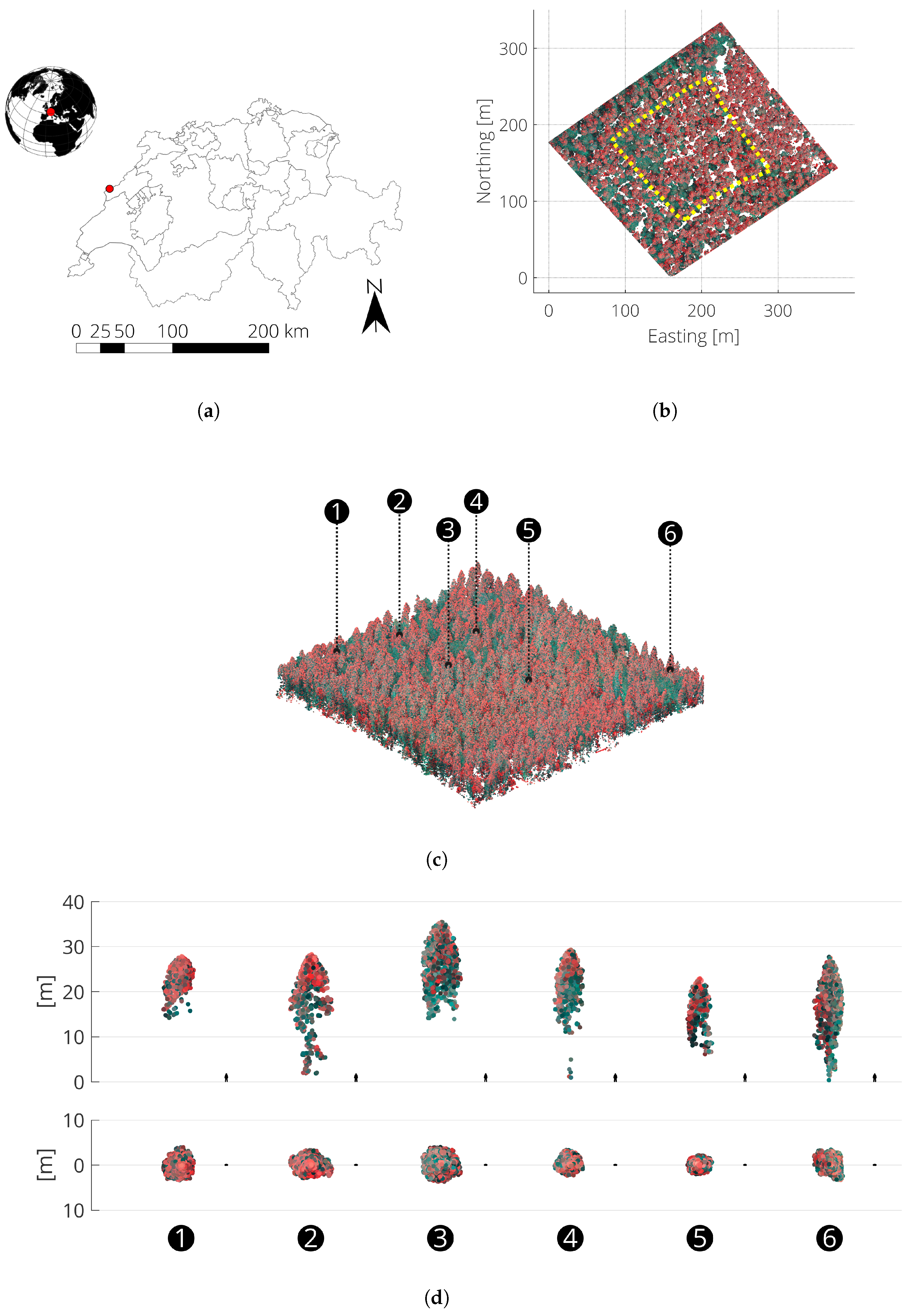
The method was tested on a site (cf. Figure 1a) located in northwest Switzerland (46.96035 N, 6.50852 E, 1150 m a.s.l). The site is a uneven-aged coniferous dominated forest plot of ~5 ha. The central 1.97 ha part of the plot (yellow polygon in Figure 1b) was inventoried with measurement of approximate tree location, Diameter at Breast Height (DBH) and species by the Neuchâtel forest service, in October 2015. Results derived from this field inventory are reported in Table 1.
ALS data was acquired simultaneously (i.e., camera and LiDAR system mounted on the same aircraft) with aerial imagery between March and May 2016 over the State of Neuchâtel. The data used in this study is a subset of the state-wide acquisition. The acquisition metadata (for the study areas) is presented in Table 2 and the point cloud covering the study site is illustrated in Figure 1b.
The return intensity was normalized (by the data provider) with respect to the sensor to surface range using the formula described in [24]:
where:
- is the normalized intensity;
- I is the raw intensity;
- r is the range between the sensor and the point;
- is an arbitrary constant reference range (1000 m was used here).
Using a custom built (Matlab based) application, the 3D tree shapes were manually delineated in the point cloud to produce a set of reference segments (cf. Figure 1d). The shape delineation process involved extracting subsets of the point cloud, visualizing them under different viewing angles and progressively removing points until a single tree was visible. In cases where trees were in very close proximity, horizontal cross sections were also used to separate adjacent crowns. Segments with an ambiguous shape (e.g., when there was a suspicion of the presence of multiple trees in a segment) were flagged and excluded from the validation dataset. The resulting reference dataset contained a total of 940 tree segments (754 coniferous, 122 deciduous and 64 unidentified or dead trees). These reference samples include a variability of height (age) and shape. Only the coniferous trees were used for validation.
In this study, the ensembles were built using data covering the study site and two additional sites in the same region. Three criteria are important when selecting/preparing data to build ensembles:
- Most of the tree shape variability for the species (spruce and fir here) and heights of interest should be covered.
- It is expected that the reliability of the average shape estimation increases with the number of observations. So, multiple examples of the same tree shape should be available to ensure an ensemble size that allows determination of the average shape unambiguously.
- If radiometric features are used to build the ensembles, all sample areas should be in the same phenological stage and echo intensity must be rescaled to a common range.
3. Methods
3.1. Overview
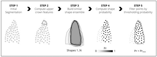
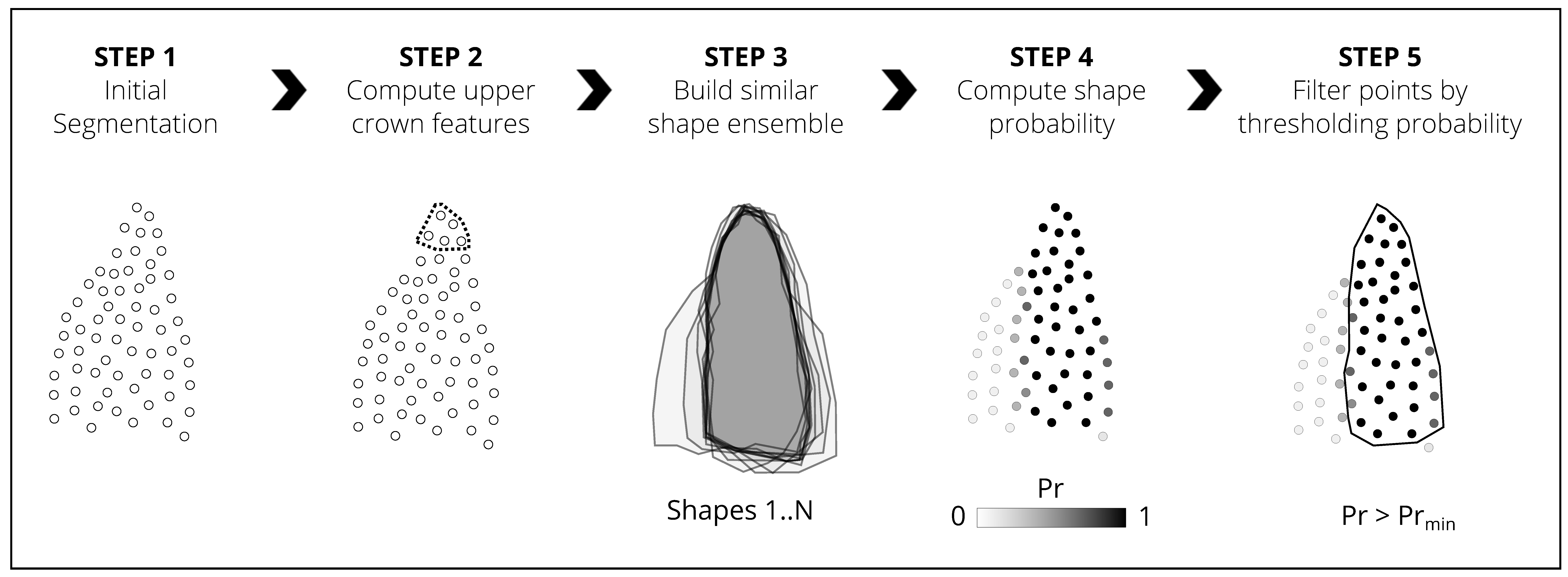
The proposed workflow starts with a set of ITC segments (obtained with any generic segmentation algorithm, such as marker controlled watershed [25,26,27]). Each segment is then characterized by a set of descriptive (geometric and radiometric) features and matched with similar segments to form ensembles (groups). Within each ensemble, the 3D alpha shapes (concave hulls) [28] derived from the point cloud segments are mutually overlaid to detect common regions and determine shape probability. A threshold is then applied to the probability, to filter out erroneous points from the initial segmentation.
3.2. Step 1-Initial Segmentation
A 0.4 m resolution raster Canopy Height Model (CHM) is first derived from the classified 3D point clouds (for the three sample sites). The CHM is smoothed using a Gaussian 6 × 6 lowpass filter. Tree top (local maxima) detection is then performed using a variable radius (r) convolution window defined by a function of the pixel metric height (h):
The local maxima are merged and the highest point is retained, if separated by less than the 3D adjacency distance defined by function :
The choice of a logarithmic variable radius in Equations (2) and (3) is based on the observed relationship between upper crown radius and tree height in the region of interest. However, this relationship may vary significantly between forest types [30] and other variable radius functions such as those proposed in [31,32,33] may be used in place of Equations (2) and (3) .
The detected local maxima (cf. Figure 3a) are subsequently used as markers (i.e., seed points) in watershed segmentation [25,26,27] to label individual tree crowns (cf. Figure 3b). The CHM labels are then assigned to their nearest 3D points, to obtain a 3D labeled point cloud. The presence of partial tree crowns would bias the shape probability estimates. Thus, segments located within 10 m of the edge of the point cloud are excluded. For the same reason, the segmentation parameter values (regardless of the segmentation algorithm) should be set to avoid over-segmentation.
3.3. Step 2-Computing Upper Crown Features
In order to compare and group tree shapes in step 3, a set of descriptive features is required. Thus, the total height h, upper crown (i.e., points located in the upper 15% of the crown) convex volume v and median return intensity i (normalized by the [0.05, 0.95] quantile range) are computed for each segment. These upper crown features were chosen because for trees with a conical shape, they are less affected by poor segmentation than features that describe the lower parts of segments (cf. Figure 4a).
3.4. Step 3-Building Shape Ensembles (Grouping Similar Segments)
First, the XYZ point coordinates of each segment i are normalized so that the segment origin is vertically aligned with the tree top:
where:
- N is the number of points in segment i;
- is a N × 3 matrix containing the normalized 3D point coordinates of segment i;
- is a N × 3 matrix containing the original 3D point coordinates of segment i;
- is a 1 × 3 matrix containing the root coordinate of the segment i (i.e., the projection of the tree top on the terrain model);
- is a N × 1 vector of ones.
This coordinate normalization is required to overlay (stack) all shapes within an ensemble. Then, the single region 3D alpha shape [28] (cf. Figure 4b) of each segment is computed and any holes in the shape are filled. Subsequently, ensembles (cf. Figure 5) are constructed by grouping segments which share similar geometric and radiometric features (computed at step 2). Formally, given a segment i with total height , upper crown convex volume and upper crown median intensity , all segments j with which fulfill the criteria listed in Table 3 form the ensemble i.
The tolerances in terms of height, upper crown volume and median intensity differences used when matching segments are set empirically. There is a trade-off between these margins and the ensemble sizes. Tighter tolerances result in smaller ensembles and thus larger datasets are needed to reach the minimum required ensemble sizes.
3.5. Step 4-Computing Shape Probability
The shape probability is defined as the number of times a point was included in the alpha shapes of the ensemble divided by the ensemble size N (i.e., number of matching segments), as illustrated in Figure 6. For each set of points which form a segment, the shape probability is given by:
where:
- is the alpha shape of segment i;
- is the set of N alpha shapes with features similar to ;
- N is the number of segments in the ensemble i;
- is the minimum number of segments per ensemble required to compute a reliable shape probability (10 was used here).
Thus, regions which are common to many alpha shapes in the ensemble obtain higher probability scores than regions that are only visible in few segments.
3.6. Step 5-Filtering
The points from the initial segments can be filtered by applying a threshold () to the shape probability. The filtered point subset is defined by:
where:
- is the indicator function which produces the filtered point subset;
- is the shape probability associated with each point in segment i;
- is the minimum probability required to retain a point in the segment.
An optimal value of can be set by visually examining the effect of applying different threshold values to a (height stratified) sample of the segments.
4. Results
In this section, we apply the proposed method to the described study site and evaluate its performance in terms of tree detection rate and 3D shape delineation accuracy.
4.1. Validation Metrics
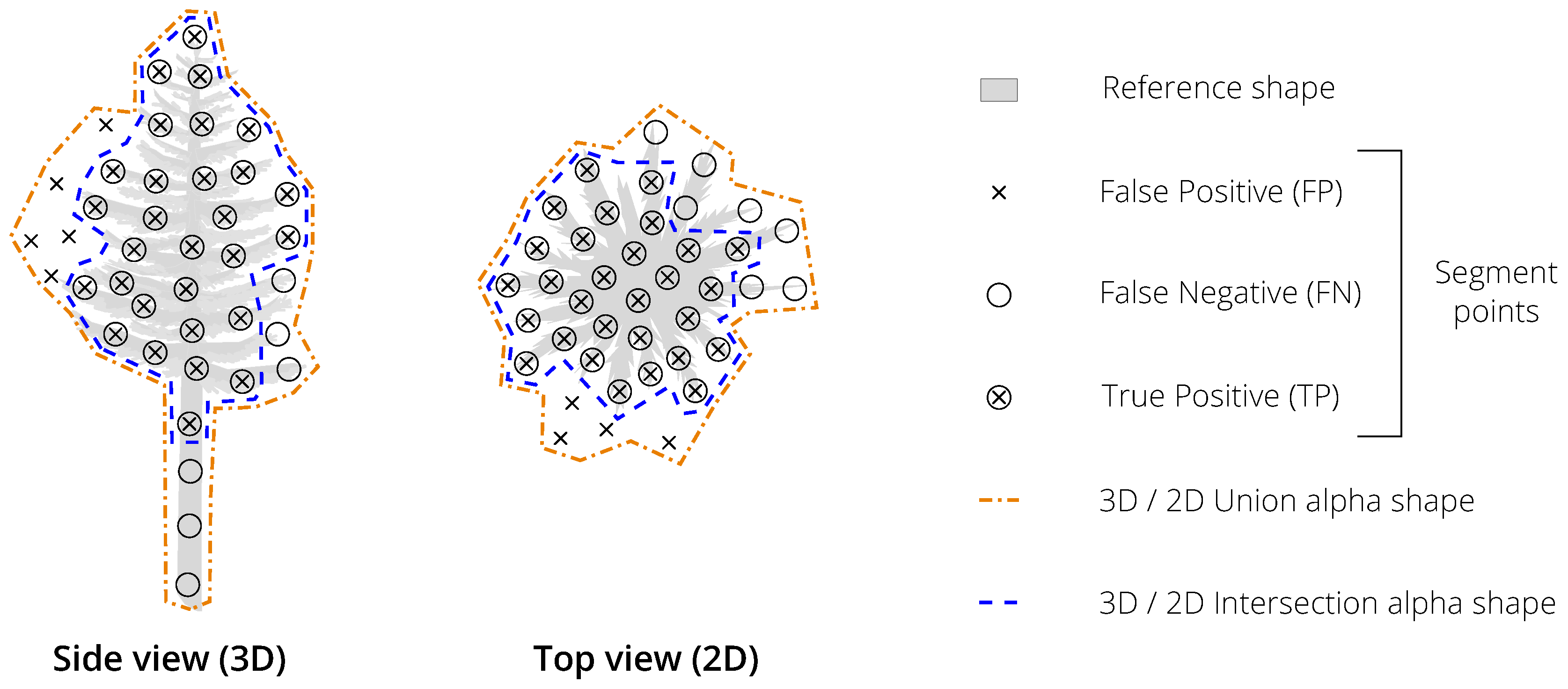
The unfiltered (initial) and filtered shapes were compared to the manually delineated reference shapes. The delineation performance (cf. Figure 7) was evaluated (for detected trees only) in terms of recall r (Equation (7)), precision p (Equation (8)), F-score F (Equation (9)) and Intersection over Union . The IoU metric was applied to assess the point pattern overlap (Equation (10)), the volumetric (3D) overlap (Equation (11)) and the horizontal areal (2D) overlap (Equation (12)). is defined as the ratio of the intersection 3D alpha shape volume over the union 3D alpha shape volume (cf. Figure 7). The value of is set by computing the single region alpha shape of the union point set. The same value is subsequently used when computing the intersection alpha shape. Similarly, is defined as the ratio of the intersection 2D alpha shape area over the union 2D alpha shape area (cf. Figure 7). The correct detection rate (d) was computed as the proportion of segments with a delineation > 0.5 (i.e., a segment is considered to be detected if more than half of its points overlap with the reference points).
Recall indicates if the delineation tends to include all the tree points, precision indicates the fraction of included points that are correct and F score is a composite (harmonic mean) of both metrics. The pointwise (), volumewise () and areawise () IoU scores indicate how well the tested shape overlaps with the reference shape. The volumewise IoU () and areawise IoU () are sensitive to the spatial point distribution (which defines the shape) while the pointwise IoU () is more sensitive to the number of overlapping points.
4.2. Performance
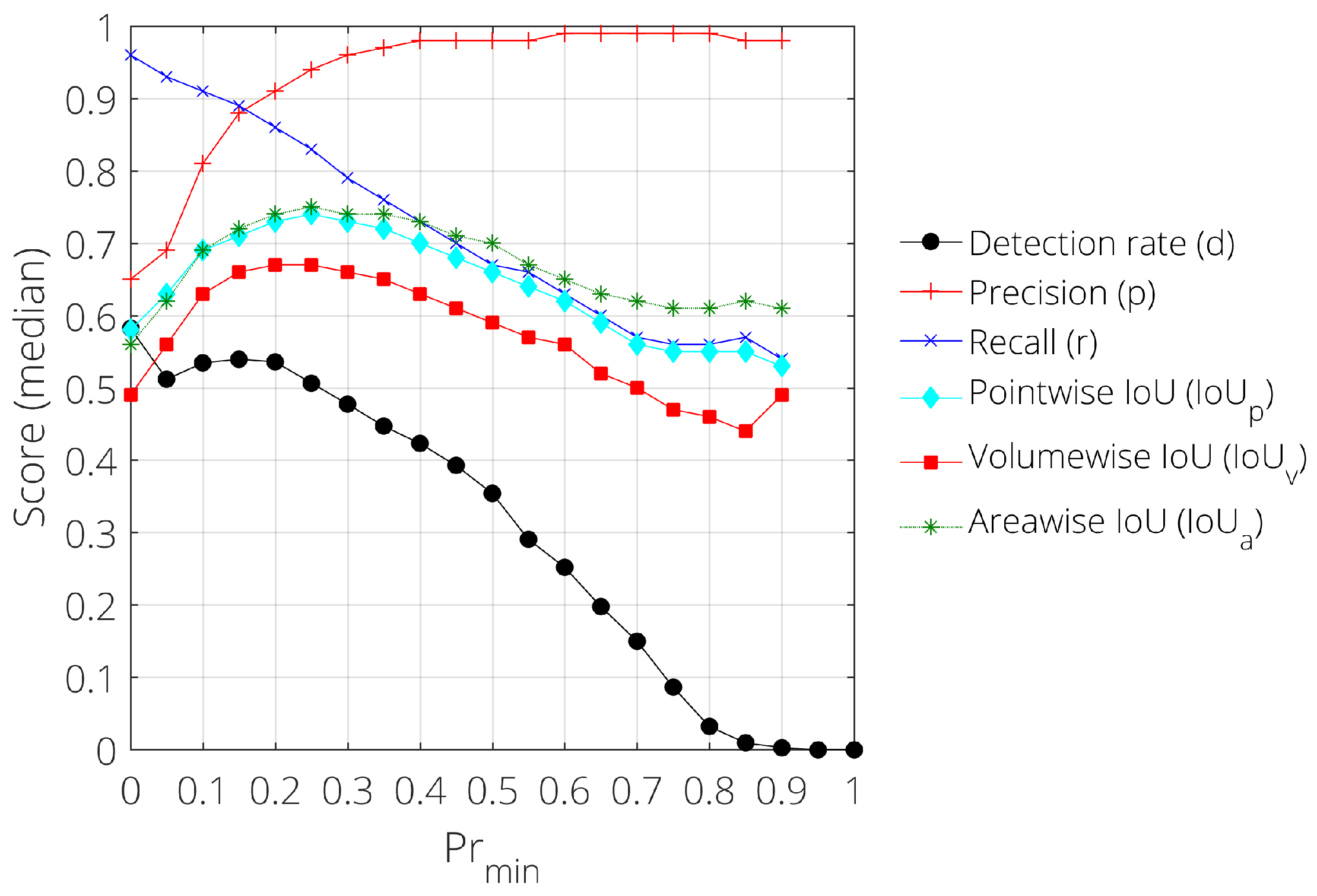
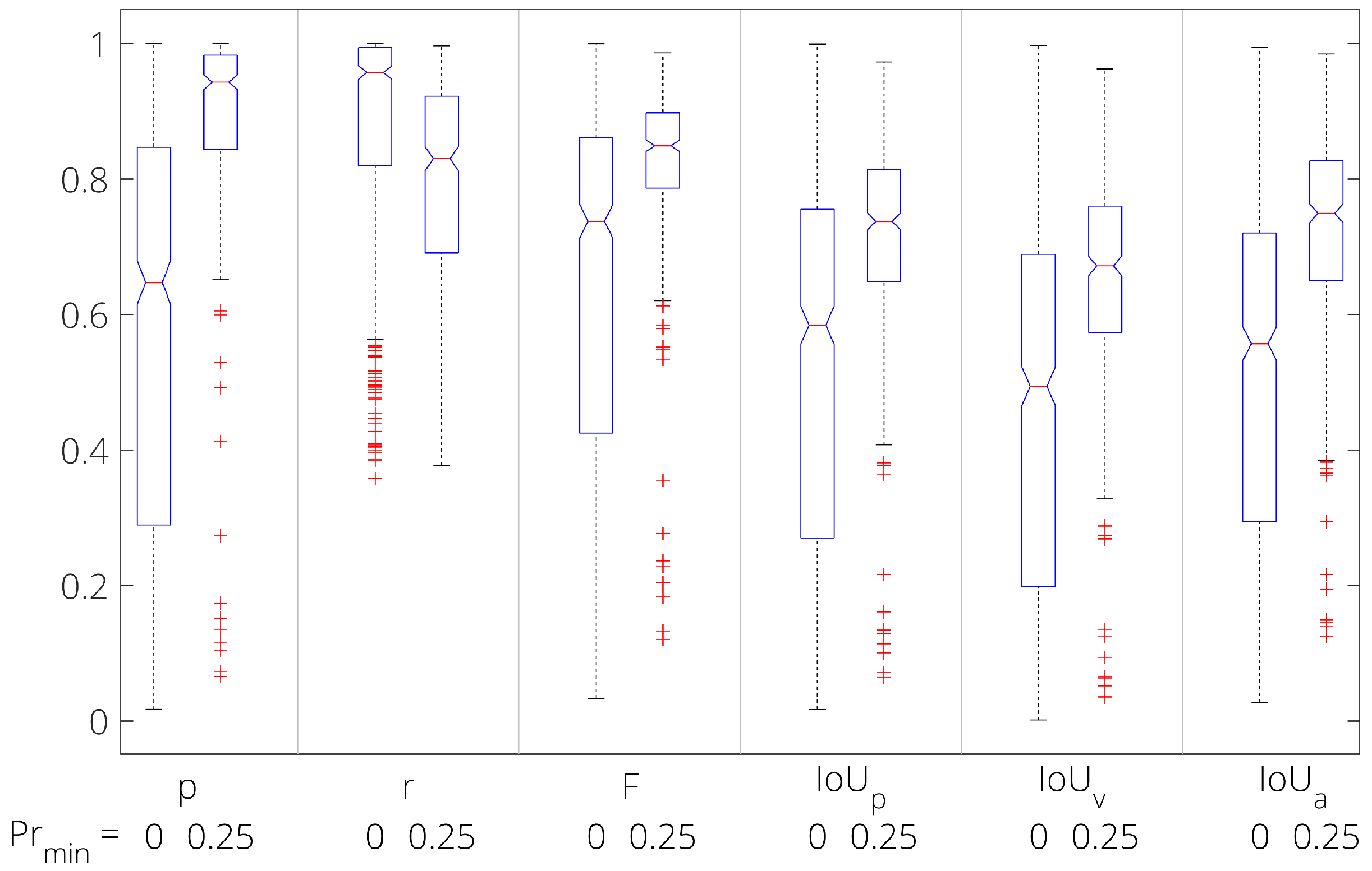
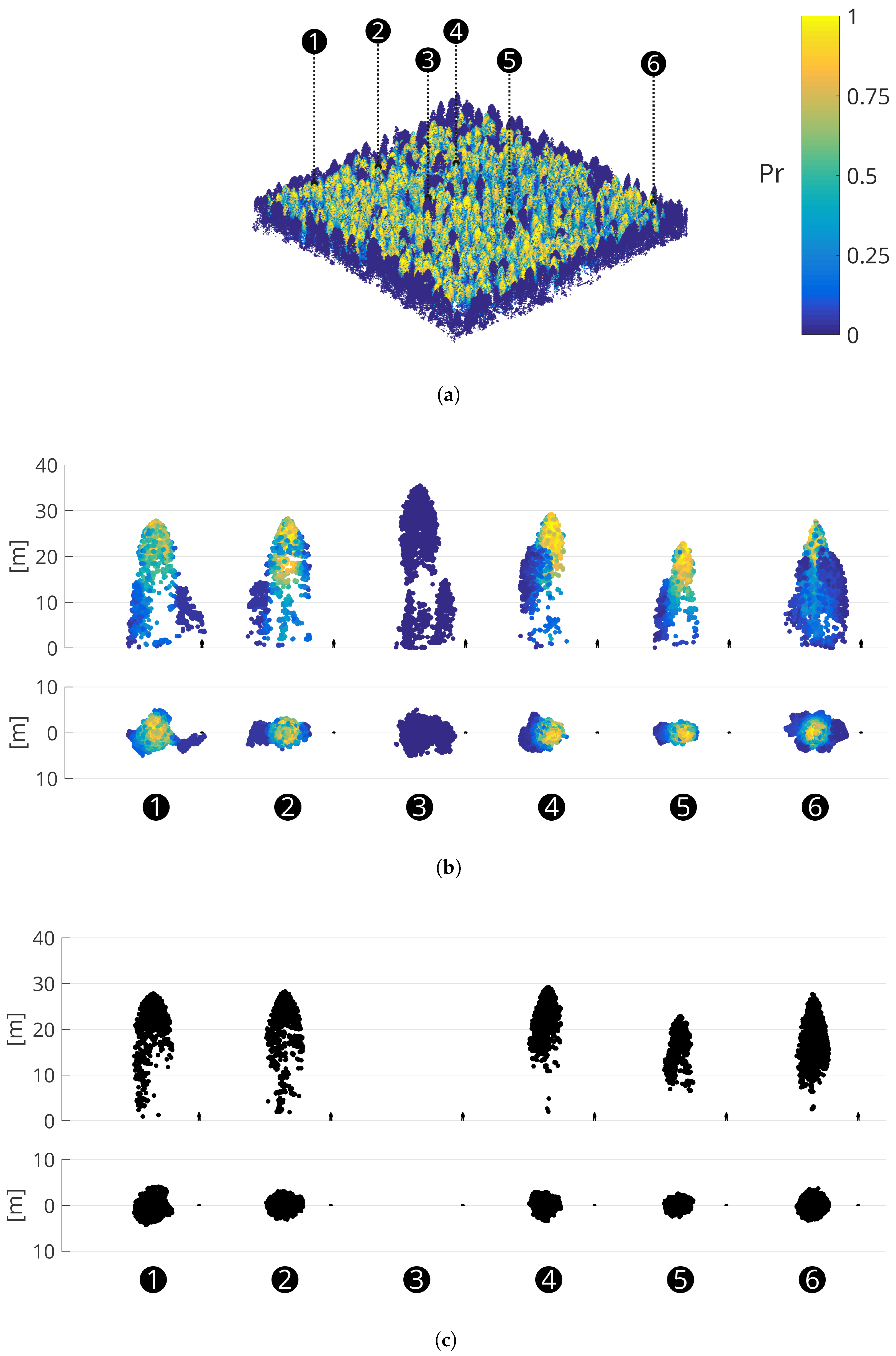
The detection metric and the median of each delineation metric (except F score) for different values of are presented in Figure 8. The same metrics for are also reported in Table 4 stratified by height category. Figure 9 provides boxplots of the delineation metrics. Figure 10a illustrates the resulting probability map, Figure 10b provides examples of individual tree shape probability and Figure 10c shows the resulting filtered segments.
A one-sided Wilcoxon signed-rank test was used to compare the delineation before and after filtering with . This test was chosen because the before/after delineation scores are dependent and not normally distributed. In this test, the alternate hypothesis is that the score values after filtering minus those before filtering come from a distribution with a median greater than 0. Using a 0.5% (i.e., ) significance level, the alternate hypothesis was accepted for all the delineation scores except recall. In other words, these delineation scores were significantly higher after filtering. The associated p-values of the comparison tests were p: , r: 1, F: , : , : , : .
5. Discussion
The results indicate that the proposed method can produce an estimate of tree shape delineation uncertainty. Shape probability at the point scale can be aggregated at the segment scale to produce a mean or median shape probability providing information on individual segment shape uncertainty.
In the presented study case, when using values ranging from 0.1 to 0.6, the IoU scores are improved with a peak at . The precision score is increased and the recall score is reduced for all values of . The detection rate is also reduced for all values of . This reduction in detection rate is due to the definition which requires for a segment to be counted as a correct detection. The better delineation scores obtained after filtering are due to the combined effect of removing erroneous points and discarding segments with .
For practical applications over large areas, it is sufficient to compute ensembles based on a subset of the area which includes most of the tree shape variability and a sufficient amount of redundant shape examples. By thresholding the resulting shape probability, a set of tree shape templates are produced. New segments (i.e., outside the sample area) can then be matched (i.e., using upper crown features) and compared with their most similar shape template to produce an estimate of their segmentation uncertainty.
The proposed ensemble based filtering method has several advantages. The segmentation/shape uncertainty estimate can be improved by adding additional observations to the ensembles. The method is adaptive because it does not rely on predefined allometric rules or 3D model templates. Moreover, although marker controlled watershed was used to produce the segmentation, any other automatic or manually delineated segments could be used instead in the first step. Finally, the method does not require high ALS point densities.
The main drawbacks of the method are its dependency on specific coniferous tree shapes, the need to use datasets with multiple examples of similar trees and the computational cost. Most of the computation time is used to compute the single region alpha shapes (~23%) and the shape probability inclusion tests (~74%). The total time to apply the method for the three sites used in this study was ~30 min. This computation time may be reduced by sub-sampling the point cloud (i.e., lowering density) and using fixed values of when computing the alpha shapes.
Further improvements could involve classification and separation of deciduous and coniferous trees, before running the algorithm. This separation step could be accomplished using ALS data alone using intensity (leaf-off), opacity (leaf-off) and/or shape features, for example with the approach described in [34]. The method is conditioned by the segmentation algorithm employed in step 1. In the current implementation, marker controlled watershed segmentation is used, thus points located in crown intersection regions cannot be allocated to a tree with certainty. This limitation could be improved by using a more sophisticated segmentation algorithm working at the inner crown level. Additional features could be included to improve the segment grouping step. These could include RGB or multispectral indices (e.g., from multiple wavelength LiDAR), geometric features (e.g., crown base height, convexity, surface area, projected area, etc.). In particular, the addition of crown base height (which can be estimated for example with the approach used in [35]) to the list of grouping features used at step 3 could possibly improve the shape uncertainty estimate beneath the crown base. In addition, since it is assumed that coniferous trees exhibit approximate vertical radial symmetry, additional shape instances could be generated artificially by simply rotating the segments around the vertical (Z) axis. Finally, the alignment of segments could be improved by using a more elaborated co-registration algorithm. The segmentation and filtering procedure could theoretically be repeated and detected trees removed at each iteration until no more detectable trees were left in the point cloud. Finally, the method may also be employed to automatically create 3D tree shape templates which can be used in other processing routines.
6. Conclusions
When working at the individual tree scale, knowing which tree segments are reliable is fundamental to correctly interpret derived characteristics (e.g., diameter, biomass, species). However, the problem of directly estimating ITC shape segmentation error (outside validation areas) has not been thoroughly addressed by the forest remote sensing community. In this article, we have studied how the ensemble learning framework can be used to estimate shape probability at the point level for coniferous forests (spruce and fir). Based on this shape probability, it was shown that a range of minimum probability thresholds can be applied to filter the initial segmentation and produce more reliable tree shapes.
Acknowledgments
The authors would like to thank Marc Riedo from the state of Neuchâtel (Switzerland) for providing the ALS data and Pascal Junod of the Neuchâtel Forest Service/Sylviculture Competence Center (CCS, http://www.waldbau-sylviculture.ch) for providing field inventory data. The authors would also like to thank the four anonymous reviewers for their comments. This research was supported by the Swiss Forestry and Wood Research Fund (project 2013.18). D.T is supported by the Swiss National Science Foundation (grant PZ00P2-136827, http://p3.snf.ch/project-136827).
Author Contributions
M.P. conceived and evaluated the method, wrote the paper. D.T. reviewed the manuscript and provided technical and layout advice.
Conflicts of Interest
The authors declare no conflict of interest.
Abbreviations
The following abbreviations are used in this manuscript:
| ALS | Airborne Laser Scanning |
| CHM | Canopy Height Model |
| DBH | Diameter at Breast Height |
| FN | False Negative |
| FP | False Positive |
| GNSS | Global Navigation Satellite System |
| IoU | Intersection over Union |
| ITC | Individual Tree Crown |
| RGB | Red-Green-Blue |
| TIN | Triangular Irregular Network |
| TP | True Positive |
References
- Maltamo, M.; Næsset, E.; Vauhkonen, J. (Eds.) Forestry Applications of Airborne Laser Scanning. In Managing Forest Ecosystems; Springer: Dordrecht, The Netherlands, 2014; Volume 27. [Google Scholar]
- Waser, L.T.; Boesch, R.; Wang, Z.; Ginzler, C. Towards Automated Forest Mapping. In Mapping Forest Landscape Patterns; Springer: New York, NY, USA, 2017; pp. 263–304. [Google Scholar]
- Wulder, M.A.; White, J.C.; Nelson, R.F.; Næsset, E.; Ørka, H.O.; Coops, N.C.; Hilker, T.; Bater, C.W.; Gobakken, T. Lidar Sampling for Large-Area Forest Characterization: A Review. Remote Sens. Environ. 2012, 121, 196–209. [Google Scholar] [CrossRef]
- Wang, Y.; Hyyppä, J.; Liang, X.; Kaartinen, H.; Yu, X.; Lindberg, E.; Holmgren, J.; Qin, Y.; Mallet, C.; Ferraz, A.; et al. International Benchmarking of the Individual Tree Detection Methods for Modeling 3-D Canopy Structure for Silviculture and Forest Ecology Using Airborne Laser Scanning. IEEE Trans. Geosci. Remote Sens. 2016, 54, 5011–5027. [Google Scholar] [CrossRef]
- Zhen, Z.; Quackenbush, L.J.; Zhang, L. Trends in Automatic Individual Tree Crown Detection and Delineation—Evolution of LiDAR Data. Remote Sens. 2016, 8, 333. [Google Scholar] [CrossRef]
- Eysn, L.; Hollaus, M.; Lindberg, E.; Berger, F.; Monnet, J.M.; Dalponte, M.; Kobal, M.; Pellegrini, M.; Lingua, E.; Mongus, D.; Pfeifer, N. A Benchmark of Lidar-Based Single Tree Detection Methods Using Heterogeneous Forest Data from the Alpine Space. Forests 2015, 6, 1721–1747. [Google Scholar] [CrossRef] [Green Version]
- Vauhkonen, J.; Ene, L.; Gupta, S.; Heinzel, J.; Holmgren, J.; Pitkänen, J.; Solberg, S.; Wang, Y.; Weinacker, H.; Hauglin, K.M.; et al. Comparative Testing of Single-Tree Detection Algorithms under Different Types of Forest. For. Int. J. For. Res. 2012, 85, 27–40. [Google Scholar] [CrossRef]
- Kaartinen, H.; Hyyppä, J.; Yu, X.; Vastaranta, M.; Hyyppä, H.; Kukko, A.; Holopainen, M.; Heipke, C.; Hirschmugl, M.; Morsdorf, F.; et al. An International Comparison of Individual Tree Detection and Extraction Using Airborne Laser Scanning. Remote Sens. 2012, 4, 950–974. [Google Scholar] [CrossRef] [Green Version]
- Yin, D.; Wang, L. How to Assess the Accuracy of the Individual Tree-Based Forest Inventory Derived from Remotely Sensed Data: A Review. Int. J. Remote Sens. 2016, 37, 4521–4553. [Google Scholar] [CrossRef]
- Swetnam, T.L.; Falk, D.A. Application of Metabolic Scaling Theory to Reduce Error in Local Maxima Tree Segmentation from Aerial LiDAR. For. Ecol. Manag. 2014, 323, 158–167. [Google Scholar] [CrossRef]
- Sačkov, I.; Hlásny, T.; Bucha, T.; Juriš, M. Integration of Tree Allometry Rules to Treetops Detection and Tree Crowns Delineation Using Airborne Lidar Data. iFor. Biogeosci. For. 2017, 10, 459. [Google Scholar] [CrossRef]
- Pouliot, D.; King, D. Approaches for Optimal Automated Individual Tree Crown Detection in Regenerating Coniferous Forests. Can. J. Remote Sens. 2005, 31, 255–267. [Google Scholar] [CrossRef]
- Heinzel, J.N.; Weinacker, H.; Koch, B. Prior-Knowledge-Based Single-Tree Extraction. Int. J. Remote Sens. 2011, 32, 4999–5020. [Google Scholar] [CrossRef]
- Ene, L.; Næsset, E.; Gobakken, T. Single Tree Detection in Heterogeneous Boreal Forests Using Airborne Laser Scanning and Area-Based Stem Number Estimates. Int. J. Remote Sens. 2012, 33, 5171–5193. [Google Scholar] [CrossRef]
- Pirotti, F. Assessing a Template Matching Approach for Tree Height and Position Extraction from Lidar-Derived Canopy Height Models of Pinus Pinaster Stands. Forests 2010, 1, 194–208. [Google Scholar]
- Holmgren, J.; Lindberg, E. Tree Crown Segmentation Based on a Geometric Tree Crown Model for Prediction of Forest Variables. Can. J. Remote Sens. 2013, 39, S86–S98. [Google Scholar] [CrossRef]
- Andersen, H.E.; Reutebuch, S.E.; Schreuder, G.F. Bayesian Object Recognition for the Analysis of Complex Forest Scenes in Airborne Laser Scanner Data. Int. Arch. Photogramm. Remote Sens. Spat. Inf. Sci. 2002, 34, 35–41. [Google Scholar]
- Lahivaara, T.; Seppanen, A.; Kaipio, J.P.; Vauhkonen, J.; Korhonen, L.; Tokola, T.; Maltamo, M. Bayesian Approach to Tree Detection Based on Airborne Laser Scanning Data. IEEE Trans. Geosci. Remote Sens. 2014, 52, 2690–2699. [Google Scholar] [CrossRef]
- Zhang, J.; Sohn, G.; Brédif, M. A Hybrid Framework for Single Tree Detection from Airborne Laser Scanning Data: A Case Study in Temperate Mature Coniferous Forests in Ontario, Canada. ISPRS J. Photogramm. Remote Sens. 2014, 98, 44–57. [Google Scholar] [CrossRef]
- Ko, C.; Sohn, G.; Remmel, T.K.; Miller, J.R. Maximizing the Diversity of Ensemble Random Forests for Tree Genera Classification Using High Density LiDAR Data. Remote Sens. 2016, 8, 646. [Google Scholar] [CrossRef]
- Schapire, R.E. The Strength of Weak Learnability. Mach. Learn. 1990, 5, 197–227. [Google Scholar] [CrossRef]
- Breiman, L. Bagging Predictors. Mach. Learn. 1996, 24, 123–140. [Google Scholar] [CrossRef]
- Kuncheva, L.I. Combining Pattern Classifiers: Methods and Algorithms; John Wiley & Sons: Hoboken, NJ, USA, 2004. [Google Scholar]
- Luzum, B.; Starek, M.; Slatton, K.C. Normalizing ALSM Intensities. In Geosensing Engineering and Mapping (GEM) Center Report No. Rep_2004-07-01; Civil and Coastal Engineering Department, University of Florida: Gainesville, FL, USA, 2004; 8p. [Google Scholar]
- Meyer, F.; Beucher, S. Morphological Segmentation. J. Vis. Commun. Image Represent. 1990, 1, 21–46. [Google Scholar] [CrossRef]
- Meyer, F. Topographic Distance and Watershed Lines. Signal Process. 1994, 38, 113–125. [Google Scholar] [CrossRef]
- Soille, P. Morphological Image Analysis: Principles and Applications; Springer Science & Business Media: Berlin, Germany, 2013. [Google Scholar]
- Edelsbrunner, H.; Mücke, E.P. Three-Dimensional Alpha Shapes. ACM Trans. Graph. 1994, 13, 43–72. [Google Scholar] [CrossRef]
- Parkan, M. Digital-Forestry-Toolbox: A Collection of Digital Forestry Tools for Matlab. 2017. Available online: https://github.com/mparkan/Digital-Forestry-Toolbox (accessed on 22 February 2018).
- Duncanson, L.; Rourke, O.; Dubayah, R. Small Sample Sizes Yield Biased Allometric Equations in Temperate Forests. Sci. Rep. 2015, 5, 17153. [Google Scholar] [CrossRef] [PubMed]
- Pitkänen, J.; Maltamo, M.; Hyyppä, J.; Yu, X. Adaptive Methods for Individual Tree Detection on Airborne Laser Based Canopy Height Model. Int. Arch. Photogramm. Remote Sens. Spat. Inf. Sci. 2004, 36, 187–191. [Google Scholar]
- Popescu, S.C.; Wynne, R.H. Seeing the Trees in the Forest: Using Lidar and Multispectral Data Fusion with Local Filtering and Variable Window Size for Estimating Tree Height. Photogramm. Eng. Remote Sens. 2004, 70, 589–604. [Google Scholar] [CrossRef]
- Chen, Q.; Baldocchi, D.; Gong, P.; Kelly, M. Isolating Individual Trees in a Savanna Woodland Using Small Footprint Lidar Data. Photogramme. Eng. Remote Sens. 2006, 72, 923–932. [Google Scholar] [CrossRef]
- Liang, X.; Hyyppä, J.; Matikainen, L. Deciduous-Coniferous Tree Classification Using Difference between First and Last Pulse Laser Signatures. Int. Arch. Photogramm. Remote Sens. Spat. Inf. Sci. 2007, 36, 253–257. [Google Scholar]
- Duncanson, L.I.; Cook, B.D.; Hurtt, G.C.; Dubayah, R.O. An Efficient, Multi-Layered Crown Delineation Algorithm for Mapping Individual Tree Structure across Multiple Ecosystems. Remote Sens. Environ. 2014, 154, 378–386. [Google Scholar] [CrossRef]
Figure 1.
(a) Global and country level context. (b) ALS point cloud (high vegetation only) of the study site represented with a false color composite (Red channel = ALS intensity rescaled to 0–1 range, Green channel = aerial image Red, Blue channel = aerial image Green). For leaf-off ALS acquisitions, this color scheme helps differentiate foliage persistence (red represents persistent foliage and green deciduous foliage). The yellow polygon indicates the extent of the field survey. (c) False color composite oblique view of the ALS point cloud (high vegetation only). (d) Side (first row) and top (second row) view of manually delineated tree examples.

Figure 2.
Main steps used to compute shape probability and subsequently filter the initial segment shape.
Figure 2.
Main steps used to compute shape probability and subsequently filter the initial segment shape.

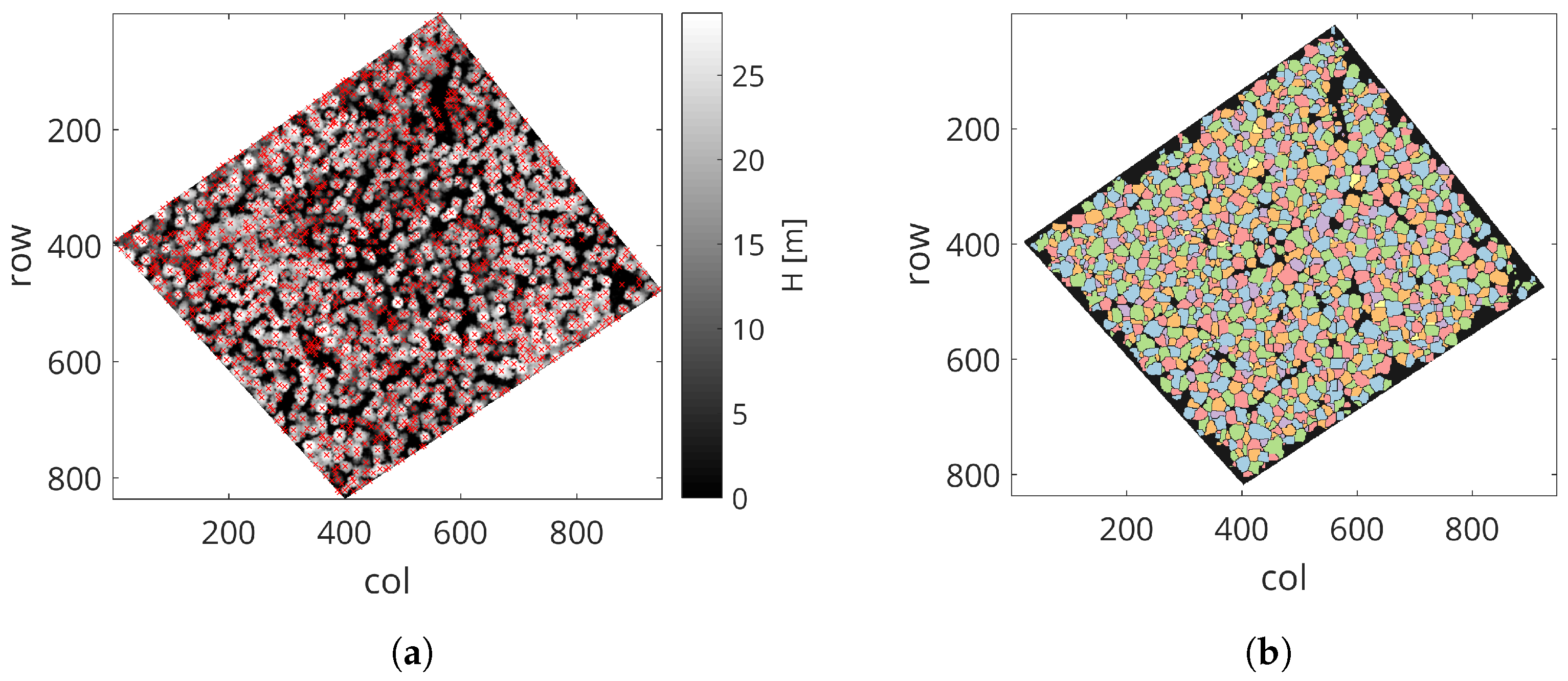
Figure 3.
(a) Tree top detection results with variable size convolution window. (b) Raster CHM segmentation obtained with the marker controlled watershed algorithm.
Figure 3.
(a) Tree top detection results with variable size convolution window. (b) Raster CHM segmentation obtained with the marker controlled watershed algorithm.

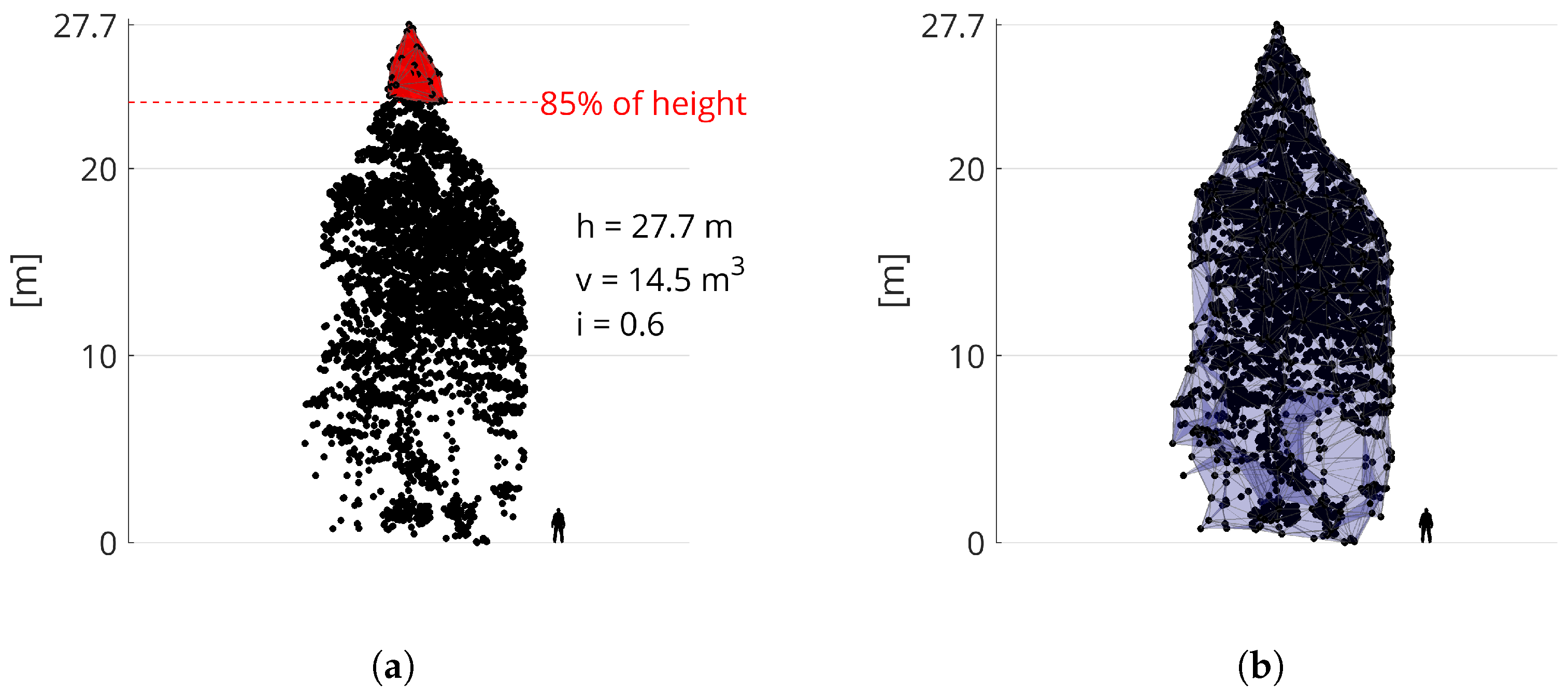
Figure 4.
(a) The total height (h), the 3D convex alpha shape (in red) volume (v) and the median intensity (i) of points located in the top 15 % of the tree crown are used as features because they are less affected by poor segmentation. (b) The single region 3D alpha shape (outlined in blue) derived from the point cloud segment.

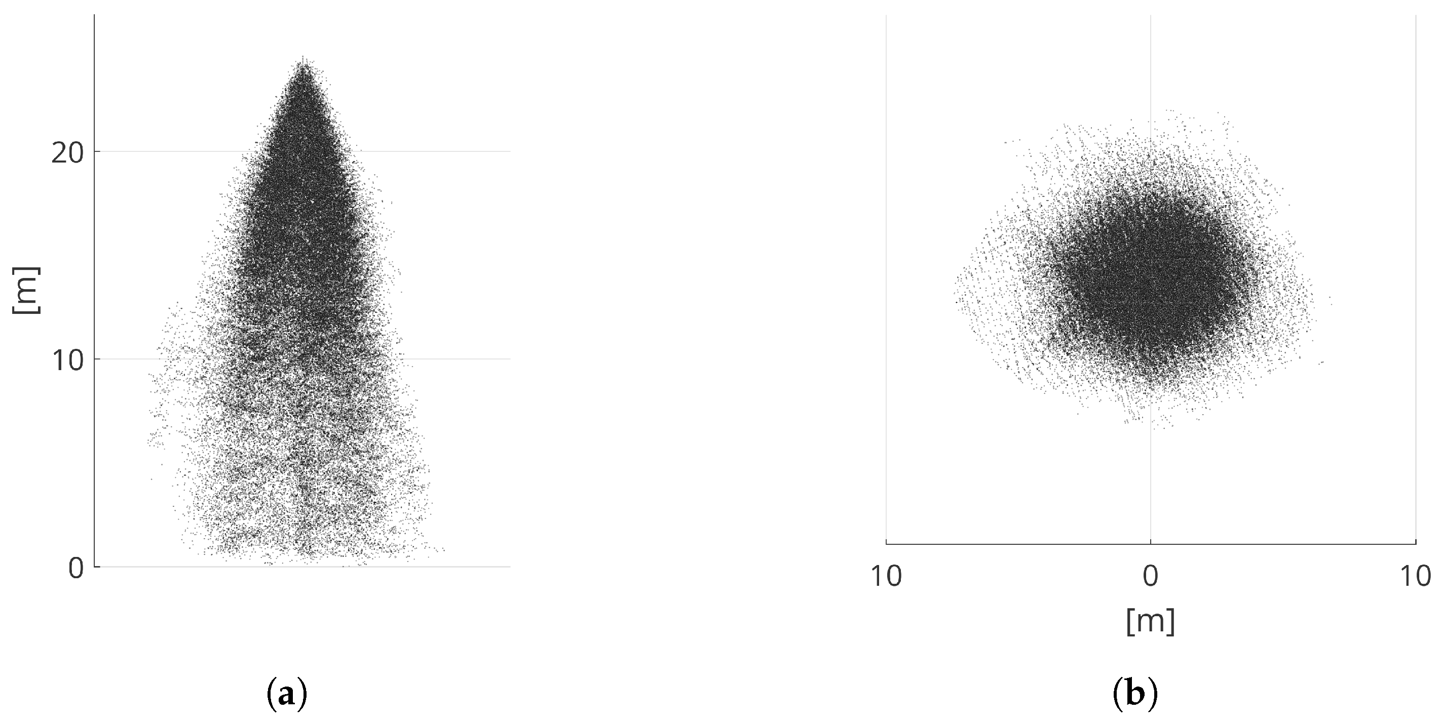
Figure 5.
Example of an ensemble containing 69 overlaid segments with similar features. Dense point areas indicate high shape probability. (a) Side view (b) Top view.
Figure 5.
Example of an ensemble containing 69 overlaid segments with similar features. Dense point areas indicate high shape probability. (a) Side view (b) Top view.

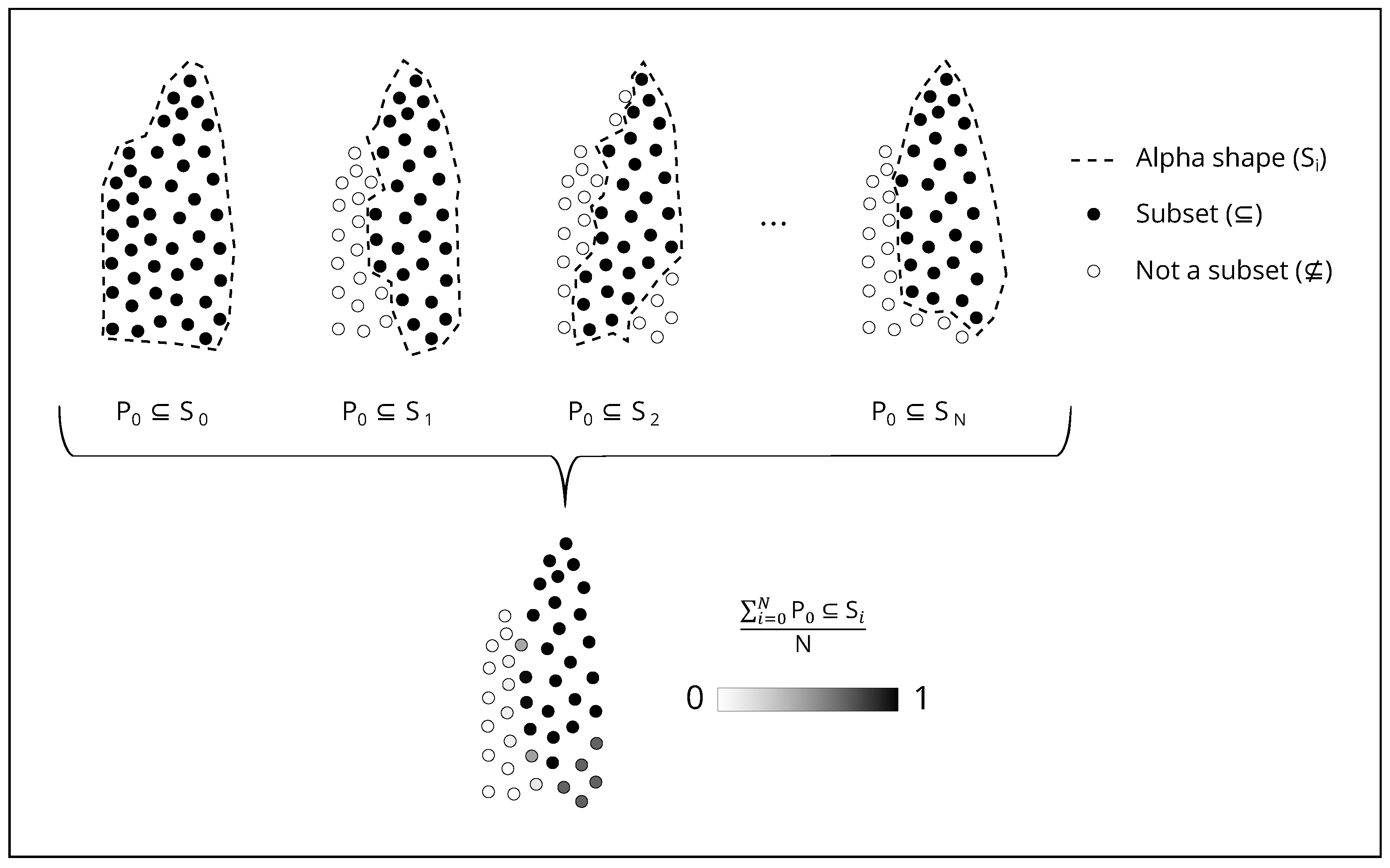
Figure 6.
Each point cloud segment is overlaid with the alpha shapes of similar segments (including itself). Regions of the point cloud segment which occur more frequently inside obtain a higher shape probability. Thus, inconsistencies between the shapes in the ensemble can be detected.
Figure 6.
Each point cloud segment is overlaid with the alpha shapes of similar segments (including itself). Regions of the point cloud segment which occur more frequently inside obtain a higher shape probability. Thus, inconsistencies between the shapes in the ensemble can be detected.

Figure 7.
Individual segment delineation accuracy. The reference shape (in gray) represents the extent of the manually delineated tree. For visualization purposes, the boundaries of the union (in orange) and intersection (in blue) alpha shapes are spatially separated from the points. In reality, the alpha shape boundary passes though the boundary points.

Figure 8.
Sensitivity of the median validation scores to . Notice that the delineation scores are undefined when the detection rate reaches 0.
Figure 8.
Sensitivity of the median validation scores to . Notice that the delineation scores are undefined when the detection rate reaches 0.

Figure 9.
Boxplots of delineation scores before and after filtering the segments with . All the delineation scores except recall are significantly higher after filtering. It can also be noted that the filtering reduces the score spread.
Figure 9.
Boxplots of delineation scores before and after filtering the segments with . All the delineation scores except recall are significantly higher after filtering. It can also be noted that the filtering reduces the score spread.

Figure 10.
(a) Shape probability map (high vegetation only). (b) Side (first row) and top (second row) view of shape probability for six example segments. Notice that segment n°3 has null probability. This is explained by the fact it is a particularly high tree and there was an insufficient number of similar trees to form a reliable ensemble. (c) Filtered segments using .


Table 1.
Study site metadata. These attributes refer to the central 1.97 ha area indicated by the yellow polygon in Figure 1b.
Table 1.
Study site metadata. These attributes refer to the central 1.97 ha area indicated by the yellow polygon in Figure 1b.
| Topography | Aspect | East-northeast |
| Slope | ~10° | |
| Forest Plot | Density (DBH ≥ 12.5 cm) | 382 per ha |
| Basal area per ha | 28.4 m2/ha | |
| Composition (by count) | Abies alba (38%), Picea abies (33%), Fagus sylvatica (28%), Acer Pseudoplatanus (1%) | |
| Canopy layering | Mostly single layered |
Table 2.
Airborne Laser Scanning (ALS) acquisition metadata. The measurement configuration refers only to the three sites used in this study (not the complete ALS acquisition). The echo digitization, intensity normalization and point cloud classification were done by the data provider.
Table 2.
Airborne Laser Scanning (ALS) acquisition metadata. The measurement configuration refers only to the three sites used in this study (not the complete ALS acquisition). The echo digitization, intensity normalization and point cloud classification were done by the data provider.
| Platform and Instrumentation | Aircraft | Cessna T206H |
| LiDAR scanner | Riegl LMS-Q1560 | |
| Camera | Phase One iXA 180-R50 | |
| GNSS-Inertial System | Applanix POS/AV 610 Trimble AP60 with IMU57 | |
| Measurement Configuration | Acquisition dates | 4–5 May 2016 |
| Phenology | leaf-off | |
| Sensor to surface range (mean ± std) | 675 ± 38 m | |
| Pulse repetition rate | 800 kHz | |
| Aircraft speed | 176 km/h | |
| Min/max scan angle | ± 30° | |
| Median point density (in forest areas) | 30 m−2 | |
| Post-Processing | Echo digitization | Riegl RiProcess |
| Ground filtering | Progressive TIN densification (TerraScan implementation) |
Table 3.
Criteria used to create ensembles (groups) of similar segments.
| Feature | Criteria |
|---|---|
| Total height | |
| Upper crown convex hull volume | |
| Upper crown median intensity |
Table 4.
Comparison of detection and median delineation performance (before|after) filtering the segments with . Scores were rounded to the nearest second decimal. : number of observations, d: detection rate, p: precision, r: recall, F: F-score, : pointwise intersection over union, : volumewise intersection over union, : areawise intersection over union.
| Height [m] | Obs. | Detection d | Delineation | |||||
|---|---|---|---|---|---|---|---|---|
| p | r | F | ||||||
| 118 | 0.58 0.49 | 0.65 0.92 | 0.96 0.83 | 0.74 0.84 | 0.58 0.73 | 0.47 0.65 | 0.58 0.73 | |
| 182 | 0.57 0.51 | 0.60 0.93 | 0.94 0.81 | 0.71 0.81 | 0.55 0.69 | 0.48 0.64 | 0.53 0.71 | |
| 454 | 0.59 0.51 | 0.68 0.95 | 0.96 0.84 | 0.75 0.87 | 0.60 0.76 | 0.51 0.69 | 0.56 0.77 | |
| Overall | 754 | 0.58 0.51 | 0.65 0.94 | 0.96 0.83 | 0.74 0.85 | 0.58 0.74 | 0.49 0.67 | 0.56 0.75 |
© 2018 by the authors. Licensee MDPI, Basel, Switzerland. This article is an open access article distributed under the terms and conditions of the Creative Commons Attribution (CC BY) license (http://creativecommons.org/licenses/by/4.0/).
Share and Cite
MDPI and ACS Style
Parkan, M.; Tuia, D. Estimating Uncertainty of Point-Cloud Based Single-Tree Segmentation with Ensemble Based Filtering. Remote Sens. 2018, 10, 335. https://doi.org/10.3390/rs10020335
AMA Style
Parkan M, Tuia D. Estimating Uncertainty of Point-Cloud Based Single-Tree Segmentation with Ensemble Based Filtering. Remote Sensing. 2018; 10(2):335. https://doi.org/10.3390/rs10020335
Chicago/Turabian StyleParkan, Matthew, and Devis Tuia. 2018. "Estimating Uncertainty of Point-Cloud Based Single-Tree Segmentation with Ensemble Based Filtering" Remote Sensing 10, no. 2: 335. https://doi.org/10.3390/rs10020335
Note that from the first issue of 2016, this journal uses article numbers instead of page numbers. See further details here.