Atmospheric Correction Inter-Comparison Exercise

 , , , and
Abstract
:
1. Introduction
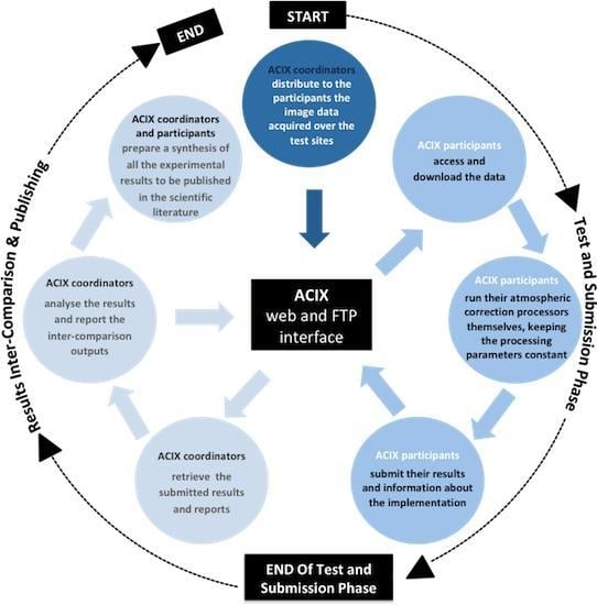
2. ACIX Protocol
2.1. ACIX Sites and Datasets
Input Data and Processing Specifications
2.2. Inter-Comparison Analysis
2.2.1. Aerosol Optical Thickness (AOT) and Water Vapour (WV)
2.2.2. Surface Reflectance (SR)
Inter-Comparison of the Retrieved SRs
Comparison with AERONET Corrected Data
3. Overview of ACIX Results
3.1. Landsat-8
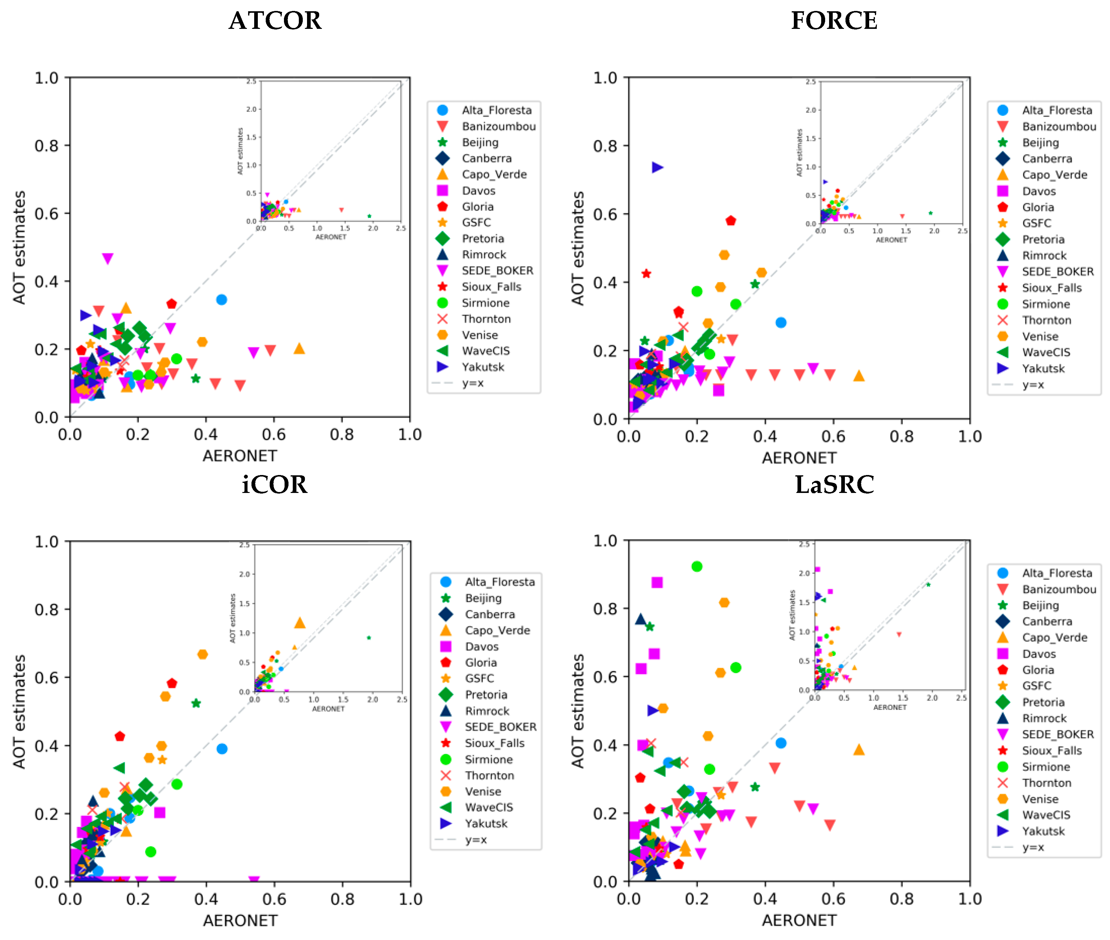
3.1.1. Aerosol Optical Thickness
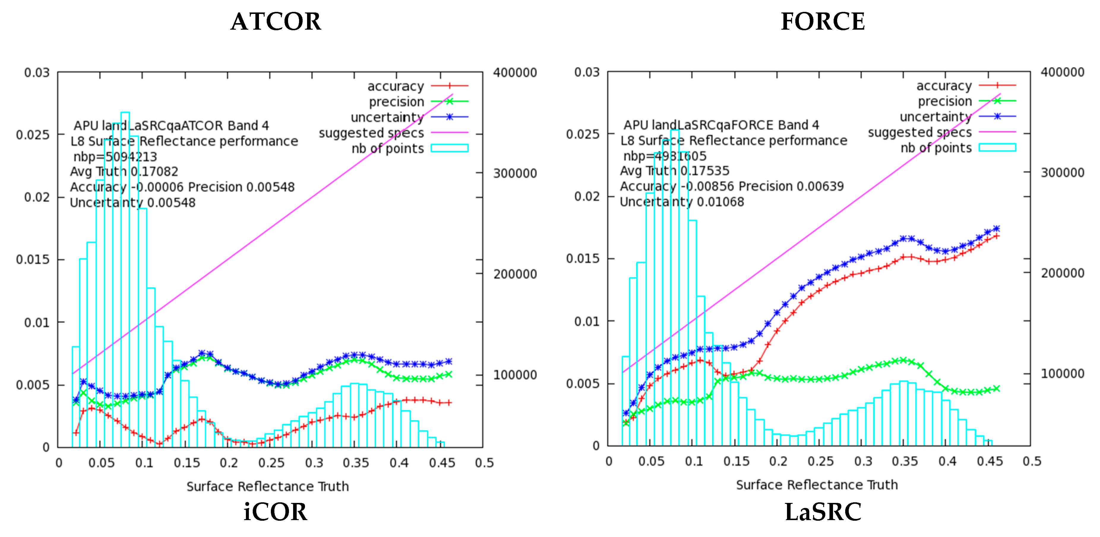
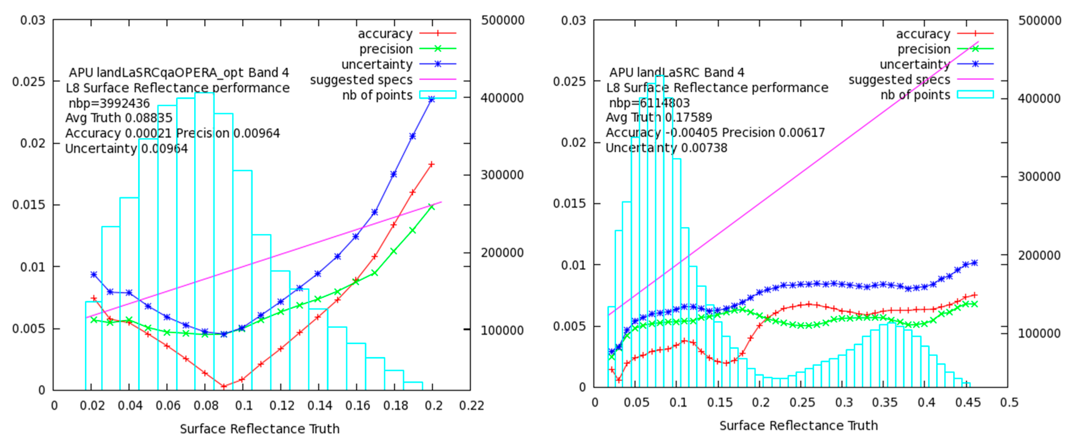
3.1.2. Surface Reflectance Products
3.2. Sentinel-2
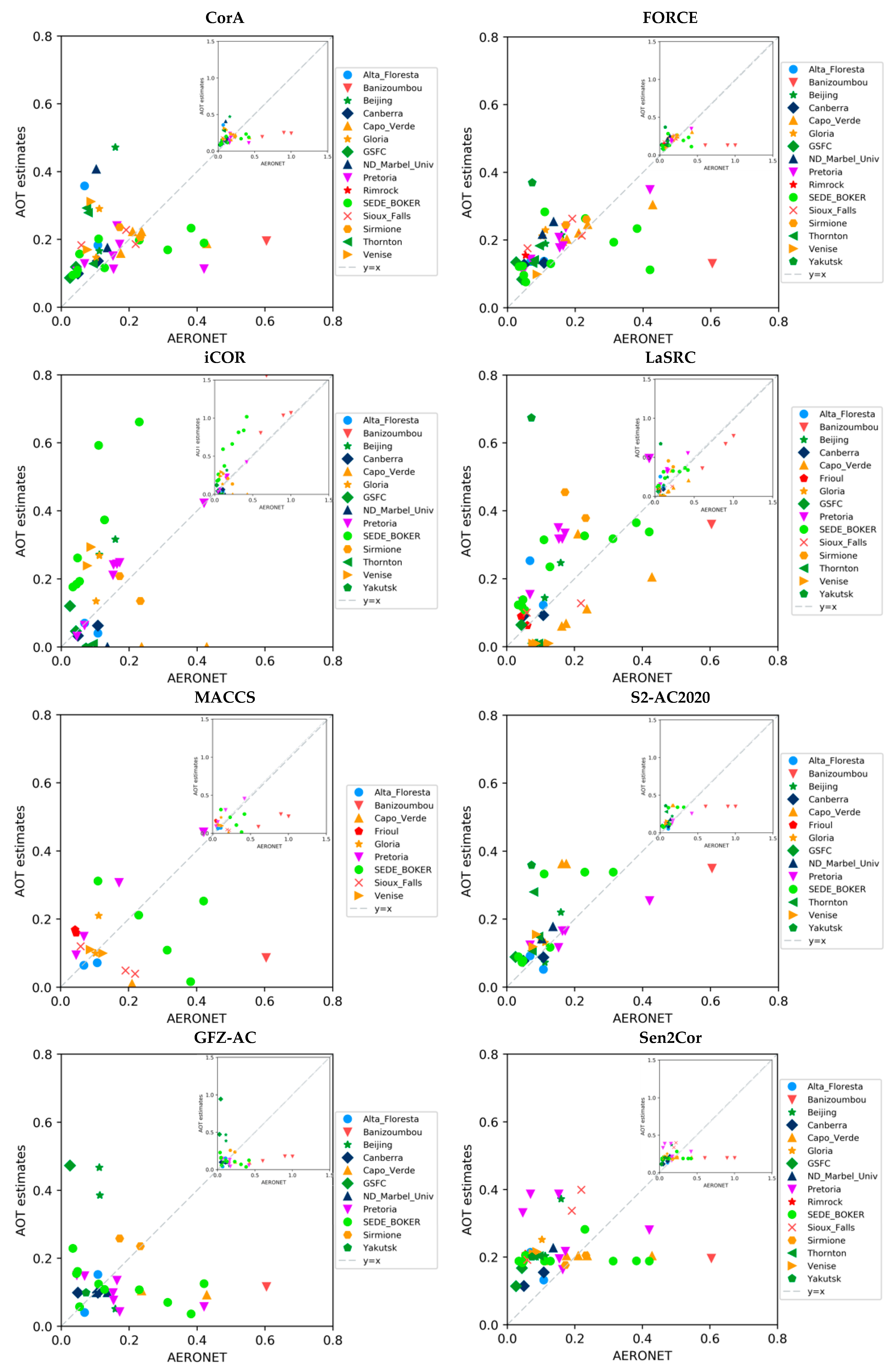
3.2.1. Aerosol Optical Thickness
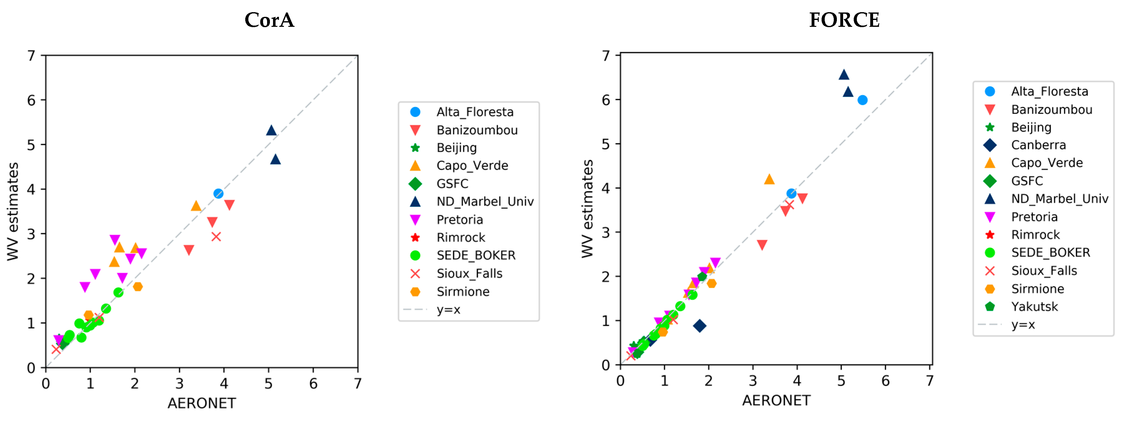
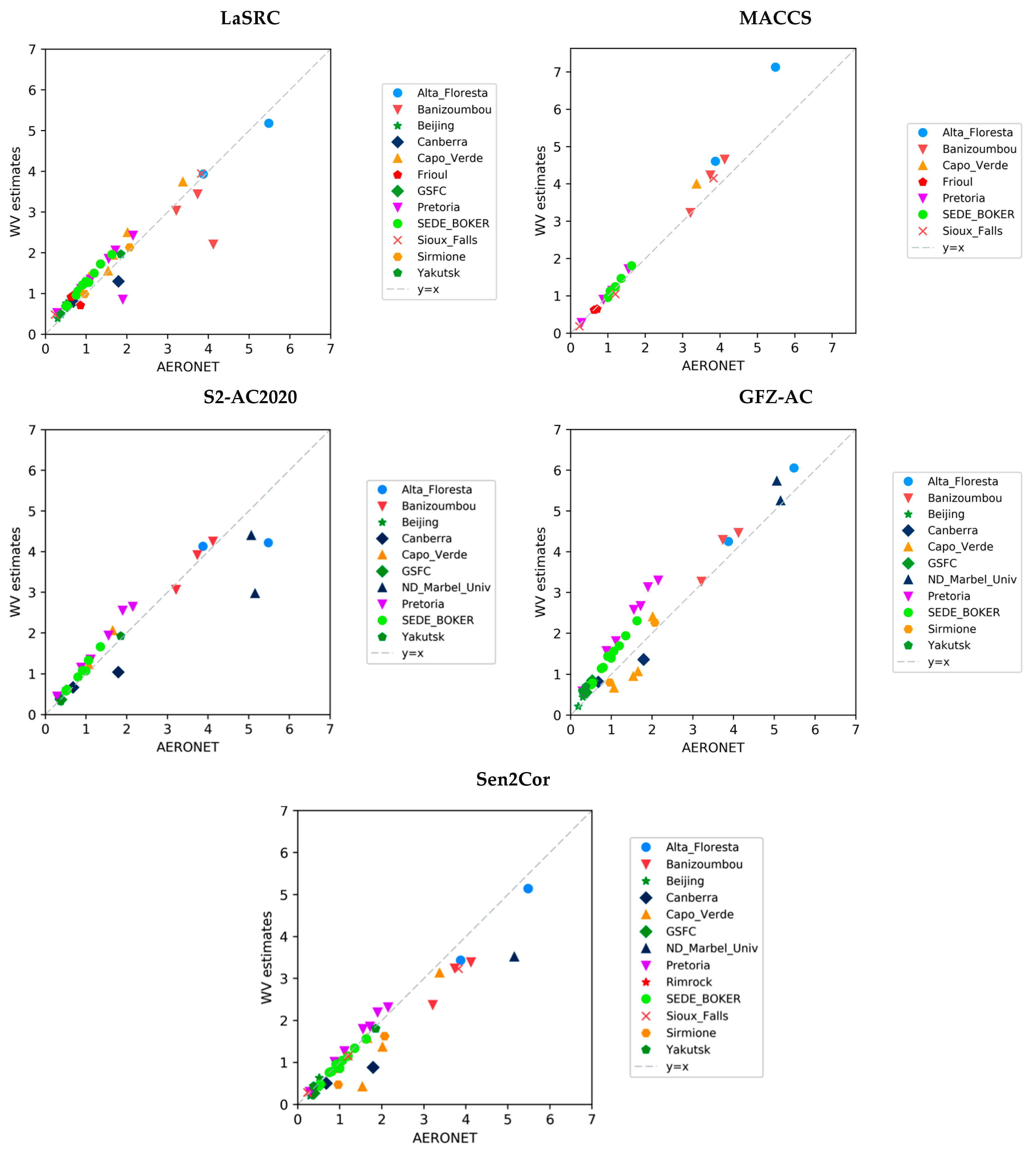
3.2.2. Water Vapour (WV)
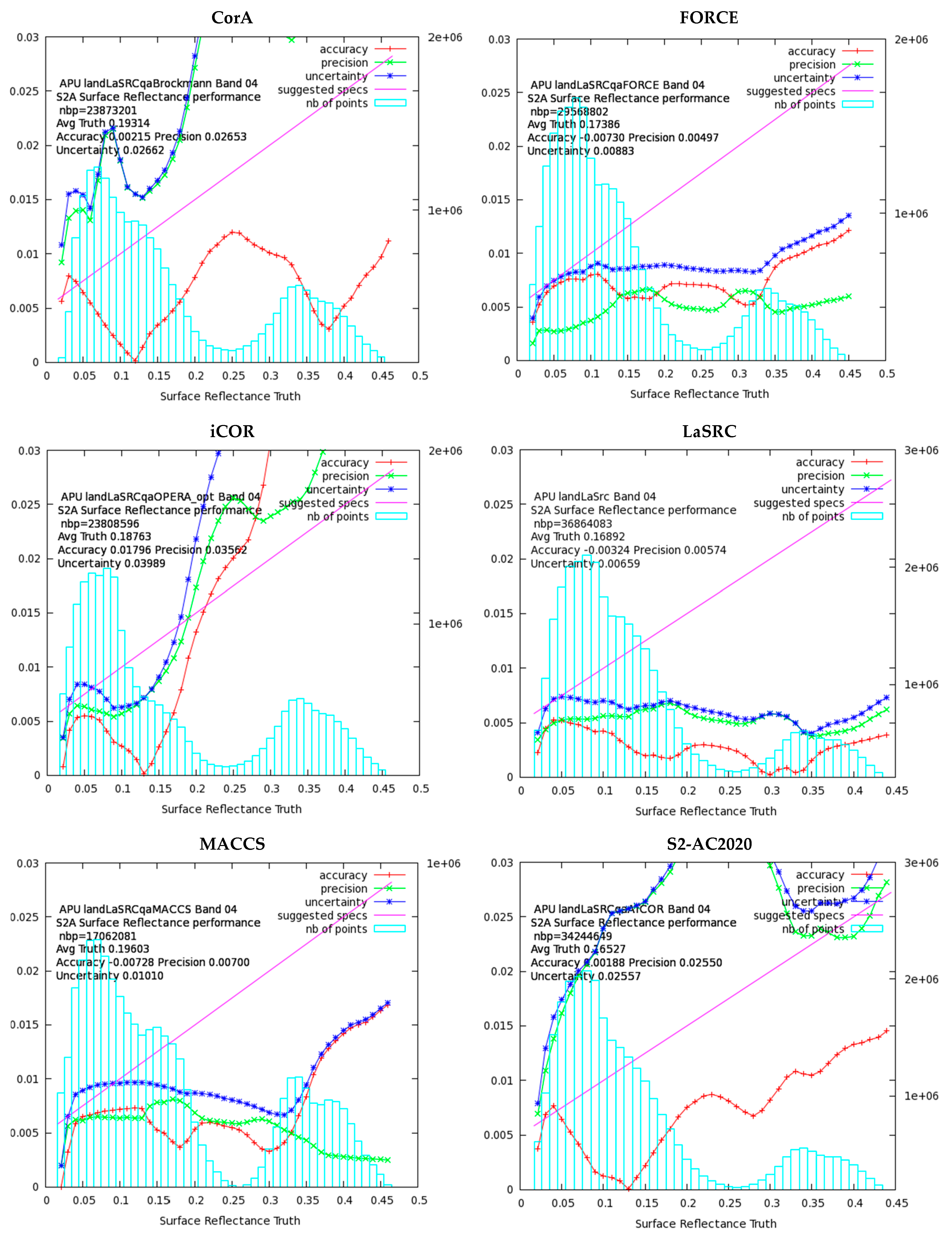
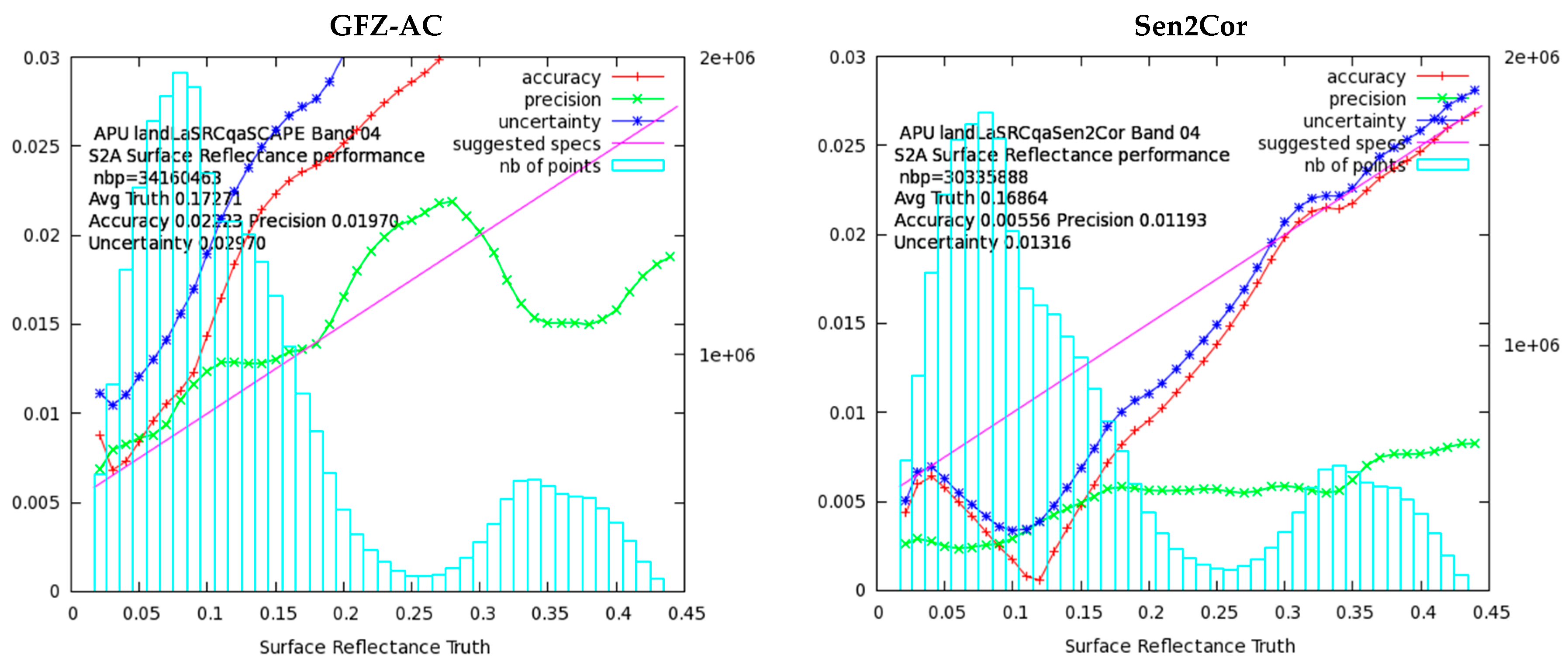
3.2.3. Surface Reflectance Products
4. Conclusions
Acknowledgments
Author Contributions
Conflicts of Interest
References
- Vermote, E.F.; Kotchenova, S. Atmospheric correction for the monitoring of land surfaces. J. Geophys. Res. 2008, 113. [Google Scholar] [CrossRef]
- Franch, B.; Vermote, E.F.; Roger, J.C.; Murphy, E.; Becker-Reshef, I.; Justice, C.; Claverie, M.; Nagol, J.; Csiszar, I.; Meyer, D.; et al. A 30+ Year AVHRR Land Surface Reflectance Climate Data Record and Its Application to Wheat Yield Monitoring. Remote Sens. 2017, 9, 296. [Google Scholar] [CrossRef]
- Hagolle, O.; Huc, M.; Villa Pascual, D.; Dedieu, G. A multi-temporal and multi-spectral method to estimate aerosol optical thickness over land, for the atmospheric correction of FormoSat-2, LandSat, VENµS and Sentinel-2 images. Remote Sens. 2015, 7, 2668–2691. [Google Scholar] [CrossRef]
- Ng, W.T.; Rima, P.; Einzmann, K.; Immitzer, M.; Atzberger, C.; Eckert, S. Assessing the Potential of Sentinel-2 and Pléiades Data for the Detection of Prosopis and Vachellia spp. in Kenya. Remote Sens. 2017, 9, 74. [Google Scholar] [CrossRef]
- Van der Werff, H.; Van der Meer, F. Sentinel-2A MSI and Landsat 8 OLI Provide Data Continuity for Geological Remote Sensing. Remote Sens. 2016, 8, 883. [Google Scholar] [CrossRef]
- Radoux, J.; Chomé, G.; Jacques, D.C.; Waldner, F.; Bellemans, N.; Matton, N.; Lamarche, C.; d’Andrimont, R.; Defourny, P. Sentinel-2’s Potential for Sub-Pixel Landscape Feature Detection. Remote Sens. 2016, 8, 488. [Google Scholar] [CrossRef]
- Pahlevan, N.; Sarkar, S.; Franz, B.A.; Balasubramanian, S.V.; He, J. Sentinel-2 MultiSpectral Instrument (MSI) data processing for aquatic science applications: Demonstrations and validations. Remote Sens. Environ. 2017, 201, 47–56. [Google Scholar] [CrossRef]
- Pahlevan, N.; Schott, J.R.; Franz, B.A.; Zibordi, G.; Markham, B.; Bailey, S.; Schaaf, C.B.; Ondrusek, M.; Greb, S.; Strait, C.M. Landsat 8 remote sensing reflectance (R rs) products: Evaluations, intercomparisons, and enhancements. Remote Sens. Environ. 2017, 190, 289–301. [Google Scholar] [CrossRef]
- Rouquié, B.; Hagolle, O.; Bréon, F.-M.; Boucher, O.; Desjardins, C.; Rémy, S. Using Copernicus Atmosphere Monitoring Service Products to Constrain the Aerosol Type in the Atmospheric Correction Processor MAJA. Remote Sens. 2017, 9, 1230. [Google Scholar] [CrossRef]
- Dörnhöfer, K.; Göritz, A.; Gege, P.; Pflug, B.; Oppelt, N. Water Constituents and Water Depth Retrieval from Sentinel-2A—A First Evaluation in an Oligotrophic Lake. Remote Sens. 2016, 8, 941. [Google Scholar] [CrossRef]
- Ju, J.; Roy, D.P.; Vermote, E.; Masek, J.; Kovalskyy, V. Continental-scale validation of MODIS-based and LEDAPS Landsat ETM+ atmospheric correction methods. Remote Sens. Environ. 2012, 122, 175–184. [Google Scholar] [CrossRef]
- Claverie, M.; Vermote, E.F.; Franch, B.; Masek, J.G. Evaluation of the Landsat-5 TM and Landsat-7 ETM+ surface reflectance products. Remote Sens. Environ. 2015, 169, 390–403. [Google Scholar] [CrossRef]
- Vermote, E.; Justice, C.; Claverie, M.; Franch, B. Preliminary analysis of the performance of the Landsat 8/OLI land surface reflectance product. Remote Sens. Environ. 2016, 185, 46–56. [Google Scholar] [CrossRef]
- Holben, B.N.; Eck, T.F.; Slutsker, I.; Tanre, D.; Buis, J.P.; Setzer, A.; Vermote, E.; Reagan, J.A.; Kaufman, Y.J.; Nakajima, T.; et al. AERONET—A federated instrument network and data archive for aerosol characterization. Remote Sens. Environ. 1998, 66, 1–16. [Google Scholar] [CrossRef]
- Smirnov, A.; Holben, B.N.; Eck, T.F.; Dubovik, O.; Slutsker, I. Cloud-screening and quality control algorithms for the AERONET database. Remote Sens. Environ. 2000, 73, 337–349. [Google Scholar] [CrossRef]
- Richter, R. Correction of satellite imagery over mountainous terrain. Appl. Opt. 1998, 37, 4004–4015. [Google Scholar] [CrossRef] [PubMed]
- Richter, R.; Schläpfer, D. Atmospheric/Topographic Correction for Satellite Imagery; DLR Report DLR-IB 565-02/15); German Aerospace Center (DLR): Wessling, Germany, 2015. [Google Scholar]
- Defourny, P.; Arino, O.; Boettcher, M.; Brockmann, C.; Kirches, G.; Lamarche, C.; Radoux, J.; Ramoino, F.; Santoro, M.; Wevers, J. CCI-LC ATBDv3 Phase II. Land Cover Climate Change Initiative—Algorithm Theoretical Basis Document v3. Issue 1.1, 2017. Available online: https://www.esa-landcover-cci.org/?q=documents# (accessed on 20 February 2018).
- Frantz, D.; Röder, A.; Stellmes, M.; Hill, J. An Operational Radiometric Landsat Preprocessing Framework for Large-Area Time Series Applications. IEEE Trans. Geosci. Remote Sens. 2016, 54, 3928–3943. [Google Scholar] [CrossRef]
- Li, F.; Jupp, D.L.B.; Thankappan, M.; Lymburner, L.; Mueller, N.; Lewis, A.; Held, A. A Physics-based Atmospheric and BRDF Correction for Landsat Data over Mountainous Terrain. Remote Sens. Environ. 2012, 124, 756–770. [Google Scholar] [CrossRef]
- Franz, B.A.; Bailey, S.W.; Kuring, N.; Werdell, P.J. Ocean color measurements with the Operational Land Imager on Landsat-8: Implementation and evaluation in SeaDAS. J. Appl. Remote Sens. 2015, 9, 096070. [Google Scholar] [CrossRef]
- Vermote, E.F.; Tanré, D.; Deuze, J.L.; Herman, M.; Morcette, J.J. Second simulation of the satellite signal in the solar spectrum, 6S: An overview. IEEE Trans. Geosci. Remote Sens. 1997, 35, 675–686. [Google Scholar] [CrossRef]
- Dubovik, O.; Holben, B.; Eck, T.F.; Smirnov, A.; Kaufman, Y.J.; King, M.D.; Tanré, D.; Slutsker, I. Variability of absorption and optical properties of key aerosol types observed in worldwide locations. J. Atmos. Sci. 2002, 59, 590–608. [Google Scholar] [CrossRef]
- Kotchenova, S.Y.; Vermote, E.F.; Matarrese, R.; Klemm, F.J. Validation of a vector version of the 6S radiative transfer code for atmospheric correction of satellite data. Part I: Path radiance. Appl. Opt. 2006, 45, 6762–6774. [Google Scholar] [CrossRef] [PubMed]
- Kotchenova, S.Y.; Vermote, E.F. Validation of a vector version of the 6S radiative transfer code for atmospheric correction of satellite data. Part II. Homogeneous Lambertian and anisotropic surfaces. Appl. Opt. 2007, 46, 4455–4464. [Google Scholar] [CrossRef] [PubMed]
- Petrucci, B.; Huc, M.; Feuvrier, T.; Ruffel, C.; Hagolle, O.; Lonjou, V.; Desjardins, C. MACCS: Multi-Mission Atmospheric Correction and Cloud Screening tool for high-frequency revisit data processing. In Proceedings of the Image and Signal Processing for Remote Sensing XXI, Toulouse, France, 21–24 September 2015. [Google Scholar]


| AC Processor | Participants | Affiliation | Reference | Data Submitted | |
|---|---|---|---|---|---|
| Landsat-8 | Sentinel-2 | ||||
| ACOLITE | Quinten Vanhellmont | Royal Belgian Institute for Natural Sciences [Belgium] | - | ✓ | ✓ |
| ATCOR/S2-AC2020 | Bringfried Pflug, Rolf Richter, Aliaksei Makarau | DLR German Aerospace Center [Germany] | [16,17] | ✓ | ✓ |
| CorA [Brockmann] | Grit Kirches, Carsten Brockmann | Brockmann Consult GmbH [Germany] | [18] | - | ✓ |
| FORCE | David Frantz, Joachim Hill | Trier University [Germany] | [19] | ✓ | ✓ |
| iCOR [OPERA] | Stefan Adriaensen | VITO [Belgium] | - | ✓ | ✓ |
| GA-PABT | Fuqin Li | Geoscience Australia [Australia] | [20] | ✓ | ✓ |
| LAC | Antoine Mangin | ACRI [France] | - | - | ✓ |
| LaSRC | Eric Vermote | GSFC NASA [USA] | [13] | ✓ | ✓ |
| MACCS | Olivier Hagolle | CNES [France] | [3] | - | ✓ |
| GFZ-AC [SCAPE-M] | André Hollstein | GFZ German Research Centre for Geosciences [Germany] | - | - | ✓ |
| SeaDAS | Nima Pahlevan | GSFC NASA [USA] | [7,8,21] | ✓ | - |
| Sen2Cor v2.2.2 | Jerome Louis | Telespazio France [France] | - | - | ✓ |
| Bringfried Pflug | DLR German Aerospace Center [Germany] | ||||
| Test Sites * | Zone ** | Land Cover | Aeronet Station | |
|---|---|---|---|---|
| Lat., Lon. | ||||
| Temperate | Carpentras [France] | Temperate | vegetated, bare soil, coastal | 44.083, 5.058 |
| Davos [Switzerland] | Temperate | forest, snow, agriculture | 46.813, 9.844 | |
| Beijing [China] | Temperate | urban, mountains | 39.977, 116.381 | |
| Canberra [Australia] | Temperate | urban, vegetated, water | −35.271, 149.111 | |
| Pretoria_CSIR-DPSS [South Africa] | Temperate | urban, semi-arid | −25.757, 28.280 | |
| Sioux_Falls [USA] | Temperate | cropland, vegetated | 43.736, −96.626 | |
| GSFC [USA] | Temperate | urban, forest, cropland, water | 38.992, −76.840 | |
| Yakutsk [Russia] | Temperate | forest, river, snow | 61.662, 129.367 | |
| Arid | Banizoumbou [Niger] | Tropical | desert, cropland | 13.541, 2.665 |
| Capo_Verde [Capo Verde] | Tropical | desert, ocean | 16.733, −22.935 | |
| SEDE_BOKER [Israel] | Temperate | desert | 34.782, 30.855 | |
| Equatorial Forest | Alta_Floresta [Brazil] | Tropical | cropland, urban, forest | −9.871, −56.104 |
| ND_Marbel_Univ [Philippines] | Tropical | cropland, urban, forest | 6.496, 124.843 | |
| Boreal | Rimrock [USA] | Temperate | semi-arid | 46.487, −116.992 |
| Coastal | Thornton C-power [Belgium] | Temperate | water, vegetated | 51.532, 2.955 |
| Gloria [Romania] | Temperate | water, vegetated | 44.600, 29.360 | |
| Sirmione_Museo_GC [Italy] | Temperate | water, vegetated, urban | 45.500, 10.606 | |
| Venice [Italy] | Temperate | water, vegetated, urban | 45.314, 12.508 | |
| WaveCIS_Site_CSI_6 [USA] | Temperate | water, vegetated | 28.867, −90.483 |
| AC Processor 1 | AC Processor 2 | AC Processor 3 | … | AC Processor n | |
|---|---|---|---|---|---|
| AC Processor 1 | 0 | d12 | d13 | … | d1n |
| AC Processor 2 | d21 | 0 | d23 | … | d2n |
| AC Processor 3 | d31 | d32 | 0 | … | d3n |
| …. | … | … | … | … | … |
| AC Processor n | dn1 | dn2 | dn3 | … | 0 |
| AC Processor-Reference AOT | |||||
|---|---|---|---|---|---|
| No. of Samples | Min | Mean | ±RMS (stdv) | Max | |
| ATCOR | 120 | 0 | 0.122 | 0.207 | 1.844 |
| FORCE | 124 | 0.002 | 0.112 | 0.211 | 1.745 |
| iCOR | 111 | 0.002 | 0.095 | 0.119 | 1.015 |
| LaSRC | 119 | 0.001 | 0.233 | 0.387 | 2.017 |
| OLI Band | ATCOR | FORCE | LaSRC | iCOR | |
|---|---|---|---|---|---|
| nbp | 5094039 | 4981438 | 6109550 | 3985227 | |
| 1 | A | 0.009 | 0.009 | −0.005 | −0.004 |
| P | 0.010 | 0.008 | 0.010 | 0.011 | |
| U | 0.013 | 0.012 | 0.012 | 0.012 | |
| 2 | A | 0.001 | −0.001 | −0.004 | −0.004 |
| P | 0.007 | 0.006 | 0.009 | 0.010 | |
| U | 0.007 | 0.006 | 0.010 | 0.010 | |
| 3 | A | 0.000 | −0.009 | −0.004 | 0.000 |
| P | 0.005 | 0.006 | 0.007 | 0.009 | |
| U | 0.005 | 0.010 | 0.008 | 0.009 | |
| 4 | A | 0.000 | −0.009 | −0.004 | 0.000 |
| P | 0.005 | 0.006 | 0.006 | 0.010 | |
| U | 0.005 | 0.011 | 0.007 | 0.010 | |
| 5 | A | 0.005 | 0.000 | −0.005 | 0.010 |
| P | 0.005 | 0.005 | 0.007 | 0.010 | |
| U | 0.008 | 0.005 | 0.008 | 0.014 | |
| 6 | A | −0.001 | −0.023 | −0.002 | 0.006 |
| P | 0.004 | 0.012 | 0.003 | 0.006 | |
| U | 0.004 | 0.026 | 0.004 | 0.008 | |
| 7 | A | −0.001 | −0.008 | 0.001 | 0.006 |
| P | 0.006 | 0.007 | 0.003 | 0.005 | |
| U | 0.006 | 0.010 | 0.003 | 0.007 |
| AC Processor-Reference AOT | |||||
|---|---|---|---|---|---|
| No. of Samples | Min | Mean | ±RMS (Stdv) | Max | |
| CorA | 47 | 0 | 0.133 | 0.155 | 0.757 |
| FORCE | 48 | 0.003 | 0.116 | 0.169 | 0.871 |
| iCOR | 37 | 0.002 | 0.15 | 0.151 | 0.599 |
| LaSRC | 48 | 0.002 | 0.115 | 0.097 | 0.602 |
| MACCS | 24 | 0.002 | 0.176 | 0.2 | 0.778 |
| S2-AC2020 | 36 | 0.002 | 0.107 | 0.144 | 0.652 |
| GFZ-AC | 41 | 0.001 | 0.159 | 0.223 | 0.92 |
| Sen2Cor | 47 | 0.005 | 0.158 | 0.147 | 0.805 |
| AC Processor-Reference WV | |||||
|---|---|---|---|---|---|
| No. of Samples | Min | Mean | ±RMS (Stdv) | Max | |
| CorA | 36 | 0.008 | 0.37 | 0.332 | 1.312 |
| FORCE | 43 | 0.001 | 0.215 | 0.305 | 1.504 |
| LaSRC | 41 | 0.021 | 0.297 | 0.303 | 1.906 |
| MACCS | 20 | 0.002 | 0.269 | 0.387 | 1.654 |
| S2-AC2020 | 29 | 0.005 | 0.344 | 0.437 | 2.18 |
| GFZ-AC | 39 | 0.027 | 0.457 | 0.283 | 1.246 |
| Sen2Cor | 41 | 0.012 | 0.28 | 0.346 | 1.63 |
| MSI Band | CorA | FORCE | iCOR | LaSRC | MACCS | S2-AC2020 | GFZ-AC | Sen2Cor | |
|---|---|---|---|---|---|---|---|---|---|
| nbp | 23873202 | 29568870 | 23808647 | 36863274 | 12538144 | 34243490 | 34159390 | 30335882 | |
| 1 | A | −0.006 | −0.002 | −0.010 | −0.010 | - | −0.006 | 0.026 | −0.003 |
| P | 0.096 | 0.009 | 0.024 | 0.010 | - | 0.017 | 0.014 | 0.011 | |
| U | 0.096 | 0.009 | 0.026 | 0.014 | - | 0.018 | 0.029 | 0.011 | |
| 2 | A | 0.000 | −0.004 | 0.000 | −0.007 | −0.008 | −0.004 | 0.023 | −0.001 |
| P | 0.021 | 0.007 | 0.028 | 0.008 | 0.010 | 0.021 | 0.016 | 0.009 | |
| U | 0.021 | 0.008 | 0.028 | 0.011 | 0.013 | 0.022 | 0.029 | 0.009 | |
| 3 | A | 0.003 | −0.012 | 0.013 | −0.005 | −0.008 | 0.000 | 0.031 | 0.004 |
| P | 0.024 | 0.006 | 0.034 | 0.006 | 0.008 | 0.023 | 0.023 | 0.010 | |
| U | 0.025 | 0.014 | 0.036 | 0.008 | 0.012 | 0.023 | 0.039 | 0.011 | |
| 4 | A | 0.002 | −0.007 | 0.018 | −0.003 | −0.007 | 0.002 | 0.022 | 0.006 |
| P | 0.027 | 0.005 | 0.036 | 0.006 | 0.007 | 0.025 | 0.020 | 0.012 | |
| U | 0.027 | 0.009 | 0.040 | 0.007 | 0.010 | 0.026 | 0.030 | 0.013 | |
| 5 | A | 0.008 | −0.008 | 0.027 | −0.002 | −0.005 | 0.007 | 0.031 | 0.020 |
| P | 0.029 | 0.005 | 0.038 | 0.006 | 0.006 | 0.012 | 0.022 | 0.018 | |
| U | 0.030 | 0.009 | 0.046 | 0.006 | 0.008 | 0.014 | 0.038 | 0.027 | |
| 6 | A | 0.005 | 0.001 | 0.024 | −0.001 | −0.003 | 0.004 | 0.024 | 0.017 |
| P | 0.032 | 0.005 | 0.033 | 0.005 | 0.006 | 0.010 | 0.042 | 0.011 | |
| U | 0.032 | 0.005 | 0.041 | 0.005 | 0.007 | 0.011 | 0.049 | 0.021 | |
| 7 | A | 0.006 | −0.002 | 0.025 | −0.003 | −0.007 | 0.005 | 0.020 | 0.014 |
| P | 0.033 | 0.005 | 0.031 | 0.005 | 0.005 | 0.009 | 0.047 | 0.010 | |
| U | 0.034 | 0.006 | 0.040 | 0.005 | 0.008 | 0.010 | 0.051 | 0.017 | |
| 8 | A | 0.008 | 0.017 | 0.032 | 0.001 | −0.001 | 0.011 | 0.025 | 0.022 |
| P | 0.033 | 0.010 | 0.034 | 0.005 | 0.005 | 0.026 | 0.047 | 0.014 | |
| U | 0.034 | 0.019 | 0.047 | 0.005 | 0.006 | 0.028 | 0.053 | 0.026 | |
| 8a | A | −0.008 | 0.000 | 0.023 | −0.002 | −0.008 | 0.003 | 0.016 | 0.013 |
| P | 0.033 | 0.005 | 0.028 | 0.004 | 0.005 | 0.011 | 0.049 | 0.008 | |
| U | 0.034 | 0.005 | 0.036 | 0.005 | 0.009 | 0.011 | 0.051 | 0.015 | |
| 11 | A | 0.021 | −0.010 | 0.018 | 0.002 | −0.003 | 0.009 | 0.017 | 0.020 |
| P | 0.035 | 0.005 | 0.019 | 0.003 | 0.003 | 0.007 | 0.011 | 0.009 | |
| U | 0.041 | 0.011 | 0.026 | 0.003 | 0.004 | 0.011 | 0.020 | 0.022 | |
| 12 | A | 0.020 | 0.004 | 0.013 | 0.004 | 0.000 | 0.008 | 0.014 | 0.025 |
| P | 0.030 | 0.006 | 0.013 | 0.003 | 0.002 | 0.006 | 0.019 | 0.014 | |
| U | 0.036 | 0.007 | 0.018 | 0.005 | 0.003 | 0.010 | 0.024 | 0.028 |
© 2018 by the authors. Licensee MDPI, Basel, Switzerland. This article is an open access article distributed under the terms and conditions of the Creative Commons Attribution (CC BY) license (http://creativecommons.org/licenses/by/4.0/).
Share and Cite
Doxani, G.; Vermote, E.; Roger, J.-C.; Gascon, F.; Adriaensen, S.; Frantz, D.; Hagolle, O.; Hollstein, A.; Kirches, G.; Li, F.; et al. Atmospheric Correction Inter-Comparison Exercise. Remote Sens. 2018, 10, 352. https://doi.org/10.3390/rs10020352
Doxani G, Vermote E, Roger J-C, Gascon F, Adriaensen S, Frantz D, Hagolle O, Hollstein A, Kirches G, Li F, et al. Atmospheric Correction Inter-Comparison Exercise. Remote Sensing. 2018; 10(2):352. https://doi.org/10.3390/rs10020352
Chicago/Turabian StyleDoxani, Georgia, Eric Vermote, Jean-Claude Roger, Ferran Gascon, Stefan Adriaensen, David Frantz, Olivier Hagolle, André Hollstein, Grit Kirches, Fuqin Li, and et al. 2018. "Atmospheric Correction Inter-Comparison Exercise" Remote Sensing 10, no. 2: 352. https://doi.org/10.3390/rs10020352