Land Cover Classification Using Integrated Spectral, Temporal, and Spatial Features Derived from Remotely Sensed Images


1
College of Water Conservancy and Civil Engineering, Inner Mongolia Agricultural University, Hohhot 010018, China
2
Insitute of Remote Sensing and Digital Earth (RADI), Chinese Academy of Sciences, Beijing 100101, China
3
College of Forestry, Inner Mongolia Agricultural University, Hohhot 010018, China
*
Author to whom correspondence should be addressed.
Remote Sens. 2018, 10(3), 383; https://doi.org/10.3390/rs10030383
Submission received: 28 January 2018
/
Revised: 25 February 2018
/
Accepted: 27 February 2018
/
Published: 1 March 2018
(This article belongs to the Special Issue Classification and Feature Extraction for Remote Sensing Image Analysis)
Abstract
:Obtaining accurate and timely land cover information is an important topic in many remote sensing applications. Using satellite image time series data should achieve high-accuracy land cover classification. However, most satellite image time-series classification methods do not fully exploit the available data for mining the effective features to identify different land cover types. Therefore, a classification method that can take full advantage of the rich information provided by time-series data to improve the accuracy of land cover classification is needed. In this paper, a novel method for time-series land cover classification using spectral, temporal, and spatial information at an annual scale was introduced. Based on all the available data from time-series remote sensing images, a refined nonlinear dimensionality reduction method was used to extract the spectral and temporal features, and a modified graph segmentation method was used to extract the spatial features. The proposed classification method was applied in three study areas with land cover complexity, including Illinois, South Dakota, and Texas. All the Landsat time series data in 2014 were used, and different study areas have different amounts of invalid data. A series of comparative experiments were conducted on the annual time-series images using training data generated from Cropland Data Layer. The results demonstrated higher overall and per-class classification accuracies and kappa index values using the proposed spectral-temporal-spatial method compared to spectral-temporal classification methods. We also discuss the implications of this study and possibilities for future applications and developments of the method.
1. Introduction
Mapping land cover distribution and monitoring its dynamics have been identified as an important goal in environmental studies [1,2,3,4,5]. Land cover maps provide fundamental information for many applications, including global change analysis, crop yield estimation, and forest management [6,7,8]. Land cover maps can be easily generated using remote sensing images, but ensuring their accuracy is much more difficult [9]. To improve the accuracy of classification, most land cover products use multi-temporal images as their inputs [10,11,12,13,14]. Currently, the primary method of land cover classification using multi-temporal data involves obtaining metrics from time series (i.e., the phenological characteristics of different vegetation), and the slope, elevation, maximum, minimum, mean, standard deviation values and tasseled cap transformation of spectral-temporal features and spectral indices [15,16,17,18,19,20,21]. Then the metrics are classified in a supervised approach. While these metrics have verified that the spectral-temporal features defining the various land cover classes are well captured, the use of the multi-temporal images introduces other issues that must be solved.
To date, most classification methods require input images with few clouds. However, this standard cannot be met by sensors with low temporal frequency, such as the Landsat series of satellites. Global land images derived from the Enhanced Thematic Mapper Plus have about 35% cloud coverage on average [22], indicating that cloud cover is common in optical remote sensing images. The presence of cloud cover increases the difficulty of image analysis and limits the utility of optical remote sensing images. Two solutions are commonly used for cloud removal in multi-temporal images. One method is to replace the cloudy temporal data with data from images without clouds or snow taken in the same season but different years. As a result, most land cover products are mapped at intervals of 5 or 10 years, which significantly reduces “currency” [23,24,25]. The other method entails filling cloudy locations using per-pixel temporal compositing procedures via adjacent temporal interpolation, a time-series curve filter or inversion of n-day observations to estimate reflectance based on the bidirectional reflectance distribution function [26,27,28,29]. These methods do not increase information content, but may introduce gross errors, particularly when continuous temporal data are unavailable. It is worth noting that, because of the low temporal frequency of the Landsat satellite, the data obtained are rarely completely cloudless and most images contain cloud cover. When cloud coverage reaches a threshold such as 30%, the temporal image is deemed unusable and the remaining 70% of the image will also be discarded [30]. In other words, for a given satellite time series, the temporal dimension of each pixel may be not the same, despite using the same period. Therefore, only methods that work with unequal time series will be able to fully exploit the available data.
Using multi-spectral time-series data also causes data redundancy problems, because there is a high correlation between time-series images of unchanged regions [31,32,33]. This point has been widely adopted in the research of change detection using remotely-sensed data [34,35,36,37,38]. Therefore, it is necessary to reduce the dimension of multi-spectral time series prior to land cover classification, particularly for methods that use full-band satellite image time series as input [15,39,40]. Dimensionality reduction (DR) techniques project high-dimension data into a low-dimensional space to maximize valuable information while minimizing noise [41,42]. Numerous DR approaches for processing remote sensing hyperspectral images have been proposed [43,44,45,46], which can be broadly divided into two types: linear and nonlinear methods. Due to multiple scattering effects off different ground components, the reflectance in remote sensing images is not linearly proportional to surface area. Multi-spectral and time-series data have intrinsic nonlinear characteristics [39]. However, little research has been devoted to the application of nonlinear DR techniques to multi-spectral remote sensing time series.
At present, most of multi-temporal land cover classification methods are based on spectral-temporal information without consideration of dependencies between adjacent pixels. As we all known, spatial information is very helpful for the improvement of classification accuracy [47,48,49,50,51]. Spectral-spatial classification of hyperspectral images shows improvements in classification accuracy compared to only spectral-based methods [47,48,49,50,51]. Therefore, how to combine spatial information in time series land cover classification is a problem worthy of studying. Image segmentation is the main method employed to obtain spatial information [52,53]. There are a lot of algorithms for image segmentation. However, this method cannot be directly applied to multi-spectral time-series images because temporal information cannot be used in this context [54]. Therefore, it is urgent to have a method to preform segmentation based on spectral-temporal information for multi-spectral time series images.
In this paper, we investigated the potential for extracting spectral-temporal and spatial features from satellite time-series data to reliably classify different land cover categories. Our focus is on an automatic and stable classification approach without human intervention to improve the accuracy and reduce the mapping period for land cover products. In addition, the temporal dimension is completely integrated into modeling. Our overall research objectives were to solve the high dimensionality problem of multi-spectral time series using all the available data, and to determine how to extract and combine the spatial characteristics of time-series land cover classifications. To achieve these objectives, we developed a new automated time-series land cover classification method based on extracting spectral-temporal and spatial features using all the available data. This methodology is applicable to all of satellite time series but is illustrated using Landsat time series data in this study. Specifically, the dynamic time warping (DTW) similarity measure was used on satellite image time series to mine all the available data. Then, a modification of a nonlinear DR method developed for hyperspectral data was used to extract spectral-temporal features from multi-spectral satellite time series, and an image segmentation method was modified to extract spatial features from multi-spectral satellite time series. Finally, a classification system based on spatial regularization is established to generate land cover map using spectral-temporal and spatial features.
2. Study Area and Data
2.1. Study Area
Our study focused on agricultural states including Illinois, South Dakota, and Texas, which cover the latitudinal range of the United States. Due to climatic differences among different regions, the main land cover classes in these three areas differed. Major crop types from the South Dakota study area in the northern United States include soybeans, corn, and alfalfa. Major crop types from the Illinois study area in the central United States include soybeans, corn, and pasture and grassland. The main crop types from the Texas study area in the southern United States include corn, cotton, pasture and grassland, and winter wheat. Since the major crop types used in this study were planted once a year, such as corn and soybeans, we assume that land cover classes will not change within 1 year in the study areas.
2.2. Data
2.2.1. Satellite Data
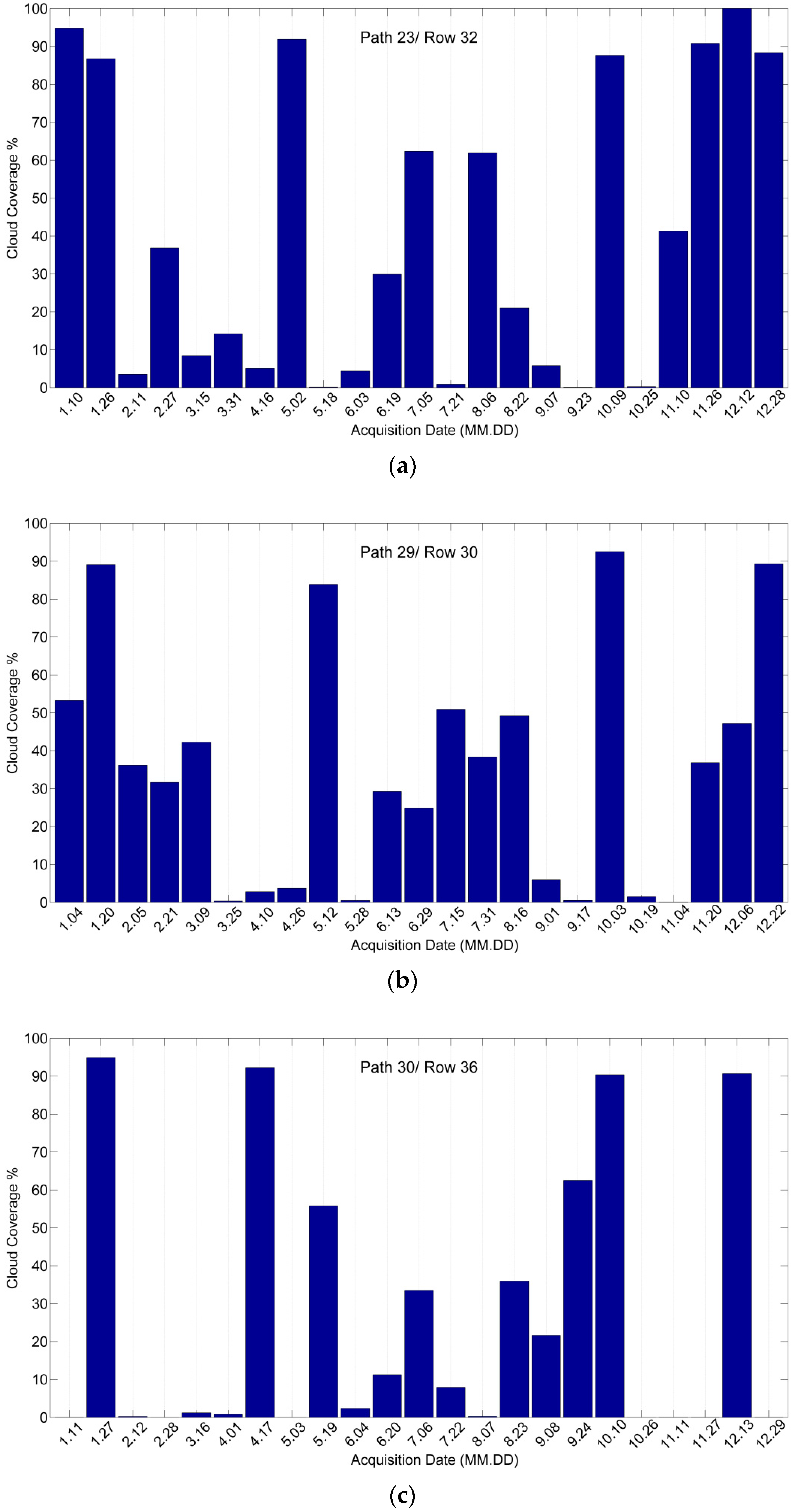
Landsat 8 Operational Land Imager (OLI) data were obtained from the Unites States Geological Survey web site (http://earthexplorer.usgs.gov/). The repeat cycle of Landsat 8 is 16 days, and thus each WRS-2 path/row can be obtained up to 22 or 23 scenes per year [55,56,57]. In this study, all the 23 images acquired by Landsat 8 OLI L1T in 2014 of the study areas were used. We used the Landsat OLI reflective bands with 30 m spatial resolution, which included bands 1 (coastal), 2 (blue), 3 (green), 4 (red), 5 (near-infrared), 6 (middle-infrared), and 7 (middle-infrared), along with two cloud masks. Band 9 (cirrus) was not used because it is sensitive to water absorption [58]. Three study areas were comprised of 100,000, 125,000 and 160,000 30 m pixels were cut from the Landsat 8 OLI Path 23/Row 32, Path 29/Row 30 and Path 30/Row 36 images, respectively. Figure 1a–c show the acquisition date and cloud coverage of each scene. The corresponding reference data were extracted from the Cropland Data Layer (CDL). Due to the computation of the Laplacian Eigenmaps (LE) DR algorithm increases rapidly with spatial dimension, larger regions were not used in this study.
2.2.2. Reference Data
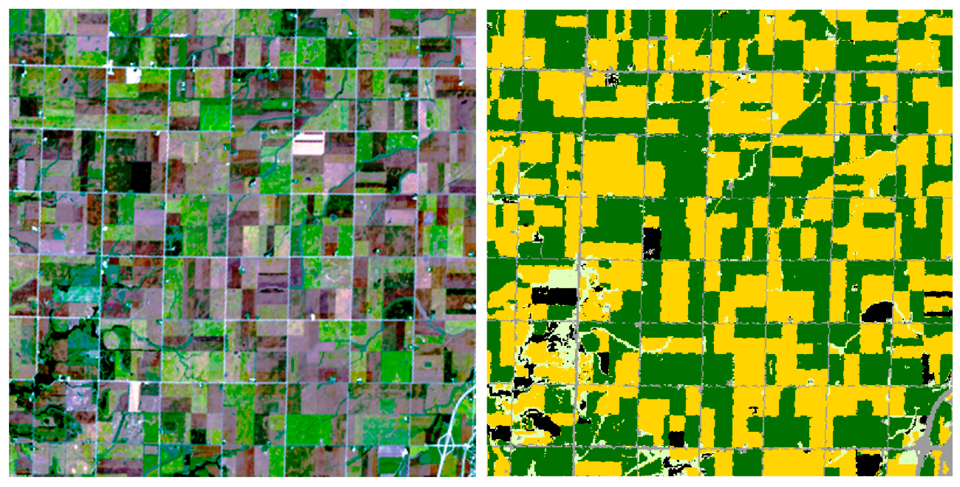
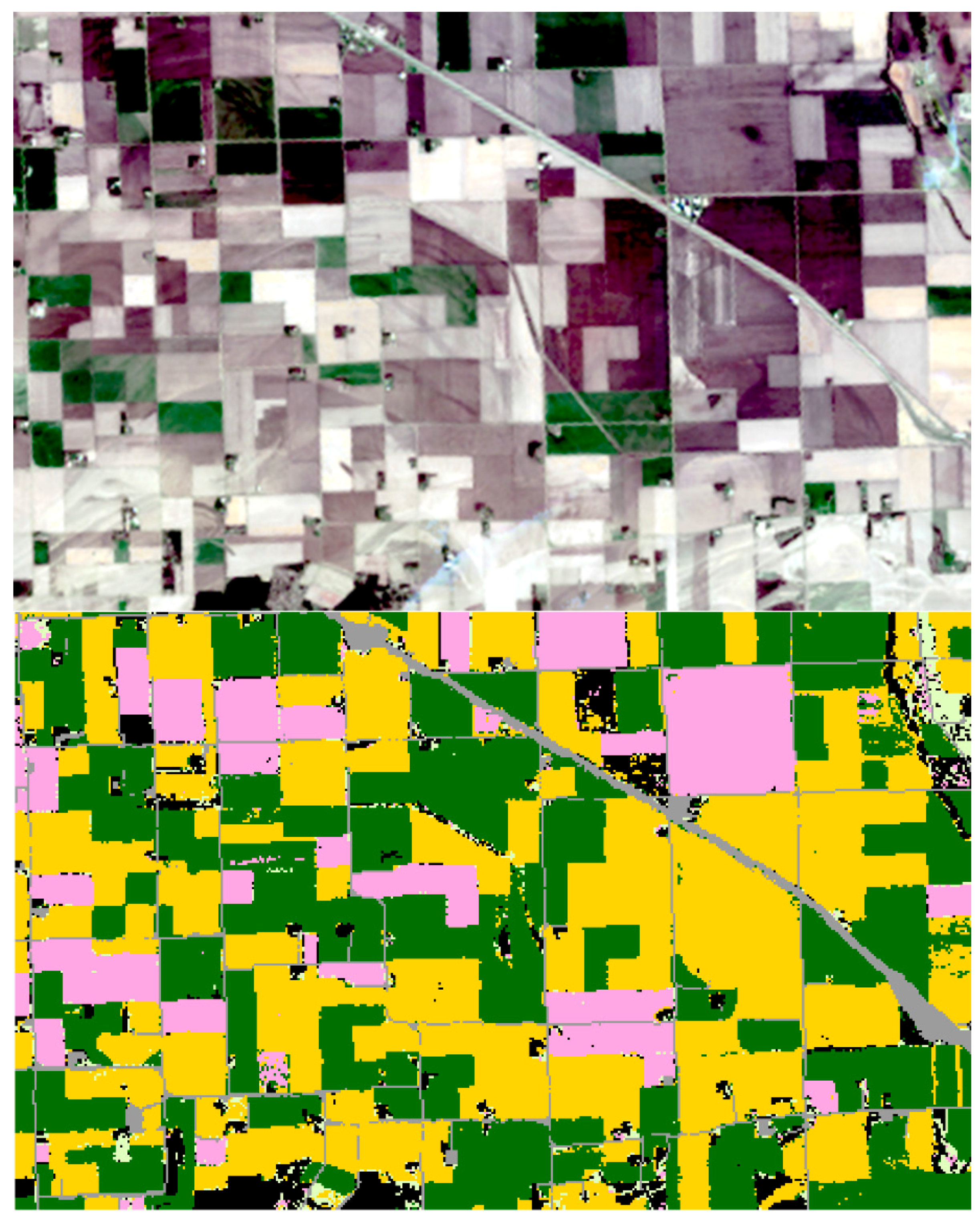
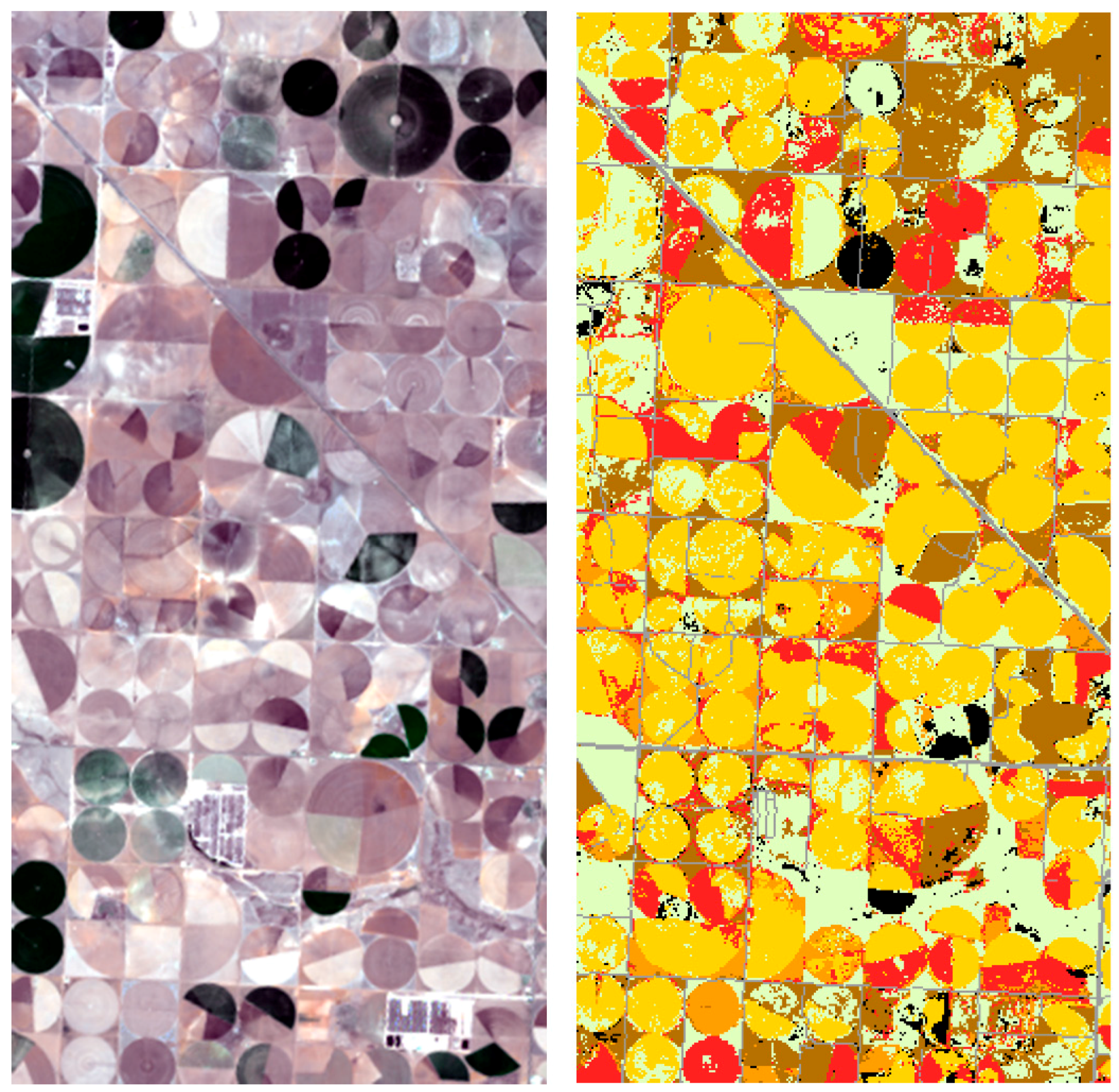
The CDL for 2014 provided by the United States Department of Agriculture (USDA) National Agricultural Statistics Service (NASS) was obtained from the CDL web site (http://nassgeodata.gmu.edu/CropScape/) [59]. The CDL is a raster-formatted, georeferenced, crop-specific, land cover map. The CDL was widely used as a training and testing data source for supervised land cover classification [12]. The CDL is generated annually by a decision tree-supervised non-parametric classification method using moderate spatial resolution satellite imagery and ground-truth observations collected by the USDA. In total, 110 land cover classes were defined in the CDL product with a 30 m spatial resolution [60]. Figure 2, Figure 3 and Figure 4 illustrate the reference data (2014 CDL data) for the three study areas with the standard color legends used by the USDA NASS. The percentage of each class in each study area according to the CDL data is also listed in the titles of figures.
3. Data Processing and Methodology
3.1. Image Preprocessing
In this study, only Landsat L1T images were used. The raw DN values are converted into surface reflectance using atmospheric correction tool from the Landsat Ecosystem Disturbance Adaptive Processing System [61]. To effectively use the characteristics of the spectral variation, we arranged all the temporal data for each band together to build a time series. Each image had a corresponding cloud mask file defining the geographic areas that were affected by cloud cover. Values were removed from the time series if the cloud mask file indicated they were affected by clouds. As a result, the number of pixels varied among time series. We often encounter images with cloud cover in remote sensing time-series data. Fully exploiting the available observations requires a method that can be used with unequal time series. In addition, many phenomena of interest, such as vegetation phenology, exhibit periodic behavior that can be affected by weather variation. These adjustments result in the extension or compression of the temporal profiles. This phenomenon indicates that observed ground objects may exhibit irregular temporal behavior. Therefore, methods that are stable to temporal distortions are needed.
The DTW similarity measure [62,63] makes it possible to use all of the available data to analyze the temporal features of remote sensing time series. DTW uses the optimal alignment of radiometric profiles to describe the similarity between two temporal profiles with shifted or distorted evolution and irregular sampling. When there are invalid data in a remote sensing time series, the ideal solution is to remove only the invalid data, while preserving all the valid data. This solution requires a similarity measure that can compare time series with unequal lengths (representing different temporal sampling intervals). In contrast to classic similarity measures used to compare time series, DTW is not restricted to the comparison of time series with equal lengths. DTW can realign time series to assess nonlinear distortions on the temporal axis [64]. Therefore, DTW cannot only compare time series with unequal lengths, but can find the optimal warping path for the two time series [65].
The methodology of DTW is as follows. Assume a time series T of length n, and a time series S of length m.
The time series T and S can be ordered to form an n-by-m path matrix where every element of matrix (i, j), corresponds to a queue between the points and . The warping path is subject to the following constraints [63]:
Endpoint constraint: the warping path must start from the first point (,) of the path matrix and end at the last point (,) of the path matrix.
Continuity constraint: the steps in the path matrix are confined to neighboring points, and .
Monotonicity: the path must advance monotonically with respect to time, and .
DTW is used to calculate the cumulative distance to each point based on the following dynamic programming formulation:
where denotes the distance measure between and , for example, the square of the difference or the magnitude of the difference.
In the search space determined by two time series, the cumulative distance of the warping path found by DTW is minimum among all possible paths. Figure 5 shows the path matrix and optimal warping path (indicated by red squares) between time series T and S using DTW.
3.2. Time Series Dimensionality Reduction
In this study, the LE DR algorithm is refined. The reasons for choosing the LE DR algorithm are as follows. First, LE is a nonlinear manifold learning method, which has been proven to perform better than linear DR methods when applied to hyperspectral data [43,66,67,68,69]. Second, LE is a local manifold learning (LML) method. The advantage of LML method is that the local attributes of the original data can be preserved by constructing a neighborhood graph when projected from high-dimensionality to low-dimensionality space. Using a neighborhood graph implicitly emphasizes the natural clusters in the data, in contrast to global methods, for example, ISOMAP [70]. Third, LE is a graph-based method, which only requires similarity between data points to complete DR, thereby making it easy to combine different distance metrics compared to other localization-preserving methods [71,72,73,74,75].
In this study, an improved version of LE called LE-DTW was proposed. In the LE-DTW DR method, DTW is used instead of Euclidean distance to find the k nearest neighbors for each sample in the original feature space. If specific dimensions in the feature space for some pixels are invalid (e.g., covered by cloud or snow), these values will be removed during the construction of sequences (Section 3.1) before DR. Therefore, all the available data are used in the process of building an adjacency graph using DTW. For example, given a dataset and , where n denotes the number of data points and t denotes the dimensionality of the data, the adjacency graph W can be constructed with an edge between nodes i and j if and are the nearest neighbors of each other. If nodes i and j are connected, then
where the parameter q is a predetermined constant; otherwise, set . Let D represent a diagonal matrix and set . Now the matrix L = D − W is the so-called Laplacian matrix, it is symmetrical and positive semi-definite. Next, solve the generalized eigenvector problem
Let be S + 1 eigenvectors corresponding to eigenvalues . Because the smallest eigenvalue , we discard and use the next S eigenvectors for embedding in S-dimensional Euclidian space using the map
There are two parameters that need to be manually set in the LE DR method. One is the number of nearest neighbors selected for each pixel, abbreviated k. Another is the number of bands retained after DR. In this study, the parameter k is automatically determined in the LE-DTW DR method using a “graph growing” strategy [76]. This strategy increases the probability that any pixel and its neighbors belong to the same ground object and selects a different number of nearest neighbors for each pixel. The 10 DR bands corresponding to the 10 smallest non-zero eigenvalues were selected for classification. The number of DR bands is greater than the maximum number of classes in the image (six classes in the Texas study area) to ensure that adequate information was retained in the DR bands [39]. A reasonable minimum number of bands after DR cannot be determined using the existing approaches. Because these existing approaches cannot handle unequal time series [77,78]. For simplicity, all the DR methods employed in this study reduced the data to 10 dimensions.
3.3. Time Series Spatial Feature Extraction
To perform image segmentation is the main approach to obtain spatial information for classification. Segmentation is a comprehensive partitioning of the input image into objects, each of which consists of a set of pixels that are homogeneous with respect to some criterion [79]. These objects form a segmentation map that provides spatial structures and features for object-oriented classification [80] or post-classification optimization [47]. In many segmentation methods, the image elements are mapped onto a graph. Then, the problem of segmenting an image becomes the problem of partitioning a graph. No discretization is the advantage of graph segmentation because it has completely combinatorial operator, and therefore it does not accumulate discretization errors [81].
The minimum spanning tree (MST) is a classic method in graph theory [82]. The graph vertices are connected to satisfy the minimum cumulative edge weights, and partitioning of the graph is performed by removing the edges to obtain non-overlapping sub-graphs. The criterion of segmentation methods based on MST is to remove the edges with the greatest weights. The edge weights are determined by a similarity measure between pixels [83]. Two commonly used methods of computing the MST are Kruskal’s algorithm [84] and Prim’s algorithm [85]. In this study, we presented a method called MST-DTW for automatic segmentation of multi-spectral time-series imagery. This method sets the edges and their weights based on the DTW measure using all the valid data in the time series to build a graph. It is worth noting that each edge on a graph can only connect the center node and its eight nearest neighbors in a 3 × 3 window. We chose Prim’s algorithm, which constructs the MST by iteratively adding the frontier edge with the smallest weight. Given a multi-spectral time series, we constructed the input data using the segmentation method described in Section 3.1. Assuming Q × R total pixels in the input data, the eight-connection graph is defined as follows. Assume that the set of all vertices in is
where the are the image pixels. Then the set of all edges in is denoted by
where are the edges that connect node and one of its eight adjacent nodes . For each edge , we set a weight that is the result of DTW measurement between two node vectors
Then the weighted graph is
where W is the set of w values corresponding to the weight of each edge .
Then, according to the undirected graph , we constructed an MST using the tree spanning given by
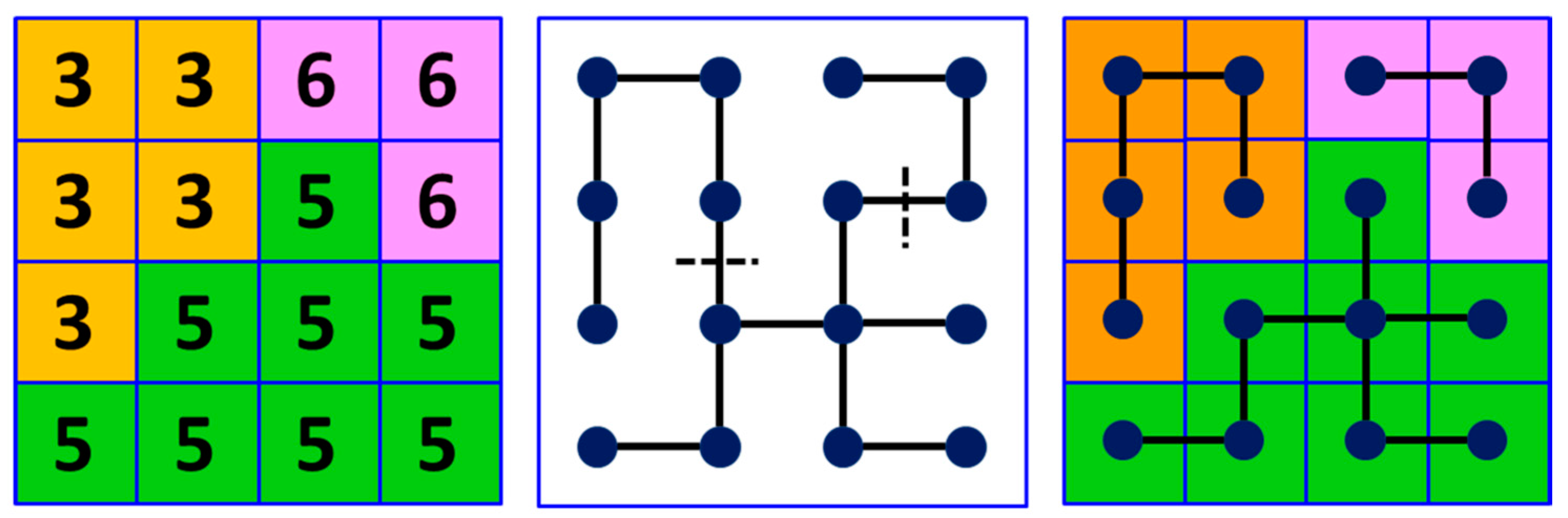
For a multi-spectral time series, the MST represents a connection of adjacent pixels that is globally optimized according to regions of spectral-temporal similarity based on DTW. The weights of edges indicate the degree of similarity between nodes. The edges with high weights can be removed to split the MST into a set of sub-trees that represent the different segments of the image. The removed edges in this study were identified using the spectral averaging method proposed by Lersch [86]. Figure 6 illustrates the principle of segmentation based on MST.
3.4. Spectral-Temporal-Spatial (STS) Classification Method
Our proposed method extracts and combines the spectral-temporal and spatial characteristics of remote sensing images using all the available data. The workflow of the proposed time-series land cover classification method is shown in Figure 7. The proposed classification method consists of the following four steps. (1) Time-series data are constructed based on the spectral-temporal arrangement. Then the similarity measure matrix is calculated by computing the DTW distance between pixels using all the available data (Section 3.1). (2) The spectral-temporal feature vectors extracted by the LE-DTW DR method (using the DTW similarity matrix to construct an adjacency graph) are classified to create a pixel-based classification map (Section 3.2). (3) A segmentation map is obtained by the MST-DTW method (an MST is created from a weighted graph based on the DTW similarity matrix; Section 3.3). (4) Spatial regularization is the strategy employed to combine the spectral-temporal and spatial features. In this step, majority voting [47,87] based on the segmentation map is utilized to post-process the pixel-based classification map. Finally, a land cover map is obtained based on the spectral-temporal-spatial (STS) classification method.
4. Experiments
A series of quantitative classification experiments were undertaken in each study area to verify the performance of the proposed method. Five classification methods were used for comparison, as shown in Table 1. The reasons for choosing these five methods are as follows. First, LE-DTW and STS are the methods proposed in this paper. The comparison of these two methods is to illustrate whether spatial information is useful for improving the accuracy of time-series land cover classification. Second, principal component analysis (PCA) is a typical linear DR method [44], and is compared to LE-DTW to explore the internal structure of satellite time-series data. Third, LE-SAM-R is a refined LE algorithm using the spectral angle mapper (SAM) with satellite time-series data after temporal interpolation [39]. We compared it with LE-DTW to illustrate which metric is more effective for satellite time-series data mining. Fourth, temporal interpolation (TI) only needs to interpolate the original time series data without DR, and then the interpolated data is directly input to the classifier to obtain the classification results. It is compared with LE-DTW to show whether there is a large amount of data redundancy in satellite images time series.
Because all of TI, PCA and LE-SAM-R require cloud-free land surface observations, we use temporal interpolation with the raw data using data from earlier and later dates. Specifically, if the band values for a pixel were covered by clouds on a certain date, these values were replaced by a temporally adjacent data point or the average of two temporally adjacent measurements if both the prior and following points are available.
Two popular supervised classifier random forests (RFs) [88] and support vector machine (SVM) [89,90] were used to generate pixel-based classification maps in experiments. The RF classifier is composed of multiple tree classifiers. In addition, each tree classifier casts an equal vote to choose the most popular classification of the input vector [91,92]. A total of 500 trees were built using RFs in this paper. In addition, the SVM classifier with a radial basis function (RBF) kernel was performed by using LIBSVM [93].
The same parameter settings were adopted for all three sets of experiments. Training data and testing data for classification in the three study areas were extracted from the 2014 CDL. In each study area, only the classes which covering over 2% on the CDL data were considered. In addition, 1% of the CDL pixels were randomly selected as training samples and the rest of pixels were used as testing data. A total of 1600, 1000, and 1250 training pixels were used for the Illinois, South Dakota, and Texas study areas, respectively. The traditional classification accuracy statistics obtained from confusion matrices, including the overall and single-class accuracies and kappa index were used to evaluate the performance of classification [3,94]. Sensitivity to training data with different proportions was also undertaken (take RF classifier as an example) by selecting at random from 0.1% to 10% of the CDL pixels in three study areas. To ensure the reliability of the results, all the experiments were repeated 10 times.
4.1. Performance of RF and SVM in Five Classification Methods
The classification results and the classification “stability” for the five classification methods combined with RF classifier and SVM classifier is illustrated in this section. The mean overall accuracies and kappa index values of five classification methods combined with two classifiers using 1% CDL training data are shown in Table 2. Comparing the two classifiers from the table, we can see that both RF and SVM classifier had similar overall accuracy and kappa index for each classification method in all three study areas. The maximum difference of overall accuracy using RF classifier and SVM classifier for TI, PCA, LE-SAM-R, LE-DTW and STS method in three study areas were 1.93%, 1.53%, 2.66%, 3.22% and 0.63%, respectively, and the corresponding difference of kappa index were 0.0217, 0.0857, 0.0395, 0.0456 and 0.0107. It is worth noting that, in the STS classification method, the difference of overall classification accuracy of two classifiers in three study areas were 0.51%, 0.52% and 0.63%, respectively, and the corresponding difference of kappa index were 0.0096, 0.0079, and 0.0107. Obviously, the performance of the two classifiers are most similar in the STS classification method, meaning that that method is more stable than the other four classification methods.
4.2. Satellite Image Time Series Data Redundancy
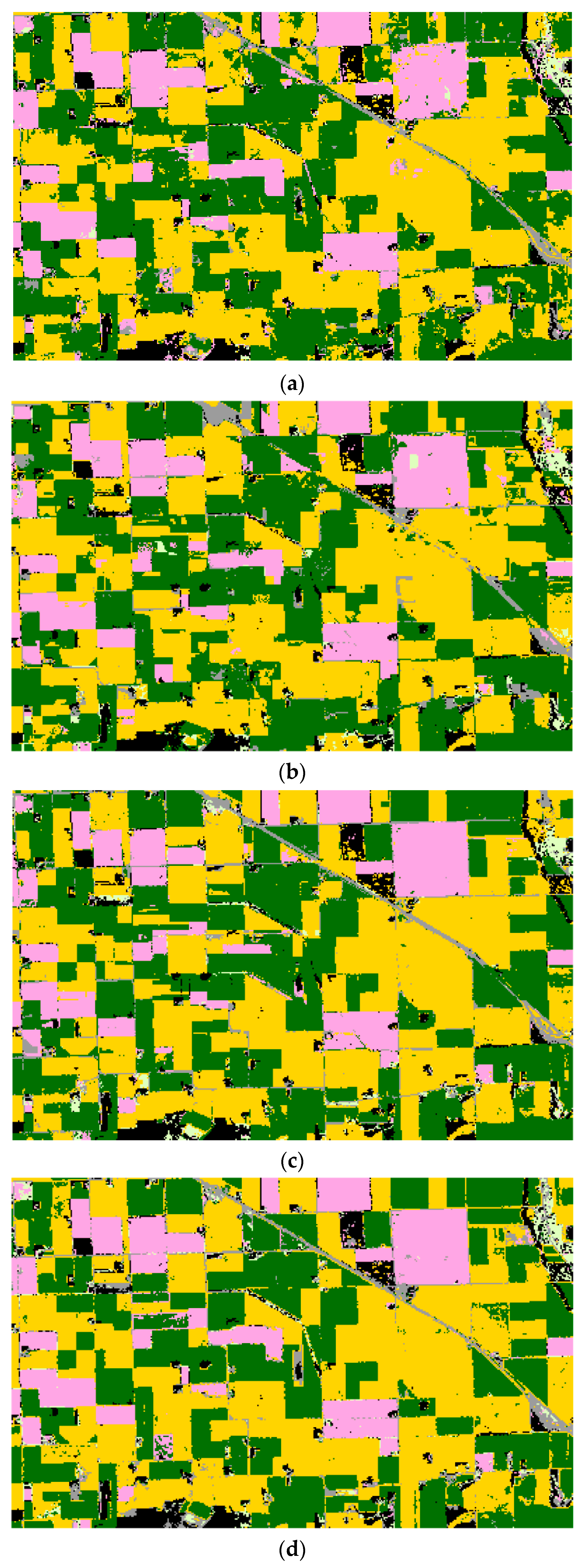
The mean overall accuracies and kappa index values of the TI and LE-DTW classification results using 1% CDL training data are shown in Table 2. The overall classification accuracy of the LE-DTW method is at least 2.72%, 1.77% and 8.40% higher than that of TI in Illinois, South Dakota, and Texas study areas, respectively. In addition, the kappa index of the LE-DTW method are raised more than 0.0658, 0.0325 and 0.1210 compared to the TI method in three study areas. Classification maps constructed using the TI and LE-DTW methods combined with RF classifier in three study areas are shown in Figure 8a,d, Figure 9a,d and Figure 10a,d. Table 3 and Table 4 summarize the mean producer’s and user’s accuracies for classification based on the TI and LE-DTW methods combined with RF classifier for each major crop category, respectively. The producer’s accuracy indicates the probability that a pixel is classified correctly, which equal the ratio of all the pixels classified correctly in a class to the sum of true reference pixels for that class [95]. The user’s accuracy indicates the probability that a pixel is classified to a specific class, which equal the ratio of all the pixels classified correctly in a class to the sum of all of the pixels allocated to that class [95]. The producer’s and user’s accuracies of TI method for most of the categories in the three study areas were significantly lower than those of the LE-DTW, especially in the CDL classes covering less than 10% of each study area. For example, the producer’s and user’s accuracies of the Illinois grass/pasture class (4.6% of the study area), the South Dakota developed/open space class (5.67% of the study area), and the Texas sorghum class (5.36% of the study area) in the TI method were 25.71%, 9.08% and 31.44% less than those of the LE-DTW method, respectively.
For satellite image time series, the classification accuracy of the data after DR is higher than that of the data without DR. Possible reasons are as follows. First, the time series data contains data redundancy, which cause the Hughes phenomenon [42]. Second, the temporal interpolation for time series data brings new error, especially the continuous temporal data are unavailable. Third, LE-DTW method provides dimensionality-reduced data that have desirable classification properties. Therefore, prior to land cover classification, it is appropriate to apply the DR techniques to satellite image time series.
4.3. Satellite Image Time Series Nonlinear Characteristics
The mean overall accuracies and kappa index values of the PCA and LE-DTW classification results using 1% CDL training data are shown in Table 2. The overall classification accuracy of the LE-DTW method combined with RF classifier or SVM classifier is more than 6% greater than that of PCA in all study areas, and its kappa index is also higher than that of PCA by more than 0.04. Classification maps constructed using the PCA methods combined with RF classifier in three study areas are shown in Figure 8b, Figure 9b and Figure 10b. Table 5 summarize the mean producer’s and user’s accuracies of classification based on the PCA methods combined with RF classifier for each major crop category. For the PCA DR method, the producer’s and user’s accuracies exceeded 76%, 86%, and 50% for all CDL classes covering more than 10% of each study area in Illinois, South Dakota, and Texas, respectively. However, the producer’s and user’s accuracies of the Illinois developed/open space class (5.29% of the study area), the South Dakota grass/pasture class (2.10% of the study area) and the Texas developed/open space class (4.92% of the study area) ranged from only 11% to 45%. For developed/open space class and grass/pasture class, the main reason for the low accuracy include two aspects. One is the small covering area resulting in the small size of the training sample, which means that it is difficult to establish reasonable classification rules when training classifiers. Another is that these natural land and vegetation classes have less pronounced phenology characteristics than the cropland classes.
For the LE-DTW method, the producer’s and user’s accuracies for all the categories in the three study areas were significantly higher than those of the PCA. This was to be expected, because satellite image time series have intrinsic nonlinear characteristics. Thus, LE-DTW, as a nonlinear DR method, is better suited than the linear DR method for solving the high dimensionality problem of satellite image time series. In addition, multi-spectral time-series data require cloud removal before PCA DR. Error generated by this pre-processing may be another reason that PCA has lower accuracy than LE-DTW.
4.4. Satellite Image Time Series Metric
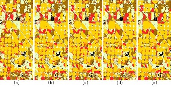
The mean overall accuracies and kappa index values of the LE-SAM-R classification results generated using 1% CDL training data are shown in Table 2. The overall classification accuracies and kappa index values of the LE-SAM-R method were lower than those of LE-DTW in all the three study areas. The largest relative improvement using the LE-DTW method was in the Texas study area. LE-DTW combined with RF classifier had a 3.26% greater overall accuracy and a 0.0450 increase in kappa index than LE-SAM-R combined with RF classifier. The classification maps for the LE-SAM-R method combined with RF classifier in the three study areas are shown in Figure 8c, Figure 9c and Figure 10c. Table 6 summarizes the mean producer and user accuracies of the classification based on the LE-SAM-R method combined with RF classifier for each major crop category. The producer and user accuracies exceeded 81%, 88%, and 70% for all CDL classes covering more than 10% of the study area in Illinois, South Dakota, and Texas, respectively. However, the producer’s accuracies of LE-SAM-R for most categories were also lower than those of the LE-DTW method.
These results suggest that the DTW distance is better suited for similarity measurement of multi-spectral time-series data than the SAM distance. The DTW metric ensures that all the data from cloudless regions in each temporal image are used. This is of great importance to those sensors that have low-frequency observations. It is worth noting that the LE-DTW method does not need to reconstruct the value of the data in the cloud-covered regions, whereas the LE-SAM-R method requires this reconstruction process. In other words, the LE-DTW method uses all the available data directly. Therefore, the LE-DTW method is a dimensionality reduction method which is more suitable for satellite image time series data.
4.5. Satellite Image Time Series Spatial Features
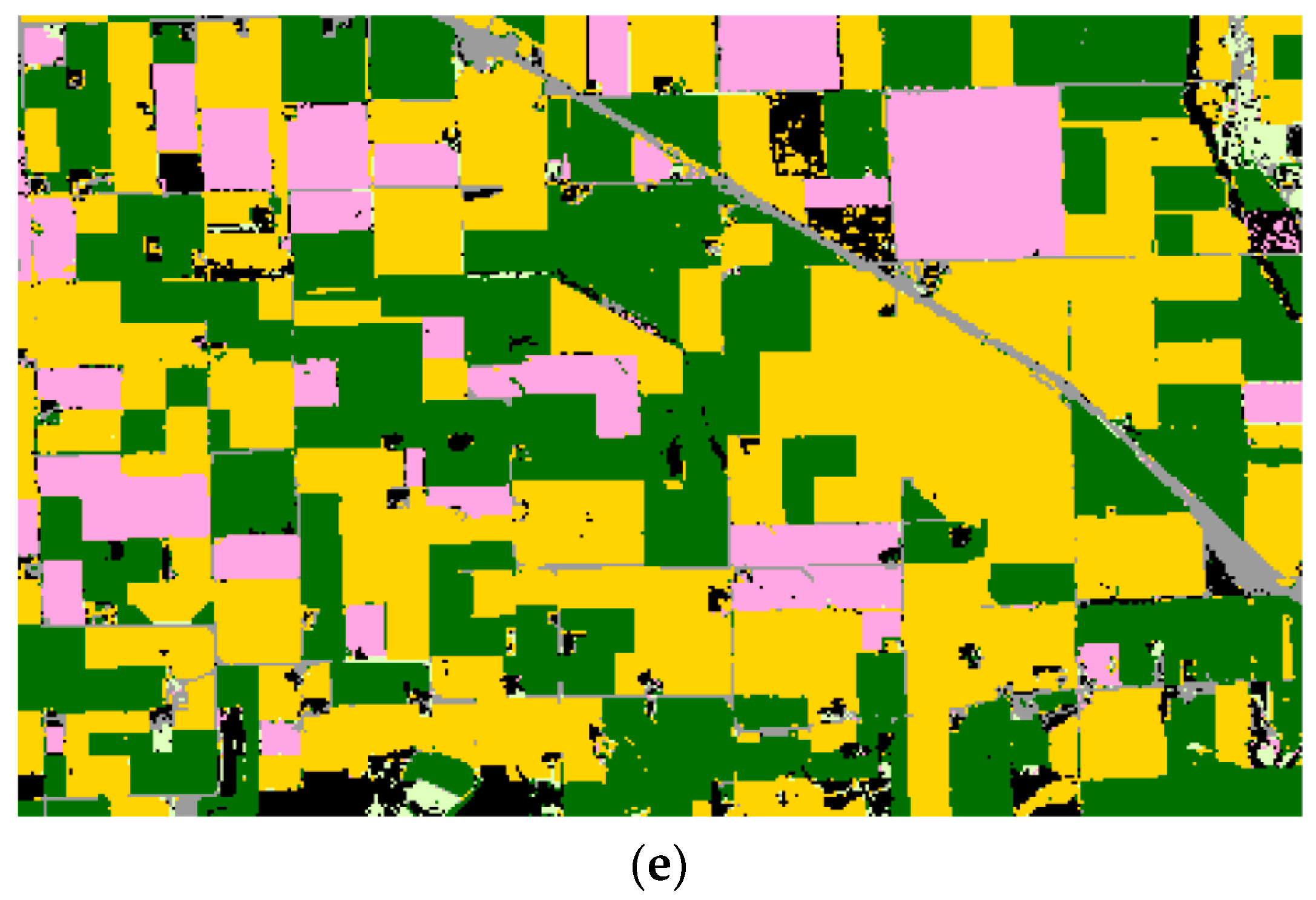
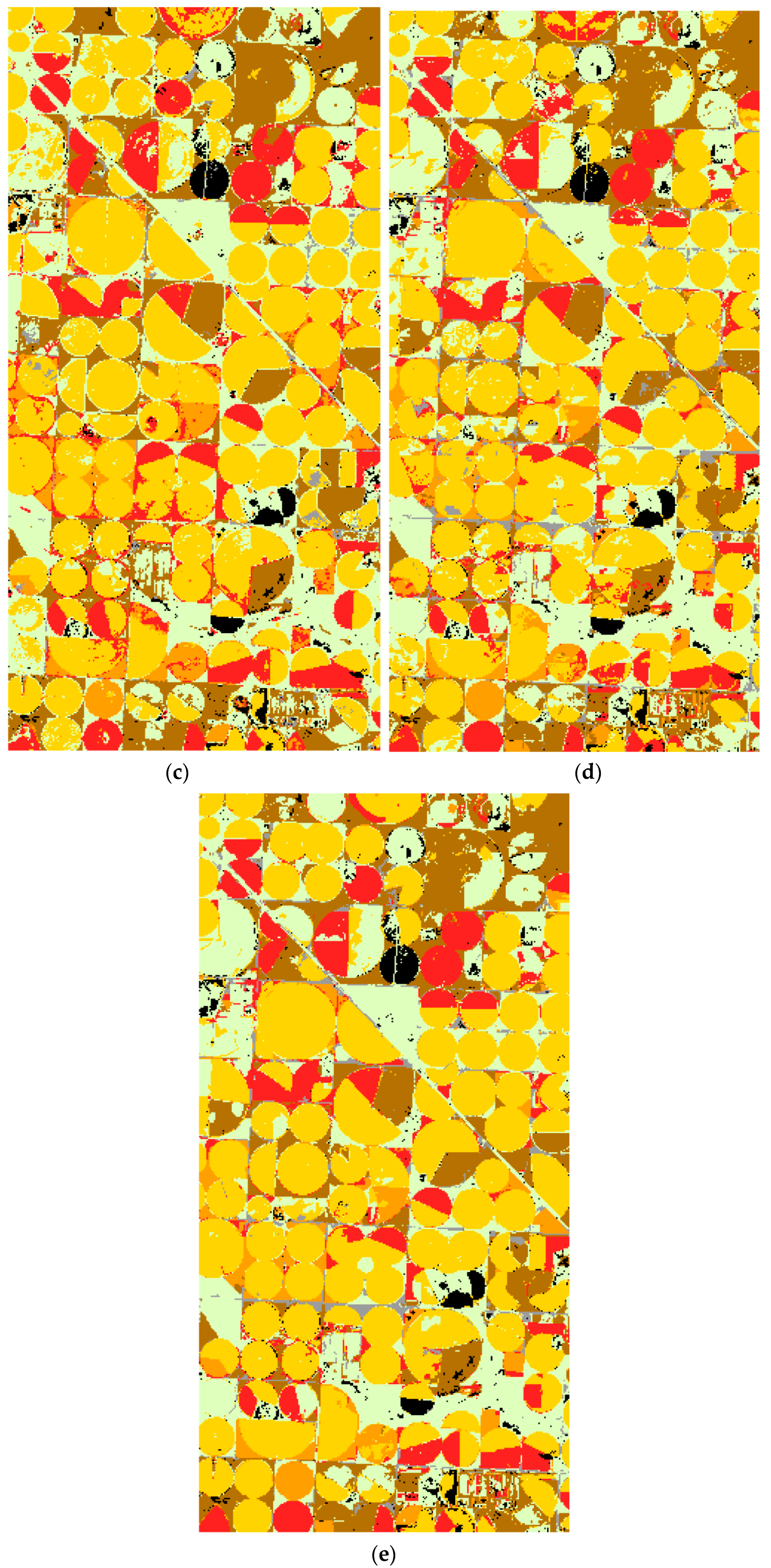
The mean overall accuracies and kappa index values of the STS classification results generated using 1% CDL training data are shown in Table 2. The STS method provides unambiguously higher overall classification accuracies than LE-DTW in most cases. It is worth noting that, compared to the LE-DTW method (combining RF classifier), the overall classification accuracies improved by 1.66%, 4.01%, and 1.13% in Illinois, South Dakota, and Texas study areas, respectively, using the STS method (combining RF classifier), while the corresponding kappa index values were enhanced by 0.0258, 0.0594 and 0.0136. Similarly, the performance of STS method combined with SVM classifier is better than that of LE-DTW method combined with SVM classifier. Classification maps generated using the STS method combined with RF classifier in the three study areas are shown in Figure 8e, Figure 9e and Figure 10e. Table 7 summarizes the mean producer and user accuracies of classification based on the STS method combined with RF classifier for each major crop category. Compared to the producer and user accuracies in Table 6, the corresponding accuracies stated in Table 7 were higher for the great majority of classes. Furthermore, for CDL classes covering less than 10% of each study area, the producer and user accuracies of the STS method were also greatly improved. For example, the producer’s accuracies of the Illinois developed/open space class (5.29% of the study area), the South Dakota developed/open space class (5.67% of the study area), and the Texas sorghum class (5.36% of the study area) in the STS method were 8.73%, 19.06% and 2.4% greater than those of the LE-DTW method, respectively.
These results show that the MST-DTW method can effectively extract spatial features from satellite image time series using all available data. The STS method combined with spatial information extracted by MST-DTW significantly improves the land cover classification accuracies of multi-spectral time-series data. STS can mine a variety of features from limited data for classification; therefore, it is particularly effective for remote sensing image time series with low temporal resolution.
4.6. Classification Sensitivity to the Amount of Training Data
Classification accuracy always directly depends on the amount of the training data [96]. Careful selection of training samples may help reduce the size of the training data without reducing supervised classification accuracy [97]. When using fewer training samples, a given classification accuracy should be capacitated by a more optimal classification method than a less one [39].
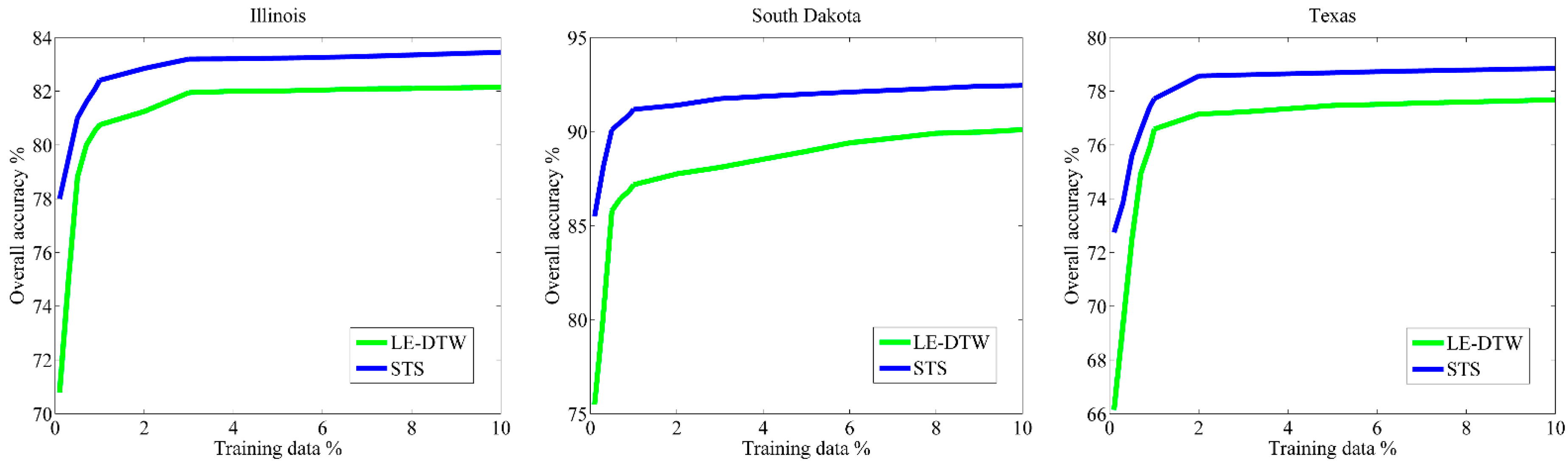
Figure 11 illustrates the overall classification accuracies provided by the LE-DTW (green) and STS (blue) using different percentages of training data. At each training percentage, a total of 10 independent classifications were performed. As can be seen from Figure 11, the overall classification accuracies of STS approach are consistently higher than the LE-DTW approach. Moreover, when using fewer training samples, the classification performances of STS method are more stable than that of LE-DTW method. Both the overall classification accuracies of STS approach and LE-DTW become stable when approximately 1% of the training samples are used. For each set of 10 classifications, the standard deviations of the overall classification accuracies are not illustrated. This is because the standard deviation for each set experiments were less than 1% except for the results using the 0.1% training data which were less than 2.1% in the three study areas. These results show that the STS method using spectral-temporal-spatial features is more optimal than the LE-DTW method using spectral-temporal features only.
5. Conclusions
Obtaining accurate and timely land cover maps is a difficult problem in remote sensing. Such maps require the mining of as much useful information as possible to improve land cover classification accuracy based on limited data. In this study, a novel method is developed for land cover classification using spectral-temporal-spatial data at an annual scale, assuming there is no land cover change within 1 year. This approach utilizes all the available multi-spectral time-series data to construct a graph based on the DTW similarity measure, and then utilizes graph theory-based dimensionality reduction and segmentation methods to extract spectral-temporal features and spatial features for identification and optimization of land cover classes. In addition, the proposed method is an automated classification method, and requires few training samples to perform well. These advantages are significant because land cover classification is labor-intensive and difficult to automate [98,99]. Therefore, the classification method introduced in this paper should prove useful for improving the accuracy and reducing the mapping period for land cover classification. The proposed method was applied to Landsat multi-spectral reflectance time-series data, which has a resample period of 16 days. A series of supervised classification experiments using USDA CDL land cover maps as reference data were undertaken in three study areas with land cover complexity and different amounts of invalid data in the United States.
Although the STS classification method provided the anticipated classification results in this study, the computation required for the LE-DTW method in the STS system increases geometrically with the spatial dimensions of the image. In fact, this problem occurs in most manifold learning DR algorithms [100,101,102,103,104]. This is an issue, especially when manifold learning DR algorithms are applied to land cover classification at continental to global scale [13,105]. Due to the complexity of the MST-DTW algorithm, it is mainly implemented by building a DTW similarity measure matrix in the same manner as LE-DTW, and therefore MST-DTW does not significantly increase the computational intensity of the STS system. Reducing its computational requirements is a direction for future research. This could be accomplished, for example, by employing the landmark points strategy [106] developed for the ISOMAP (isometric mapping) global nonlinear DR method [67,107,108], GPU (Graphics Processing Unit) enhanced computing [109], and the STS method to classify and then merge image subsets. In addition, we are now conducting experiments using long-term multi-spectral time-series data with invalid values for land cover change detection with spectral-temporal-spatial features extracted from the STS system.
Acknowledgments
The work of this paper was supported by the National Key Research and Development Program of China under grant number of 2016YFC0501301 and the National Natural Science Foundation of China under grant number of 51779117.
Author Contributions
Yongguang Zhai and Lei Hao wrote the paper. Zhongyi Qu did the data pre-processing for Section 4.
Conflicts of Interest
The authors declare no conflict of interest.
References
- Feddema, J.J.; Oleson, K.W.; Bonan, G.B.; Mearns, L.O.; Buja, L.E.; Meehl, G.A.; Washington, W.M. The importance of land-cover change in simulating future climates. Science 2005, 310, 1674–1678. [Google Scholar] [CrossRef] [PubMed]
- Wulder, M.A.; White, J.C.; Goward, S.N.; Masek, J.G.; Irons, J.R.; Herold, M.; Cohen, W.B.; Loveland, T.R.; Woodcock, C.E. Landsat continuity: Issues and opportunities for land cover monitoring. Remote Sens. Environ. 2008, 112, 955–969. [Google Scholar] [CrossRef]
- Foody, G.M. Status of land cover classification accuracy assessment. Remote Sens. Environ. 2002, 80, 185–201. [Google Scholar] [CrossRef]
- Chen, J.; Chen, J.; Liao, A.; Cao, X.; Chen, L.; Chen, X.; He, C.; Han, G.; Peng, S.; Lu, M. Global land cover mapping at 30 m resolution: A POK-based operational approach. ISPRS J. Photogramm. Remote Sens. 2015, 103, 7–27. [Google Scholar] [CrossRef]
- Gong, P.; Wang, J.; Yu, L.; Zhao, Y.; Zhao, Y.; Liang, L.; Niu, Z.; Huang, X.; Fu, H.; Liu, S. Finer resolution observation and monitoring of global land cover: First mapping results with Landsat TM and ETM+ data. Int. J. Remote Sens. 2013, 34, 2607–2654. [Google Scholar] [CrossRef]
- Verburg, P.H.; Neumann, K.; Nol, L. Challenges in using land use and land cover data for global change studies. Glob. Chang. Biol. 2011, 17, 974–989. [Google Scholar] [CrossRef] [Green Version]
- Ewert, F.; Rounsevell, M.; Reginster, I.; Metzger, M.; Leemans, R. Future scenarios of European agricultural land use: I. Estimating changes in crop productivity. Agric. Ecosyst. Environ. 2005, 107, 101–116. [Google Scholar] [CrossRef]
- Foley, J.A.; DeFries, R.; Asner, G.P.; Barford, C.; Bonan, G.; Carpenter, S.R.; Chapin, F.S.; Coe, M.T.; Daily, G.C.; Gibbs, H.K. Global consequences of land use. Science 2005, 309, 570–574. [Google Scholar] [CrossRef] [PubMed]
- Gómez, C.; White, J.C.; Wulder, M.A. Optical remotely sensed time series data for land cover classification: A review. ISPRS J. Photogramm. Remote Sens. 2016, 116, 55–72. [Google Scholar] [CrossRef]
- Grekousis, G.; Mountrakis, G.; Kavouras, M. An overview of 21 global and 43 regional land-cover mapping products. Int. J. Remote Sens. 2015, 36, 5309–5335. [Google Scholar] [CrossRef]
- Belward, A.S.; Estes, J.E.; Kline, K.D. The IGBP-DIS global 1-km land-cover data set DISCover: A project overview. Photogramm. Eng. Remote Sens. 1999, 65, 1013–1020. [Google Scholar]
- Hansen, M.C.; Loveland, T.R. A review of large area monitoring of land cover change using Landsat data. Remote Sens. Environ. 2012, 122, 66–74. [Google Scholar] [CrossRef]
- Friedl, M.A.; Sulla-Menashe, D.; Tan, B.; Schneider, A.; Ramankutty, N.; Sibley, A.; Huang, X. MODIS Collection 5 global land cover: Algorithm refinements and characterization of new datasets. Remote Sens. Environ. 2010, 114, 168–182. [Google Scholar] [CrossRef]
- Bartholomé, E.; Belward, A. GLC2000: A new approach to global land cover mapping from Earth observation data. Int. J. Remote Sens. 2005, 26, 1959–1977. [Google Scholar] [CrossRef]
- Müller, H.; Rufin, P.; Griffiths, P.; Siqueira, A.J.B.; Hostert, P. Mining dense Landsat time series for separating cropland and pasture in a heterogeneous Brazilian savanna landscape. Remote Sens. Environ. 2015, 156, 490–499. [Google Scholar] [CrossRef]
- Waldner, F.; Canto, G.S.; Defourny, P. Automated annual cropland mapping using knowledge-based temporal features. ISPRS J. Photogramm. Remote Sens. 2015, 110, 1–13. [Google Scholar] [CrossRef]
- Sexton, J.O.; Urban, D.L.; Donohue, M.J.; Song, C. Long-term land cover dynamics by multi-temporal classification across the Landsat-5 record. Remote Sens. Environ. 2013, 128, 246–258. [Google Scholar] [CrossRef]
- Yuan, F.; Sawaya, K.E.; Loeffelholz, B.C.; Bauer, M.E. Land cover classification and change analysis of the Twin Cities (Minnesota) Metropolitan Area by multitemporal Landsat remote sensing. Remote Sens. Environ. 2005, 98, 317–328. [Google Scholar] [CrossRef]
- Clark, M.L.; Aide, T.M.; Grau, H.R.; Riner, G. A scalable approach to mapping annual land cover at 250 m using MODIS time series data: A case study in the Dry Chaco ecoregion of South America. Remote Sens. Environ. 2010, 114, 2816–2832. [Google Scholar] [CrossRef]
- Jia, K.; Liang, S.; Zhang, N.; Wei, X.; Gu, X.; Zhao, X.; Yao, Y.; Xie, X. Land cover classification of finer resolution remote sensing data integrating temporal features from time series coarser resolution data. ISPRS J. Photogramm. Remote Sens. 2014, 93, 49–55. [Google Scholar] [CrossRef]
- Hansen, M.C.; Egorov, A.; Roy, D.P.; Potapov, P.; Ju, J.; Turubanova, S.; Kommareddy, I.; Loveland, T.R. Continuous fields of land cover for the conterminous United States using Landsat data: First results from the Web-Enabled Landsat Data (WELD) project. Remote Sens. Lett. 2011, 2, 279–288. [Google Scholar] [CrossRef]
- Ju, J.; Roy, D.P. The availability of cloud-free Landsat ETM+ data over the conterminous United States and globally. Remote Sens. Environ. 2008, 112, 1196–1211. [Google Scholar] [CrossRef]
- Zhu, Z.; Woodcock, C.E. Continuous change detection and classification of land cover using all available Landsat data. Remote Sens. Environ. 2014, 144, 152–171. [Google Scholar] [CrossRef]
- Dong, J.; Xiao, X.; Kou, W.; Qin, Y.; Zhang, G.; Li, L.; Jin, C.; Zhou, Y.; Wang, J.; Biradar, C. Tracking the dynamics of paddy rice planting area in 1986–2010 through time series Landsat images and phenology-based algorithms. Remote Sens. Environ. 2015, 160, 99–113. [Google Scholar] [CrossRef]
- Inglada, J.; Vincent, A.; Arias, M.; Tardy, B.; Morin, D.; Rodes, I. Operational high resolution land cover map production at the country scale using satellite image time series. Remote Sens. 2017, 9, 95. [Google Scholar] [CrossRef]
- Sakamoto, T.; Yokozawa, M.; Toritani, H.; Shibayama, M.; Ishitsuka, N.; Ohno, H. A crop phenology detection method using time-series MODIS data. Remote Sens. Environ. 2005, 96, 366–374. [Google Scholar] [CrossRef]
- Roerink, G.; Menenti, M.; Verhoef, W. Reconstructing cloudfree NDVI composites using Fourier analysis of time series. Int. J. Remote Sens. 2000, 21, 1911–1917. [Google Scholar] [CrossRef]
- Schaaf, C.B.; Gao, F.; Strahler, A.H.; Lucht, W.; Li, X.; Tsang, T.; Strugnell, N.C.; Zhang, X.; Jin, Y.; Muller, J.-P. First operational BRDF, albedo nadir reflectance products from MODIS. Remote Sens. Environ. 2002, 83, 135–148. [Google Scholar] [CrossRef]
- Pan, Z.; Huang, J.; Zhou, Q.; Wang, L.; Cheng, Y.; Zhang, H.; Blackburn, G.A.; Yan, J.; Liu, J. Mapping crop phenology using NDVI time-series derived from HJ-1 A/B data. Int. J. Appl. Earth Obs. Geoinf. 2015, 34, 188–197. [Google Scholar] [CrossRef]
- King, L.; Adusei, B.; Stehman, S.V.; Potapov, P.V.; Song, X.-P.; Krylov, A.; Di Bella, C.; Loveland, T.R.; Johnson, D.M.; Hansen, M.C. A multi-resolution approach to national-scale cultivated area estimation of soybean. Remote Sens. Environ. 2017, 195, 13–29. [Google Scholar] [CrossRef]
- Byrne, G.; Crapper, P.; Mayo, K. Monitoring land-cover change by principal component analysis of multitemporal Landsat data. Remote Sens. Environ. 1980, 10, 175–184. [Google Scholar] [CrossRef]
- Collins, J.B.; Woodcock, C.E. An assessment of several linear change detection techniques for mapping forest mortality using multitemporal Landsat TM data. Remote Sens. Environ. 1996, 56, 66–77. [Google Scholar] [CrossRef]
- Löw, F.; Michel, U.; Dech, S.; Conrad, C. Impact of feature selection on the accuracy and spatial uncertainty of per-field crop classification using support vector machines. ISPRS J. Photogramm. Remote Sens. 2013, 85, 102–119. [Google Scholar] [CrossRef]
- Singh, A. Review article digital change detection techniques using remotely-sensed data. Int. J. Remote Sens. 1989, 10, 989–1003. [Google Scholar] [CrossRef]
- Tewkesbury, A.P.; Comber, A.J.; Tate, N.J.; Lamb, A.; Fisher, P.F. A critical synthesis of remotely sensed optical image change detection techniques. Remote Sens. Environ. 2015, 160, 1–14. [Google Scholar] [CrossRef]
- Kuncheva, L.I.; Faithfull, W.J. PCA feature extraction for change detection in multidimensional unlabeled data. IEEE Trans. Neural Netw. Learn. Syst. 2014, 25, 69–80. [Google Scholar] [CrossRef] [PubMed]
- Deng, J.; Wang, K.; Deng, Y.; Qi, G. PCA-based land-use change detection and analysis using multitemporal and multisensor satellite data. Int. J. Remote Sens. 2008, 29, 4823–4838. [Google Scholar] [CrossRef]
- Deng, J.S.; Wang, K.; Hong, Y.; Qi, J.G. Spatio-temporal dynamics and evolution of land use change and landscape pattern in response to rapid urbanization. Landsc. Urban Plan. 2009, 92, 187–198. [Google Scholar] [CrossRef]
- Yan, L.; Roy, D. Improved time series land cover classification by missing-observation-adaptive nonlinear dimensionality reduction. Remote Sens. Environ. 2015, 158, 478–491. [Google Scholar] [CrossRef]
- Peña, M.; Brenning, A. Assessing fruit-tree crop classification from Landsat-8 time series for the Maipo Valley, Chile. Remote Sens. Environ. 2015, 171, 234–244. [Google Scholar] [CrossRef]
- Harsanyi, J.C.; Chang, C.-I. Hyperspectral image classification and dimensionality reduction: An orthogonal subspace projection approach. IEEE Trans. Geosci. Remote Sens. 1994, 32, 779–785. [Google Scholar] [CrossRef]
- Hughes, G. On the mean accuracy of statistical pattern recognizers. IEEE Trans. Inf. Theory 1968, 14, 55–63. [Google Scholar] [CrossRef]
- Lunga, D.; Prasad, S.; Crawford, M.M.; Ersoy, O. Manifold-learning-based feature extraction for classification of hyperspectral data: A review of advances in manifold learning. IEEE Signal Process. Mag. 2014, 31, 55–66. [Google Scholar] [CrossRef]
- Rodarmel, C.; Shan, J. Principal component analysis for hyperspectral image classification. Surv. Land Inf. Sci. 2002, 62, 115–122. [Google Scholar]
- Kuo, B.-C.; Landgrebe, D.A. Nonparametric weighted feature extraction for classification. IEEE Trans. Geosci. Remote Sens. 2004, 42, 1096–1105. [Google Scholar]
- Jia, X.; Kuo, B.-C.; Crawford, M.M. Feature mining for hyperspectral image classification. Proc. IEEE 2013, 101, 676–697. [Google Scholar] [CrossRef]
- Fauvel, M.; Tarabalka, Y.; Benediktsson, J.A.; Chanussot, J.; Tilton, J.C. Advances in spectral-spatial classification of hyperspectral images. Proc. IEEE 2013, 101, 652–675. [Google Scholar] [CrossRef]
- Tarabalka, Y.; Benediktsson, J.A.; Chanussot, J. Spectral–spatial classification of hyperspectral imagery based on partitional clustering techniques. IEEE Trans. Geosci. Remote Sens. 2009, 47, 2973–2987. [Google Scholar] [CrossRef]
- Tarabalka, Y.; Benediktsson, J.A.; Chanussot, J.; Tilton, J.C. Multiple spectral–spatial classification approach for hyperspectral data. IEEE Trans. Geosci. Remote Sens. 2010, 48, 4122–4132. [Google Scholar] [CrossRef]
- Li, J.; Bioucas-Dias, J.M.; Plaza, A. Spectral–spatial hyperspectral image segmentation using subspace multinomial logistic regression and Markov random fields. IEEE Trans. Geosci. Remote Sens. 2012, 50, 809–823. [Google Scholar] [CrossRef]
- Benediktsson, J.A.; Palmason, J.A.; Sveinsson, J.R. Classification of hyperspectral data from urban areas based on extended morphological profiles. IEEE Trans. Geosci. Remote Sens. 2005, 43, 480–491. [Google Scholar] [CrossRef]
- Blaschke, T. Object based image analysis for remote sensing. ISPRS J. Photogramm. Remote Sens. 2010, 65, 2–16. [Google Scholar] [CrossRef]
- Gong, P.; Marceau, D.J.; Howarth, P.J. A comparison of spatial feature extraction algorithms for land-use classification with SPOT HRV data. Remote Sens. Environ. 1992, 40, 137–151. [Google Scholar] [CrossRef]
- Dey, V.; Zhang, Y.; Zhong, M. A review on image segmentation techniques with remote sensing perspective. Int. Arch. Photogramm. Remote Sens. 2010, XXXVIII, 31–42. [Google Scholar]
- Knight, E.J.; Kvaran, G. Landsat-8 operational land imager design, characterization and performance. Remote Sens. 2014, 6, 10286–10305. [Google Scholar] [CrossRef]
- Loveland, T.R.; Dwyer, J.L. Landsat: Building a strong future. Remote Sens. Environ. 2012, 122, 22–29. [Google Scholar] [CrossRef]
- Morfitt, R.; Barsi, J.; Levy, R.; Markham, B.; Micijevic, E.; Ong, L.; Scaramuzza, P.; Vanderwerff, K. Landsat-8 Operational Land Imager (OLI) radiometric performance on-orbit. Remote Sens. 2015, 7, 2208–2237. [Google Scholar] [CrossRef]
- Roy, D.P.; Wulder, M.; Loveland, T.; Woodcock, C.; Allen, R.; Anderson, M.; Helder, D.; Irons, J.; Johnson, D.; Kennedy, R. Landsat-8: Science and product vision for terrestrial global change research. Remote Sens. Environ. 2014, 145, 154–172. [Google Scholar] [CrossRef]
- Han, W.; Yang, Z.; Di, L.; Mueller, R. CropScape: A Web service based application for exploring and disseminating US conterminous geospatial cropland data products for decision support. Comput. Electron. Agric. 2012, 84, 111–123. [Google Scholar] [CrossRef]
- Boryan, C.; Yang, Z.; Mueller, R.; Craig, M. Monitoring US agriculture: The US department of agriculture, national agricultural statistics service, cropland data layer program. Geocarto Int. 2011, 26, 341–358. [Google Scholar] [CrossRef]
- Masek, J.G.; Vermote, E.F.; Saleous, N.E.; Wolfe, R.; Hall, F.G.; Huemmrich, K.F.; Gao, F.; Kutler, J.; Lim, T.-K. A Landsat surface reflectance dataset for North America, 1990–2000. IEEE Geosci. Remote Sens. Lett. 2006, 3, 68–72. [Google Scholar] [CrossRef]
- Berndt, D.J.; Clifford, J. Using dynamic time warping to find patterns in time series. In Proceedings of the KDD Workshop, Seattle, WA, USA, 31 July–1 August 1994; pp. 359–370. [Google Scholar]
- Sakoe, H.; Chiba, S. Dynamic programming algorithm optimization for spoken word recognition. IEEE Trans. Acoust. Speech Signal Process. 1978, 26, 43–49. [Google Scholar] [CrossRef]
- Petitjean, F.; Inglada, J.; Gançarski, P. Satellite image time series analysis under time warping. IEEE Trans. Geosci. Remote Sens. 2012, 50, 3081–3095. [Google Scholar] [CrossRef]
- Jeong, Y.-S.; Jeong, M.K.; Omitaomu, O.A. Weighted dynamic time warping for time series classification. Pattern Recognit. 2011, 44, 2231–2240. [Google Scholar] [CrossRef]
- Bachmann, C.M.; Ainsworth, T.L.; Fusina, R.A. Exploiting manifold geometry in hyperspectral imagery. IEEE Trans. Geosci. Remote Sens. 2005, 43, 441–454. [Google Scholar] [CrossRef]
- Bachmann, C.M.; Ainsworth, T.L.; Fusina, R.A. Improved manifold coordinate representations of large-scale hyperspectral scenes. IEEE Trans. Geosci. Remote Sens. 2006, 44, 2786–2803. [Google Scholar] [CrossRef]
- Crawford, M.M.; Ma, L.; Kim, W. Exploring nonlinear manifold learning for classification of hyperspectral data. In Optical Remote Sensing; Springer: New York, NY, USA, 2011; pp. 207–234. [Google Scholar]
- Bioucas-Dias, J.M.; Plaza, A.; Camps-Valls, G.; Scheunders, P.; Nasrabadi, N.; Chanussot, J. Hyperspectral remote sensing data analysis and future challenges. IEEE Geosci. Remote Sens. Mag. 2013, 1, 6–36. [Google Scholar] [CrossRef]
- Tenenbaum, J.B.; De Silva, V.; Langford, J.C. A global geometric framework for nonlinear dimensionality reduction. Science 2000, 290, 2319–2323. [Google Scholar] [CrossRef] [PubMed]
- Belkin, M.; Niyogi, P. Laplacian eigenmaps and spectral techniques for embedding and clustering. In Proceedings of the NIPS, Vancouver, BC, Canada, 3–8 December 2001; pp. 585–591. [Google Scholar]
- Belkin, M.; Niyogi, P. Laplacian eigenmaps for dimensionality reduction and data representation. Neural Comput. 2003, 15, 1373–1396. [Google Scholar] [CrossRef]
- Bengio, Y.; Paiement, J.-F.; Vincent, P.; Delalleau, O.; Le Roux, N.; Ouimet, M. Out-of-sample extensions for lle, isomap, mds, eigenmaps, and spectral clustering. Adv. Neural Inf. Process. Syst. 2004, 16, 177–184. [Google Scholar]
- Saul, L.K.; Weinberger, K.Q.; Ham, J.H.; Sha, F.; Lee, D.D. Spectral methods for dimensionality reduction. In Semi-supervised Learning; Chapelle, O., Scholkopf, B., Zien, A., Eds.; The MIT Press: Cambridge, MA, USA, 2006. [Google Scholar]
- Yan, S.; Xu, D.; Zhang, B.; Zhang, H.-J.; Yang, Q.; Lin, S. Graph embedding and extensions: A general framework for dimensionality reduction. IEEE Trans. Pattern Anal. Mach. Intell. 2007, 29, 40–51. [Google Scholar] [CrossRef] [PubMed]
- Zhai, Y.; Zhang, L.; Wang, N.; Guo, Y.; Cen, Y.; Wu, T.; Tong, Q. A modified locality-preserving projection approach for hyperspectral image classification. IEEE Geosci. Remote Sens. Lett. 2016, 13, 1059–1063. [Google Scholar] [CrossRef]
- Levina, E.; Bickel, P.J. Maximum likelihood estimation of intrinsic dimension. In Proceedings of the Advances in Neural Information Processing Systems, Vancouver, BC, Canada, 13–18 December 2004; pp. 777–784. [Google Scholar]
- Hasanlou, M.; Samadzadegan, F. Comparative study of intrinsic dimensionality estimation and dimension reduction techniques on hyperspectral images using K-NN classifier. IEEE Geosci. Remote Sens. Lett. 2012, 9, 1046–1050. [Google Scholar] [CrossRef]
- Sonka, M.; Hlavac, V.; Boyle, R. Image Processing, Analysis, and Machine Vision; Cengage Learning: Boston, MA, USA, 2014. [Google Scholar]
- Benz, U.C.; Hofmann, P.; Willhauck, G.; Lingenfelder, I.; Heynen, M. Multi-resolution, object-oriented fuzzy analysis of remote sensing data for GIS-ready information. ISPRS J. Photogramm. Remote Sens. 2004, 58, 239–258. [Google Scholar] [CrossRef]
- Peng, B.; Zhang, L.; Zhang, D. A survey of graph theoretical approaches to image segmentation. Pattern Recognit. 2013, 46, 1020–1038. [Google Scholar] [CrossRef]
- Zahn, C.T. Graph-theoretical methods for detecting and describing gestalt clusters. IEEE Trans. Comput. 1971, 100, 68–86. [Google Scholar] [CrossRef]
- Felzenszwalb, P.F.; Huttenlocher, D.P. Efficient graph-based image segmentation. Int. J. Comput. Vis. 2004, 59, 167–181. [Google Scholar] [CrossRef]
- Kruskal, J.B. On the shortest spanning subtree of a graph and the traveling salesman problem. Proc. Am. Math. Soc. 1956, 7, 48–50. [Google Scholar] [CrossRef]
- Prim, R.C. Shortest connection networks and some generalizations. Bell Syst. Tech. J. 1957, 36, 1389–1401. [Google Scholar] [CrossRef]
- Lersch, J.R.; Iverson, A.E.; Webb, B.N.; West, K.F. Segmentation of multiband imagery using minimum spanning trees. In Proceedings of the Aerospace/Defense Sensing and Controls, Orlando, FL, USA, 8–12 April 1996; pp. 10–18. [Google Scholar]
- Lam, L.; Suen, S. Application of majority voting to pattern recognition: An analysis of its behavior and performance. IEEE Trans. Syst. Man Cybern. Part A Syst. Hum. 1997, 27, 553–568. [Google Scholar] [CrossRef]
- Breiman, L. Random forests. Mach. Learn. 2001, 45, 5–32. [Google Scholar] [CrossRef]
- Mountrakis, G.; Im, J.; Ogole, C. Support vector machines in remote sensing: A review. ISPRS J. Photogramm. Remote Sens. 2011, 66, 247–259. [Google Scholar] [CrossRef]
- Cortes, C.; Vapnik, V. Support vector machine. Mach. Learn. 1995, 20, 273–297. [Google Scholar] [CrossRef]
- Pal, M. Random forest classifier for remote sensing classification. Int. J. Remote Sens. 2005, 26, 217–222. [Google Scholar] [CrossRef]
- Gislason, P.O.; Benediktsson, J.A.; Sveinsson, J.R. Random forests for land cover classification. Pattern Recognit. Lett. 2006, 27, 294–300. [Google Scholar] [CrossRef]
- Chang, C.-C.; Lin, C.-J. LIBSVM: A library for support vector machines. ACM Trans. Intell. Syst. Technol. 2011, 2, 27. [Google Scholar] [CrossRef]
- Congalton, R.G. A review of assessing the accuracy of classifications of remotely sensed data. Remote Sens. Environ. 1991, 37, 35–46. [Google Scholar] [CrossRef]
- Congalton, R.G.; Green, K. Assessing the Accuracy of Remotely Sensed Data: Principles and Practices; CRC Press: Boca Raton, FL, USA, 2008. [Google Scholar]
- Hsiao, L.-H.; Cheng, K.-S. Assessing Uncertainty in LULC Classification Accuracy by Using Bootstrap Resampling. Remote Sens. 2016, 8, 705. [Google Scholar] [CrossRef]
- Foody, G.M.; Mathur, A. Toward intelligent training of supervised image classifications: Directing training data acquisition for SVM classification. Remote Sens. Environ. 2004, 93, 107–117. [Google Scholar] [CrossRef]
- Townshend, J.R.; Masek, J.G.; Huang, C.; Vermote, E.F.; Gao, F.; Channan, S.; Sexton, J.O.; Feng, M.; Narasimhan, R.; Kim, D. Global characterization and monitoring of forest cover using Landsat data: Opportunities and challenges. Int. J. Digit. Earth 2012, 5, 373–397. [Google Scholar] [CrossRef]
- Di Gregorio, A. Land Cover Classification System: Classification Concepts and User Manual: LCCS; Food & Agriculture Org.: Quebec City, QC, Canada, 2005. [Google Scholar]
- Saul, L.K.; Roweis, S.T. Think globally, fit locally: Unsupervised learning of low dimensional manifolds. J. Mach. Learn. Res. 2003, 4, 119–155. [Google Scholar]
- Belkin, M.; Niyogi, P.; Sindhwani, V. Manifold regularization: A geometric framework for learning from labeled and unlabeled examples. J. Mach. Learn. Res. 2006, 7, 2399–2434. [Google Scholar]
- Zhang, Z.-Y.; Zha, H.-Y. Principal manifolds and nonlinear dimensionality reduction via tangent space alignment. J. Shanghai Univ. 2004, 8, 406–424. [Google Scholar] [CrossRef]
- Van Der Maaten, L.; Postma, E.; Van den Herik, J. Dimensionality reduction: A comparative. J. Mach. Learn. Res. 2009, 10, 66–71. [Google Scholar]
- Maaten, L.V.d.; Hinton, G. Visualizing data using t-SNE. J. Mach. Learn. Res. 2008, 9, 2579–2605. [Google Scholar]
- Hansen, M.; Egorov, A.; Potapov, P.; Stehman, S.; Tyukavina, A.; Turubanova, S.; Roy, D.P.; Goetz, S.; Loveland, T.; Ju, J. Monitoring conterminous United States (CONUS) land cover change with web-enabled Landsat data (WELD). Remote Sens. Environ. 2014, 140, 466–484. [Google Scholar] [CrossRef]
- Silva, V.D.; Tenenbaum, J.B. Global versus local methods in nonlinear dimensionality reduction. In Proceedings of the Advances in Neural Information Processing Systems, Vancouver, BC, Canada, 8–13 December 2003; pp. 705–712. [Google Scholar]
- Silva, J.; Marques, J.; Lemos, J. Selecting landmark points for sparse manifold learning. In Proceedings of the Advances in Neural Information Processing Systems, Vancouver, BC, Canada, 5–8 December 2005; pp. 1241–1248. [Google Scholar]
- Chen, Y.; Crawford, M.; Ghosh, J. Improved nonlinear manifold learning for land cover classification via intelligent landmark selection. In Proceedings of the 2006 IEEE International Symposium on Geoscience and Remote Sensing, Denver, CO, USA, 31 July–4 August 2006; pp. 545–548. [Google Scholar]
- Bachmann, C.M.; Ainsworth, T.L.; Fusina, R.A.; Topping, R.; Gates, T. Manifold coordinate representations of hyperspectral imagery: Improvements in algorithm performance and computational efficiency. In Proceedings of the 2010 IEEE International Geoscience and Remote Sensing Symposium (IGARSS), Honolulu, HI, USA, 25–30 July 2010; pp. 4244–4247. [Google Scholar]
Figure 1.
The acquisition date and cloud coverage of each study area. (a) Illinois study area. (b) South Dakota study area. (c) Texas study area.
Figure 1.
The acquisition date and cloud coverage of each study area. (a) Illinois study area. (b) South Dakota study area. (c) Texas study area.

Figure 2.
Illinois (400 × 400 pixels). Bright green = soybeans (43.43%); yellow = corn (43.98%); gray = developed or open space (5.29%); pale green = grass/pasture (4.60%); black = background (CDL classes corresponding to ≤2% of the study area).
Figure 2.
Illinois (400 × 400 pixels). Bright green = soybeans (43.43%); yellow = corn (43.98%); gray = developed or open space (5.29%); pale green = grass/pasture (4.60%); black = background (CDL classes corresponding to ≤2% of the study area).

Figure 3.
South Dakota (250 × 400 pixels). Bright green = soybeans (35.15%); yellow = corn (38.86%); gray = developed or open space (5.67%); pale green = grass/pasture (2.10%); magenta = alfalfa (12.94%); black = background (CDL classes corresponding to ≤2% of the study area).
Figure 3.
South Dakota (250 × 400 pixels). Bright green = soybeans (35.15%); yellow = corn (38.86%); gray = developed or open space (5.67%); pale green = grass/pasture (2.10%); magenta = alfalfa (12.94%); black = background (CDL classes corresponding to ≤2% of the study area).

Figure 4.
Texas (500 × 250 pixels). Yellow = corn (38.32%); brown=winter wheat (14.35%); gray = developed or open space (4.92%); pale green = grassland or pasture (23.48%); orange = sorghum (5.36%); red = cotton (11.16%); black = background (CDL classes corresponding to ≤2% of the study area).
Figure 4.
Texas (500 × 250 pixels). Yellow = corn (38.32%); brown=winter wheat (14.35%); gray = developed or open space (4.92%); pale green = grassland or pasture (23.48%); orange = sorghum (5.36%); red = cotton (11.16%); black = background (CDL classes corresponding to ≤2% of the study area).

Figure 5.
The optimal warping path between time series T and S (red squares).
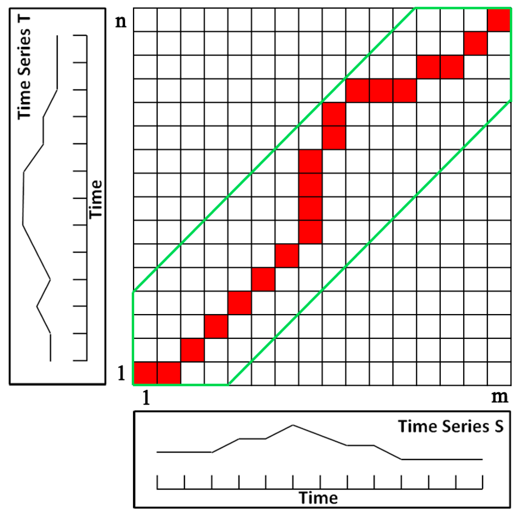
Figure 6.
The principle of MST segmentation.

Figure 7.
Flow chart of the STS classification method.
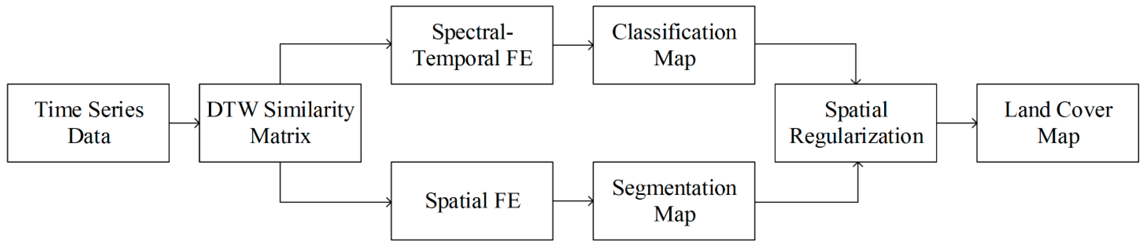
Figure 8.
Illinois classification results. Green = soybeans; yellow = corn; gray = developed/open space; pale green = grass/pasture; black = background (CDL classes covering ≤2% of the study area). (a) TI. (b) PCA. (c) LE-SAM-R. (d) LE-DTW. (e) STS.
Figure 8.
Illinois classification results. Green = soybeans; yellow = corn; gray = developed/open space; pale green = grass/pasture; black = background (CDL classes covering ≤2% of the study area). (a) TI. (b) PCA. (c) LE-SAM-R. (d) LE-DTW. (e) STS.
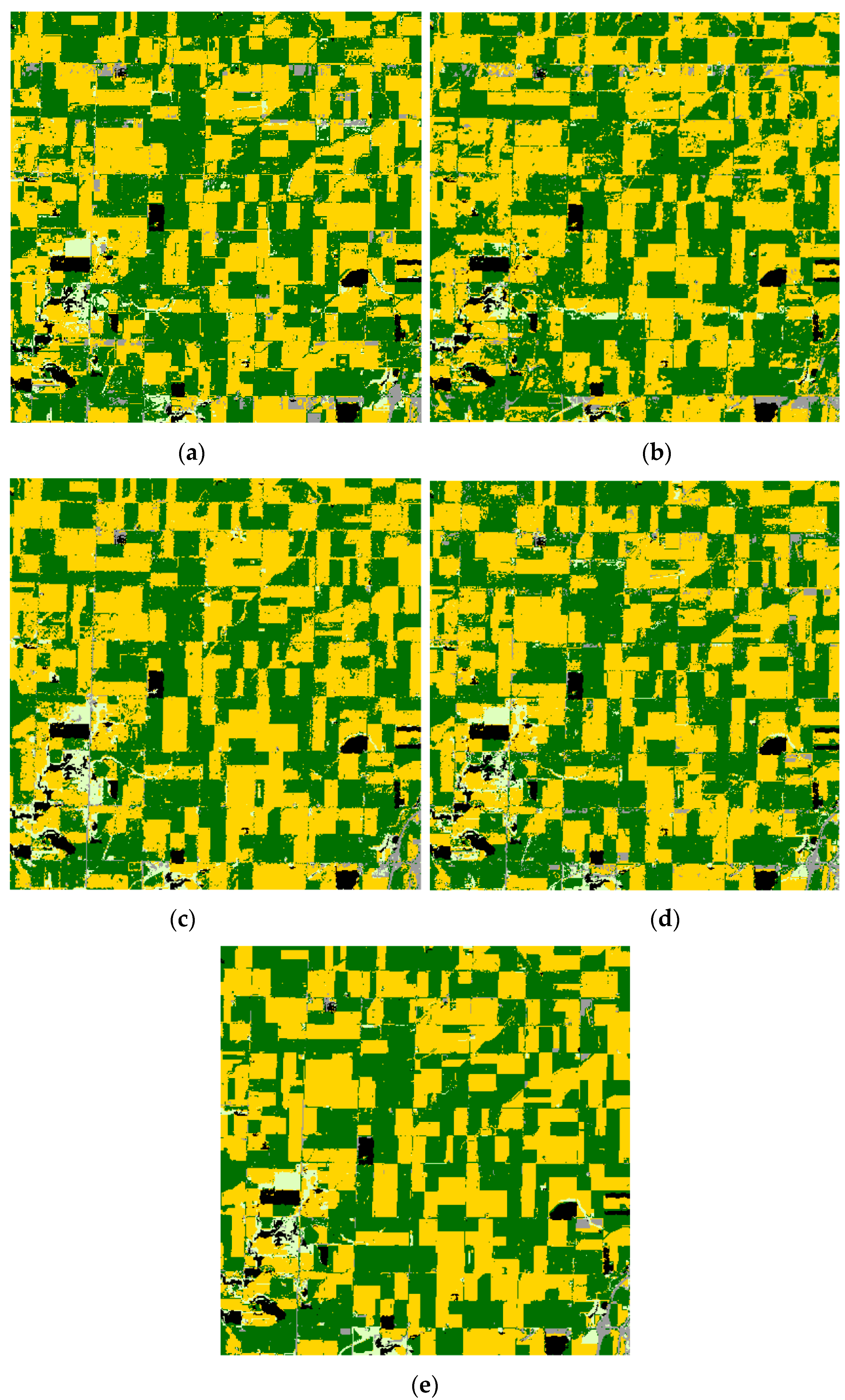
Figure 9.
South Dakota classification results. Green = soybeans; yellow = corn; gray = developed/open space; pale green = grass/pasture; magenta = alfalfa; black = background (CDL classes covering ≤2% of the study area). (a) TI. (b) PCA. (c) LE-SAM-R. (d) LE-DTW. (e) STS.
Figure 9.
South Dakota classification results. Green = soybeans; yellow = corn; gray = developed/open space; pale green = grass/pasture; magenta = alfalfa; black = background (CDL classes covering ≤2% of the study area). (a) TI. (b) PCA. (c) LE-SAM-R. (d) LE-DTW. (e) STS.


Figure 10.
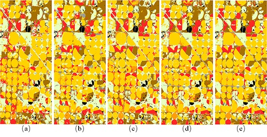
Texas classification results. Yellow = corn; brown = winter wheat; gray = developed/open space; pale green = grass/pasture; orange = sorghum; red = cotton; black = background (CDL classes covering ≤2% of the study area). (a) TI. (b) PCA. (c) LE-SAM-R. (d) LE-DTW. (e) STS.
Figure 10.
Texas classification results. Yellow = corn; brown = winter wheat; gray = developed/open space; pale green = grass/pasture; orange = sorghum; red = cotton; black = background (CDL classes covering ≤2% of the study area). (a) TI. (b) PCA. (c) LE-SAM-R. (d) LE-DTW. (e) STS.
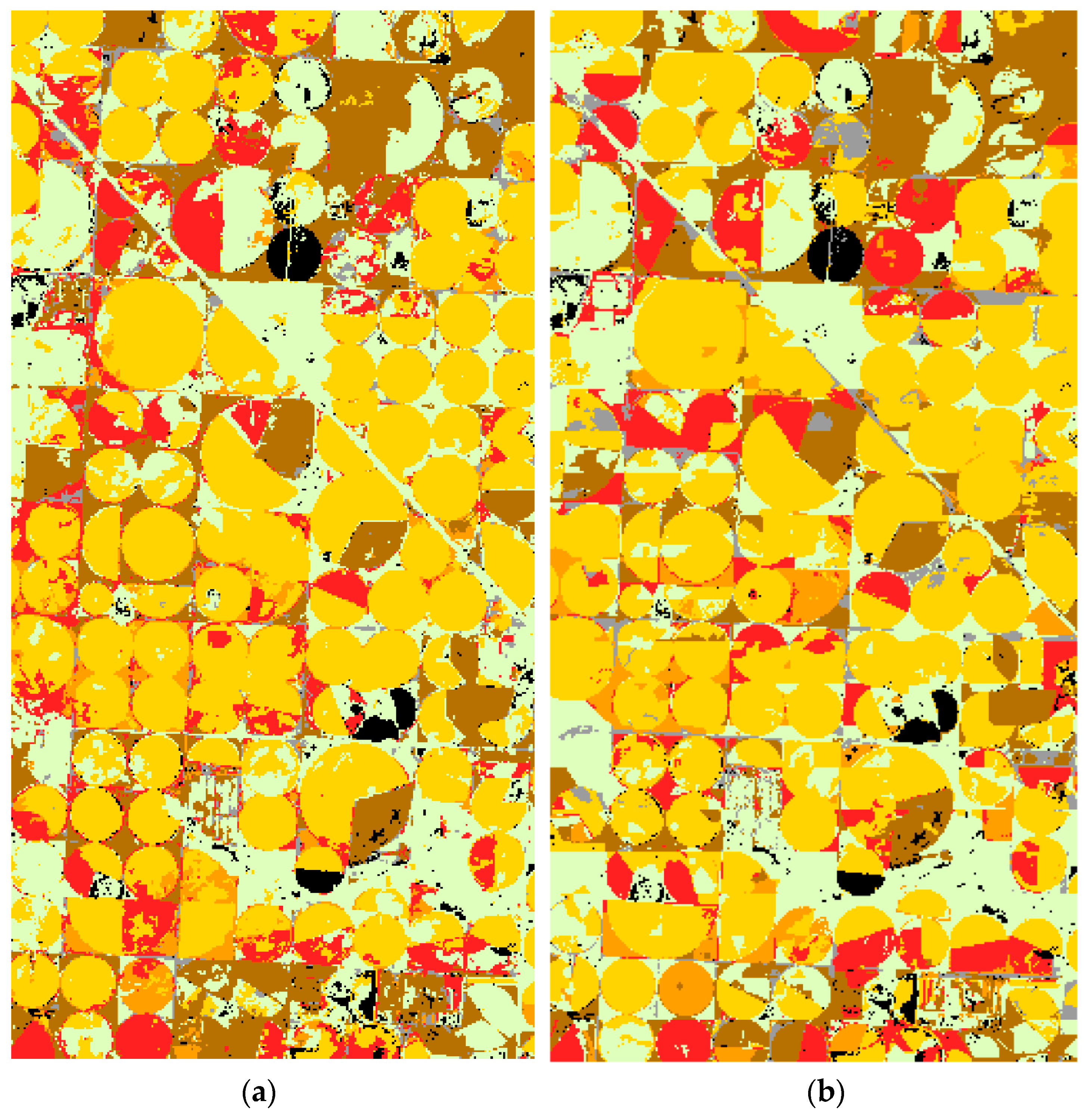

Figure 11.
Sensitivity to the different training data percentage (0.1%, 0.3%, 0.5%, 0.7%, 0.9%, 1%, 2%, 3%, 4%, 5%, 6%, 7%, 8%, 9% and 10%). At each percentage on three study areas, the mean overall accuracies of the LE-DTW (green) and STS (blue) calculated by 10 independent classifications are shown.


Table 1.
Comparison of five classification methods.
| Abbreviation | Classification Method |
|---|---|
| TI | Temporal interpolation + RF/SVM |
| PCA | Temporal interpolation + PCA + RF/SVM |
| LE-SAM-R | Temporal interpolation + LE-SAM + RF/SVM |
| LE-DTW | LE-DTW + RF/SVM |
| STS | LE-DTW + RF/SVM + MST-DTW |
Table 2.
The overall accuracies and kappa index of five classification methods.
| Classification Method | Illinois | South Dakota | Texas | ||||
|---|---|---|---|---|---|---|---|
| OA | Kappa | OA | Kappa | OA | Kappa | ||
| TI | SVM | 75.92% | 0.5801 | 83.47% | 0.7532 | 64.97% | 0.5173 |
| RF | 77.11% | 0.5997 | 85.40% | 0.7749 | 66.15% | 0.5285 | |
| PCA | SVM | 74.10% | 0.5388 | 78.86% | 0.6751 | 67.16% | 0.5495 |
| RF | 73.50% | 0.5683 | 80.39% | 0.7608 | 65.99% | 0.5610 | |
| LE-SAM-R | SVM | 78.64% | 0.6234 | 84.50% | 0.7641 | 70.67% | 0.5987 |
| RF | 80.74% | 0.6629 | 86.64% | 0.7982 | 73.33% | 0.6379 | |
| LE-DTW | SVM | 80.92% | 0.6649 | 86.72% | 0.7986 | 73.37% | 0.6383 |
| RF | 80.75% | 0.6655 | 87.17% | 0.8074 | 76.59% | 0.6829 | |
| STS | SVM | 82.92% | 0.7009 | 90.66% | 0.8589 | 78.35% | 0.7072 |
| RF | 82.41% | 0.6913 | 91.18% | 0.8668 | 77.72% | 0.6965 | |
Table 3.
Mean producer and user accuracies of classification based on TI + RF method.
| Soybeans | Corn | Developed/Open Space | Grass/Pasture | ||||
| Illinois | Producer’s accuracy | 81.18% | 79.31% | 6.74% | 16.11% | ||
| User’s accuracy | 83.81% | 85.20% | 1.89% | 13.01% | |||
| Soybeans | Corn | Developed/Open Space | Grass/Pasture | Alfalfa | |||
| South Dakota | Producer’s accuracy | 87.98% | 84.48% | 37.53% | 44.63% | 87.55% | |
| User’s accuracy | 88.05% | 87.40% | 9.36% | 8.43% | 88.01% | ||
| Winter Wheat | Corn | Developed/Open Space | Grass/Pasture | Sorghum | Cotton | ||
| Texas | Producer’s accuracy | 58.26% | 76.47% | 27.98% | 61.74% | 30.52% | 49.46% |
| User’s accuracy | 68.27% | 89.91% | 2.75% | 59.20% | 20.98% | 28.98% | |
Table 4.
Mean producer and user accuracies of classification based on LE-DTW+RF method.
| Soybeans | Corn | Developed/Open Space | Grass/Pasture | ||||
| Illinois | Producer’s accuracy | 81.79% | 84.12% | 48.15% | 54.29% | ||
| User’s accuracy | 87.53% | 85.58% | 15.31% | 38.72% | |||
| Soybeans | Corn | Developed/Open Space | Grass/Pasture | Alfalfa | |||
| South Dakota | Producer’s accuracy | 91.88% | 88.42% | 46.61% | 40.22% | 91.52% | |
| User’s accuracy | 90.73% | 92.23% | 37.03% | 35.95% | 92.61% | ||
| Winter Wheat | Corn | Developed/Open Space | Grass/Pasture | Sorghum | Cotton | ||
| Texas | Producer’s accuracy | 75.81% | 85.07% | 44.20% | 70.80% | 62.48% | 73.76% |
| User’s accuracy | 76.35% | 90.49% | 27.68% | 73.13% | 52.42% | 70.14% | |
Table 5.
Mean producer and user accuracies of classification based on PCA + RF method.
| Soybeans | Corn | Developed/Open Space | Grass/Pasture | ||||
| Illinois | Producer’s accuracy | 76.43% | 77.62% | 32.00% | 46.85% | ||
| User’s accuracy | 82.03% | 82.75% | 11.87% | 18.59% | |||
| Soybeans | Corn | Developed/Open Space | Grass/Pasture | Alfalfa | |||
| South Dakota | Producer’s accuracy | 86.02% | 87.16% | 47.24% | 44.13% | 86.44% | |
| User’s accuracy | 89.79% | 90.06% | 26.65% | 20.52% | 88.75% | ||
| Winter Wheat | Corn | Developed/Open Space | Grass/Pasture | Sorghum | Cotton | ||
| Texas | Producer’s accuracy | 69.30% | 80.96% | 24.53% | 58.97% | 41.56% | 54.77% |
| User’s accuracy | 68.16% | 84.34% | 11.26% | 64.01% | 32.25% | 50.65% | |
Table 6.
Mean producer and user accuracies of classification based on LE-SAM-R+RF method.
| Soybeans | Corn | Developed/Open Space | Grass/Pasture | ||||
| Illinois | Producer’s accuracy | 82.53% | 81.53% | 40.25% | 57.58% | ||
| User’s accuracy | 85.65% | 87.41% | 17.89% | 42.57% | |||
| Soybeans | Corn | Developed/Open Space | Grass/Pasture | Alfalfa | |||
| South Dakota | Producer’s accuracy | 88.01% | 88.87% | 56.30% | 47.83% | 91.11% | |
| User’s accuracy | 90.65% | 92.90% | 43.06% | 36.29% | 84.24% | ||
| Winter Wheat | Corn | Developed/Open Space | Grass/Pasture | Sorghum | Cotton | ||
| Texas | Producer’s accuracy | 72.20% | 84.44% | 31.10% | 64.62% | 52.11% | 67.15% |
| User’s accuracy | 76.32% | 90.42% | 9.42% | 65.31% | 44.76% | 69.58% | |
Table 7.
Mean producer and user accuracies of classification based on STS (using RF classifier) method.
Table 7.
Mean producer and user accuracies of classification based on STS (using RF classifier) method.
| Soybeans | Corn | Developed/Open Space | Grass/Pasture | ||||
| Illinois | Producer’s accuracy | 82.61% | 84.99% | 56.88% | 59.03% | ||
| User’s accuracy | 89.65% | 87.92% | 21.19% | 38.23% | |||
| Soybeans | Corn | Developed/Open Space | Grass/Pasture | Alfalfa | |||
| South Dakota | Producer’s accuracy | 92.72% | 92.36% | 65.70% | 56.15% | 94.95% | |
| User’s accuracy | 95.46% | 96.03% | 46.86% | 36.76% | 93.25% | ||
| Winter Wheat | Corn | Developed/Open Space | Grass/Pasture | Sorghum | Cotton | ||
| Texas | Producer’s accuracy | 75.82% | 84.06% | 46.31% | 74.06% | 64.88% | 75.97% |
| User’s accuracy | 78.84% | 93.84% | 25.86% | 71.13% | 52.87% | 69.63% | |
© 2018 by the authors. Licensee MDPI, Basel, Switzerland. This article is an open access article distributed under the terms and conditions of the Creative Commons Attribution (CC BY) license (http://creativecommons.org/licenses/by/4.0/).
Share and Cite
MDPI and ACS Style
Zhai, Y.; Qu, Z.; Hao, L. Land Cover Classification Using Integrated Spectral, Temporal, and Spatial Features Derived from Remotely Sensed Images. Remote Sens. 2018, 10, 383. https://doi.org/10.3390/rs10030383
AMA Style
Zhai Y, Qu Z, Hao L. Land Cover Classification Using Integrated Spectral, Temporal, and Spatial Features Derived from Remotely Sensed Images. Remote Sensing. 2018; 10(3):383. https://doi.org/10.3390/rs10030383
Chicago/Turabian StyleZhai, Yongguang, Zhongyi Qu, and Lei Hao. 2018. "Land Cover Classification Using Integrated Spectral, Temporal, and Spatial Features Derived from Remotely Sensed Images" Remote Sensing 10, no. 3: 383. https://doi.org/10.3390/rs10030383
Note that from the first issue of 2016, this journal uses article numbers instead of page numbers. See further details here.