Evaluating Endmember and Band Selection Techniques for Multiple Endmember Spectral Mixture Analysis using Post-Fire Imaging Spectroscopy

 , ,
, ,
Abstract
:
1. Introduction
2. Methodology
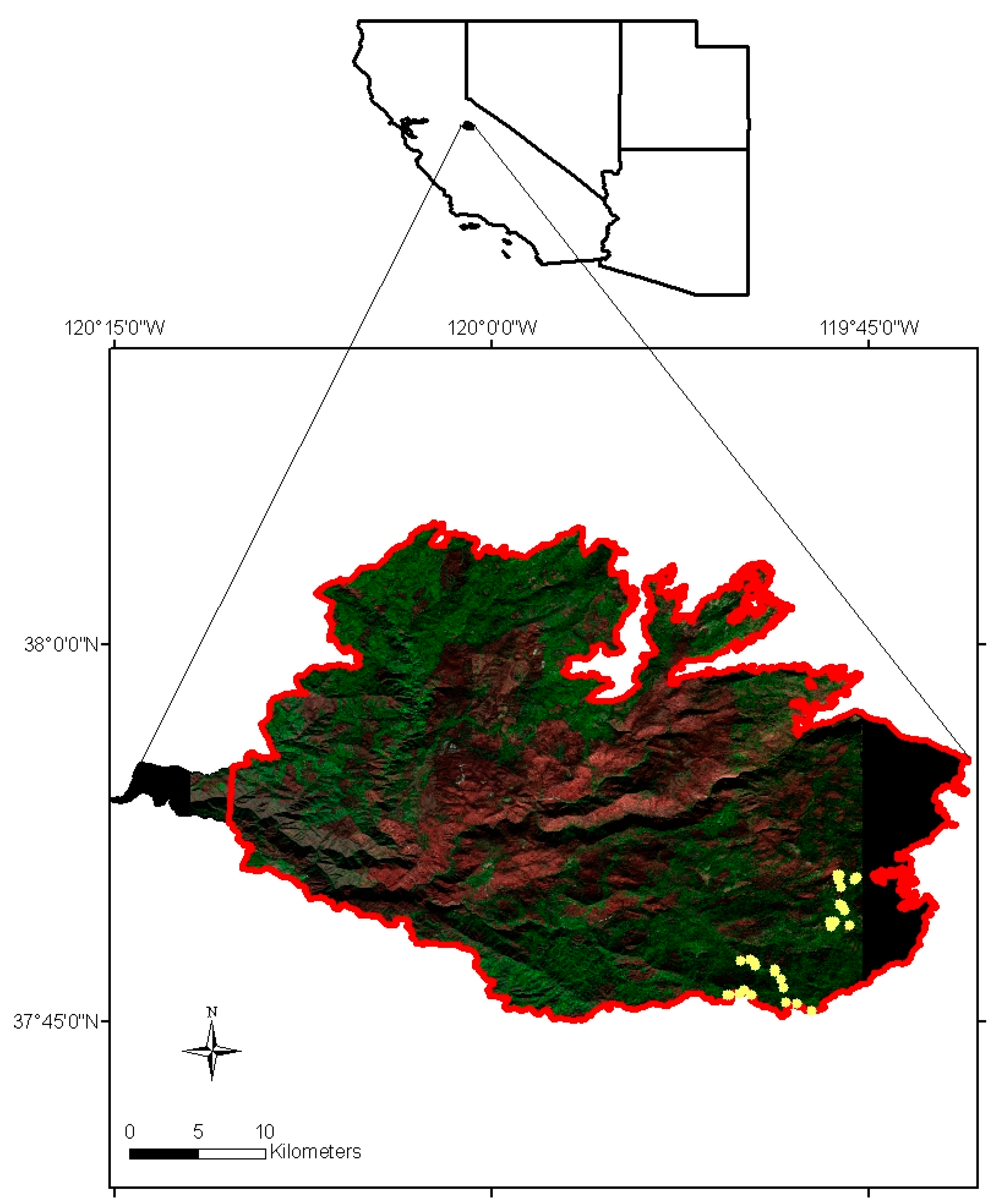
2.1. Study Area
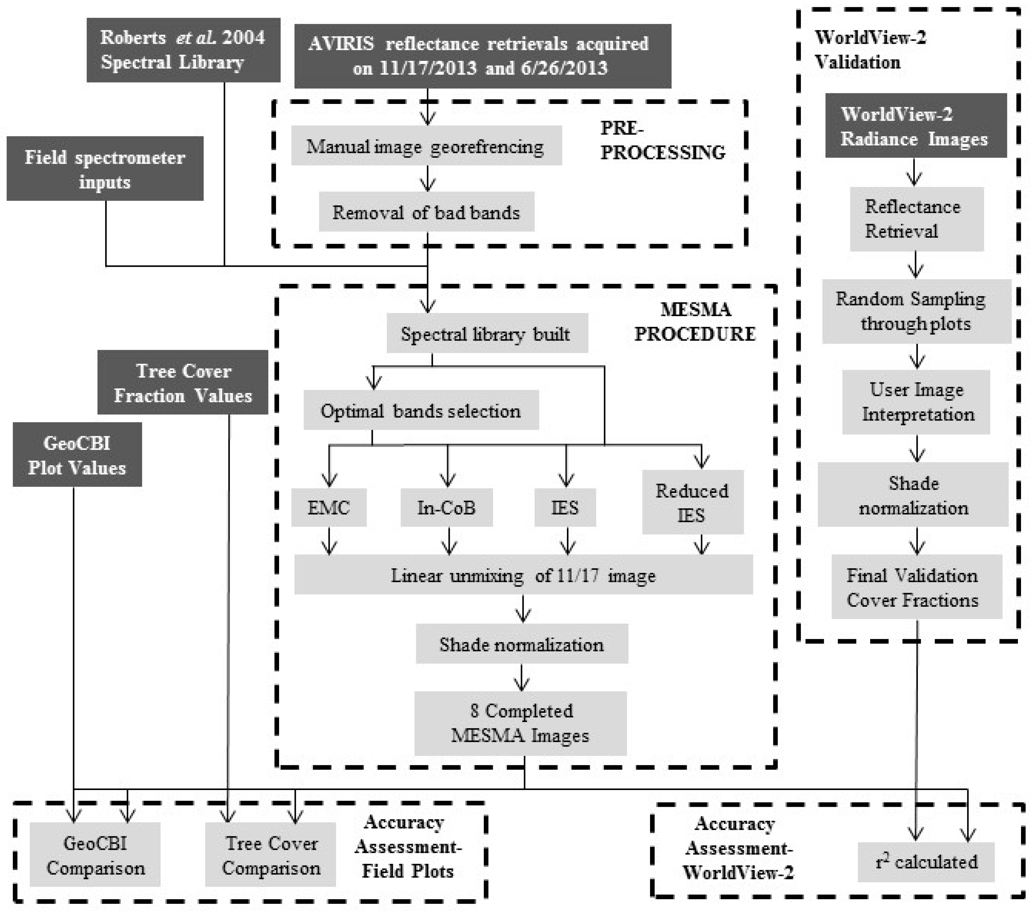
2.2. AVIRIS Imagery and MESMA
2.2.1. Preprocessing
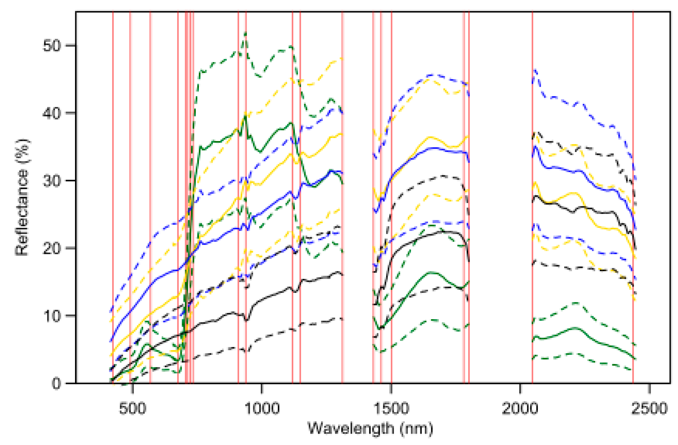
2.2.2. Spectral Library
2.2.3. Band Selection
2.2.4. Endmember Selection
2.2.5. MESMA
2.3. Validation
2.3.1. WorldView-2 Imagery
2.3.2. Field Plots
3. Results
3.1. uSZU Band Selection
3.2. Endmember Selection and Processing Times
3.3. Unmixed Images and Overall Model Comparison
3.4. Endmember Sources in Model Selection and the Image
3.5. Validation
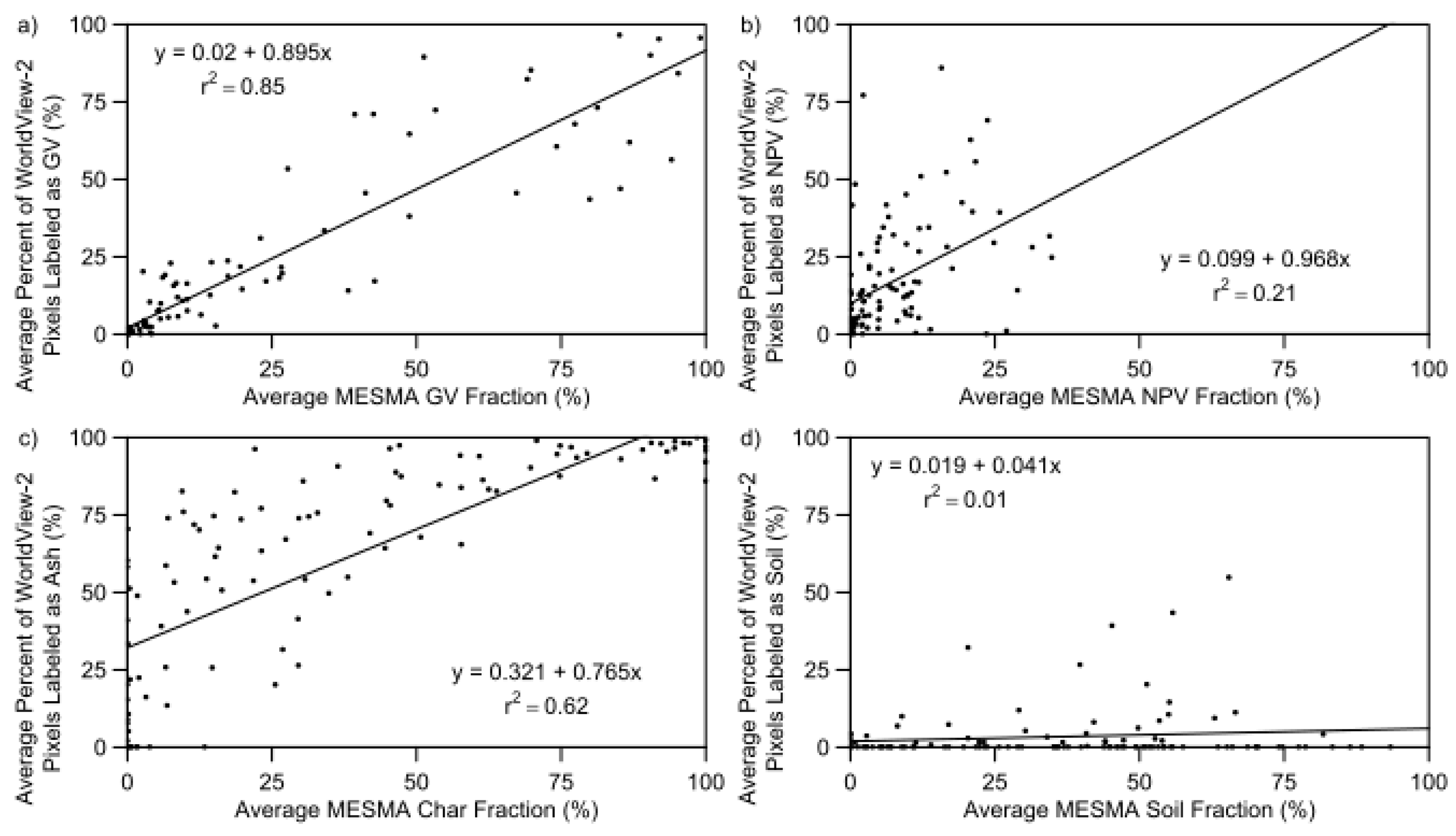
3.5.1. WorldView-2 Based Validation
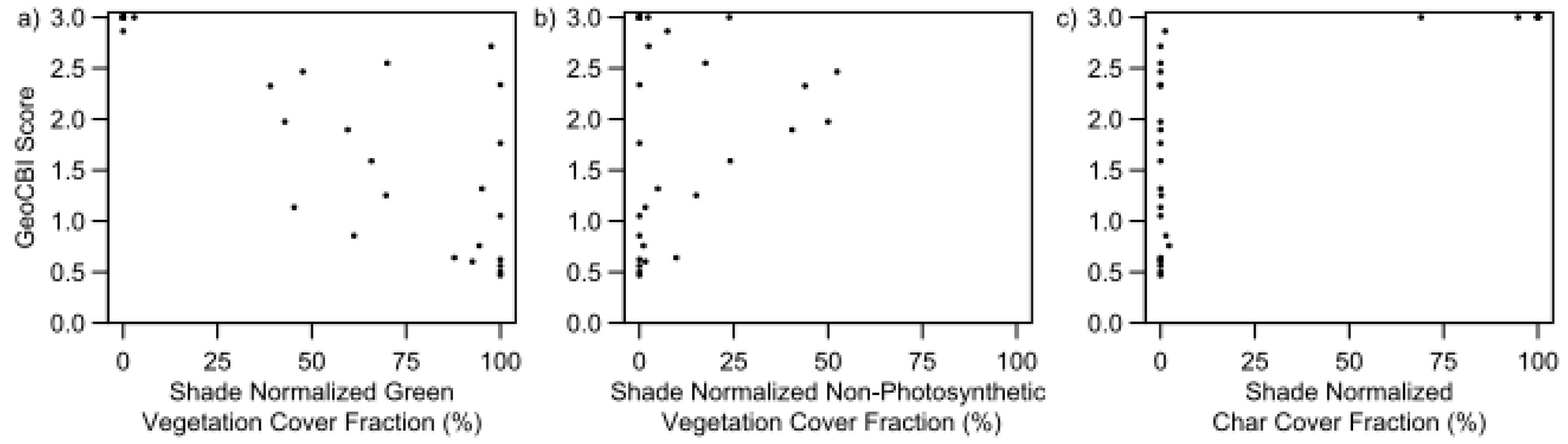
3.5.2. Comparison with GeoCBI Plot Data
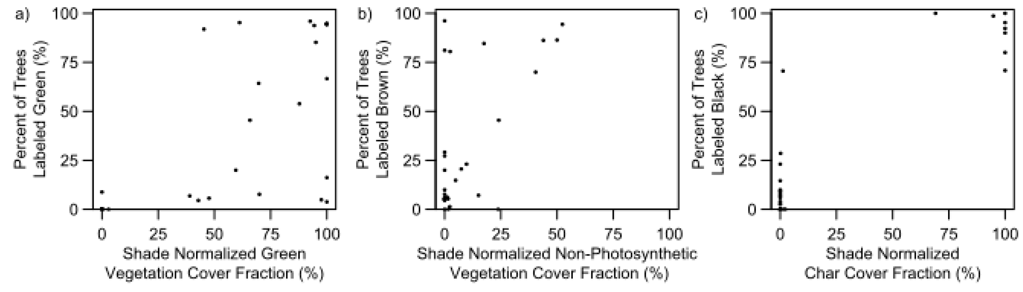
3.5.3. Comparison with Field Tree Status Data
4. Discussion
4.1. Potential Bias and Uncertainty in the Cover Types
4.2. Evaluation of MESMA Techniques’ Performance
4.3. Endmember Sources and Endmember Selection
4.4. SMA as a Novel Means for Assessing Fire Severity
5. Conclusions
Acknowledgments
Author Contributions
Conflicts of Interest
References
- Dennison, P.E.; Brewer, S.C.; Arnold, J.D.; Moritz, M.A. Large Wildfire Trend in the Western United States, 1984–2011. Geophys. Res. Lett. 2014, 41, 2928–2933. [Google Scholar] [CrossRef]
- Miller, J.D.; Safford, H.D.; Crimmins, M.; Thode, A.E. Quantitative evidence for increasing forest fire severity in the Sierra Nevada and southern Cascade Mountains, California and Nevada, USA. Ecosystems 2009, 12, 16–32. [Google Scholar] [CrossRef]
- Steel, Z.L.; Safford, H.D.; Viers, J.H. The fire frequency-severity relationship and the legacy of fire suppression in California forests. Ecosphere 2015, 6, 8. [Google Scholar] [CrossRef]
- Key, C.H.; Benson, N.C. Landscape Assessment: Sampling and Analysis Methods; General Technical Report RMRS-GTR-164-CD; USDA Forest Service: Fort Collins, CO, USA, 2006; pp. 1–55. [Google Scholar]
- Miller, J.D.; Thode, A.E. Quantifying burn severity in a heterogeneous landscape with a relative version of the delta Normalized Burn Ratio (dNBR). Remote Sens. Environ. 2007, 109, 66–80. [Google Scholar] [CrossRef]
- Cocke, A.E.; Fulé, P.Z.; Crouse, J.E. Comparison of burn severity assessments using Differenced Normalized Burn Ratio and ground data. Int. J. Wildl. Fire 2005, 14, 189. [Google Scholar] [CrossRef]
- Van Wagtendonk, J.W.; Root, R.R.; Key, C.H. Comparison of AVIRIS and Landsat ETM+ detection capabilities for burn severity. Remote Sens. Environ. 2004, 92, 397–408. [Google Scholar] [CrossRef]
- Smith, A.M.S.; Eitel, J.U.H.; Hudak, A.T. Spectral analysis of charcoal on soils: Implications for wildland fire severity mapping methods. Int. J. Wildl. Fire 2010, 19, 976–983. [Google Scholar] [CrossRef]
- Epting, J.; Verbyla, D.; Sorbel, B. Evaluation of remotely sensed indices for assessing burn severity in interior Alaska using Landsat TM and ETM+. Remote Sens. Environ. 2005, 96, 328–339. [Google Scholar] [CrossRef]
- Lentile, L.B.; Smith, A.M.S.; Hudak, A.T.; Morgan, P.; Bobbitt, M.J.; Lewis, S.A.; Robichaud, P.R. Remote sensing for prediction of 1-year post-fire ecosystem condition. Int. J. Wildl. Fire 2009, 18, 594–608. [Google Scholar] [CrossRef]
- Adams, J.B.; Smith, M.O.; Johnson, P.E. Spectral mixture modeling: A new analysis of rock and soil types at the Viking Lander 1 Site. J. Geophys. Res. Solid Earth 1986, 91, 8098–8112. [Google Scholar] [CrossRef]
- Roberts, D.A.; Smith, M.O.; Adams, J.B. Green vegetation, nonphotosynthetic vegetation, and soils in AVIRIS data. Remote Sens. Environ. 1993, 44, 255–269. [Google Scholar] [CrossRef]
- Rogan, J.; Franklin, J. Mapping Wildfire Burn Severity in Southern California Forests and Shrublands Using Enhanced Thematic Mapper Imagery. Geocarto Int. 2001, 16, 91–106. [Google Scholar] [CrossRef]
- Quintano, C.; Fernández-Manso, A.; Roberts, D.A. Multiple Endmember Spectral Mixture Analysis (MESMA) to map burn severity levels from Landsat images in Mediterranean countries. Remote Sens. Environ. 2013, 136, 76–88. [Google Scholar] [CrossRef]
- Hudak, A.T.; Morgan, P.; Bobbitt, M.J.; Smith, A.M.S.; Lewis, S.A.; Lentile, L.B.; Robichaud, P.R.; Clark, J.T.; Mckinley, R.A. The Relationship of Multispectral Satellite Imagery. Fire Ecol. 2007, 3, 64–90. [Google Scholar] [CrossRef]
- Kokaly, R.F.; Rockwell, B.W.; Haire, S.L.; King, T.V.V. Characterization of post-fire surface cover, soils, and burn severity at the Cerro Grande Fire, New Mexico, using hyperspectral and multispectral remote sensing. Remote Sens. Environ. 2007, 106, 305–325. [Google Scholar] [CrossRef]
- Robichaud, P.R.; Lewis, S.A.; Laes, D.Y.M.; Hudak, A.T.; Kokaly, R.F.; Zamudio, J.A. Postfire soil burn severity mapping with hyperspectral image unmixing. Remote Sens. Environ. 2007, 108, 467–480. [Google Scholar] [CrossRef]
- Veraverbeke, S.; Hook, S. Evaluating spectral indices and spectral mixture analysis for assessing fire severity, combustion completeness and carbon emissions. Int. J. Wildl. Fire 2013, 22, 707–720. [Google Scholar] [CrossRef]
- Lentile, L.B.; Holden, Z.A.; Smith, A.M.S.; Falkowski, M.J.; Hudak, A.T.; Morgan, P.; Lewis, S.A.; Gessler, P.E.; Benson, N.C. Remote sensing techniques to assess active fire characteristics and post-fire effects. Int. J. Wildl. Fire 2006, 15, 319–345. [Google Scholar] [CrossRef]
- Veraverbeke, S.; Lhermitte, S.; Verstraeten, W.W.; Goossens, R. The temporal dimension of differenced Normalized Burn Ratio (dNBR) fire/burn severity studies: The case of the large 2007 Peloponnese wildfires in Greece. Remote Sens. Environ. 2010, 114, 2548–2563. [Google Scholar] [CrossRef] [Green Version]
- Roberts, D.A.; Gardner, M.; Church, R.; Ustin, S.L.; Scheer, G.; Green, R.O. Mapping chaparral in the Santa Monica Mountains using multiple endmember spectral mixture models. Remote Sens. Environ. 1998, 65, 267–279. [Google Scholar] [CrossRef]
- Somers, B.; Asner, G.P.; Tits, L.; Coppin, P. Endmember variability in Spectral Mixture Analysis: A review. Remote Sens. Environ. 2011, 115, 1603–1616. [Google Scholar] [CrossRef]
- Green, R.O.; Eastwood, M.L.; Sarture, C.M.; Chrien, T.G.; Aronsson, M.; Chippendale, B.J.; Faust, J.A.; Pavri, B.E.; Chovit, C.J.; Solis, M.; et al. Imaging spectroscopy and the Airborne Visible/Infrared Imaging Spectrometer (AVIRIS). Remote Sens. Environ. 1998, 65, 227–248. [Google Scholar] [CrossRef]
- Jia, G.J.; Burke, I.C.; Goetz, A.F.H.; Kaufmann, M.R.; Kindel, B.C. Assessing spatial patterns of forest fuel using AVIRIS data. Remote Sens. Environ. 2006, 102, 318–327. [Google Scholar] [CrossRef]
- Guanter, L.; Kaufmann, H.; Segl, K.; Foerster, S.; Rogass, C.; Chabrillat, S.; Kuester, T.; Hollstein, A.; Rossner, G.; Chlebek, C.; et al. The EnMAP spaceborne imaging spectroscopy mission for earth observation. Remote Sens. 2015, 7, 8830–8857. [Google Scholar] [CrossRef] [Green Version]
- Stefano, P.; Angelo, P.; Simone, P.; Filomena, R.; Federico, S.; Tiziana, S.; Umberto, A.; Vincenzo, C.; Acito, N.; Marco, D.; et al. The PRISMA hyperspectral mission: Science activities and opportunities for agriculture and land monitoring. Int. Geosci. Remote Sens. Symp. 2013, 2567, 4558–4561. [Google Scholar]
- Lee, C.M.; Cable, M.L.; Hook, S.J.; Green, R.O.; Ustin, S.L.; Mandl, D.J.; Middleton, E.M. An introduction to the NASA Hyperspectral InfraRed Imager (HyspIRI) mission and preparatory activities. Remote Sens. Environ. 2015, 167, 6–19. [Google Scholar] [CrossRef]
- Boardman, J.; Kruse, F.; Green, R.O. Mapping Target Signatures via Partial Unmixing of AVIRIS Data. In Proceedings of the Fifth Annual JPL Airborne Earth Science Workshop, Volume 1: AVIRIS Workshop, Pasadena, CA, USA, 23–26 January 1995; pp. 23–26. [Google Scholar]
- Tompkins, S.; Mustard, J.F.; Pieters, C.M.; Forsyth, D.W. Optimization of endmembers for spectral mixture analysis. Remote Sens. Environ. 1997, 59, 472–489. [Google Scholar] [CrossRef]
- Dennison, P.E.; Roberts, D.A.; Thorgusen, S.R.; Regelbrugge, J.C.; Weise, D.; Lee, C. Modeling seasonal changes in live fuel moisture and equivalent water thickness using a cumulative water balance index. Remote Sens. Environ. 2003, 88, 442–452. [Google Scholar] [CrossRef]
- Schaaf, A.N.; Dennison, P.E.; Fryer, G.K.; Roth, K.L.; Roberts, D.A. Mapping Plant Functional Types at Multiple Spatial Resolutions Using Imaging Spectrometer Data. GISci. Remote Sens. 2011, 48, 324–344. [Google Scholar] [CrossRef]
- Roth, K.L.; Dennison, P.E.; Roberts, D.A. Comparing endmember selection techniques for accurate mapping of plant species and land cover using imaging spectrometer data. Remote Sens. Environ. 2012, 127, 139–152. [Google Scholar] [CrossRef]
- Dennison, P.E.; Roberts, D.A. Endmember selection for multiple endmember spectral mixture analysis using endmember average RMSE. Remote Sens. Environ. 2003, 87, 123–135. [Google Scholar] [CrossRef]
- Dennison, P.E.; Halligan, K.Q.; Roberts, D.A. A comparison of error metrics and constraints for multiple endmember spectral mixture analysis and spectral angle mapper. Remote Sens. Environ. 2004, 93, 359–367. [Google Scholar] [CrossRef]
- Roberts, D.A.; Quattrochi, D.A.; Hulley, G.C.; Hook, S.J.; Green, R.O. Synergies between VSWIR and TIR data for the urban environment: An evaluation of the potential for the Hyperspectral Infrared Imager (HyspIRI) Decadal Survey mission. Remote Sens. Environ. 2012, 117, 83–101. [Google Scholar] [CrossRef]
- Keshava, N.; Mustard, J.F. Spectral unmixing. IEEE Signal Process. Mag. 2002, 19, 44–57. [Google Scholar] [CrossRef]
- Veganzones, M.A.; Grana, M. Endmember Extraction Methods: A Short Review. In Proceedings of the International Conference on Knowledge-Based and Intelligent Information and Engineering Systems, Zagreb, Croatia, 3–5 September 2008; pp. 400–407. [Google Scholar]
- Parente, M.; Plaza, A. Survey of geometric and statistical unmixing algorithms for hyperspectral images. In Proceedings of the 2010 2nd Workshop on Hyperspectral Image and Signal Processing: Evolution in Remote Sensing (WHISPERS), Reykjavik, Iceland, 14–16 June 2010. [Google Scholar]
- Pal, M.; Foody, G.M. Feature Selection for Classification of Hyperspectral Data by SVM. IEEE Trans. Geosci. Remote Sens. 2010, 48, 2297–2307. [Google Scholar] [CrossRef]
- Miao, X.; Gong, P.; Swope, S.; Pu, R.; Carruthers, R.; Anderson, G.L.; Heaton, J.S.; Tracy, C.R. Estimation of yellow starthistle abundance through CASI-2 hyperspectral imagery using linear spectral mixture models. Remote Sens. Environ. 2006, 101, 329–341. [Google Scholar] [CrossRef]
- Green, A.A.; Berman, M.; Switzer, P.; Craig, M.D. A Transformation for Ordering Multispectral Data in Terms of Image Quality with Implications for Noise Removal. IEEE Trans. Geosci. Remote Sens. 1988, 26, 65–74. [Google Scholar] [CrossRef]
- Li, J. Wavelet-based feature extraction for improved endmember abundance estimation in linear unmixing of hyperspectral signals. IEEE Trans. Geosci. Remote Sens. 2004, 42, 644–649. [Google Scholar] [CrossRef]
- Asner, G.P.; Lobell, D.B. A biogeophysical approach for automated SWIR unmixing of soils and vegetation. Remote Sens. Environ. 2000, 74, 99–112. [Google Scholar] [CrossRef]
- Somers, B.; Delalieux, S.; Verstraeten, W.W.; van Aardt, J.A.N.; Albrigo, G.L.; Coppin, P. An automated waveband selection technique for optimized hyperspectral mixture analysis. Int. J. Remote Sens. 2010, 31, 5549–5568. [Google Scholar] [CrossRef]
- Zhao, C.H.; Cui, S.L.; Qi, B. A sparse multiple endmember spectral mixture analysis algorithm of hyperspectral image. In Proceedings of the International Conference on Signal Processing, Hangzhou, China, 19–23 October 2014; pp. 687–692. [Google Scholar]
- Peterson, S.H.; Roberts, D.A.; Beland, M.; Kokaly, R.F.; Ustin, S.L. Oil detection in the coastal marshes of Louisiana using MESMA applied to band subsets of AVIRIS data. Remote Sens. Environ. 2015, 159, 222–231. [Google Scholar] [CrossRef]
- Somers, B.; Asner, G.P. Multi-temporal hyperspectral mixture analysis and feature selection for invasive species mapping in rainforests. Remote Sens. Environ. 2013, 136, 14–27. [Google Scholar] [CrossRef]
- Thompson, D.R.; Gao, B.C.; Green, R.O.; Roberts, D.A.; Dennison, P.E.; Lundeen, S.R. Atmospheric correction for global mapping spectroscopy: ATREM advances for the HyspIRI preparatory campaign. Remote Sens. Environ. 2015, 167, 64–77. [Google Scholar] [CrossRef]
- Settle, J.; Campbell, N. On the errors of two estimators of sub-pixel fractional cover when mixing is linear. IEEE Trans. Geosci. Remote Sens. 1998, 36, 163–170. [Google Scholar] [CrossRef]
- Baldridge, A.M.; Hook, S.J.; Crowley, J.K.; Marion, G.M.; Kargel, J.S.; Michalski, J.L.; Thomson, B.J.; De Souza Filho, C.R.; Bridges, N.T.; Brown, A.J. Contemporaneous deposition of phyllosilicates and sulfates: Using Australian acidic saline lake deposits to describe geochemical variability on Mars. Geophys. Res. Lett. 2009, 36, 1–6. [Google Scholar] [CrossRef]
- Roberts, D.A.; Ustin, S.L.; Ogunjemiyo, S.; Greenberg, J.; Dobrowski, S.Z.; Chen, J.; Hinckley, T.M. Spectral and Structural Measures of Northwest Forest Vegetation at Leaf to Landscape Scales. Ecosystems 2004, 7, 545–562. [Google Scholar] [CrossRef]
- Roberts, D.A.; Dennison, P.E.; Gardner, M.E.; Hetzel, Y.; Ustin, S.L.; Lee, C.T. Evaluation of the potential of Hyperion for fire danger assessment by comparison to the airborne visible/infrared imaging spectrometer. IEEE Trans. Geosci. Remote Sens. 2003, 41, 1297–1310. [Google Scholar] [CrossRef]
- Kruse, F.; Lefkoff, A.B.; Boardman, J.W.; Heidebrecht, K.B.; Shapiro, A.T.; Barloon, P.J.; Goetz, A.F.H. The spectral image processing system (SIPS)—Interactive visualization and analysis of imaging spectrometer data. Remote Sens. Environ. 1993, 44, 145–163. [Google Scholar] [CrossRef]
- Cohen, J. A Coefficent of Agreement for Nominal Scales. Educ. Psychol. Meas. 1960, 20, 37–46. [Google Scholar]
- Roberts, D.A.; Alonzo, M.; Wetherley, E.B.; Dudley, K.L.; Dennison, P.E. Multiscale Analysis of Urban Areas Using Mixing Models. In Integrating Scale in Remote Sensing and GIS; CRC Press: Boca Raton, FL, USA, 2017; pp. 247–282. ISBN 9781315373720. [Google Scholar]
- Adams, J.B.; Gillespie, A.R. Remote Sensing of Landscapes with Spectral Images: A Physical Modeling Approach; Cambridge University Press: Cambridge, UK, 2006; ISBN 0521662214. [Google Scholar]
- De Santis, A.; Chuvieco, E. GeoCBI: A modified version of the Composite Burn Index for the initial assessment of the short-term burn severity from remotely sensed data. Remote Sens. Environ. 2009, 113, 554–562. [Google Scholar] [CrossRef]
- Veraverbeke, S.; Stavros, E.N.; Hook, S.J. Remote Sensing of Environment Assessing fire severity using imaging spectroscopy data from the Airborne Visible/Infrared Imaging Spectrometer (AVIRIS) and comparison with multispectral capabilities. Remote Sens. Environ. 2014, 154, 153–163. [Google Scholar] [CrossRef]
- Peterson, D.A.; Hyer, E.J.; Campbell, J.R.; Fromm, M.D.; Hair, J.W.; Butler, C.F.; Fenn, M.A. The 2013 Rim Fire: Implications for predicting extreme fire spread, pyroconvection, smoke emissions. Bull. Am. Meteorol. Soc. 2015, 96, 229–247. [Google Scholar] [CrossRef]
- Daughtry, C.S.T. Discriminating Crop Residues from Soil by Shortwave Infrared Reflectance. Agron. J. 2001, 93, 125–131. [Google Scholar] [CrossRef]
- Dudley, K.L.; Dennison, P.E.; Roth, K.L.; Roberts, D.A.; Coates, A.R. A multi-temporal spectral library approach for mapping vegetation species across spatial and temporal phenological gradients. Remote Sens. Environ. 2015, 167, 121–134. [Google Scholar] [CrossRef]
- Franke, J.; Roberts, D.A.; Halligan, K.; Menz, G. Hierarchical Multiple Endmember Spectral Mixture Analysis (MESMA) of hyperspectral imagery for urban environments. Remote Sens. Environ. 2009, 113, 1712–1723. [Google Scholar] [CrossRef]
- Herold, M.; Gardner, M.E.; Roberts, D. Spectral resolution requirements for mapping urban areas. IEEE Trans. Geosci. Remote Sens. 2003, 41, 1907–1919. [Google Scholar] [CrossRef]
- Hamlin, L.; Green, R.O.; Mouroulis, P.; Eastwood, M.; Wilson, D.; Dudik, M.; Paine, C. Imaging Spectrometer Science Measurements for Terrestrial Ecology: AVIRIS and New Developments. In Proceedings of the 2011 IEEE Aerospace Conference, Big Sky, MT, USA, 5–12 March 2011; pp. 1–8. [Google Scholar]
- Cansler, C.A.; McKenzie, D. How robust are burn severity indices when applied in a new region? Evaluation of alternate field-based and remote-sensing methods. Remote Sens. 2012, 4, 456–483. [Google Scholar] [CrossRef]
- Morgan, P.; Keane, R.E.; Dillon, G.K.; Jain, T.B.; Hudak, A.T.; Karau, E.C.; Sikkink, P.G.; Holden, Z.A.; Strand, E.K. Challenges of assessing fire and burn severity using field measures, remote sensing and modelling. Int. J. Wildl. Fire 2014, 23, 1045–1060. [Google Scholar] [CrossRef]


| Char | GV | NPV | Soil | Total | |
|---|---|---|---|---|---|
| 17 November AVIRIS | 457 | 308 | 0 | 358 | 1227 |
| 26 July AVIRIS | 0 | 1739 | 245 | 510 | 2634 |
| ASD | 21 | 0 | 3 | 46 | 70 |
| Wind River | 0 | 498 | 129 | 139 | 766 |
| Total | 478 | 2545 | 377 | 1053 | 4453 |
| Class | EMC | uSZU EMC | In-CoB | uSZU In-CoB | IES | uSZU IES | Reduced IES | uSZU Reduced IES |
|---|---|---|---|---|---|---|---|---|
| Char | 2 | 3 | 5 | 5 | 10 | 10 | 5 | 7 |
| GV | 2 | 2 | 14 | 17 | 31 | 42 | 25 | 40 |
| NPV | 3 | 2 | 11 | 11 | 36 | 40 | 32 | 37 |
| Soil | 2 | 2 | 15 | 16 | 55 | 53 | 35 | 38 |
| Total Models | 83 | 83 | 5729 | 7071 | 115,543 | 156,821 | 45,327 | 92,415 |
| Processing Time | 0.98 | 0.44 | 14.88 | 8.70 | 151.85 | 66.76 | 78.36 | 54.45 |
| EMC | uSZU EMC | In-CoB | uSZU In-CoB | IES | uSZU IES | Reduced IES | uSZU Reduced IES | |
|---|---|---|---|---|---|---|---|---|
| Modeled | 87.0% | 81.7% | 83.2% | 79.1% | 93.0% | 92.0% | 85.7% | 86.4% |
| Char | 36.9% | 53.1% | 47.3% | 36.9% | 33.4% | 42.9% | 41.6% | 34.4% |
| GV | 54.1% | 52.9% | 43.1% | 39.9% | 35.3% | 39.4% | 36.8% | 38.1% |
| NPV | 38.8% | 21.9% | 27.7% | 22.0% | 23.5% | 21.2% | 30.0% | 21.65 |
| Soil | 7.9% | 7.5% | 11.5% | 26.2% | 41.8% | 28.6% | 17.5% | 28.4% |
| Spectra Source | EMC | uSZU EMC | In-CoB | uSZU In-CoB | IES | uSZU IES | Reduced IES | uSZU Reduced IES |
|---|---|---|---|---|---|---|---|---|
| AVIRIS | 9 | 9 | 15 | 18 | 41 | 45 | 20 | 30 |
| ASD | 0 | 0 | 5 | 4 | 12 | 14 | 9 | 12 |
| Wind River | 0 | 0 | 25 | 27 | 79 | 86 | 68 | 80 |
| Spectra Source | EMC | uSZU EMC | In-CoB | uSZU In-CoB | IES | uSZU IES | Reduced IES | uSZU Reduced IES |
|---|---|---|---|---|---|---|---|---|
| Not Modeled | 13% | 18.3% | 16.8% | 20.9% | 7% | 8% | 14.3% | 13.6% |
| AVIRIS | 87% | 81.7% | 42.1% | 53.2% | 61.8% | 55.3% | 48.6% | 32.5% |
| ASD | 0 | 0 | 15.7% | 6.2% | 5.4% | 10.3% | 6.9% | 26.4% |
| Wind River | 0 | 0 | 45.8% | 38% | 47.1% | 44.4% | 47.6% | 41.6% |
| EMC | uSZU EMC | In-CoB | uSZU In-CoB | IES | uSZU IES | Reduced IES | uSZU Reduced IES | ||
|---|---|---|---|---|---|---|---|---|---|
| Char | r2 | 0.605 | 0.741 | 0.727 | 0.642 | 0.620 | 0.538 | 0.687 | 0.594 |
| Intercept | 0.355 | 0.303 | 0.212 | 0.202 | 0.321 | 0.223 | 0.255 | 0.310 | |
| Slope | 0.721 | 0.755 | 0.841 | 0.835 | 0.765 | 0.783 | 0.771 | 0.750 | |
| GV | r2 | 0.750 | 0.770 | 0.836 | 0.871 | 0.848 | 0.846 | 0.853 | 0.861 |
| Intercept | −0.054 | −0.023 | −0.026 | −0.065 | 0.020 | 0.000 | -0.010 | −0.019 | |
| Slope | 0.653 | 0.769 | 0.708 | 0.675 | 0.895 | 0.812 | 0.804 | 0.748 | |
| NPV | r2 | 0.086 | 0.099 | 0.164 | 0.249 | 0.209 | 0.237 | 0.165 | 0.245 |
| Intercept | 0.110 | 0.103 | 0.109 | 0.126 | 0.099 | 0.107 | 0.099 | 0.094 | |
| Slope | 0.240 | 0.521 | 0.426 | 0.375 | 0.968 | 0.943 | 0.377 | 0.699 | |
| Soil | r2 | 0.273 | 0.261 | 0.088 | 0.042 | 0.014 | 0.049 | 0.075 | 0.057 |
| Intercept | 0.013 | 0.015 | 0.015 | 0.013 | 0.019 | 0.016 | 0.011 | 0.012 | |
| Slope | 0.641 | 0.102 | 0.222 | 0.965 | 0.041 | 0.088 | 0.2 | 0.103 |
© 2018 by the authors. Licensee MDPI, Basel, Switzerland. This article is an open access article distributed under the terms and conditions of the Creative Commons Attribution (CC BY) license (http://creativecommons.org/licenses/by/4.0/).
Share and Cite
Tane, Z.; Roberts, D.; Veraverbeke, S.; Casas, Á.; Ramirez, C.; Ustin, S. Evaluating Endmember and Band Selection Techniques for Multiple Endmember Spectral Mixture Analysis using Post-Fire Imaging Spectroscopy. Remote Sens. 2018, 10, 389. https://doi.org/10.3390/rs10030389
Tane Z, Roberts D, Veraverbeke S, Casas Á, Ramirez C, Ustin S. Evaluating Endmember and Band Selection Techniques for Multiple Endmember Spectral Mixture Analysis using Post-Fire Imaging Spectroscopy. Remote Sensing. 2018; 10(3):389. https://doi.org/10.3390/rs10030389
Chicago/Turabian StyleTane, Zachary, Dar Roberts, Sander Veraverbeke, Ángeles Casas, Carlos Ramirez, and Susan Ustin. 2018. "Evaluating Endmember and Band Selection Techniques for Multiple Endmember Spectral Mixture Analysis using Post-Fire Imaging Spectroscopy" Remote Sensing 10, no. 3: 389. https://doi.org/10.3390/rs10030389