Article

Hydrological Variability and Changes in the Arctic Circumpolar Tundra and the Three Largest Pan-Arctic River Basins from 2002 to 2016

1
Japan Agency for Marine-Earth Science and Technology (JAMSTEC), 3173-25 Showamachi, Kanazawa-ku, Yokohama, Kanagawa 236-0001, Japan
2
Geospatial Information Authority of Japan, Kitasato 1-ban, Tsukuba, Ibaraki 305-0816, Japan
3
Institute of Industrial Science, The University of Tokyo, 4-6-1 Komaba, Meguro-ku, Tokyo 153-8505, Japan
4
Center for Environmental Remote Sensing (CEReS), Chiba University, 1-33, Yayoi-cho, Inage-ku, Chiba 263-8522, Japan
5
Graduate School of Bioresources, Mie University, 1577 Kurima-Machiya-Cho, Tsu, Mie 514-8507, Japan
6
Laboratoire d’Etudes en Géophysique et Océanographie Spatiales (LEGOS), Université de Toulouse, IRD, CNES, CNRS, UPS, 31400 Toulouse, France
7
Institute for Space-Earth Environmental Research, Nagoya University, Furo-cho, Chikusa-ku, Nagoya, Aichi 464-8601, Japan
*
Author to whom correspondence should be addressed.
Remote Sens. 2018, 10(3), 402; https://doi.org/10.3390/rs10030402
Submission received: 24 November 2017 / Revised: 19 January 2018 / Accepted: 26 January 2018 / Published: 6 March 2018

Abstract

:
The Arctic freshwater budget is critical for understanding the climate in the northern regions. However, the hydrology of the Arctic circumpolar tundra region (ACTR) and the largest pan-Arctic rivers are still not well understood. In this paper, we analyze the spatiotemporal variations in the terrestrial water storage (TWS) of the ACTR and three of the largest pan-Arctic river basins (Lena, Mackenzie, Yukon). To do this, we utilize monthly Gravity Recovery and Climate Experiment (GRACE) data from 2002 to 2016. Together with global land reanalysis, and river runoff data, we identify declining TWS trends throughout the ACTR that we attribute largely to increasing evapotranspiration driven by increasing summer air temperatures. In terms of regional changes, large and significant negative trends in TWS are observed mainly over the North American continent. At basin scale, we show that, in the Lena River basin, the autumnal TWS signal persists until the spring of the following year, while in the Mackenzie River basin, the TWS level in the autumn and winter has no significant impact on the following year. As expected global warming is expected to be particularly significant in the northern regions, our results are important for understanding future TWS trends, with possible further decline.

Graphical Abstract

1. Introduction

The greatest contribution of freshwater into the Arctic Ocean (approximately 40%) comes from terrestrial rivers, including large ones such as the Lena, Ob, Yenisey, Yukon and Mackenzie Rivers [1]. This inflow greatly influences the Arctic ocean circulation, winter sea ice cover, and boreal climates [1]. Global warming is expected to be particularly significant in the Arctic regions [2]. One indicator of this is the 7% increase in average annual discharge of freshwater from the Yenisei, Lena, Ob, Pechora, Kolyma, and Dvina Rivers, six of the largest in Eurasia, to the Arctic Ocean over the last century [3]. For example, Shiklomanov and Lammer [4] reported that in 2007, the annual river runoff reached a record high for the period 1936–2007, resulting from a general and continuously increasing trend. Despite several studies, the reason for those observations is not fully understood; this is in part because of the poor surface observation network in the area. Rawlins et al. [5] demonstrated that winter precipitation was highly correlated with the annual river runoff from the three largest Russian rivers (i.e., the Yenisei, Lena, and Ob Rivers); however, that relationship was strongly dependent on the precipitation dataset used [6]. It has been suggested that this relationship is the result of changes in winter precipitation, which can accumulate as snowpacks in river basins and change the terrestrial water storage (TWS) during winter. In addition, in the Canadian Northwest Territories, St. Jacques and Sauchyn [7] showed a general significant upward trend in winter baseflow and the beginning of significant increasing mean annual flow due to permafrost thawing. It is thus important to evaluate the changes in TWS in river basins. In cold regions, TWS changes can be primary factors in the variability of river runoff [7,8,9,10].
Huang et al. [11] used results from the Fifth Coupled Model Intercomparison Project (CMIP5) to show that aridity in eastern Siberia, Alaska, and northern Canada will increase during this century and enhance the global warming trend. Therefore, an evaluation of the spatiotemporal variability in TWS in the Arctic is needed to better understand and quantify the hydrological changes that could occur in the next few decades. Suzuki et al. [12] recently analyzed the spatiotemporal variability in the Arctic TWS further and showed that between August 2002 and August 2015, the coastal tundra in the Lena River basin dried due to increased evapotranspiration rates.
In addition, Nitze et al. [13] analyzed high-resolution Landsat data from 1999 to 2014 and suggested that regional patterns in changes to the areas of lakes have been declining since 1999 in the Alaska North Slope, Western Alaska, and the Kolyma Lowland regions. Their limited analysis covered only 1.4% of the Arctic regions broadly categorized as tundra, suggesting that there could recently have been a wider trend toward decreasing lake coverage across the Arctic tundra. To understand the hydrological changes taking place throughout the pan-Arctic tundra, it is necessary to extend TWS analysis towards the entire region.
Within pan-Arctic river basins, most subsurface TWS consists of continuous permafrost. As soil freezes in the autumn, it preserves the imprints of the climatic conditions throughout the winter [6,7,8,9]. Iijima et al. [14] showed that permafrost warming in eastern Siberia abruptly increased the active water depth, which could cause changes in subsurface flows and degrade permafrost in continuous permafrost regions. However, despite recent advances [15], the mechanism by which the distribution of permafrost affects TWS and river runoff in large pan-Arctic river basins remains unclear.
Here, we present a thorough examination of both the spatiotemporal variability and forcing in the TWS across the entire Arctic circumpolar tundra region, and in the catchments of the Lena, Yukon, and Mackenzie Rivers, from April 2002 to December 2016. The objectives of this study are two-fold; (1) to present an extended analysis of the GRACE-based TWS anomalies in order to detect changes in the entire pan-Arctic tundra region, and their relevant causes; and (2) to provide an assessment of whole basin-scale variations in the TWS among the Lena, Yukon, and Mackenzie River basins, three of the largest in the pan-Arctic region, and to examine the relationship between the TWS and freshwater river runoff into the Arctic Ocean after 2002. This paper is organized as follows: Section 2 describes the Methodology, including the data and theory; Section 3 presents the results; Section 4 is dedicated to discussion; and Section 5 concludes the study.

2. Materials and Methods
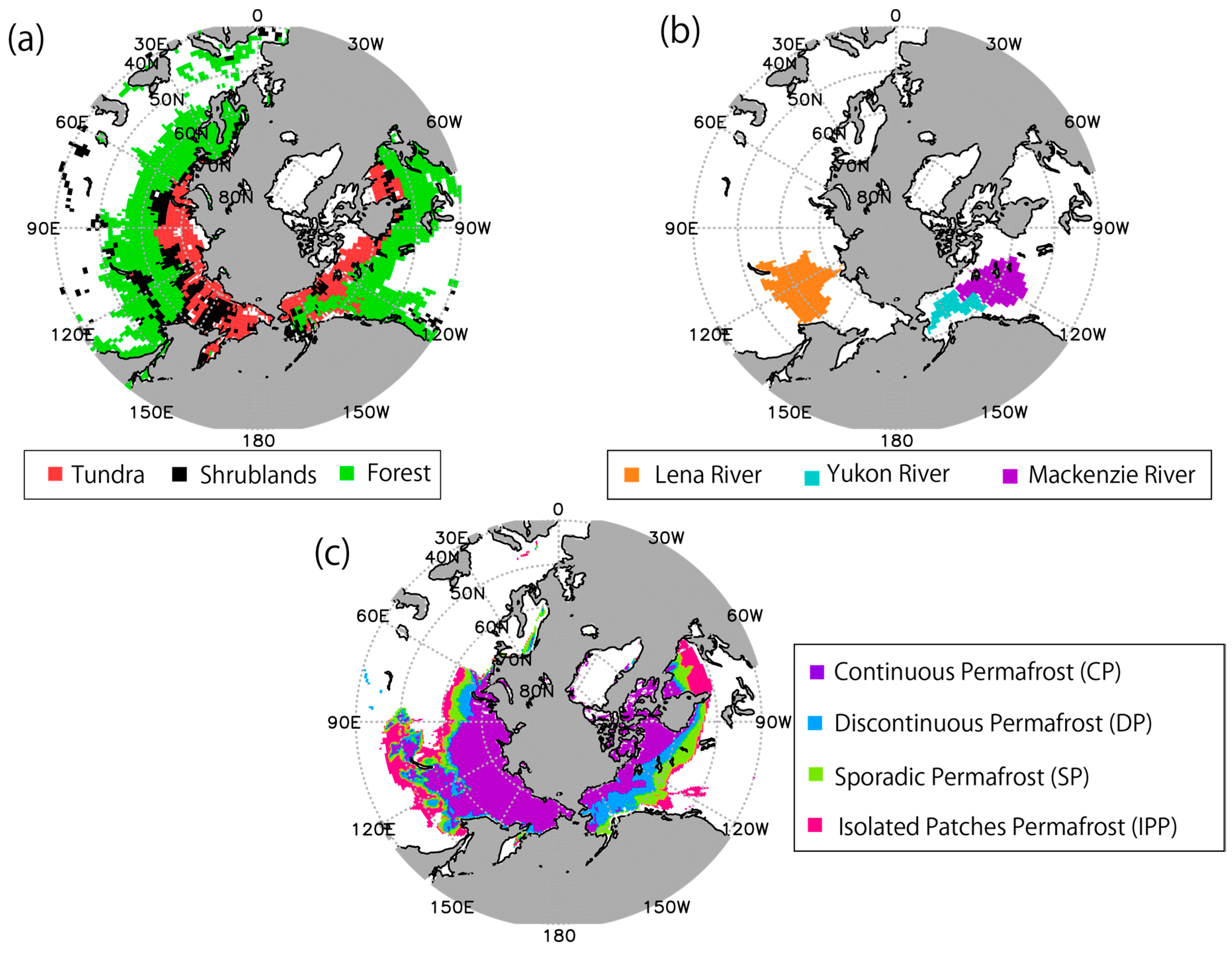
2.1. Study Area

Figure 1a shows a vegetation map. The red-colored area denotes the Arctic circumpolar tundra region (ACTR), which we defined using GLDAS and vegetation data obtained from the 1° GLDAS2/Noah Dominant Vegetation Type datasets (https://ldas.gsfc.nasa.gov/gldas/GLDASvegetation.php) using the NOAHv3.3 vegetation dataset from GLDAS2. In GLDAS, tundra regions are divided into three distinct types: bare ground tundra, mixed tundra and wooded tundra. However, bare ground tundra did not exist in the datasets. In this study, we only present data for wooded tundra to avoid the uncertainties associated with identifying mixed tundra along the narrow coastal areas of the Arctic Ocean, where it is difficult to distinguish between the ocean and land due to the coarse spatial resolution of GRACE data. In addition, we exclude from our analysis the areas in the ACTR that are within 300 km of glaciers and ice sheets (the masked-out areas in Figure 1a) to remove the effects of glacial and ice sheet melt on TWS anomalies. Therefore, in our analysis, the ACTR is delineated by the regions represented in red in Figure 1a. We, therefore, obtained a land area of approximately 5,527,630 km2 for the ACTR.
We calculated the distribution of permafrost throughout the ACTR based on the data obtained from the National Snow and Ice Data Center (NSIDC) website [16]. Approximately 83% of the ACTR is covered by continuous permafrost, while the rest is covered by discontinuous or sporadic permafrost (Figure 1c).
To understand the effects of river runoff on TWS anomalies on a basin-wide scale, we conducted an analysis of large pan-Arctic rivers at the basin scale. Long-term river runoff data are limited for large pan-Arctic river basins; however, sufficient data exist for three large catchments (Figure 1b and Table 1) that are suitable for a basin-scale analysis of the long-term trends in river runoff and TWS between 2002 and 2016. In terms of the whole basin-scale analysis, although we also excluded mixed tundra regions from the analysis (such an area was less than 1% within each basin area, and was therefore, negligible). we included mixed tundra, forests, and shrublands in the basin-scale analysis. The first catchment is the Lena River basin in eastern Siberia in the Russian Federation, which has an approximate area of 2430 × 103 km2, comprised largely of continuous permafrost (71%). The second is the Yukon River basin in Alaska, which has an area of 850 × 103 km2; it is underlain by both continuous permafrost (23.2%) and discontinuous permafrost (74.7%). The third catchment is the Mackenzie River basin in northern Canada, which covers an area of 1790 × 103 km2, 20.0% of which is underlain by continuous permafrost and 39.2% is underlain by discontinuous permafrost. These three basins are primarily covered by forests. In the Lena River basin, shrublands cover nearly 30% of the basin.

2.2. Data

2.2.1. Satellite Data

To quantify the TWS in the study region, we obtained the GRACE data (Level-2, Release 5) from three analysis centers: The University of Texas—Center for Space Research (CSR) and the Jet Propulsion Laboratory (JPL) in the United States and the GeoForschungZentrum Potsdam (GFZ) in Germany. Each dataset consists of 158 months of data collected between April 2002 and December 2016 spanning 15 northern hemisphere winters. Gaps in the dataset exist for 20 months during this time period: June 2002, July 2002, June 2003, January 2011, June 2011, May 2012, March 2013, August 2013, September 2013, February 2014, July 2014, December 2014, June 2015, October 2015, November 2015, April 2016, September 2016, and October 2016. These gaps were caused by instrumental problems and battery management issues (see the GRACE Science Data System Monthly Report, June 2017). Here, we did not apply any interpolation to cover the periods with no data. In our analysis, we used the ensemble mean of the three GRACE datasets (i.e., a simple arithmetic mean of the CSR, JPL, and GFZ datasets) as recommended by Sakumura et al. [17] and the official GRACE Science Data System. In doing so, we were able to reduce random errors and enhance common signatures included within each GRACE dataset.
The GRACE data used in this study express the Earth’s gravity field in the form of spherical harmonic coefficients (Stokes coefficients). These Stokes coefficients are estimated up to a degree and order of 60 or 96 depending on the analysis center and the observation period. Here, we truncated the Stokes coefficients at a degree and order of 60 (corresponding to a spatial resolution of ~300 km) because higher-frequency coefficients are especially contaminated by short wavelength noise from temporal aliasing errors [18]. In addition, we used filtering techniques to further reduce the sources of short wavelength noise. We applied a Gaussian filter with a radius of 240 km.
Since GRACE measurements are less sensitive to the global-scale components of the Earth’s gravity field, in particular, the degree-1 and zonal degree-2 components, which represent the geocentric motion and the Earth’s dynamic oblateness, respectively, it is common practice to complement these components with other space geodetic techniques or model estimates. Here, we used the degree-1 coefficients estimated by combining GRACE data with an ocean model [19] and the zonal degree-2 coefficients measured via satellite laser ranging (SLR) [20]. Subsequently, we converted the GRACE data into surface mass variations using the methods presented in [18]. A degree-1 load Love number (k1) of 0.021 was then used to convert the GRACE reference frame (the center of mass) into the center of the figure frame to make the data consistent with the GLDAS data [19]. Atmospheric and oceanic mass variations were removed during the processing of the original GRACE data. We also corrected the data for the effects of glacial isostatic adjustments, which contribute less than 2% to the GRACE signal within the region of interest [21], using the model proposed by Geruo et al. [22]. The long-term averages of the Stokes coefficients were removed from the monthly solutions to provide the surface mass variations, which represent the TWS anomalies relative to the static field. Hereafter, we refer to these TWS anomalies as TWS, which includes surface and subsurface water masses.
Here, we obtained the estimation errors of the GRACE linear EWT (Equivalent Water Thickness) trend by computing the room-sum-square value of the ordinary least squares (OLS) standard errors and the GRACE standard errors. The OLS standard errors were computed by assuming a regression model with linear and seasonal components. The GRACE standard errors were obtained by propagating the GRACE ETW errors [23] with the OLS estimator of a linear component [24]. According to our error analysis, the data are accurate within +/− 0.9 mm y−1.

2.2.2. Reanalysis Data

Global Land Data Assimilation System v1 (GLDAS1) products and newly produced reanalysis data from GLDAS v2 (GLDAS2) have been widely and effectively used to understand the temporal and spatial variabilities of TWS anomalies. Recently, Wang et al. [25] studied three Chinese river basins using estimates based on TWS data from the Gravity Recovery and Climate Experiment (GRACE) and GLDAS to compare products based on GLDAS1 and GLDAS2. They showed that bias corrections in the precipitation data based on the latter greatly reduced the biases relative to that based on the former. However, they also noted that the latter had larger mean absolute errors. Thus, it is important to assess the availabilities of products based on GLDAS1 and GLDAS2 for the Arctic tundra and pan-Arctic river basins in order to investigate better products with which to analyze TWS anomalies in the regions.
The GLDAS1 and GLDAS2 products [26] are used to calculate TWS anomalies and assess TWS estimates from GRACE data. In this study, to examine the uncertainty in the GLDAS1 products, we use a multi-model ensemble of GLDAS1 data consisting of four different land surface models: (1) the Noah land surface model (Noah) [27], (2) the Community Land Model (CLM) [28], (3) the variable infiltration capacity (VIC) model [29], and (4) the MOSAIC LSM (MOS) [30]. Each product has a monthly time step and a spatial resolution of 1.0° × 1.0°. Firstly, we calculated the TWS from each model product of GLDAS1 to avoid the complex treatment of different soil depth in each model. Soil depth (the number of soil layers) for Noah, CLM, VIC and MOS was 2.0 m (4 layers), 3.433 m (10 layers), 1.9 m (3 layers), and 3.50 m (3 layers), respectively. Thus, CLM had the most sophisticated soil layer model compared with the others. The TWS derived from the multi-model GLDAS1 ensemble was calculated from each model-based TWS. Its ensemble spread (the maximum and minimum range) provides a measure of the uncertainty in the land surface models of the GLDAS1 products. GLDAS2, which currently uses only the Noah LSM and employs the Princeton meteorological forcing dataset [31] as the only source of forcing data, was corrected using the observation-based datasets of precipitation, air temperature, and radiation. Here, we applied a low-pass filter to the GLDAS1 and GLDAS2 data to truncate the spherical harmonic components at a degree and order of 60. Additionally, a Gaussian filter with a radius of 240 km was applied to the GLDAS1 and GLDAS2 data to adjust them to the same spatial resolution as the GRACE data.
In this study, we use evapotranspiration and precipitation data from GLDAS1 and GLDAS2 datasets.

2.2.3. River Flow Rate Data (R)

The flow rate data for the estuaries of three major pan-Arctic rivers (the Lena, Mackenzie, and Yukon Rivers) were used to analyze the basin-scale variations in TWS. For the Lena River, we used the observations provided by R-ArcticNet (developed and maintained by the University of New Hampshire) for 2002–2009 and by the AHYST.Lena dataset [32,33] for 2010–2011, while data obtained from the Canadian hydrometric database (HYDAT) and the United States Geological Survey (USGS) website were used for the Mackenzie River from 2002 to 2015, and the Yukon River from 2002 to 2016, respectively.
For the Lena River, the runoff data were obtained from the Kusur hydrological station, located near the mouth of the river at 70.70°N, 127.65°E. The runoff data for the Yukon and Mackenzie rivers were obtained from the gauge stations at the river mouths, namely, from the Pilot station (61.93°N, 162.88°W) on the Yukon River and the Arctic Red River station (67.46°N, 133.75°W) on the Mackenzie River.

2.3. Theory

In this section, we outline the theoretical basis of our analysis. To evaluate the monthly TWS from the GRACE data, we use the water balance equation expressed by Suzuki et al. [12]:
Δ T W S = P d t E d t R d t = Δ SWE + Δ CS + Δ SM + Δ GW + Δ SW
where P is the monthly precipitation (mm month−1), E is the monthly evapotranspiration (mm month−1), R is the monthly river runoff from the basin (mm month−1), Δ SWE is the change in the snow water equivalent (mm month−1), Δ CS is the change in the total amount of water within the canopy (mm month−1), Δ SM is the change in the vertical accumulated soil moisture within the total soil layer (mm month−1), Δ GW is the change in the groundwater or ice within the permafrost (mm month−1), and Δ SW is the change in different surface water bodies (e.g., lakes, rivers, and wetlands; mm month−1). Hereafter, we refer to the TWS values determined using GRACE data as TWSGRACE.
The GLDAS-based TWS determination includes only Δ SWE, Δ CW, and Δ SM from Equation (1). Because Δ CW is a minor factor, the TWS determined from the GLDAS data depends primarily on Δ SWE and Δ SM. Hereafter, we refer to the TWS values determined from the GLDAS1 and GLDAS2 products as TWSGLDAS1 and TWSGLDAS2, respectively, and the P and E values determined from GLDAS1 and GLDAS2 are accordingly referred to as PGLDAS1, PGLDAS2, EGLDAS1, and EGLDAS2.

2.4. Analysis

2.4.1. TWS Changes Across the Arctic Circumpolar Tundra Region

We analyzed the temporal variations of TWS (i.e., from GRACE, GLDAS1, and GLDAS2) from 2002 to 2016 along with other variables (i.e., the temperature, precipitation, and evapotranspiration) for the entire ACTR. First, we examined the consistency among the TWS estimates from the GRACE, GLDAS1, and GLDAS2 datasets based on the coefficients of determination (R2) and differences in linear trends. Second, we analyzed the possible mechanisms for the changes in the mean annual TWS of the ACTR by comparing the TWS estimates against other hydrological and climate components. Note that the mean annual TWS is simply the average of available monthly TWS data over all possible years because some monthly TWS data were missing from the overall dataset as shown in Section 2.2.1. However, the mean annual TWS could not be calculated for 2002 because of insufficient data (less than nine months). We also analyzed the spatial variations in the linear TWS trends to identify the consistencies among the linear trends of TWSGRACE and various hydro-meteorological factors (precipitation and evapotranspiration) from the GLDAS1- and GLDAS2-based products.
Statistical analyses were conducted using nonparametric methods based on the approach by Ichii et al. [34] because these technique do not require an assumption of normality in variance, and are more robust against anomalous outliers. The slopes of the trends were calculated based on the Theil-Sen slope [35]. To test the significance of the trend, we used the Mann-Kendall trend test [36]. In addition, all correlation analyses were based on Kendall’s rank-correlation coefficients (Kendall’s τ) [36]. All statistical tests that were conducted had a significance level of p < 0.05.

2.4.2. TWS Changes Among the Three River Basins

Similar to the analysis performed for the ACTR in Section 2.4.1, we analyzed the temporal variations of all variables from 2002 to 2016 among the three river basins. We also used the river runoff data to explore the relationship between TWS and river runoff. Based on previous work [12,37,38], we hypothesize that the conditions during autumn and winter will affect river runoff in the subsequent year. To test this hypothesis, we calculated the correlations between the TWS values from July of one year and those from June of the following year along with those for the annual river runoff using available data. We calculated the monthly lag correlation coefficient (rLAG) for the annual river runoff data between 2002 and 2011 for the Lena River. We also calculated rLAG between 2002 and 2015 for the Mackenzie River using monthly TWS averages from September to December and annual river runoff estimates from the subsequent year as well as monthly TWS estimates from January to May and annual river runoff values for the same year.
All statistical analyses were based on the same approach described in Section 2.4.1.

3. Results

3.1. TWS in the Arctic Circumpolar Tundra

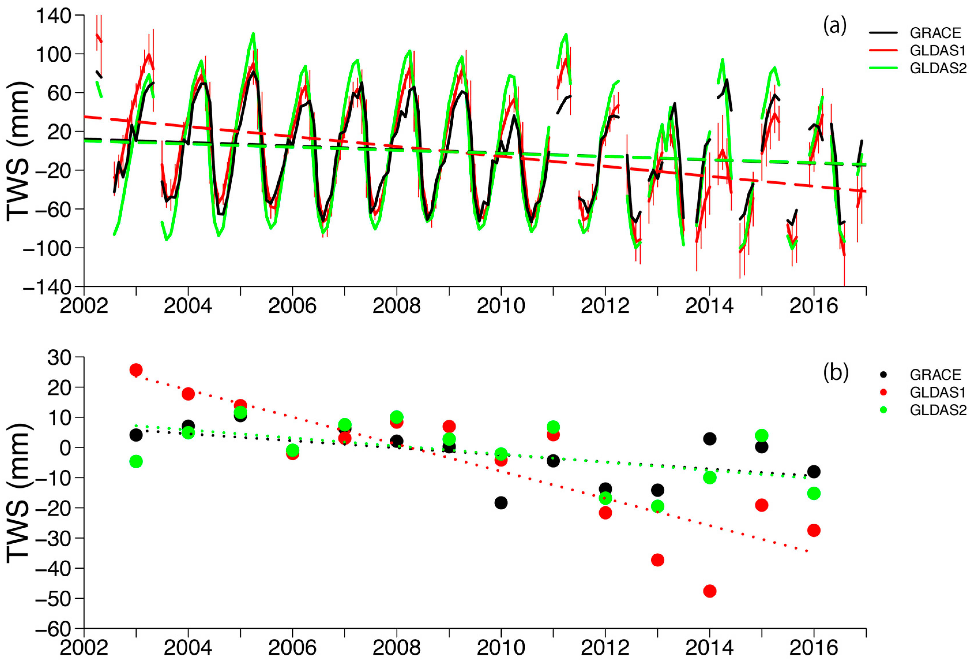
3.1.1. Temporal Variations in the TWS in the ACTR

Figure 2a illustrates the temporal variations in monthly TWS estimates averaged across the ACTR from GRACE, GLDAS1, and GLDAS2 datasets. From 2002 to 2016, the GRACE, GLDAS1, and GLDAS2 TWS datasets exhibited negative trends of −1.8 mm y−1 (τ = −0.11, p = 0.0340), −5.1 mm y−1 (τ = −0.25, p < 0.0001), and −1.6 mm y−1 (τ = −0.06, p = 0.2382), respectively. TWSGRACE and TWSGLDAS2 show the best agreement in linear trends (τ = 073, p < 0.0001), despite the larger seasonal amplitude in TWSGLDAS2 due to a larger winter TWS. These rates of decline exceed the uncertainty of −0.9 mm y−1 associated with TWSGRACE; thus, confirm the ability of the GRACE-based TWS data to reflect temporal trends in the ACTR.
The TWSGRACE data are also highly correlated with TWSGLDAS1 (τ = 073, p < 0.0001) despite the substantially larger rate of decline associated with GLDAS1 (−5.1 mm y−1). The values of R2 between TWSGRACE and TWSGLDAS1 (R2 = 0.81, p < 0.0001) and between TWSGRACE and TWSGLDAS2 (R2 = 0.85, p < 0.0001) indicate the degree to which the variations can be explained with a linear model. Based on these strong correlations among the three TWS datasets, we calculated a TWS change of more than 80% at the ACTR-scale using the GLDAS products, allowing us to determine the primary factor controlling the changes in TWSGRACE. The similarities among the three datasets imply that, similar to TWSGLDAS1 and TWSGLDAS2, TWSGRACE also largely depends on SWE and SM parameters. Even so, the negative trend in TWSGLDAS1 is nearly three times larger than the trends in TWSGRACE and TWSGLDAS2, which are very similar to each other. Overall, the inter-annual variations in TWSGRACE can be best explained by the GLDAS2 dataset.
The mean annual TWS is plotted in Figure 2b for all years except 2002 when insufficient data were available (less than nine months). In these smoothed datasets, TWSGRACE was more strongly correlated with TWSGLDAS2 (τ = 0.52, p = 0.0098) than with TWSGLDAS1 (τ = 0.45, p = 0.0264). TWSGRACE, TWSGLDAS1, and TWSGLDAS2 decreased by −1.2 mm y−1 (τ = −0.45, p = 0.0375), −4.5 mm y−1 (τ = −0.71, p = 0.0005), and −1.3 mm y−1 (τ = −0.34, p = 0.1005), respectively. Thus, the long-term trends observed in the mean annual TWSGRACE were consistent with those observed in TWSGLDAS2. Overall, these TSW data showed a decrease throughout the ACTR between 2002 and 2016, thereby providing evidence that hydrological changes are not only limited in the downstream of the Lena River basin, as reported in [12] but also are expanding throughout the whole ACTR.

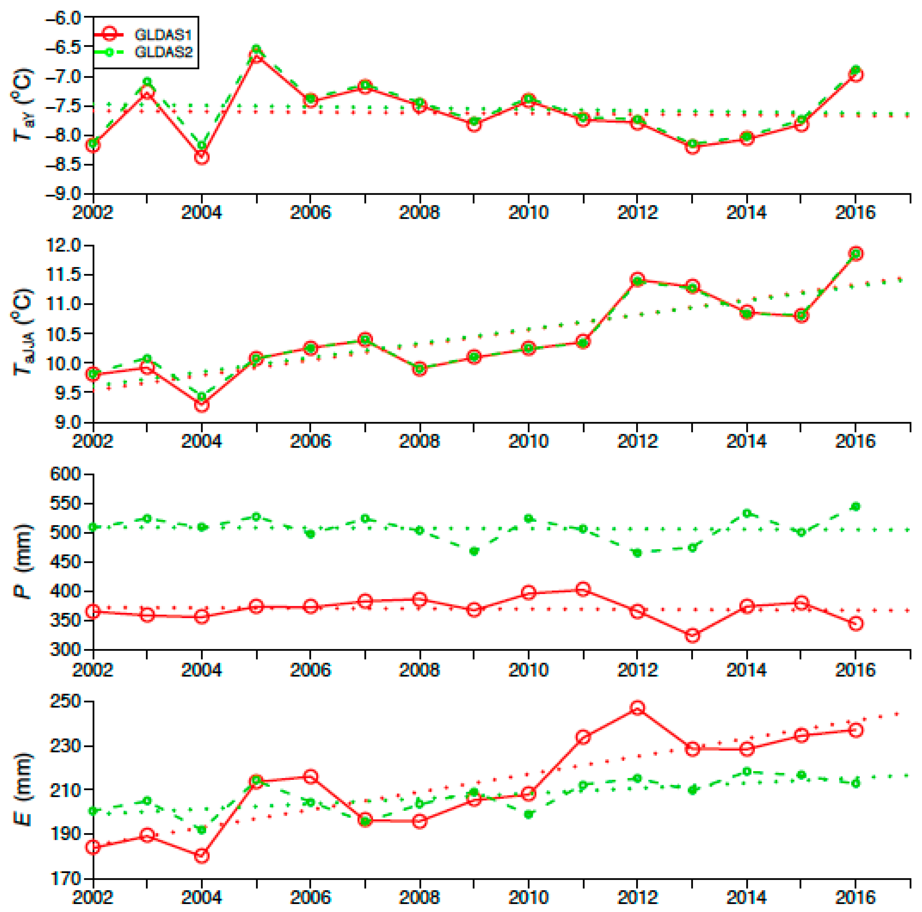
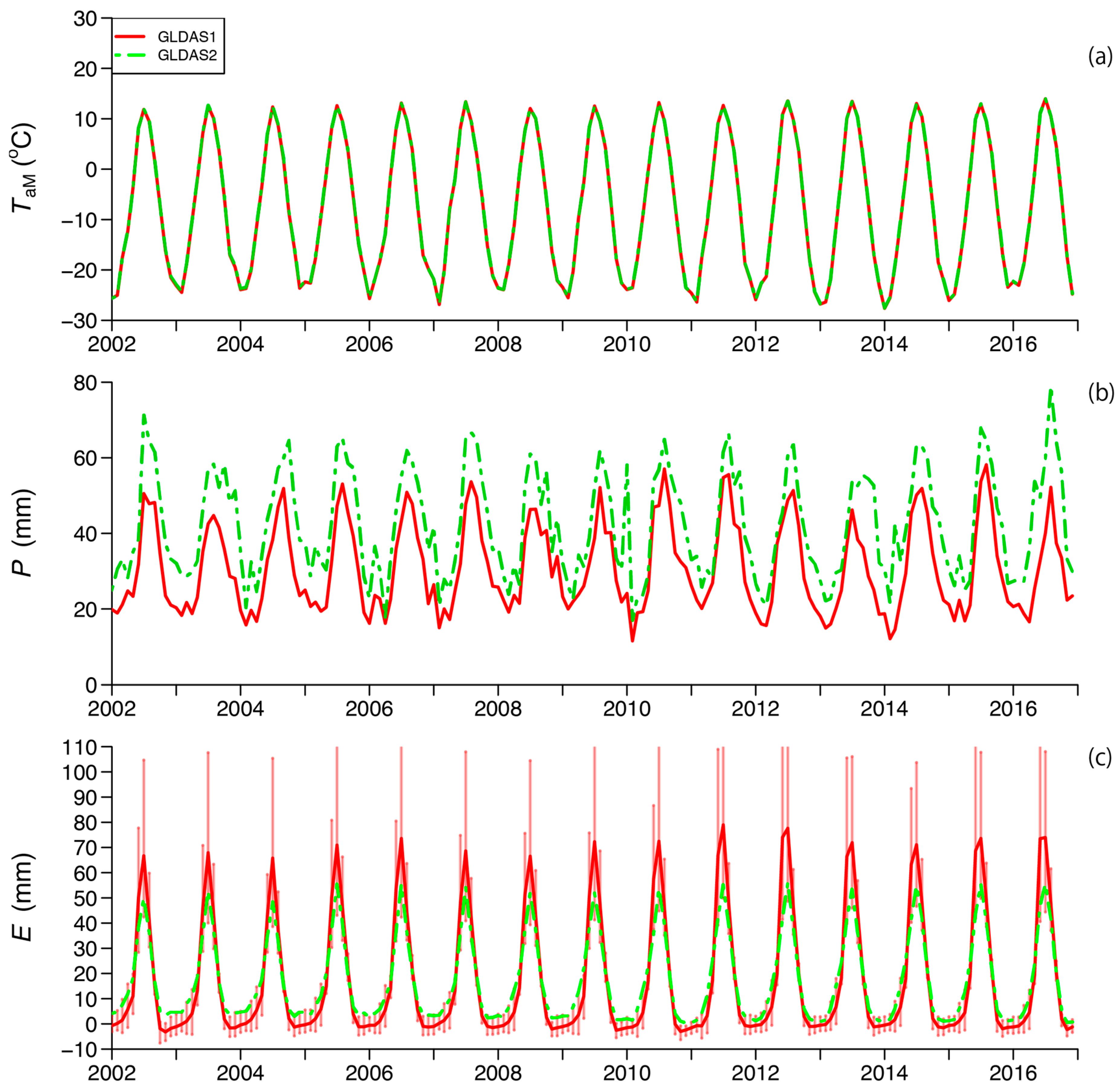
3.1.2. Precipitation, Evapotranspiration, and Air Temperature from GLDAS

We present the monthly air temperature (Ta), precipitation (P), and evapotranspiration (E) derived from the GLDAS1 and GLDAS2 datasets and assess their effects on the mean annual TWSGRACE (Figure 3). The 2-m air temperatures in the ACTR from the GLDAS1 data were very close to those calculated from the GLDAS2 data (Figure 3a, τ = 0.96, p < 0.0001). However, GLDAS2 produced p-values that are consistently higher than GLDAS1 (the bias (GLDAS1 − GLDAS2) = −11.4 mm month−1, τ = 0.77, p < 0.0001), while the inter-annual variability in E produced from GLDAS1 was larger than that observed from GLDAS2 (Figure 3c, τ = 0.95, p < 0.0001) owing to the higher (lower) E values in summer (winter). However, these differences cancel out when we calculate the all-term-averaged bias and are within the range of uncertainty associated with the various LSMs, as indicated by vertical red bars in Figure 3c.

3.1.3. TWSGRACE versus Ta, P, and E

To identify the possible forcing mechanisms of the mean annual TWS in the ACTR, we compared the mean annual TWSGRACE (Figure 2b) with the mean annual and summer (JJA) 2-m air temperature (Figure 4a and Figure 4b, respectively), the mean annual P (Figure 4c), and the values of E (Figure 4d). While there was no discernible trend in the mean annual temperature throughout the ACTR during this period, the JJA mean air temperature increased by approximately 0.13 °C y−1 (τ = 0.68, p = 0.0005) for GLDAS1 and 0.12 °C y−1 (τ = 0.66, p = 0.0008) for GLDAS2. However, no discernible trends were observed in P despite a slight decrease between 2005 and 2013.
The GLDAS1- and GLDAS2-based E increased steadily from 2002 to 2016 with slopes of approximately 4.1 mm y−1 for EGLDAS1 (τ = 0.66, p = 0.0008) and 1.2 mm y−1 for EGLDAS2 (τ = 0.49, p = 0.0133). The increase in E from either GLDAS dataset can explain most of the decrease in TWSGRACE shown in Figure 2b.
Thus, evapotranspiration driven by increasing summer temperatures may be the primary factor controlling TWSGRACE. This suggests that future warming might further decrease the TWS at high latitudes in the Arctic circumpolar region.

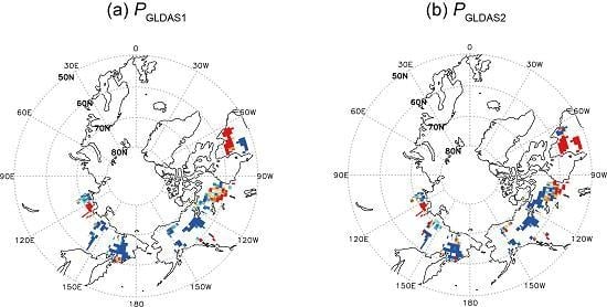
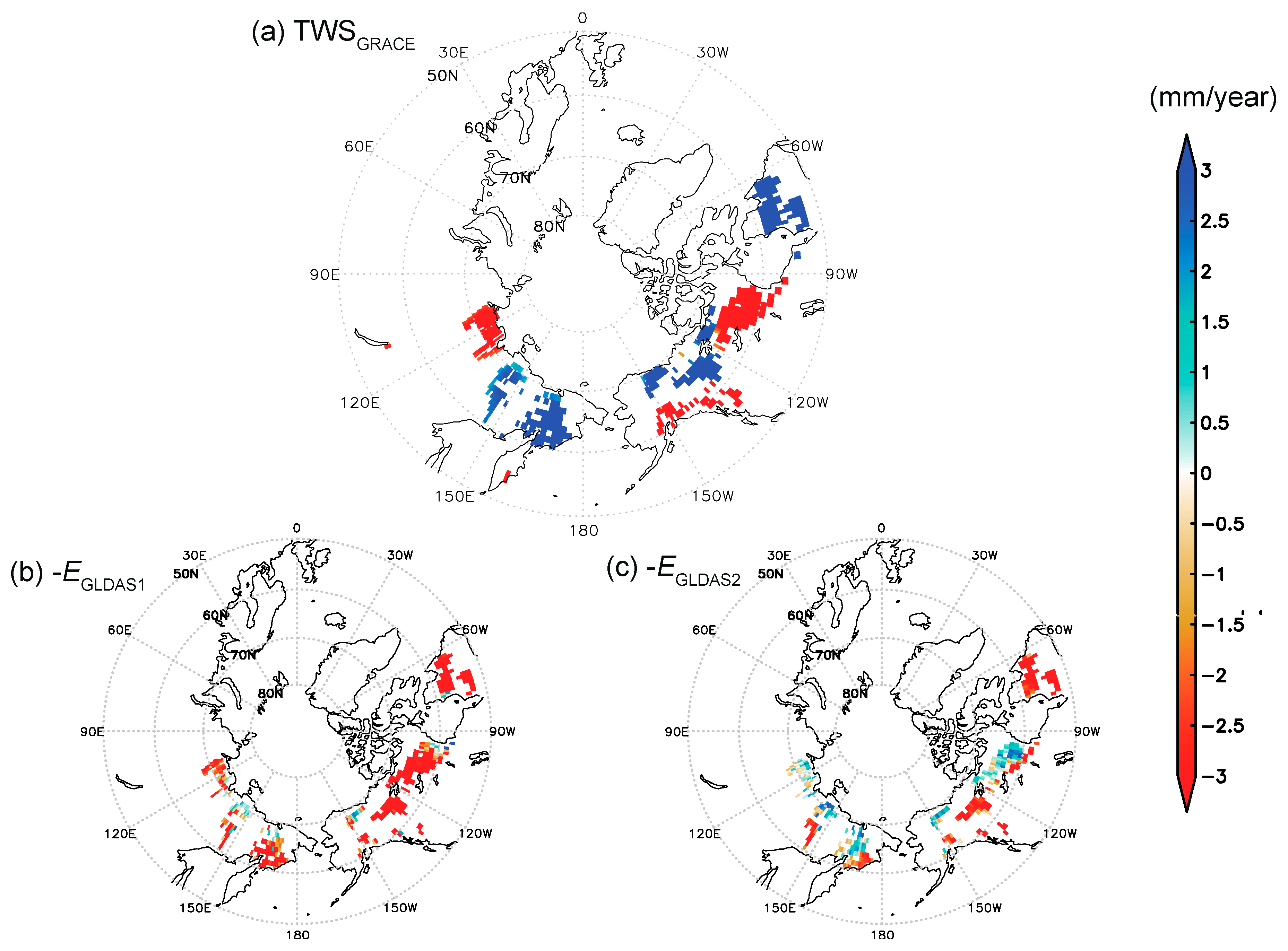
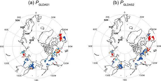
3.1.4. Regional Trends in TWS, P, and E

Here, we consider the regional trends in the mean annual TWS, P, and E from both GLDAS1 and GLDAS2. Figure 5a shows the spatial distribution of the trends in the annual TWS from 2002 to 2016 across the ACTR. There is an evident regional variation throughout the ACTR and a declining TWS in the high Arctic near the Lena River basin. The trends shown in Figure 5a are statistically significant (p < 0.05). Higher correlation coefficients are observed in North American Continent. A significant negative trend in TWS is mainly observed along the Gulf of Alaska and the Northwestern Territory in Canada. Meanwhile, the negative trends in TWS in the Eurasian Continent were weaker than those in the North American Continent.
To further understand these regional trends across the ACTR, we examined the distributions of E and P using the mean annual datasets from GLDAS1 and GLDAS2 (Figure 5b,c and Supplementary Figure S1a,b). The spatial variations in PGLDAS1 and PGLDAS2 and in EGLDAS1 and EGLDAS2 can be explained by the differences in the forcing data and in land surface models in GLDAS1 and GLDAS2. The all trends shown in colored area (Figure 5a–c and Supplementary Figure S1a,b) are statistically significant (p < 0.05).
Table 2 lists the correlation coefficients between the linear trends of TWSGRACE with the P and E estimates from both GLDAS1 and GLDAS2 in regions where TWSGRACE either increased or decreased (Figure 5a). The results are further differentiated according to the magnitude of the increase or decrease in TWSGRACE, namely, values from 0 mm y−1 and values of greater than or equal to 0 mm y−1. The reasonable correlation coefficients are observed between TWSGRACE and E for both GLDAS1 and GLDAS2. This confirms that E dominates the spatial distribution of TWSGRACE.
Negative correlations are observed between TWSGRACE and P. Thus, P does not explain TWS variations. This relationship is similar to the ACTR-averaged results in Figure 4. Similarly, PGLDAS2 and EGLDAS2 are more strongly correlated with TWSGRACE than PGLDAS1 and EGLDAS1.
Overall, these results suggest that changes in E throughout the ACTR are the primary driver of TWSGRACE variations from 2002 to 2016. In addition, the GLDAS1-based TWS, P, and E products exhibit poor correlations with the GRACE-based TWS. Thus, in the following sections, we use GLDAS2-based products only.

3.2. Whole Basin-Scale Variabilities in the TWS for Three Arctic Rivers

Here, we present the TWS dataset for the Lena, Yukon, and Mackenzie rivers and assess the variability in TWS in relation to river runoff rates and other parameters.

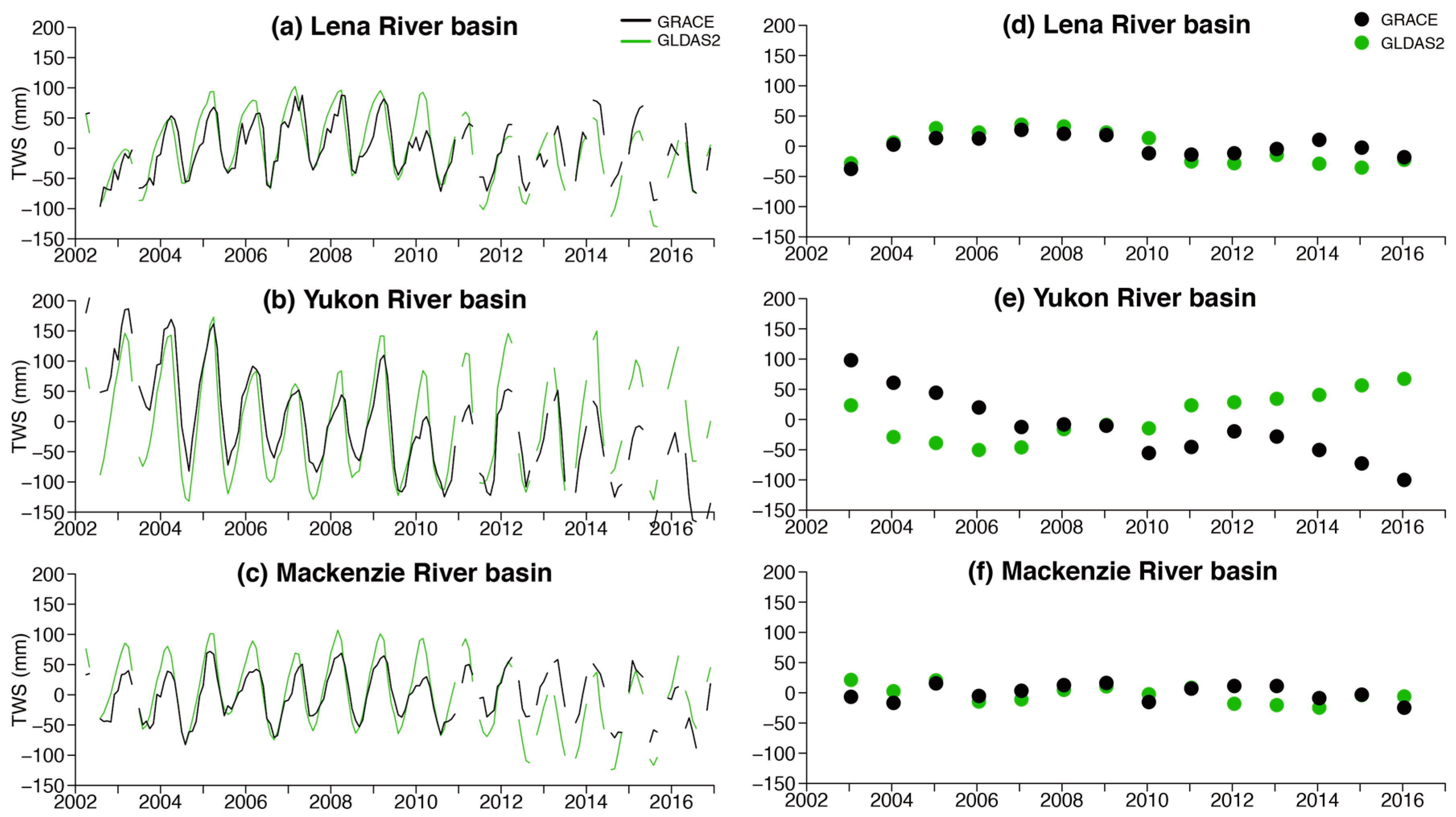
3.2.1. Temporal Variations

To evaluate the impacts of river runoff on three of the largest Arctic catchments, we analyzed the entire basin-scale changes in monthly TWS from 2002 to 2016 for the Lena, Yukon, and Mackenzie River Basins (Figure 6a–c). No significant trend is evident in either the Lena or Mackenzie rivers, while a negative trend in the TWSGRACE is observed in the Yukon River basin.
To understand the temporal variations in TWSGRACE using GLDAS2-based products, we compared TWSGRACE to TWSGLDAS2. The τ and p-values between TWSGRACE and TWSGLDAS2 were for the Lena River (τ = 0.65, p < 0.0001), Yukon River (τ = 0.52, p < 0.0001), and Mackenzie River (τ = 0.60, p < 0.0001) basins. We found statically significant correlation between TWSGRACE to TWSGLDAS2. Therefore, in order to understand TWS variations in each basin, we can use each hydrological component from GLDAS2 for the following analysis.
The mean annual TWS is plotted in Figure 6d–e for all years except 2002 when insufficient data were available (less than nine months). Although annual mean values of TWSGRACE and TWSGLDAS2 in the Lena and Mackenzie River basins did not show any trends as well as monthly datasets, annual mean TWSGRACE in the Yukon River basin decreased by about −13 mm y−1 (τ = −0.45, p < 0.0001), while the annual mean TWSGLDAS2 had no decreasing trend. Thus, the long-term trends observed in the mean annual TWSGRACE in the Yukon were not consistent with those observed in TWSGLDAS2. However, the p-value between TWSGRACE and TWSGLDAS2 for the Yukon was 0.039, and indicated a statistically significant correlation.

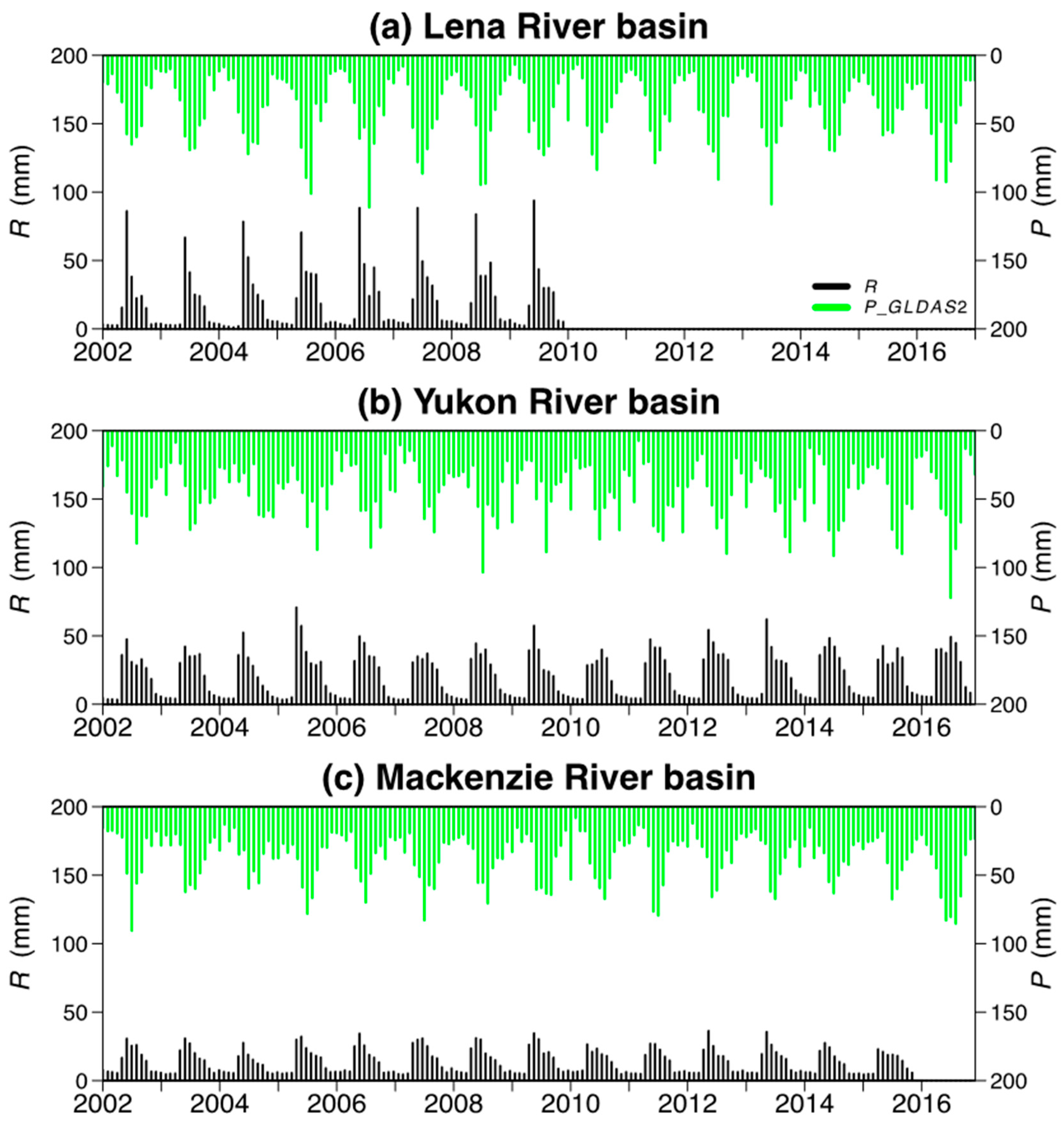
3.2.2. Monthly Mean P and R

Figure 7 shows the temporal variations in the monthly basin-averaged precipitation (PGLDAS2) and river runoff rates of each river basin. The maximum monthly P occurred in July for the Lena and Mackenzie River basins (Figure 7a,c) and in June or July for the Yukon River basin (Figure 7b). The Lena River exhibits the largest amount of river runoff (R), followed by the Yukon River and the Mackenzie River. The peak value of R occurred in June for all three rivers. Using monthly climatology of river runoff data, the peak snowmelt occurs between April and June, accounting for approximately 40%, 36%, and 28% of the annual R in the Lena River, Yukon River, and Mackenzie River basins, respectively.
In terms of the whole basin-scale analysis, we used the same units for the TWS, R, and E. The TWS is the annual mean, and P and E are the annual integration. Thus, these variations have the same order of magnitude. The comparison of R with TWS among the three river basins reveals strong positive correlations for the Lena River and Mackenzie River basins but no significant correlation for the Yukon River basin, where TWS was sensitive to the changes in EGLDAS2 (Figure 8). This confirms E as a driving factor in the decline in TWS in the Yukon River catchment. Here, we consider only the GLDAS2-based E data because of the greater consistency between the GLDAS2 and GRACE products.

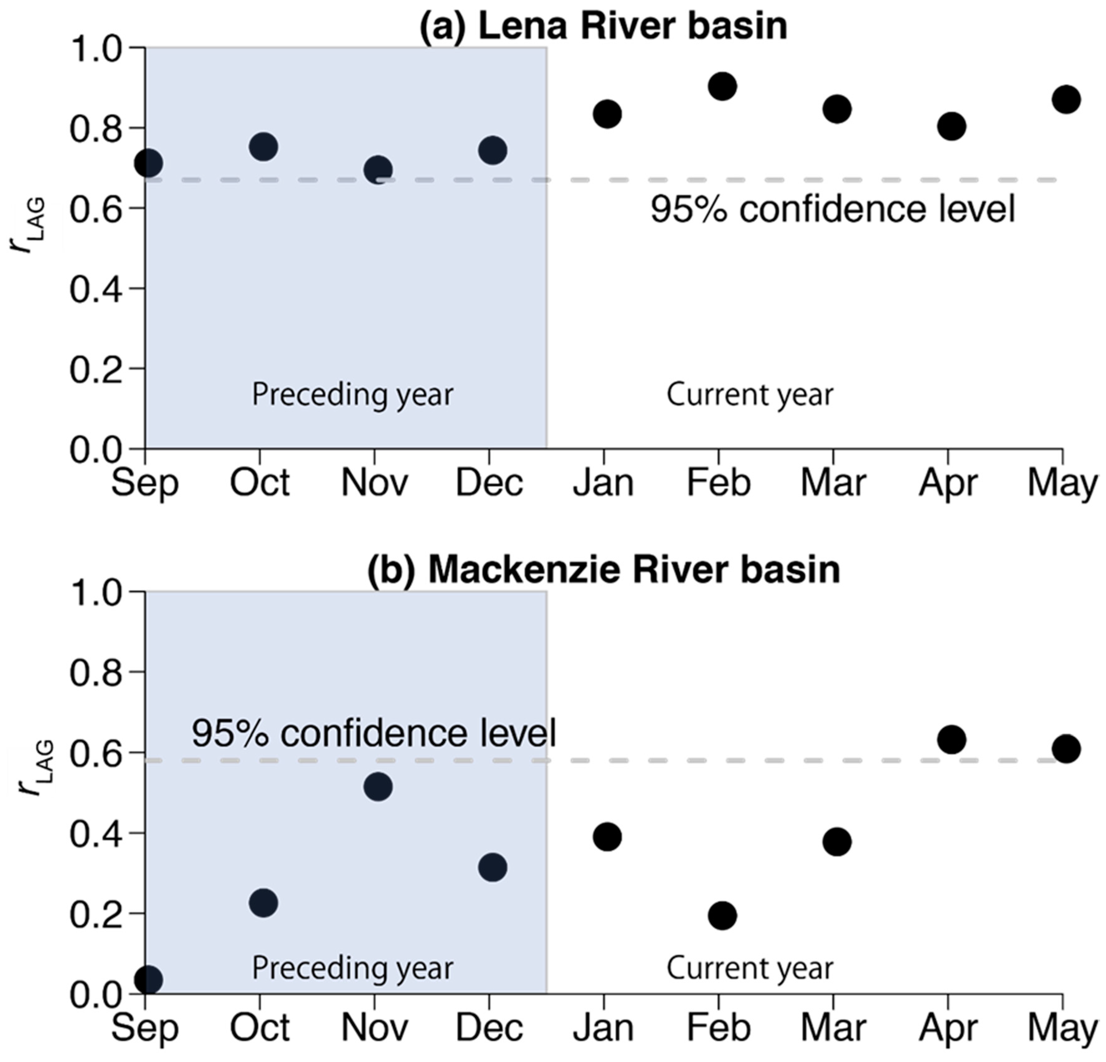
3.2.3. Relationship between the TWS and Runoff in the Lena and Mackenzie River Basins

We examine rLAG as defined in Section 2.4 to further investigate the correlation between TWS and runoff in the Lena and Mackenzie River basins. We do not consider the TWS of the Yukon River basin because it did not correlate with river runoff.
Statistically significant increases in rLAG are observed in September in the Lena River basin and in April in the Mackenzie River Basin (Figure 9). The maximum rLAG corresponds to TWS in February for the Lena River Basin and in April for the Mackenzie River, suggesting that the conditions in previous autumn and winter affected only the river runoff in continuous permafrost basins, such as those in the Lena River. Only a small portion of the Mackenzie River basin is covered by continuous permafrost; nearly half of the basin is free of permafrost. Therefore, the high rLAG value in autumn within the Lena River basin indicates that the autumn TWS can serve as a climatic signature for permafrost-dominated river runoff in any given year, as was noted by Suzuki et al. [12]. The influence on the autumn TWS from the preceding year is evident, despite the inclusion of the snow water equivalent over the land. However, in basins such as the Mackenzie River, which are not dominated by permafrost, the TWS from the preceding year had no effect on the river runoff of the following year.

4. Discussion

4.1. Hydrological Changes in the Tundra Throughout the ACTR

Through our results, the GRACE-based TWS record shows a clear decrease in the TWS throughout the ACTR and that the JJA air temperature increased. The previous GRACE-based TWS trends in eastern Siberia [21] and in the three largest Siberian river basins (i.e., the Lena, Yenisey, and Ob River basins) [39] all showed positive trends using shorter data periods (e.g., 5 or 8 years) than the present study. In addition, Huang et al. [11] showed that the aridity of most of the Artic region, including eastern Siberia and the North American continent, will increase in this century using data from the CMIP5. Our results, which indicated decreasing trends of the TWS in eastern Siberia and the North American continent, correspond to those of Huang et al. [11]. Furthermore, using the CMIP5 dataset, Cook et al. [40] demonstrated that the expansion of dry areas can be attributed to globally widespread increases in the potential evapotranspiration while the spatial heterogeneous response of the precipitation can be used to define the drying and wetting patterns over the global land surface. Their conclusions confirm our results, i.e., that the TWS in the ACTR is driven by increasing evapotranspiration. Although Boike et al. [41] reported no warming trends over an island in the Lena Delta from the summer of 1998 to the summer of 2011, they showed that the warmest summer occurred in 2010 Thus, we propose that the TWS in the ACTR is driven by increasing summer air temperatures and evapotranspiration. Some previous studies [42,43] showed that aridity of the land could be related to atmospheric warming. An increase in the aridity throughout the ACTR might accelerate the warming air temperature trend in the Arctic. Overall, our results have implications for understanding future trends in the TWS, which could be expected to continue to decline as the Arctic continues to warm due to climate change.

4.2. Whole Basin-Scale Hydrological Changes

Except for the Yukon River, we found a clear relationship between the TWS anomalies and river runoff. Walvoord and Kurylyk [15] showed that continuous permafrost prevents infiltration into the deeper soil layer while some of the subsurface water in discontinuous permafrost regions is connected to the groundwater and will thus increase the subsurface flow. Thus, all of the TWS accumulated during autumn and winter increases the amount of R in the Lena River Basin; however, continuous permafrost is scarce in the Mackenzie River basin, and most of the TWS can cause subsurface flow and change the TWS during a winter. Overall, as the continuous permafrost distribution decreases, the response of river runoff to precipitation will be accelerated and the role of the TWS as a climate record will be diminished.
Next, we discuss the possible causes for the GRACE-based TWS trend in the Yukon River basin. The Yukon River basin is located in a transition zone from continuous to discontinuous permafrost and is mostly underlain by an unstable discontinuous permafrost zone. Just as we found a strong negative trend in the GRACE-based TWS in the Yukon River basin, Nitze et al. [13] showed a net lake area loss of 2.8% in Alaska. The abundance of disappearing lakes in the discontinuous permafrost regions of Central Alaska [44] has been linked to an increased connectivity to the groundwater supply [45]. Permafrost degradation or disappearance along the continuous-discontinuous permafrost interface could represent a good explanation for the strong decreasing TWS trend in the Yukon River basin. The low correlation coefficient between TWSGRACE and TWSGLDAS2 can be explained by permafrost degradation. Several research investigations [44,46] showed that an increased evapotranspiration was responsible for observed lake area losses in central Alaska and the Yukon Flats. Those research results correspond well with our findings of a high correlation between the TWS and evapotranspiration and of no correlation between the TWS and river runoff in the Yukon River basin. Therefore, a negative trend in the GRACE-based TWS within the Yukon River basin and the low correlation coefficient between TWSGRACE and TWSGLDAS2 can be explained by permafrost degradation and evapotranspiration, although further research is needed to investigate the details of the TWS changes in the Yukon River basin. Overall, permafrost degradation and increased evapotranspiration in the Yukon River basin could have caused the decreasing GRACE-based TWS trend from 2002 to 2016 because of the unstable discontinuous permafrost distribution throughout most of the Yukon River basin.

4.3. Inconsistencies between GLDAS1 and GLDAS2

The main difference between GLDAS1 and GLDAS2 was due to the variation in forcing meteorological factors, as GLDAS2 employs the Princeton meteorological forcing dataset [29]. Our analyses demonstrated a greater consistency between TWSGRACE and the TWSGLDAS2 product than the TWSGLDAS1 data throughout the ACTR.
However, there are also significant differences between the GLDAS products. For example, the values of P in GLDAS2 exceed those in GLDAS1, although the air temperatures are consistent between the two products. Combined with the stronger spatial correlation coefficients between TWSGRACE and PGLDAS2 (Table 2), we suggest that the GLDAS2 products are more suited for pan-Arctic hydrological analyses than GLDAS1. In addition, EGLDAS2 demonstrated a higher correlation with the spatial trends in the GRACE-based TWS. However, the linear trend in EGLDAS1 was much larger than that in EGLDAS2 with nearly ubiquitous negative trends over the ACTR. These results correspond with the results of Wang et al. [25], who showed that EGLDAS1 overestimated the evapotranspiration relative to EGLDAS2.
However, one drawback with regard to the current GLDAS2 product is that it is based solely on the Noah LSM; meanwhile, GLDAS1 uses multiple land surface models. This allows GLDAS1 to provide greater evaluations of model uncertainties. For instance, EGLDAS2 falls within the ensemble spread of EGLDAS1 despite the different forcing data of GLDAS1 and GLDAS2. In addition, we found that the GLDAS1-based TWS using a sophisticated LSM (e.g., the CLM) had a much higher correlation with the GRACE-based TWS than that using a simple LSM utilizing a single-layer snow and vegetation model (e.g., the Noah LSM). Thus, the ensemble spread of the GLDAS1-based product reflects some parameter uncertainties in the LSMs. Moreover, the GLDAS1-based product using a sophisticated LSM could correspond more effectively to the GRACE-based TWS.

5. Conclusions

We present a record of the GRACE-derived TWS in the Arctic circumpolar tundra region (ACTR) and in the three largest pan-Arctic river basins from April 2002 to December 2016. Using the multi-model ensemble of reanalyzed data from GLDAS1 and the newly developed reanalyzed data from GLDAS2, including other key parameters such as Ta, P, and E, we find the following conclusions:
  • The negative trend in the TWS throughout the ACTR was primarily driven by evapotranspiration. Meanwhile, precipitation has a minor impact on the TWS.
  • In terms of regional changes in the TWS, a large and significant negative trend in the TWS can be observed mainly over the North American continent, including the region along the Gulf of Alaska and the Northwestern Territory of Canada. Meanwhile, the negative trends in the TWS over the Eurasian continent were weaker than those over the North American continent.
  • The comparison of R with TWS among the three river basins reveals strong positive correlations for the Lena River and Mackenzie River basins, but no significant correlation for the Yukon River basin, where TWS was sensitive to the changes in EGLDAS2. This confirms E as a driving factor in the decline in TWS, even on the scale of the whole basin.
  • The TWS among the three river basins was further controlled by the presence of continuous permafrost. For example, the autumnal TWS in the Lena River Basin (which exhibits continuous permafrost) persisted through the spring of the following year. However, no such effect was observed in the Mackenzie River catchment, which is partially covered in both continuous permafrost and discontinuous permafrost.
  • The GLDAS2-based products corresponded better with the spatiotemporal variability in TWSGRACE than the GLDAS1-based products. GLDAS2 is likely more suitable for analyzing hydrological changes in Arctic regions than GLDAS1.
To improve our understanding of the Arctic freshwater cycle, additional GRACE data regarding river runoff is required. In particular, the TWSGRACE data in the Yukon River clearly indicated a negative trend in our analysis, and the data were not affected by river runoff. Although this corroborates the negative TWS trends as strongly related to evapotranspiration throughout the ACTR and in the Yukon River Basin, the mechanism for this is still unknown and should represent the focus of future research. Overall, we assume that the negative trend of TWS could be expected to continue in the future due to further warming conditions during the summer season at high latitudes, leading to substantial reductions in the TWS throughout the Arctic.

Supplementary Materials

The following are available online at https://www.mdpi.com/2072-4292/10/3/402/s1, Figure S1: The spatial variations in PGLDAS1 (a) and PGLDAS2 (b).

Acknowledgments

Portions of this study were supported by a Grant-in-Aid for Scientific Research (C) (No. 16K00581) and a Grant-in-Aid for Challenging Exploratory Research (No. 25550022). In addition, this study was partly carried out by the Joint Research Program of the Institute for Space-Earth Environmental Research (ISEE), Nagoya University. We thank the four anonymous reviewers for their contributions to improving the first draft of this article.

Author Contributions

K.S., K.I., Y.I. and T.H. conceived and designed this study; K.S. and K.M. analyzed the data; K.M. and Y.Y. contributed materials and analysis tools; K.S., K.M., F.P., K.I., Y.I. and T.H. wrote the paper. All authors discussed and reviewed the manuscript.

Conflicts of Interest

The authors declare no conflict of interest. The founding sponsors had no role in the design of the study; in the collection, analyses, or interpretation of data; in the writing of the manuscript, and in the decision to publish the results.

References

  1. Serreze, M.C.; Barrett, A.P.; Slater, A.G.; Woodgate, R.A.; Aagaard, K.; Lammers, R.B.; Steele, M.; Moritz, R.; Meredith, M.; Lee, C.M. The large-scale freshwater cycle of the arctic. J. Geophys. Res. Oceans 2006, 111. [Google Scholar] [CrossRef]
  2. Chapin, F.S., III; Sturm, M.; Serreze, M.C.; McFadden, J.P.; Key, J.R.; Lloyd, A.H.; McGuire, A.D.; Rupp, T.S.; Lynch, A.H.; Schimel, J.P.; et al. Role of land-surface changes in Arctic summer warming. Science 2005, 310, 657–660. [Google Scholar] [CrossRef] [PubMed]
  3. Peterson, B.J.; Holmes, R.M.; McClelland, J.W.; Vörösmarty, C.J.; Lammers, R.B.; Shiklomanov, A.I.; Shiklomanov, I.A.; Rahmstorf, S. Increasing river discharge to the Arctic ocean. Science 2002, 298, 2171–2173. [Google Scholar] [CrossRef] [PubMed]
  4. Shiklomanov, A.I.; Lammers, R.B. Record Russian river discharge in 2007 and the limits of analysis. Environ. Res. Lett. 2009, 4, 045015. [Google Scholar] [CrossRef]
  5. Rawlins, M.A.; Ye, H.; Yang, D.; Shiklomanov, A.; McDonald, K.C. Divergence in seasonal hydrology across northern Eurasia: Emerging trends and water cycle linkages. J. Geophys. Res. Atmos. 2009, 114. [Google Scholar] [CrossRef]
  6. Willmott, C.J.; Matsuura, K. Terrestrial Air Temperature and Precipitation: Monthly and Annual Time Series. Available online: http://climate.geog.udel.edu/~climate/html_pages/README.ghcn_ts2.html (accessed on 17 November 2017).
  7. St Jacques, J.-M.; Sauchyn, D.J. Increasing winter baseflow and mean annual streamflow from possible permafrost thawing in the Northwest Territories, Canada. Geophys. Res. Lett. 2009, 36, 53–56. [Google Scholar] [CrossRef]
  8. Quinton, W.L.; Hayashi, M.; Pietroniro, A. Connectivity and storage functions of channel fens and flat bogs in northern basins. Hydrol. Process. 2003, 17, 3665–3684. [Google Scholar] [CrossRef]
  9. Papa, F.; Prigent, C.; Rossow, W.B. Monitoring flood and discharge variations in the large Siberian rivers from a multi-satellite technique. Surv. Geophys. 2008, 29, 297–317. [Google Scholar] [CrossRef]
  10. Hood, J.L.; Hayashi, M. Characterization of snowmelt flux and groundwater storage in an Alpine headwater basin. J. Hydrol. 2015, 521, 482–497. [Google Scholar] [CrossRef]
  11. Huang, J.; Yu, H.; Guan, X.; Wang, G.; Guo, R. Accelerated dryland expansion under climate change. Nat. Clim. Chang. 2015, 6, 166–171. [Google Scholar] [CrossRef]
  12. Suzuki, K.; Matsuo, K.; Hiyama, T. Satellite gravimetry-based analysis of terrestrial water storage and its relationship with run-off from the Lena River in Eastern Siberia. Int. J. Remote Sens. 2016, 37, 2198–2210. [Google Scholar] [CrossRef]
  13. Nitze, I.; Grosse, G.; Jones, B.M.; Arp, C.D.; Ulrich, M.; Federov, A.; Veremeeva, A. Landsat-based trend analysis of lake dynamics across northern Permafrost regions. Remote Sens. 2017, 9, 640. [Google Scholar] [CrossRef]
  14. Iijima, Y.; Fedorov, A.N.; Park, H.; Suzuki, K.; Yabuki, H.; Maximov, T.C.; Ohata, T. Abrupt increases in soil temperatures following increased precipitation in a Permafrost region, Central Lena river basin, Russia. Permafr. Periglac. Process. 2010, 21, 30–41. [Google Scholar] [CrossRef]
  15. Walvoord, M.A.; Kurylyk, B.L. Hydrologic impacts of thawing permafrost—A review. Vadose Zone J. 2016, 15. [Google Scholar] [CrossRef]
  16. Ferrians, O.J., Jr.; Heginbottom, J.A.; Melnikov, E.S. Circum-Arctic Map of Permafrost and Ground-Ice Conditions (Version 2); National Snow and Ice Data Center: Boulder, CO, USA, 2002. [Google Scholar]
  17. Sakumura, C.; Bettadpur, S.; Bruinsma, S. Ensemble prediction and intercomparison analysis of grace time-variable gravity field models. Geophys. Res. Lett. 2014, 41, 1389–1397. [Google Scholar] [CrossRef]
  18. Wahr, J.; Molenaar, M.; Bryan, F. Time variability of the earth’s gravity field: Hydrological and oceanic effects and their possible detection using grace. J. Geophys. Res. Solid Earth 1998, 103, 30205–30229. [Google Scholar] [CrossRef]
  19. Swenson, S.; Chambers, D.; Wahr, J. Estimating geocenter variations from a combination of grace and ocean model output. J. Geophys. Res. Solid Earth 2008, 113. [Google Scholar] [CrossRef]
  20. Cheng, M.; Tapley, B.D. Variations in the earth’s oblateness during the past 28 years. J. Geophys. Res. Solid Earth 2004, 109. [Google Scholar] [CrossRef]
  21. Velicogna, I.; Tong, J.; Zhang, T.; Kimball, J.S. Increasing subsurface water storage in discontinuous permafrost areas of the Lena river basin, Eurasia, detected from grace. Geophys. Res. Lett. 2012, 39. [Google Scholar] [CrossRef]
  22. Geruo, A.; Wahr, J.; Zhong, S. Computations of the viscoelastic response of a 3-D compressible earth to surface loading: An application to glacial isostatic adjustment in Antarctica and Canada. Geophys. J. Int. 2013, 192, 557–572. [Google Scholar] [CrossRef]
  23. Wahr, J.; Swenson, S.; Velicogna, I. Accuracy of GRACE mass estimates. Geophys. Res. Lett. 2006, 33, 30205–30255. [Google Scholar] [CrossRef]
  24. Thompson, R.E.; Emery, W.J. Data Analysis Method in Physical Oceanography, 3rd ed.; Elsevier: Boston, MA, USA, 2014; p. 716. [Google Scholar]
  25. Wang, W.; Cui, W.; Wang, X.; Chen, X. Evaluation of GLDAS-1 and GLDAS-2 forcing data and Noah model simulations over China at the monthly scale. J. Hydrometeorol. 2016, 17, 2815–2833. [Google Scholar] [CrossRef]
  26. Rodell, M.; Houser, P.R.; Jambor, U.; Gottschalck, J.; Mitchell, K.; Meng, C.J.; Arsenault, K.; Cosgrove, B.; Radakovich, J.; Bosilovich, M.; et al. The global land data assimilation system. Bull. Am. Meteorol. Soc. 2004, 85, 381–394. [Google Scholar] [CrossRef]
  27. Koren, V.; Schaake, J.; Mitchell, K.; Duan, Q.Y.; Chen, F.; Baker, J.M. A parameterization of snowpack and frozen ground intended for NCEP weather and climate models. J. Geophys. Res. Atmos. 1999, 104, 19569–19585. [Google Scholar] [CrossRef]
  28. Dai, Y.; Zeng, X.; Dickinson, R.E.; Baker, I.; Bonan, G.B.; Bosilovich, M.G.; Denning, A.S.; Dirmeyer, P.A.; Houser, P.R.; Niu, G.; et al. The common land model. Bull. Am. Meteorol. Soc. 2003, 84, 1013–1023. [Google Scholar] [CrossRef]
  29. Liang, X.; Lettenmaier, D.P.; Wood, E.F.; Burges, S.J. A simple hydrologically based model of land surface water and energy fluxes for general circulation models. J. Geophys. Res. Atmos. 1994, 99, 14415–14428. [Google Scholar] [CrossRef]
  30. Koster, R.D.; Suarez, M.J.; Climate and Radiation Branch, Goddard Space Flight Center, Laboratory for Atmospheres. Energy and Water Balance Calculations in the Mosaic LSM; Data Assimilation Office, Laboratory for Hydrospheric Processes, National Aeronautics and Space Administration: Greenbelt, MD, USA, 1996.
  31. Sheffield, J.; Goteti, G.; Wood, E.F. Development of a 50-year high-resolution global dataset of meteorological forcings for land surface modeling. J. Clim. 2006, 19, 3088–3111. [Google Scholar] [CrossRef]
  32. Makarieva, O.; Tananaev, N.; Lebedeva, L. Arctic Hydrology and Statistics for the Lena River Basin. Compilative Dataset on Mean Annual and Extreme Flows in the Lena River Basin, version 1.1; Makarieva, O., Tananaev, N., Lebedeva, L., Eds.; Figshare: London, UK, 2016. [Google Scholar] [CrossRef]
  33. Tananaev, N.I.; Makarieva, O.M.; Lebedeva, L.S. Trends in annual and extreme flows in the Lena river basin, northern Eurasia. Geophys. Res. Lett. 2016, 43, 10764–10772. [Google Scholar] [CrossRef]
  34. Ichii, K.; Kondo, M.; Okabe, Y.; Ueyama, M.; Kobayashi, H.; Lee, S.-J.; Saigusa, N.; Zhu, Z.; Myneni, R. Recent Changes in Terrestrial Gross Primary Productivity in Asia from 1982 to 2011. Remote Sens. 2013, 5, 6043–6062. [Google Scholar] [CrossRef]
  35. Kendall, M.G. A new measure of rank correlation. Biometrika 1938, 30, 81–93. [Google Scholar] [CrossRef]
  36. Sokal, R.R.; Rohlf, F.J. Biometry: The Principles and Practice of Statistics in Biological Research, 3rd ed.; W.H. Freeman: New York, NY, USA, 1995; p. 539. [Google Scholar]
  37. Suzuki, K.; Kubota, J.; Ohata, T.; Vuglinsky, V. Influence of snow ablation and frozen ground on spring runoff generation in the mogot experimental watershed, southern mountainous Taiga of eastern Siberia. Hydrol. Res. 2006, 37, 21–29. [Google Scholar] [CrossRef]
  38. Suzuki, K. Estimation of snowmelt infiltration into frozen ground and snowmelt runoff in the mogot experimental watershed in east Siberia. Int. J. Geosci. 2013, 4, 1346–1354. [Google Scholar] [CrossRef]
  39. Muskett, R.R.; Romanovsky, V.E. Groundwater storage changes in Arctic Permafrost watersheds from grace and in situ measurements. Environ. Res. Lett. 2009, 4, 045009. [Google Scholar] [CrossRef]
  40. Cook, B.I.; Smerdon, J.E.; Seager, R.; Coats, S. Global warming and 21st century drying. Clim. Dyn. 2014, 43, 2607–2627. [Google Scholar] [CrossRef]
  41. Boike, J.; Kattenstroth, B.; Abramova, K.; Bornemann, N.; Chetverova, A.; Fedorova, I.; Fröb, K.; Grigoriev, M.; Grüber, M.; Kutzbach, L.; et al. Baseline characteristics of climate, permafrost and land cover from a new permafrost observatory in the Lena River Delta, Siberia (1998-2011). Biogeosciences 2013, 10, 2105–2128. [Google Scholar] [CrossRef] [Green Version]
  42. Whan, K.; Zscheischler, J.; Orth, R.; Shongwe, M.; Rahimi, M.; Asare, E.O.; Seneviratne, S.I. Impact of soil moisture on extreme maximum temperatures in Europe. Weather Clim. Extrem. 2015, 9, 57–67. [Google Scholar] [CrossRef]
  43. Fu, Q.; Feng, S. Responses of terrestrial aridity to global warming. J. Geophys. Res. Atmos. 2014, 119, 7863–7875. [Google Scholar] [CrossRef]
  44. Riordan, B.; Verbyla, D.; McGuire, A.D. Shrinking ponds in subarctic Alaska based on 1950–2002 remotely sensed images. J. Geophys. Res. Biogeosci. 2006, 111. [Google Scholar] [CrossRef]
  45. Yoshikawa, K.; Hinzman, L.D. Shrinking thermokarst ponds and groundwater dynamics in discontinuous permafrost near council, Alaska. Permafr. Periglac. Process. 2003, 14, 151–160. [Google Scholar] [CrossRef]
  46. Lantz, T.C.; Turner, K.W. Changes in lake area in response to thermokarst processes and climate in old crow flats, Yukon. J. Geophys. Res. Biogeosci. 2015, 120, 513–524. [Google Scholar] [CrossRef]
Figure 1. Maps of the study sites. (a) Vegetation map (red color denotes ACTR), (b) the largest pan-Arctic river basins, and (c) the permafrost distribution.
Remotesensing 10 00402 g001
Figure 2. (a) Monthly and (b) annual temporal variations in TWS anomalies in the Arctic circumpolar tundra region from 2002 to 2016. Long dashed and dotted lines denote the linear trend lines for the monthly and annual values, respectively. Vertical red lines denote the maximum and minimum range of GLDAS1-based TWS.
Remotesensing 10 00402 g002
Figure 3. Temporal variations in the monthly hydro-meteorological factors, namely, the (a) 2-m air temperature (TaM), (b) P, and (c) E, of the Arctic circumpolar tundra region from 2002 to 2016. Vertical red lines denote the maximum and minimum range of GLDAS1-based E.
Remotesensing 10 00402 g003
Figure 4. Temporal variations in the annual hydro-meteorological factors, namely, (a) the mean annual (TaY) and (b) mean JJA 2-m air temperature (TaJJA), (c) P, and (d) E, of the Arctic circumpolar tundra region from 2002 to 2016. Dotted lines denote the linear regression lines for each colored element.
Remotesensing 10 00402 g004
Figure 5. Spatial distribution of the slopes of temporal linear trends in each water balance component from 2002 to 2016 when p < 0.05 (linear trend in TWSGRACE). (a) TWSGRACE, (b) −EGLDAS1. (c) −EGLDAS2.
Remotesensing 10 00402 g005
Figure 6. Temporal variations in TWS among the largest pan-Arctic river basins from 2002 to 2016. (ac) Monthly and (df) annual mean values. (a,d) Lena River basin. (b,e) Yukon River basin. (c,f) Mackenzie River basin.
Remotesensing 10 00402 g006
Figure 7. Temporal variations in monthly water balance components from 2002 to 2016 in the (a) Lena River basin, (b) Yukon River basin, and (c) Mackenzie River basin.
Remotesensing 10 00402 g007
Figure 8. Relationships among the annual basin-scale TWS and the water balance components in the (a) Lena River basin, (b) Yukon River basin, and (c) Mackenzie River basin. Also shown are the (1) river runoff, (2) EGLDAS2, and (3) PGLDAS2. The gray lines denote linear regression lines when p < 0.05.
Remotesensing 10 00402 g008
Figure 9. Seasonal variations in the monthly correlation coefficients rLAG for different time-lagged values of the TWS. Dashed gray lines indicate the 95% confidence level. Shaded areas denote the preceding year in comparison with the river runoff of the current year. Lena River basin (a) and Mackenzie River basin (b).
Remotesensing 10 00402 g009
Table 1. Characteristics of the three largest pan-Arctic river basins.
River BasinGauge StationDrainage Area (km2)Continuous Permafrost (%)Discontinuous Permafrost (%)Tundra Coverage (%)Forest Coverage (%)
Lena RiverKusur2430 × 10381.617.65.062.0
Yukon RiverPilot850 × 10323.274.719.565.5
Mackenzie RiverArctic Red River1790 × 10320.039.233.861.4
Table 2. Spatial correlation coefficients of the regional linear trends between TWSGRACE and P or E. N denotes sample number.
Relationship of Linear TrendsLinear Trend in TWSGRACE Is Positive
( 0 mm y−1)
N = 316
Linear Trend in TWSGRACE Is Negative
(<0 mm y−1)
N = 234
TWSGRACE & PGLDAS1−0.27−0.39
TWSGRACE & PGLDAS2−0.06−0.14
TWSGRACE & EGLDAS10.50−0.21
TWSGRACE & EGLDAS20.71−0.33

