A Lookup-Table-Based Approach to Estimating Surface Solar Irradiance from Geostationary and Polar-Orbiting Satellite Data


Abstract
:
1. Introduction
2. Materials and Methods
2.1. Materials
2.1.1. Geostationary Images
2.1.2. Ancillary Input Data
2.1.3. Pyranometer Data for Validation
2.2. Methods
2.2.1. Pre-Processing the Images
2.2.2. Aerosol Optical Depth Estimation
2.2.3. Retrieving Cloud Microphysical Properties
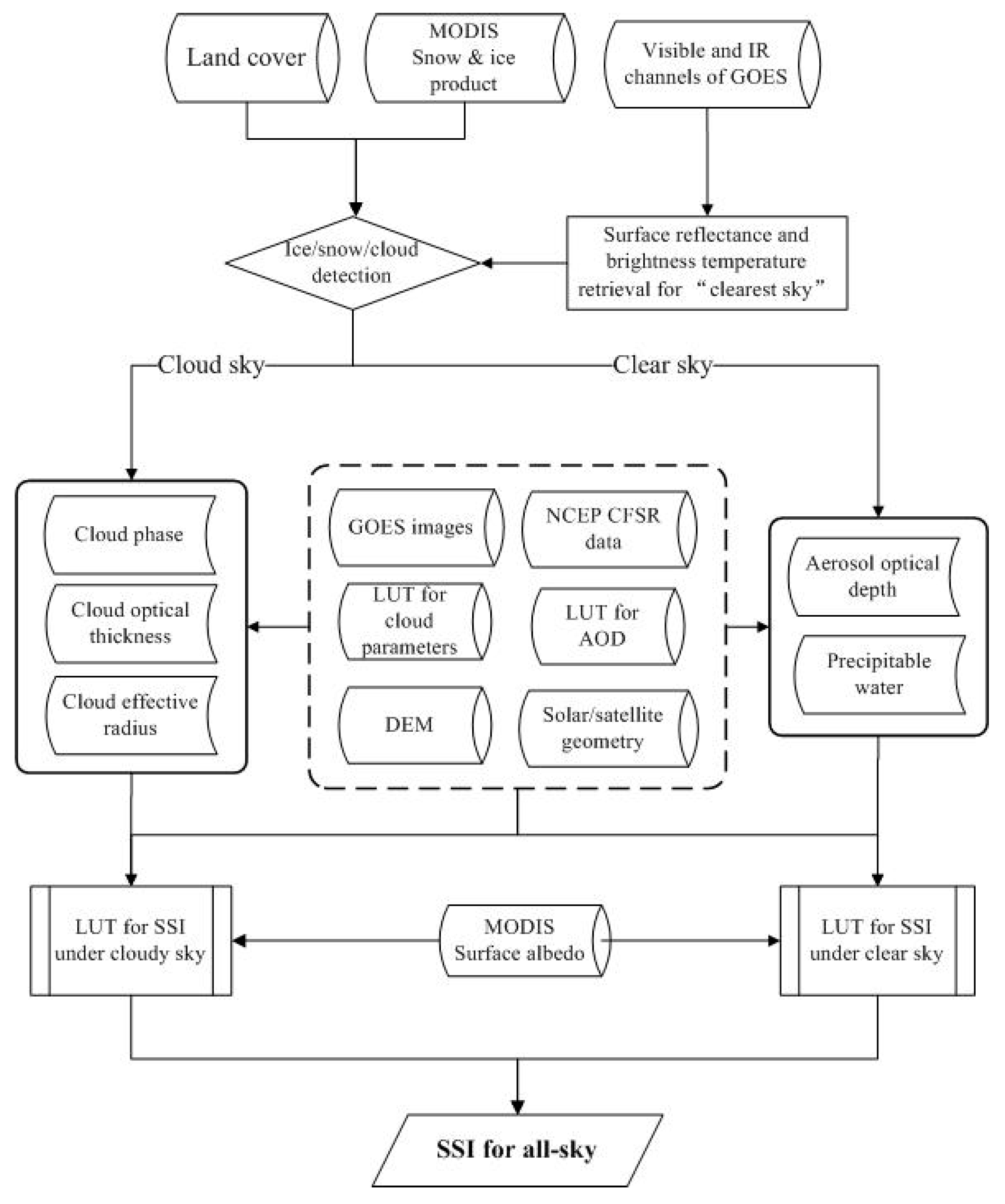
2.2.4. All-Sky SSI Estimation
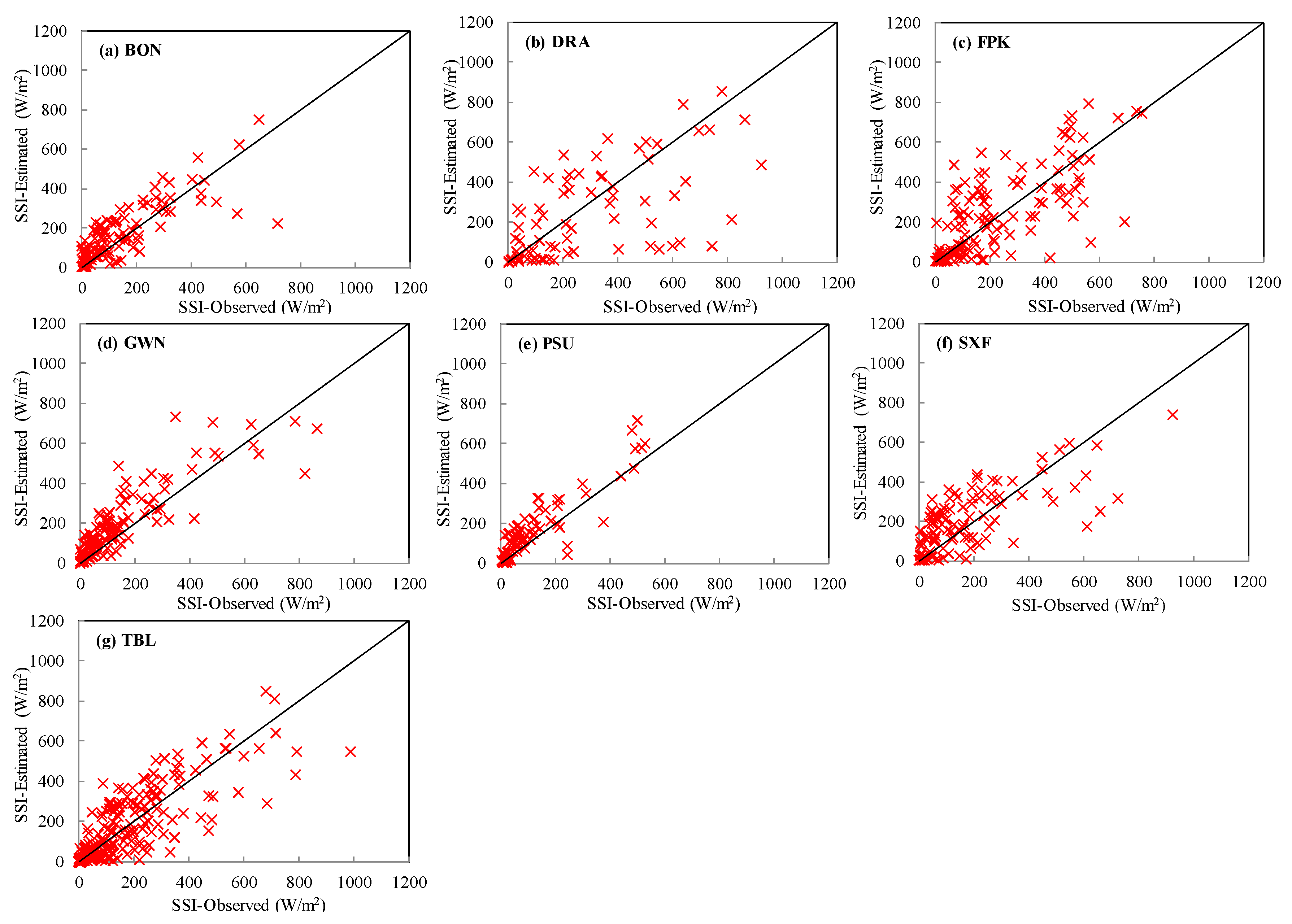
3. Results
4. Discussion
4.1. Comparison with Other SSI Estimates
4.2. Error Analysis in SSI Retrieval
5. Conclusions
Acknowledgments
Author Contributions
Conflicts of Interest
References
- Wild, M. Global dimming and brightening: A review. J. Geophys. Res. Atmos. 2009, 114. [Google Scholar] [CrossRef]
- Houborg, R.; Soegaard, H.; Emmerich, W.; Moran, S. Inferences of all-sky solar irradiance using Terra and Aqua MODIS satellite data. Int. J. Remote Sens. 2007, 28, 4509–4535. [Google Scholar] [CrossRef]
- Huang, J.; Yu, H.; Guan, X.; Wang, G.; Guo, R. Accelerated dryland expansion under climate change. Nat. Clim. Chang. 2016, 6, 166–171. [Google Scholar] [CrossRef]
- Zhang, X.; Liang, S.; Zhou, G.; Wu, H.; Zhao, X. Generating Global LAnd Surface Satellite incident shortwave radiation and photosynthetically active radiation products from multiple satellite data. Remote Sens. Environ. 2014, 152, 318–332. [Google Scholar] [CrossRef]
- Trenberth, K.E. An imperative for climate change planning: Tracking Earth’s global energy. Curr. Opin. Environ. Sustain. 2009, 1, 19–27. [Google Scholar] [CrossRef]
- Alexandri, G.; Georgoulias, A.K.; Meleti, C.; Balis, D.; Kourtidis, K.A.; Sanchez-Lorenzo, A.; Trentmann, J.; Zanis, P. A high resolution satellite view of surface solar radiation over the climatically sensitive region of Eastern Mediterranean. Atmos. Res. 2017, 188, 107–121. [Google Scholar] [CrossRef]
- Yang, K.; Koike, T.; Ye, B. Improving estimation of hourly, daily, and monthly solar radiation by importing global data sets. Agric. For. Meteorol. 2006, 137, 43–55. [Google Scholar] [CrossRef]
- Wang, L.; Kisi, O.; Zounemat-kermani, M.; Ariel, G.; Zhu, Z.; Gong, W. Solar radiation prediction using different techniques : Model evaluation and comparison. Renew. Sustain. Energy Rev. 2016, 61, 384–397. [Google Scholar] [CrossRef]
- Shamim, M.A.; Remesan, R.; Bray, M.; Han, D. An improved technique for global solar radiation estimation using numerical weather prediction. J. Atmos. Sol. Terr. Phys. 2015, 129, 13–22. [Google Scholar] [CrossRef]
- Zou, L.; Wang, L.; Lin, A.; Zhu, H.; Peng, Y.; Zhao, Z. Estimation of global solar radiation using an arti fi cial neural network based on an interpolation technique in southeast China. J. Atmos. Sol. Terr. Phys. 2016, 146, 110–122. [Google Scholar] [CrossRef]
- Xie, Y.; Sengupta, M.; Dudhia, J. A Fast All-sky Radiation Model for Solar applications (FARMS): Algorithm and performance evaluation. Sol. Energy 2016, 135, 435–445. [Google Scholar] [CrossRef]
- Zou, L.; Wang, L.; Xia, L.; Lin, A.; Hu, B.; Zhu, H. Prediction and comparison of solar radiation using improved empirical models and Adaptive Neuro-Fuzzy Inference Systems. Renew. Energy 2017, 106, 343–353. [Google Scholar] [CrossRef]
- Yeom, J.; Seo, Y.; Kim, D.; Han, K. Solar Radiation Received by Slopes Using COMS Imagery, a Physically Based Radiation Model, and GLOBE. J. Sens. 2016, 2016, 4834579. [Google Scholar] [CrossRef]
- Tang, W.; Qin, J.; Yang, K.; Liu, S.; Lu, N.; Niu, X. Retrieving high-resolution surface solar radiation with cloud parameters derived by combining MODIS and MTSAT data. Atmos. Chem. Phys. 2016, 16, 2543–2557. [Google Scholar] [CrossRef]
- Arbizu-Barrena, C.; Ruiz-Arias, J.A.; Rodríguez-Benítez, F.J.; Pozo-Vázquez, D.; Tovar-Pescador, J. Short-term solar radiation forecasting by advecting and diffusing MSG cloud index. Sol. Energy 2017, 155, 1092–1103. [Google Scholar] [CrossRef]
- Perez, R.; Seals, R.; Zelenka, A. Comparing satellite remote sensing and ground network measurements for the production of site/time specific irradiance data. Sol. Energy 1997, 60, 89–96. [Google Scholar] [CrossRef]
- Bishop, J.K.B.; Rossow, W.B. Spatial and Temporal Variability of Global Surface Solar Irradiance. J. Geophys. Res. 1991, 96, 16839–16858. [Google Scholar] [CrossRef]
- Li, Z.; Leighton, H. Global climatologies of solar radiation budgets at the surface and in the atmosphere from 5 years of ERBE data. J. Geophys. Res. Atmos. 1993, 98, 4919–4930. [Google Scholar] [CrossRef]
- Kalnay, E.; Kanamitsu, M.; Kistler, R.; Collins, W.; Deaven, D.; Gandin, L.; Iredell, M.; Saha, S.; White, G.; Woollen, J.; et al. The NCEP/NCAR 40-Year Reanalysis Project. Bull. Am. Meteorol. Soc. 1996, 77, 437–471. [Google Scholar] [CrossRef]
- Kato, S.; Loeb, N.G.; Rose, F.G.; Doelling, D.R.; Rutan, D.A.; Caldwell, T.E.; Yu, L.; Weller, R.A. Surface Irradiances Consistent with CERES-Derived Top-of-Atmosphere Shortwave and Longwave Irradiances. J. Clim. 2012, 26, 2719–2740. [Google Scholar] [CrossRef]
- Müller, R.; Pfeifroth, U.; Träger-Chatterjee, C.; Trentmann, J.; Cremer, R. Digging the METEOSAT treasure-3 decades of solar surface radiation. Remote Sens. 2015, 7, 8067–8101. [Google Scholar] [CrossRef]
- Liang, S.; Zhao, X.; Liu, S.; Yuan, W.; Cheng, X.; Xiao, Z.; Zhang, X.; Liu, Q.; Cheng, J.; Tang, H.; et al. A long-term Global LAnd Surface Satellite (GLASS) data-set for environmental studies. Int. J. Digit. Earth 2013, 6, 5–33. [Google Scholar] [CrossRef]
- Zhang, X.; Liang, S.; Wild, M.; Jiang, B. Analysis of surface incident shortwave radiation from four satellite products. Remote Sens. Environ. 2015, 165, 186–202. [Google Scholar] [CrossRef]
- Seager, R.; Blumenthal, M.B. Modeling Tropical Pacific Sea Surface Temperature with Satellite-Derived Solar Radiative Forcing. J. Clim. 1994, 7, 1943–1957. [Google Scholar] [CrossRef]
- Pinker, R.T.; Laszlo, I. Effects of Spatial Sampling of Satellite Data on Derived Surface Solar Irradiance. J. Atmos. Ocean. Technol. 1991, 8, 96–107. [Google Scholar] [CrossRef]
- Mathiesen, P.; Kleissl, J. Evaluation of numerical weather prediction for intra-day solar forecasting in the continental United States. Sol. Energy 2011, 85, 967–977. [Google Scholar] [CrossRef]
- Lara-Fanego, V.; Ruiz-Arias, J.A.; Pozo-Vázquez, D.; Santos-Alamillos, F.J.; Tovar-Pescador, J. Evaluation of the WRF model solar irradiance forecasts in Andalusia (southern Spain). Sol. Energy 2012, 86, 2200–2217. [Google Scholar] [CrossRef]
- Liang, S.; Zheng, T.; Liu, R.; Fang, H.; Tsay, S.-C.; Running, S. Estimation of incident photosynthetically active radiation from Moderate Resolution Imaging Spectrometer data. J. Geophys. Res. 2006, 111, D15208. [Google Scholar] [CrossRef]
- Qin, J.; Tang, W.; Yang, K.; Lu, N.; Niu, X.; Liang, S. An efficient physically based parameterization to derive surface solar irradiance based on satellite atmospheric products. J. Geophys. Res. Atmos. 2015, 120, 4975–4988. [Google Scholar] [CrossRef]
- Sun, Z.; Liu, A. Fast scheme for estimation of instantaneous direct solar irradiance at the earth’s surface. Sol. Energy 2013, 98, 125–137. [Google Scholar] [CrossRef]
- Alexandri, G.; Georgoulias, A.K.; Zanis, P.; Katragkou, E.; Tsikerdekis, A.; Kourtidis, K.; Meleti, C. On the ability of RegCM4 regional climate model to simulate surface solar radiation patterns over Europe: An assessment using satellite-based observations. Atmos. Chem. Phys. 2015, 15, 13195–13216. [Google Scholar] [CrossRef]
- Chen, M.; Zhuang, Q.; He, Y. An efficient method of estimating downward solar radiation based on the MODIS observations for the use of land surface modeling. Remote Sens. 2014, 6, 7136–7157. [Google Scholar] [CrossRef]
- Barzin, R.; Shirvani, A.; Lotfi, H. Estimation of daily average downward shortwave radiation from MODIS data using principal components regression method: Fars province case study. Int. Agrophys. 2017, 31, 23–34. [Google Scholar] [CrossRef]
- Cano, D.; Monget, J.; Albuisson, M.; Guillard, H.; Regas, N.; Wald, L. A method for the determination of the global solar radiation from meteorological satellite data. Sol. Energy 1986, 37, 31–39. [Google Scholar] [CrossRef]
- Castelli, M.; Stöckli, R.; Zardi, D.; Tetzlaff, A.; Wagner, J.E.; Belluardo, G.; Zebisch, M.; Petitta, M. The HelioMont method for assessing solar irradiance over complex terrain: Validation and improvements. Remote Sens. Environ. 2014, 152, 603–613. [Google Scholar] [CrossRef]
- Linares-Rodriguez, A.; Ruiz-Arias, J.A.; Pozo-Vazquez, D.; Tovar-Pescador, J. An artificial neural network ensemble model for estimating global solar radiation from Meteosat satellite images. Energy 2013, 61, 636–645. [Google Scholar] [CrossRef]
- Nakajima, T.; King, M.D.; Nakajima, T.; King, M.D. Determination of the Optical Thickness and Effective Particle Radius of Clouds from Reflected Solar Radiation Measurements. Part I: Theory. J. Atmos. Sci. 1990, 47, 1878–1893. [Google Scholar] [CrossRef]
- Platnick, S.; King, M.D.; Ackerman, S.A.; Menzel, W.P.; Baum, B.A.; Riédi, J.C.; Frey, R.A. The MODIS cloud products: Algorithms and examples from terra. IEEE Trans. Geosci. Remote Sens. 2003, 41, 459–472. [Google Scholar] [CrossRef]
- Nakajima, T.Y.; Nakajma, T. Wide-Area Determination of Cloud Microphysical Properties from NOAA AVHRR Measurements for FIRE and ASTEX Regions. J. Atmos. Sci. 1995, 52, 4043–4059. [Google Scholar] [CrossRef]
- Roebeling, R.A.; Feijt, A.J.; Stammes, P. Cloud property retrievals for climate monitoring: Implications of differences between Spinning Enhanced Visible and Infrared Imager (SEVIRI) on METEOSAT-8 and Advanced Very High Resolution Radiometer (AVHRR) on NOAA-17. J. Geophys. Res. Atmos. 2006, 111, 1–51. [Google Scholar] [CrossRef]
- Deneke, H.M.; Feijt, A.J.; Roebeling, R.A. Estimating surface solar irradiance from METEOSAT SEVIRI-derived cloud properties. Remote Sens. Environ. 2008, 112, 3131–3141. [Google Scholar] [CrossRef]
- Saha, S.; Moorthi, S.; Wu, X.; Wang, J.; Nadiga, S.; Tripp, P.; Behringer, D.; Hou, Y.T.; Chuang, H.Y.; Iredell, M.; et al. The NCEP climate forecast system version 2. J. Clim. 2014, 27, 2185–2208. [Google Scholar] [CrossRef]
- Augustine, J.A.; DeLuisi, J.J.; Long, C.N. SURFRAD—A National Surface Radiation Budget Network for Atmospheric Research. Bull. Am. Meteorol. Soc. 2000, 81, 2341–2357. [Google Scholar] [CrossRef]
- Ricchiazzi, P.; Yang, S.; Gautier, C.; Sowle, D. SBDART: A Research and Teaching Software Tool for Plane-Parallel Radiative Transfer in the Earth’s Atmosphere. Bull. Am. Meteorol. Soc. 1998, 79, 2101–2114. [Google Scholar] [CrossRef]
- Popp, C.; Hauser, A.; Foppa, N.; Wunderle, S. Remote sensing of aerosol optical depth over central Europe from MSG-SEVIRI data and accuracy assessment with ground-based AERONET measurements. J. Geophys. Res. Atmos. 2007, 112, 1–16. [Google Scholar] [CrossRef]
- D’Entremont, R.P.; Gustafson, G.B. Analysis of Geostationary Satellite Imagery Using a Temporal-Differencing Technique. Earth Interact. 2003, 7, 1–25. [Google Scholar] [CrossRef]
- Choi, Y.S.; Ho, C.H.; Ahn, M.H.; Kim, Y.M. An exploratory study of cloud remote sensing capabilities of the Communication, Ocean and Meteorological Satellite (COMS) imagery. Int. J. Remote Sens. 2007, 28, 4715–4732. [Google Scholar] [CrossRef]
- Huang, G.; Li, X.; Huang, C.; Liu, S.; Ma, Y.; Chen, H. Representativeness errors of point-scale ground-based solar radiation measurements in the validation of remote sensing products. Remote Sens. Environ. 2016, 181, 198–206. [Google Scholar] [CrossRef]
- Ryu, Y.; Jiang, C.; Kobayashi, H.; Detto, M. MODIS-derived global land products of shortwave radiation and diffuse and total photosynthetically active radiation at 5 km resolution from 2000. Remote Sens. Environ. 2018, 204, 812–825. [Google Scholar] [CrossRef]


| Input Variable | Value Range | Increment |
|---|---|---|
| Solar zenith angle | 0–89° | 5° |
| Viewing zenith angle | 0–89° | 5° |
| Relative azimuth angle | 0–180° | 30° |
| Aerosol horizontal visibility | 5, 10, 20, 30, 40, 50, 70, 100 km | - |
| Aerosol type | Rural | - |
| Water vapor | 0.01–5.0 g/cm2 | 0.5 |
| Surface altitude | 0–6 km | 1 km |
| Surface reflectance | 0–1.0 | 0.1 |
| Input Variable | Value Range | Increment |
|---|---|---|
| Solar zenith angle | 0–89° | 5° |
| Viewing zenith angle | 0–89° | 5° |
| Relative azimuth angle | 0–180° | 30° |
| COT | 0.5, 1, 2, 5, 8, 11, 15, 20, 30, 50, 70, 100 | - |
| ER (μm) | Water cloud: 2, 4, 8, 16, 32 Ice cloud: 2, 4, 8, 16, 32, 64 | - |
| Surface albedo | 0–1.0 | 0.1 |
| Surface temperature (K) | 280–320 | 2 |
| Cloud-top temperature | 195–300 | 5 |
| Cloud phase | Water, ice | - |
| Site | Latitude | Longitude | Clear Sky | Cloudy Sky | All Sky | ||||||
|---|---|---|---|---|---|---|---|---|---|---|---|
| R2 | BIAS W/m2 (%) | RMSE W/m2 (%) | R2 | BIAS W/m2 (%) | RMSE W/m2 (%) | R2 | BIAS W/m2 (%) | RMSE W/m2 (%) | |||
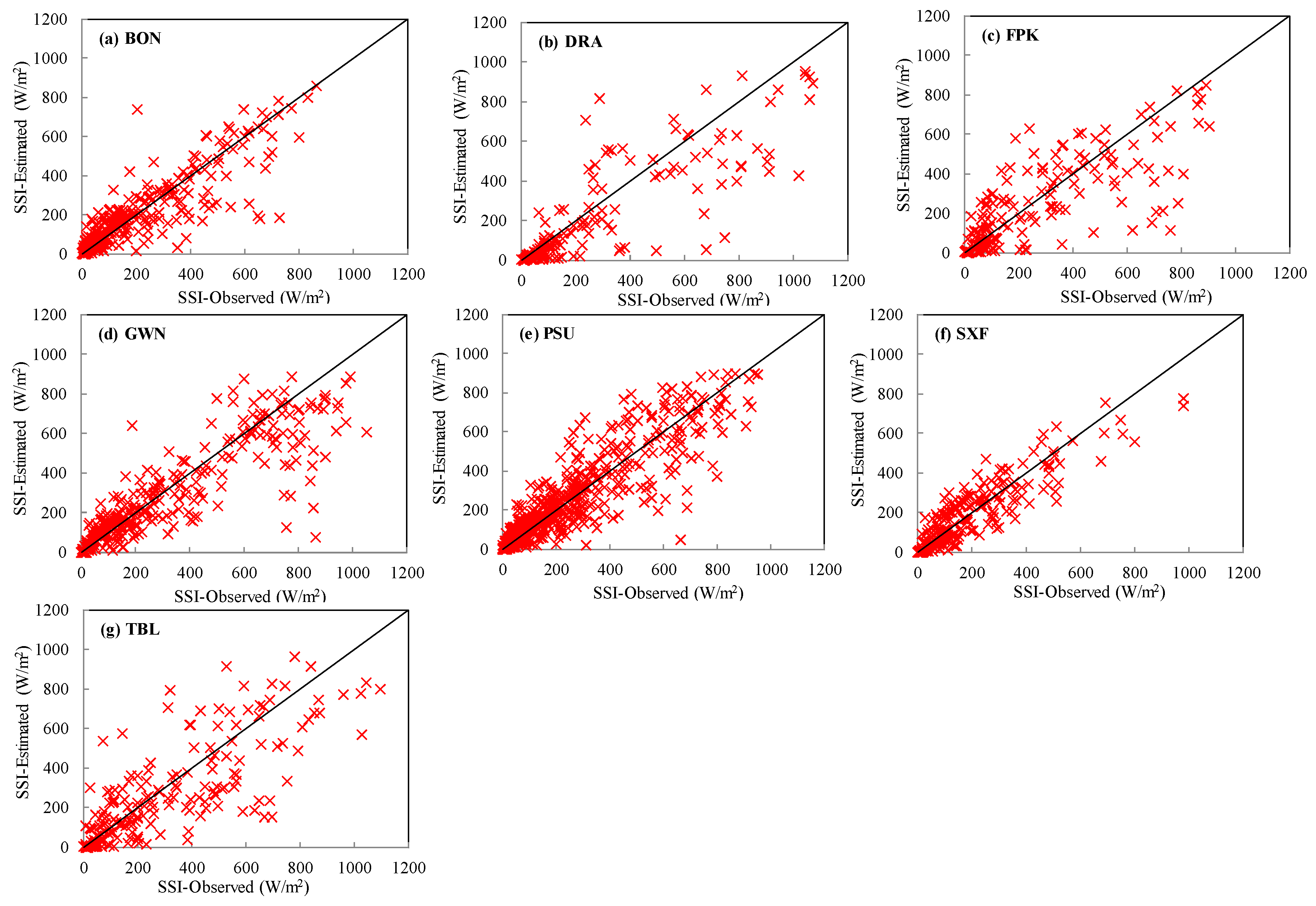
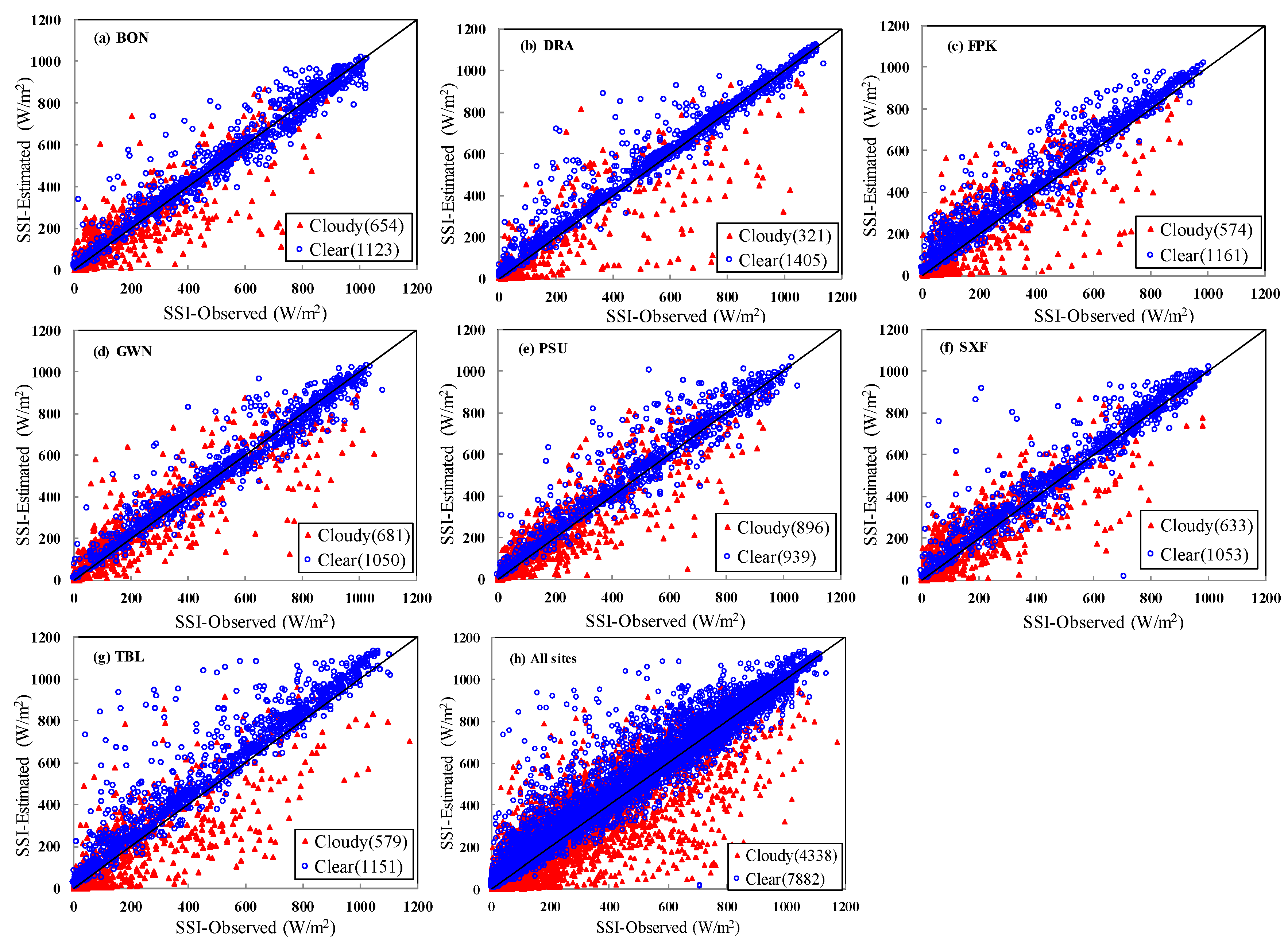
| BON | 40.06°N | 88.37°W | 0.96 | 6.4 (1.3) | 61.0 (12.6) | 0.72 | 4.97 (2.4) | 111.4 (53.6) | 0.92 | 4.5 (1.2) | 83.3 (21.7) |
| DRA | 36.63°N | 116.02°W | 0.97 | 19.0 (3.6) | 61.4 (11.8) | 0.63 | −54.5 (−18.6) | 178.2 (60.9) | 0.92 | 5.3 (1.1) | 94.8 (19.8) |
| FPK | 48.31°N | 105.10°W | 0.94 | 43.8 (10.9) | 79.9 (19.9) | 0.60 | −0.1 (−0.04) | 141.5 (65.2) | 0.87 | 29.3 (8.6) | 104.4 (30.7) |
| GWN | 34.25°N | 89.87°W | 0.96 | 2.1 (0.4) | 62.2 (12.1) | 0.76 | −2.2 (−0.9) | 122.3 (47.9) | 0.91 | 0.4 (0.1) | 90.7 (22.1) |
| PSU | 40.72°N | 77.93°W | 0.93 | 25.7 (5.7) | 81.5 (18.2) | 0.80 | 6.0 (2.8) | 98.5 (45.2) | 0.90 | 16.1 (4.8) | 90.2 (26.9) |
| SXF | 43.73°N | 96.62°W | 0.92 | 20.6 (4.3) | 81.5 (17.1) | 0.69 | 5.7 (2.7) | 111.5 (53.8) | 0.90 | 15.0 (4.0) | 93.9 (25.1) |
| TBL | 48.31°N | 105.24°W | 0.90 | 65.2 (13.6) | 118.6 (24.7) | 0.60 | −28.7 (−11.1) | 155.6 (60.0) | 0.84 | 33.8 (8.3) | 132.1 (32.5) |
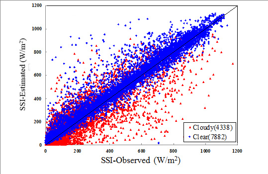
| All | 0.94 | 26.4 (5.5) | 80.0 (16.8) | 0.69 | −5.9 (−2.6) | 127.6 (55.1) | 0.89 | 14.9 (3.8) | 99.5 (25.5) | ||
| Site | R2 | BIAS (W/m2) | RMSE (W/m2) |
|---|---|---|---|
| BON | 0.86 | 20 | 100 |
| DRA | 0.88 | −55 | 119 |
| FPK | 0.82 | 5.5 | 111 |
| GWN | 0.92 | 1.7 | 86 |
| PSU | 0.87 | 12 | 100 |
| SXF | 0.86 | 14 | 102 |
| TBL | 0.77 | −8.7 | 140 |
| Site | Clear Sky (W/m2) | All Sky (W/m2) | ||||||
|---|---|---|---|---|---|---|---|---|
| Terra | Aqua | Terra | Aqua | |||||
| BIAS | RMSE | BIAS | RMSE | BIAS | RMSE | BIAS | RMSE | |
| BON | 11.5 | 41.1 | 15.3 | 54.4 | 4.0 | 86.3 | 7.6 | 95.0 |
| DRA | −11.3 | 41.9 | 8.4 | 34.4 | −11.0 | 55.0 | 8.1 | 69.7 |
| FPK | 20.2 | 43.8 | 29.9 | 49.0 | −4.3 | 105.6 | 7.8 | 95.1 |
| GWN | 21.7 | 47.2 | 24.7 | 56.7 | 17.1 | 72.4 | 22.0 | 92.8 |
| PSU | 27.0 | 57.8 | 25.1 | 59.7 | 21.8 | 101.7 | 15.1 | 99.0 |
| SXF | 17.7 | 43.3 | 19.1 | 47.0 | −5.3 | 101.0 | −2.2 | 98.8 |
| TBL | 2.1 | 37.6 | 7.1 | 42.9 | −17.7 | 113.6 | −1.9 | 123.0 |
| Site | Water Clouds | Ice Clouds | Mixed Clouds | Undetected Clouds | ||||||
|---|---|---|---|---|---|---|---|---|---|---|
| R2 | Bias W/m2 (%) | RMSE W/m2 (%) | NO. | R2 | Bias W/m2 (%) | RMSE W/m2 (%) | NO. | NO. | NO. | |
| BON | 0.74 | −8 (−3.5) | 106 (49.5) | 280 | 0.66 | 27 (19.8) | 93 (68.7) | 121 | 222 | 31 |
| DRA | 0.70 | −63 (−21.0) | 178 (59.6) | 149 | 0.38 | −44 (−15.7) | 211 (75.3) | 78 | 74 | 20 |
| FPK | 0.62 | −25 (−10.0) | 157 (63.7) | 187 | 0.54 | 15 (6.6%) | 150 (67.2) | 133 | 220 | 34 |
| GWN | 0.78 | −31 (−10.6) | 136 (46.3) | 326 | 0.75 | 45 (32.0) | 101 (71.2) | 130 | 181 | 44 |
| PSU | 0.81 | −1 (−0.42) | 105 (43.7) | 576 | 0.81 | 44 (35.8) | 83 (67.7) | 83 | 217 | 20 |
| SXF | 0.80 | −5 (−2.6) | 80 (43.0) | 233 | 0.49 | 29 (16.5) | 135 (78.1) | 109 | 243 | 47 |
| TBL | 0.64 | −38 (−12.9) | 169 (57.5) | 197 | 0.61 | −0.2 (−0.1) | 118 (61.1) | 186 | 173 | 20 |
© 2018 by the authors. Licensee MDPI, Basel, Switzerland. This article is an open access article distributed under the terms and conditions of the Creative Commons Attribution (CC BY) license (http://creativecommons.org/licenses/by/4.0/).
Share and Cite
Zhang, H.; Huang, C.; Yu, S.; Li, L.; Xin, X.; Liu, Q. A Lookup-Table-Based Approach to Estimating Surface Solar Irradiance from Geostationary and Polar-Orbiting Satellite Data. Remote Sens. 2018, 10, 411. https://doi.org/10.3390/rs10030411
Zhang H, Huang C, Yu S, Li L, Xin X, Liu Q. A Lookup-Table-Based Approach to Estimating Surface Solar Irradiance from Geostationary and Polar-Orbiting Satellite Data. Remote Sensing. 2018; 10(3):411. https://doi.org/10.3390/rs10030411
Chicago/Turabian StyleZhang, Hailong, Chong Huang, Shanshan Yu, Li Li, Xiaozhou Xin, and Qinhuo Liu. 2018. "A Lookup-Table-Based Approach to Estimating Surface Solar Irradiance from Geostationary and Polar-Orbiting Satellite Data" Remote Sensing 10, no. 3: 411. https://doi.org/10.3390/rs10030411